Water sources effects on soil salinity and biomass production of agriculture and agroforest systems in raised fields

ABSTRACT

This study investigates the sources of water under four modes, namely, normal fields, Raised Fields, single agriculture in Raised Fields, and agroforest system in Raised Fields, by using a combination of δ¹⁸O, δ²H and δ¹³C and their effects on crop yield and water use efficiency. The results show that the soil electrical conductivity of Raised Fields during summer maize seasons was lower than that during winter wheat seasons, and that in the marginal regions was higher than in the central regions, because of the Water Sources. Under agroforest conditions in Raised Fields, Soil Salinity can be reduced because approximately 10% of the water originates from tree trunks. The biomass yield and intrinsic water use efficiency of winter crops under agroforest was 15.1% and 5.5% higher than that under single agriculture, respectively. Thus, soil salinization can be reduced and productivity can be increased by controlling the Water Sources in ecosystems.

KEYWORDS:

• Water salinity
• soil salinity formation
• isotope analysis
• water use efficiency

Introduction

Soil salinization has become a serious threat to global agriculture. Approximately 20% of the world’s agricultural area is affected by high soil salinity (Devkota et al. 2015; Abiala et al. 2018). Saline-alkali land is growing at an annual rate of 10%, and it is estimated that more than 50% of cultivated land will be salinized by 2050 (Jamil et al. 2011; Machado and Serralheiro 2017), and soil salinization results in significant decreases in agricultural land area, crop yield and crop quality (Shahbaz and Ashraf 2013; Elshaikh et al. 2017). The decrease in cultivated land pose major threats to the sustainable development of humankind (Shahbaz and Ashraf 2013). Thus, it is vital to control and reduce soil salinization.

Salinity is a common problem in irrigated agriculture (Sharma et al. 2014), affected by soil parent geological material, shallow and salt-rich groundwater, and salt-rich irrigation water (Nachshon 2018). Firstly, low rainfall and high evaporative demand left more salt in topsoil. Secondly, the ingress of salt water through rivers and groundwater in the coastal regions causes large-scale salinization. Moreover, the saline water is used for irrigation in some regions, which increase the salt contents in topsoil (Liu et al. 2019).

There are two ways to increase the production under soil salinity, reducing salt directly and increasing crop salt-tolerant capacities by gene-diversity (Yamaguchi and Blumwald 2005) and bio-diversity (George et al. 2012). Raised fields are a typical physical approach to reduce the salinity of saline-alkali land (Devkota et al. 2015; Velmurugan et al. 2016). Raised beds can reduce irrigation water by 25–30%, increase water use efficiency and provide better opportunities to leach salts from furrows (Bakker et al. 2010). The soil salinity in raised beds was reduced by 85% from the initial level because of the improved bed-to-furrow drainage (Velmurugan et al. 2016). However, raised beds may be prone to salt accumulation, especially under shallow water table conditions, because of the additional surface exposure and elevation (Devkota et al. 2015).

Although the salt tolerance of wheat, rice and maize are higher among cereals, those tolerance are quite lower than the plants in natural systems (Munns 2005; Shahbaz and Ashraf 2013). However, forestry is widely used on salt-affected soils because of their higher salt tolerance (Wicke et al. 2013). Agroforest systems provided an opportunity to limit salinity-related land degradation and enhance agricultural sustainability (George et al. 2012; Wicke et al. 2013), as the growth of trees can be integrated with agriculture in salt-affected soils to take advantage of ecosystem services (Singh 2017). Accordingly, the planting of native trees has been considered a restoration measure to increase biodiversity in agroforestry (Teuscher et al. 2016). Thus, can raised fields be combined with agroforestry to control saline-alkali land and increase production?

Salt and alkali ions and water in saline-alkali land often move in synergy (Liu et al. 2019). It is therefore very important to study the differences in water sources in saline-alkali land to reveal the formation mechanism of soil salinization. Stable isotopes of natural abundance can be used to determine the sources of water, carbon and nutrients and to identify the circulation of trace elements in different systems (Hopkins and Ferguson 2012), and stable isotope analysis provides a powerful and effective method for studying the distribution of water sources (Dawson et al. 2002; Jespersen et al. 2018). Soil water contains two stable isotopes of hydrogen and oxygen (δ²H and δ¹⁸O), which change with evaporation and precipitation (Jasechko et al. 2013, Rothfuss and Javaux 2017). The main possible sources of water absorbed by plants are precipitation, soil water and groundwater, which can be ascertained by analyzing and comparing the δ²H and δ¹⁸O signatures in plant tissues or xylem (Kray et al. 2012; Zhu et al. 2012). Moreover, plant roots absorb water from different water sources without evaporation. The absorption of water by roots does not lead to the isotopic differentiation of most land plants (Brunel et al. 1995; Ellsworth and Williams 2007). Therefore, the isotopic composition of water in plant tissue or xylem can be regarded as the contributions of different water sources, for example, a mixture comprising the isotopic compositions of recent rainwater, soil water and groundwater. A Bayesian mixture model contains a realistic representation of the variability of input parameters and available prior information (Parnell et al. 2013; Wang et al. 2019). In this context, the mixed subspace is composed of two tracers, δ²H and δ¹⁸O, and three possible sources: groundwater, soil water, and rainwater (Cramer et al. 1999; Zhu et al. 2012). Moreover, changes in the isotopic compositions of different tree rings are related to changes in water availability (McCarroll and Loader 2004).

The mechanisms responsible for enabling agroforest systems and raised fields to control salinization, improve crop water use and increase yield remain unclear. The hypothesis of this paper is that the differences of water sources under agriculture and agroforest systems in raised fields will affect the formation of soil salinity and crop yield. Thus, this study investigates the kinds of water sources with different salinity and the effects on soil salinity and biomass production under four modes, namely, natural ecosystems on flat land (NEF), natural ecosystems in raised fields (NER), single agriculture in raised fields (SAR), and agroforest in raised fields (FAR), to explore the optimal ecological planting mode and its theory. A combination of δ¹⁸O and δ²H signatures of groundwater, soil water and xylem branch water and δ¹³C signatures from leaves and tree cores were employed in this study.

Materials and methods

Site description

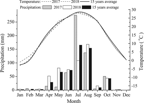
The experiment was carried out at 118° 2′ 28″ E, 37° 56′ N in Wudi County, Binzhou city, which is located on the Yellow River Delta in China from 2003 to 2018 (Figure 1). The area has a continental monsoon climate, and the average annual precipitation is 550 mm, which is mainly concentrated in summer and scarce in winter (Figure 2). The main planting mode is winter wheat-summer maize. The soil in 0–20 cm layer mainly contains sodium ions, chloride ions and acid radical ions, and the average salt content is 3.5 ‰. It also contains 8.6 g kg⁻¹ of organic matter, 0.86 g kg⁻¹ of total nitrogen, 46.2 mg kg⁻¹ of available phosphorus and 42.4 mg kg⁻¹ of available potassium; the soil pH is 7.7.

Figure 1. The experimental site.

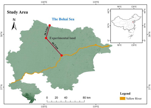
Figure 2. The distribution map of multi-year rainfall and temperature.

Experimental Design

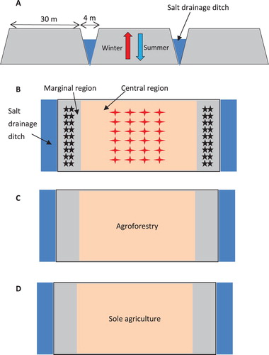
The experiment was carried out with two modes, natural ecosystem on flat land (NEF) and natural ecosystem on raised field (NER), in 2003. In 2015–2018, two other modes, single agriculture (SAR) and agroforest (FAR), were added on the raised field (Figure 3). In the SAR system, two salt discharge ditches were excavated, and a raised tract of land (planting block) 30 m wide was formed between the two ditches; either winter wheat or summer maize was planted. Similarly, in the FAR system, two salt discharge ditches were excavated, and a 30 m wide area of land was formed between the two ditches; here, winter wheat or summer maize was intercropped with forestry (black locust, Robinia pseudoacacia Linn.). The trees used in experiments were 2-year-old in 2015. Three rows of trees with 10 rows of wheat or 6 rows of maize were designed. The experimental field of each mode was 10 m long and 30 m wide and 300 m² in area. The experimental field of each mode was repeated three times. Winter wheat was sown with a seeder, the row spacing was 25 cm, and the sowing amount was 255 kg/ha. The sowing amount of summer maize was 67,500 plants/ha, and the row spacing was 45 cm. Winter wheat was sown on October 8th of every year and harvested on May 30th of the following year, whereas summer maize was sown on June 2nd of every year and harvested on October 6th of that year. Before winter wheat was sown, 100 kg ha⁻¹ of nitrogen, 60 kg ha⁻¹ of phosphorus and 75 kg ha⁻¹ of potassium were applied; before summer maize was sown, 125 kg ha⁻¹ of nitrogen, 65 kg ha⁻¹ of phosphorus and 80 kg ha⁻¹ of potassium were applied. Fertilizer was applied only to crops. No watering occurred during the whole growth period.

Figure 3. The structure and planting map of raised fields. (A) sectional drawing of a raised field (blue arrow represents summer precipitation, and red arrow represents winter groundwater), (B) vertical view (red asterisk represent sampling plots in the central regions, black asterisk represent sampling plots in the marginal regions, and number of asterisks represent the sampling numbers), (C) the intercropping of winter wheat or summer maize with forestry in the central regions, (D) either winter wheat or summer maize were planted alternately in the central regions.

Sampling method

The soil samples were collected every 45 days. Thirty sampling points were selected and divided into central and marginal regions (Figure 3(B)). Soil cores 3 cm in diameter were collected from depths of 10–30 cm, stored in a portable cooler, and cooled with liquid nitrogen. Simultaneously, the 10 crops (including leaves and stems) and 5 trees (including branches and trunks) were also immediately collected, stored in larger metallic sealed boxes, and cooled with liquid nitrogen. All samples were immediately sent to the laboratory for cryogenic distillation and analysis of δ²H, δ¹⁸O and δ¹³C. Moreover, groundwater and rainwater samples were also collected. Integrated rainfall samples were collected monthly from a rainwater collector contained a layer of mineral oil to minimize evaporation which was installed near the automated weather station in the study area according to Snyder and Williams (2000). Groundwater samples lower than 3.65 m were collected from bores in the study area using well drilling and a no-purge groundwater sampler (Rumman 2016).

At maturity, wheat within a 1 m² area or 5 m double rows of maize were harvested in each treatment with three replicates. The grains and stalks were air-dried and threshed and then weighed to calculate the biomass yield.

Water extraction and analysis

Water from the samples, including soil, crop leaves and tree trunks, was extracted by cryogenic distillation based on the methodology described in the literature (Ingraham and Shadel 1992; West et al. 2006). The extraction unit was built according to recommendations in an earlier study (Kahmen et al. 2008). The unit provides consistently high precision and accuracy for water distilled from various plant tissues and soil, especially for stable isotope analyses (Rumman 2016). Water from each sample was extracted for a minimum of 60–75 min to ensure complete extraction (West et al. 2006). After extraction, each sample was oven dried for 48 h and weighed, the result of which was then deducted from the weight of the sample measured prior to extraction to obtain the weight of the water contained within the sample. The percentage of extracted water was then calculated, and the sample was discarded and re-extracted if the percentage of extraction was <90%.

Water samples were transferred into 2 mL GC vials with a Teflon-coated rubber septum, and the transfer was conducted rapidly to avoid evaporation. The water samples were then analyzed for δ²H and δ¹⁸O using a high-temperature conversion elemental analyser coupled with an isotope ratio mass spectrometer (DELTA V Advantage, Thermo Fisher Scientific Inc.). The Vienna Standard Mean Ocean Water (VSMOW, δ¹⁸O = 0 ‰ and δ²H = 0 ‰) and Standard Light Antarctic Precipitation (SLAP, δ¹⁸O = − 55.5 ‰ and δ²H = − 427.5 ‰) references were provided by the International Atomic Energy Agency. All isotopic composition values for oxygen (δ¹⁸O) and hydrogen (δ²H) are shown in permille (‰) against the reference VSMOW or SLAP (Zhu et al. 2012; Rumman 2016).

¹³C Isotope analysis of wood cores

Five similar size trees were selected for wood core sampling in 2018, and wood cores were collected from Robinia pseudoacacia, which was available in the FAR system. The outer surface of each wood core was polished with sandpaper (Brookhouse 2006); then, the wood cores were sliced at each 0.5 cm interval with a microtome to obtain heartwood samples. Each slice was completely dried in an oven at 60°C for five days and then finely and homogeneously ground, after which 1–2 mg of ground material was taken and loaded into 5 mm × 5 mm tin capsules for δ¹³C analysis, which yielded three representative independent values per tree. δ¹³C vs Pee Dee Belemnite (PDB) was measured using a mass spectrometer (DELTA V Advantage Thermo Fisher Scientific Inc.). Atropine and acetanilide were used as laboratory standard references, and the results were normalized with the international standards Sucrose (IAEA-CH-6, δ¹³C vs PDB = −10.45 ‰), Cellulose (IAEA-CH-3, δ¹³C vs PDB = −24.72 ‰) and Graphite (USGS24, δ¹³C vs PDB = −16.05 ‰) (Rumman 2016).

Data analysis

The electrical conductivity of the saturation extract (ECse mS cm⁻¹ 25°C) was determined to measure the soil salinity (Munns 2005; Jamil et al. 2011). The water use efficiency was calculated for crop leaves. The stable carbon isotope in each plant was used to obtain the intrinsic water use efficiency (iWUE, mmol CO₂ mol⁻¹ H₂O) using the equations given by McCarroll and Loader (2004) as follows: (1) $\text{iWUE}=\frac{A}{g}=C_a\left[1-\left(\frac{C_i}{C_a}\right)\right]\cdot \left(0.625\right)$(1) (2) $\frac{C_i}{C_a}=\frac{\left({\delta }^{13}{C}_{\mathrm{p}\mathrm{l}\mathrm{a}\mathrm{n}\mathrm{t}}-{\delta }^{13}{C}_{\mathrm{a}\mathrm{i}\mathrm{r}}+a\right)}{\left(b-a\right)}$(2) where a is the discrimination (−4.4 ‰) against ¹³CO₂ during diffusion through the stomata, b is the net discrimination (−27 ‰) due to carboxylation (Farquhar et al. 1982), and c_i and c_a are the concentrations of intercellular and ambient CO₂, respectively (Leavitt et al. 2003). A is the rate of CO₂ assimilation, and g is the stomatal conductance. ¹³ C_plant and ¹³ C_air are the C isotopes of the plant sample and air, respectively (Busaria et al. 2016).

The stable isotope analysis tool in the R package siar was used to estimate proportional source contributions (Parnell et al. 2010; Wang et al. 2019). The siar tool uses a Bayesian approach based on the Gaussian likelihood to fit probability models to isotopic data and estimates the most likely proportion of water taken up from each source in plant water (Parnell et al. 2010). The siar package allows the incorporation of variability and uncertainty between sources in the model, as well as any number of sources (Hopkins and Ferguson 2012). Additionally, groundwater, irrigation and rainwater were considered potential sources of water uptake in the model. The isotopic signature and standard error of each potential source were used as the inputs for the model, and the plant/soil water isotopic signals were used as the ‘target’ values (Parnell et al. 2010). The trophic enrichment factor (TEF) of the model was set to 0 because no enrichment of isotopes occurs during the uptake of water from soil by roots (Ehleringer and Dawson T 1992). The concentration dependence was also set to 0. Furthermore, the siar package uses the basic methodology, so a linear mixing model could be used to calculate the respective contributions of sources (Phillips and Gregg 2003). Equations (3)–(5) were simplified for the three sources to calculate the proportions (p_A, p_B, and p_c) of the possible ѕourceѕ (δ_A, δ_B, and δ_C), which resulted in a mixture of isotopes (δ_M). δX_M and δY_M represent the δ²Н and δ¹⁸O values, respectively, in crop leaves or soil water. p_X (%) represents the fractional contribution of δ²Н and δ¹⁸O of each possible water source (A–C), such as precipitation (including irrigation water), glaciers and groundwater. Calculating the source of water by using two isotopes is more accurate than using only one isotope (Snyder and Williams 2000; Zhang et al. 2009). (3) $\delta X_M=P_A\delta X_A+P_B\delta X_B+P_C\delta X_C$(3) (4) $\delta Y_M=P_A\delta Y_A+P_B\delta Y_B+P_C\delta Y_C$(4) (5) $1=P_A+P_B+P_C$(5)

Analysis of variance (ANOVA) was conducted by using SPSS 19.0 software (SPSS Inc., Chicago, IL, USA), while least significance difference (LSD, P < 0.05) analysis was used for the mean significance test (Hu et al. 2013; Guo et al. 2016), and figures were generated using Sigma-Plot 11.0 (Systat Software Inc., Chicago, IL, USA) and Origin 8.5 (Origin Lab corporation, Northampton, USA).

Results

Variations in soil electrical conductivity in raised fields over 15 years

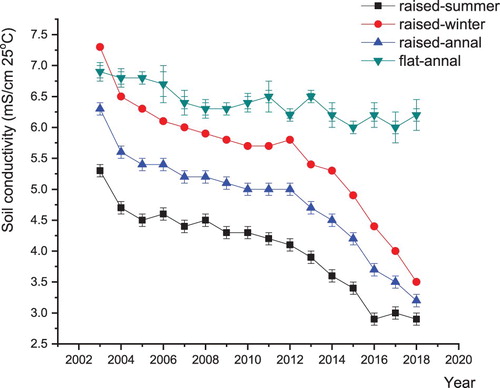
Over a period of 15 years, the electrical conductivity of 0-20 cm soil layers was significantly reduced by using a raised field (Figure 4). The soil electrical conductivity in 2018 was an average of 49.2% lower than that in 2003. Moreover, the average soil electrical conductivity during winter wheat seasons was 37.2% higher than that during summer maize seasons, and it reached a very significant level. However, there was no significant difference in the soil electrical conductivity among the different years for flat land.

Figure 4. The variations in soil electrical conductivity at depths of 0–30 cm in normal fields and raised fields. The soil electrical conductivity is the average value from the central and marginal regions of soil. The average values, e.g. 3.0 and 4.0 mS/cm 25°C, respectively, represent 3.6 and 5 ‰ NaCl contents in soil at depths of 0–30 cm (soil tillage layer).

Water sources of crop leaves and rhizosphere soil in raised fields

An average of 87.8–89.6% of the water sources of crop leaves and topsoil came from groundwater during winter wheat seasons, while an average of 85.2–90.3% of the water came from Precipitation during summer maize seasons (Tables 1 and 2). The salt content of groundwater was much higher than that of rainwater. Thus, the variation in the source of water led to the difference in soil electrical conductivity between winter and summer.

Table 1. Water sources of crop leaves and crop intrinsic water use efficiency (iWUE) during winter wheat seasons in the central regions and marginal regions under single agriculture in raised fields (SAR) mode (mean ± standard deviation in brackets).

Years	Treatments	Water sources of crop leaves (%)			iWUE
		Precipitation	Groundwater	Ditch water	(mmol CO2 mol^−1 H2O)
2015	central	9.2(0.14)	89.5(0.13)	1.3(0.03)	177.6(1.01)
	marginal	4.4(0.05)	87.6(0.09)	8.0(0.13)	150.6(1.99)
2016	central	9.4(0.19)	89.7(0.08)	0.9(0.02)	179.4(1.32)
	marginal	4.1(0.09)	87.6(0.10)	8.3(0.14)	151.5(1.04)
2017	central	9.1(0.11)	89.3(0.14)	1.6(0.03)	178.5(1.21)
	marginal	3.8(0.04)	87.8(0.15)	8.4(0.15)	150.1(0.98)
2018	central	9.9(0.09)	89.8(0.07)	0.3(0.01)	177.4(1.13)
	marginal	4.5(0.08)	88.2(0.10)	7.3(0.05)	153.1(1.26)
Average	central	9.4(0.13)	89.6(0.11)	1.0(0.02)	178.2(1.17)
	marginal	4.2(0.07)	87.8(0.11)	8.0(0.12)	151.3(1.32)

Table 2. Water sources of crop leaves and crop intrinsic water use efficiency (iWUE) during summer maize seasons in the central regions and marginal regions under single agriculture in raised fields (SAR) mode (mean ± standard deviation in brackets).

Years	Treatments	Water sources of crop leaves (%)			iWUE
		Precipitation	Groundwater	Ditch water	(mmol CO2 mol^−1 H2O)
2015	central	90.3(0.12)	8.8(0.08)	0.9(0.01)	222.4(1.16)
	marginal	84.9(0.09)	9.4(0.04)	5.7(0.02)	210.2(1.07)
2016	central	90.1(0.11)	8.7(0.04)	1.2(0.03)	220.1(1.20)
	marginal	85.1(0.13)	9.3(0.07)	5.6(0.02)	208.6(0.97)
2017	central	90.2(0.11)	8.9(0.05)	0.9(0.02)	220.9(0.89)
	marginal	85.3(0.11)	9.3(0.04)	5.4(0.02)	209.4(1.03)
2018	central	90.5(0.13)	9.0(0.04)	0.5(0.01)	223.2(0.99)
	marginal	85.5(0.11)	9.4(0.02)	5.1(0.02)	210.6(1.12)
Average	central	90.2(0.12)	8.9(0.05)	0.9(0.02)	221.7(1.06)
	marginal	85.1(0.11)	9.4(0.04)	5.5(0.02)	209.7(1.05)

As another interesting phenomenon, the soil electrical conductivity in the marginal regions was significantly higher than that in the central regions (Tables 3 and 4). During winter wheat seasons, the soil electrical conductivity in the marginal regions was 28.9% higher than that in the central regions; however, during summer maize seasons, the soil electrical conductivity in the marginal regions was 11.8% higher than that in the central regions. This may be because in the central regions during winter, on average, 8.9%, 1.0% and 90.1% of the water absorbed by crops and topsoil originated from precipitation, salt drainage ditches and groundwater, respectively, showing that the water from precipitation was significantly greater than that from salt drainage ditches. However, in the marginal regions, on average, 3.7%, 8.4% and 87.8% of the water in the crops and rhizosphere soil originated from precipitation, salt drainage ditches and groundwater, respectively; in this case, the amount of water from salt drainage ditches was significantly larger than that from precipitation. This reversal caused the difference in soil electrical conductivity between the central regions and marginal regions during winter wheat seasons. Furthermore, the average iWUE of the crops in the central regions was 17.8% higher than that of the crops in the marginal regions (Table 1).

Table 3. Water sources of topsoil and soil electrical conductivity of the saturation extract (EC_se) during winter wheat seasons in the central regions and marginal regions under single agriculture in raised fields (SAR) mode (mean ± standard deviation in brackets).

Years	Treatments	Water sources of topsoil (%)			Soil ECse
		Precipitation	Groundwater	Ditch water	(mS/cm 25°C)
2015	central	8.3(0.11)	90.7(0.10)	1.0(0.02)	3.1(0.04)
	marginal	3.2(0.05)	87.5(0.12)	9.3(0.12)	3.9(0.02)
2016	central	8.8(0.13)	90.9(0.11)	0.3(0.01)	3.3(0.01)
	marginal	3.6(0.03)	88.2(0.15)	8.2(0.09)	4.0(0.02)
2017	central	8.2(0.08)	90.2(0.16)	1.6(0.04)	3.2(0.01)
	marginal	3.3(0.03)	87.6(0.09)	9.1(0.17)	4.1(0.02)
2018	central	8.3(0.12)	90.4(0.11)	1.3(0.02)	2.9(0.04)
	marginal	2.9(0.03)	88.1(0.12)	9.0(0.06)	4.1(0.04)
Average	central	8.4(0.11)	90.5(0.12)	1.1(0.02)	3.1(0.03)
	marginal	3.3(0.04)	87.8(0.12)	8.9(0.11)	4.0(0.03)

Table 4. Water sources of topsoil and soil electrical conductivity of the saturation extract (EC_se) during summer maize seasons in the central regions and marginal regions under single agriculture in raised fields (SAR) mode (mean ± standard deviation in brackets).

Years	Treatments	Water sources of topsoil (%)			Soil ECse
		Precipitation	Groundwater	Ditch water	(mS/cm 25°C)
2015	central	89.5(0.13)	9.2(0.09)	1.3(0.02)	2.8(0.02)
	marginal	83.6(0.10)	10.1(0.06)	6.3(0.02)	3.1(0.03)
2016	central	89.3(0.12)	9.5(0.05)	1.2(0.04)	2.9(0.01)
	marginal	84.0(0.12)	10.0(0.08)	6.0(0.03)	3.2(0.02)
2017	central	89.9(0.14)	9.4(0.03)	0.7(0.03)	2.7(0.03)
	marginal	83.1(0.12)	10.3(0.06)	6.6(0.01)	3.1(0.01)
2018	central	89.7(0.12)	9.7(0.02)	0.6(0.01)	2.8(0.01)
	marginal	83.4(0.12)	10.4(0.01)	6.2(0.02)	3.2(0.04)
Average	central	89.5(0.13)	9.5(0.05)	1.0(0.03)	2.8(0.02)
	marginal	83.5(0.12)	10.2(0.05)	6.3(0.02)	3.2(0.03)

Similar conclusions were obtained during summer maize seasons (Table 4). In the central regions, on average, 90%, 0.9% and 9.2% of the water in the crops and topsoil originated from precipitation, salt drainage ditches and groundwater, respectively. However, in the marginal regions, the average water sources for crops and rhizosphere soil were precipitation (84.4%), salt drainage ditches (5.9%) and groundwater (9.8%). Compared with that in the central regions, the average amount of water absorbed by the crops and rhizosphere soil in the marginal regions from salt drainage ditches increased by 556%. Because the salinity of the salt drainage ditch water and groundwater was much higher than that of the precipitation, the soil electrical conductivity in the marginal regions was 14.3% higher than that in the central regions during summer. Furthermore, the average iWUE of the crops in the central regions was 5.7% higher than that of the crops in the marginal regions (Table 2).

Biomass yield and water sources of central region crops in raised fields

The biomass yields in the SAR and FAR systems were compared in the central regions. There was no significant difference in the summer maize biomass yield between SAR and FAR (Figure 5). However, the average biomass yield of winter wheat under FAR was 15.1% higher than that under SAR from 2015 to 2018.

FIgure 5. The biomass yield of crops in the central regions from 2015 to 2018. SAR: single agriculture in raised fields, FAR: agroforest in raised fields, Biomass yield: the sum of the grains and stalks of winter wheat or summer maize.

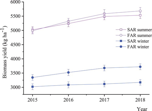
The average water sources of crop leaves under FAR were precipitation (10.6%), tree trunk water (10.3%) and groundwater (79.1%) during 2015–2018 (Table 5). In contrast, the average water sources of crop leaves under SAR were precipitation (9.2%) and groundwater (90.8%) during the same period. Thus, the proportion of groundwater was higher under SAR than under FAR. As is evident, tree trunk water can be used under FAR, which reduces the use of groundwater and consequently reduces the soil salinity. Moreover, the average crop iWUE under FAR was 5.5% higher than that under SAR during 2015–2018.

Table 5. Water sources of crop leaves and crop intrinsic water use efficiency (iWUE) during winter wheat seasons under the single agriculture in raised fields (SAR) and agroforest in raised fields (FAR) modes (mean ± standard deviation in brackets).

Years	Treatments	Water sources of crop leaves (%)			iWUE
		Precipitation	Groundwater	Tree trunk	(mmol CO2 mol^−1 H2O)
2015	SAR	9.6(0.27)	90.4(0.20)	–	176.9(2.43)
	FAR	10.8(0.56)	79.9(0.28)	9.3(0.21)	184.5(2.61)
2016	SAR	9.1(0.39)	90.9(0.18)	–	175.2(1.25)
	FAR	10.6(0.48)	79.6(0.17)	9.8(0.11)	184.2(2.14)
2017	SAR	9.0(0.21)	91.0(0.22)	–	176.5(1.42)
	FAR	10.9(0.23)	78.7(0.13)	10.4(0.16)	188.7(1.21)
2018	SAR	8.9(0.22)	91.1(0.21)	–	181.6(1.24)
	FAR	9.9(0.24)	78.6(0.22)	11.5(0.16)	192.2(2.06)
Average	SAR	9.2(0.27)	90.8(0.20)	–	177.6(1.59)
	FAR	10.6(0.38)	79.1(0.20)	10.3(0.16)	187.4(2.01)

Note: ‘–’ indicates either 0 or none.

The average water sources for the topsoil under FAR were precipitation (9.4%), tree trunk water (11.7%) and groundwater (78.9%) during 2015–2018 (Table 6). In contrast, during the same period, the average water sources for the topsoil under SAR were precipitation (8.2%) and groundwater (91.8%). Thus, the proportion of groundwater absorbed by topsoil was higher under SAR than under FAR. However, although tree trunk water can be used under FAR, thereby reducing the soil salinity, the average soil electrical conductivity under FAR was similar to that under SAR during 2015–2018.

Table 6. Water sources of topsoil and soil electrical conductivity of the saturation extract (EC_se) during winter wheat seasons under the single agriculture in raised fields (SAR) and agroforest in raised fields (FAR) modes (mean ± standard deviation in brackets).

Years	Treatments	Water sources of topsoil (%)			Soil ECse
		Precipitation	Groundwater	Tree trunk	(mS/cm 25°C)
2015	SAR	8.3(0.32)	91.7(0.27)	–	3.6(0.07)
	FAR	9.9(0.31)	78.9(0.25)	11.2(0.3)	3.5(0.08)
2016	SAR	8.0(0.31)	92.0(0.23)	–	3.1(0.04)
	FAR	9.5(0.43)	79.2(0.21)	11.3(0.13)	3.0(0.02)
2017	SAR	8.2(0.15)	91.8(0.26)	–	2.9(0.03)
	FAR	9.2(0.29)	78.8(0.17)	12.0(0.17)	3.0(0.06)
2018	SAR	8.1(0.27)	91.9(0.24)	–	2.8(0.05)
	FAR	8.9(0.16)	78.8(0.15)	12.3(0.24)	2.7(0.04)
Average	SAR	8.2(0.26)	91.8(0.25)	–	3.1(0.05)
	FAR	9.4(0.30)	78.9(0.20)	11.7(0.21)	3.0(0.05)

Note: ‘–’ indicates either 0 or none.

Δ¹³c (‰) value distribution in the heartwood of trees under agroforest conditions in raised fields

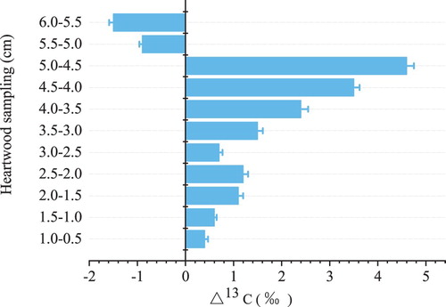
The ‘previous’ δ13C value was significantly smaller than the ‘current’ δ¹³C value in the 5.0–6.0 cm slices of heartwood (Figure 6). However, in the 0–5.0 cm slices of heartwood, the ‘previous’ δ13C value was significantly larger than the ‘current’ δ¹³C value. Thus, the δ¹³C (‰) values in the outer layer were lower than those in the inner layers, indicating that the δ¹³C (‰) values of newly formed layers in trees in raised fields are decreasing year by year.

Figure 6. The distribution of δ¹³C (‰) values in the heartwood of trees under agroforest in raised fields. The wood cores were sliced at intervals of 0.5 cm without bark from the bark side to the heartwood. For example, 1–0.5 cm represents using the ‘previous’ δ¹³C value minus the ‘current’ δ¹³C value. If the δ¹³C difference value is positive (+), it means that the ‘previous’ δ¹³C value greater than that of the ‘current.’ If the δ¹³C difference value is negative (−), it means that the ‘previous’ δ¹³C value less than that of the ‘current.’

Discussions

Raised fields have been adopted in many areas to reduce soil salinization and alleviate adverse effects on crops (Devkota et al. 2015; Velmurugan et al. 2016). The electrical conductivity of topsoil decreased significantly in the raised fields during 2003–2018. Water has a synergistic relationship with salt (Liu et al. 2019), so the movement of water can explain the changes in the salt and alkali contents in soil to a certain extent. Thus the decrease of soil electrical conductivity mainly because: (1) the increase of water use efficiency reducing the quantity of water as well as salt move to topsoil (Bakker et al. 2010); (2) a part of the soil salinity in raised beds moved downward induced by bed-to-furrow drainage (Velmurugan et al. 2016). After long-term use of raised fields, the two effects were accumulated after 15 years, which decreased the electrical conductivity of topsoil significantly.

During summer maize seasons, the main source of water for crops and topsoil came from precipitation, while during winter wheat seasons, the main source of water was groundwater. In addition, the proportion of water from salt drainage ditches in the marginal regions was larger than that in the central regions, which led to lower salt contents in the central regions than in the marginal regions. Thus, the changes of water sources led to lower soil salinity during summer maize seasons than during winter wheat seasons, and higher in the marginal regions than that in the central regions.

The soil salinity during winter wheat seasons is relatively high; therefore, winter crops are the focus of our research. In this paper, the average biomass yield of winter crops in FAR was 15.1% higher than that in SAR during 2015–2018. First, tree trunk water can be used in a FAR system, reducing the direct use of groundwater. Furthermore, trees have the ‘hydraulic lift’ functionality, which refers to the movement of water from the roots into soil layers with lower water potential (Caldwell et al. 1998). Hydraulic lift can release an average of 0.04–1.30 mm of water into the dry topsoil every day, which may supply 2–80% of transpiration water consumption (Neumann and Cardon 2012). When the topsoil is dry and competes for water uptake, the hydraulic lift induced by trees is increased, thereby absorbing more water from deep soil layers (Xi et al. 2018). Second, trees in alley agroforest systems may also conserve soil moisture and provide protection for crops (George et al. 2012). There is a relationship between the iWUE and plant water deficit (Livingston and Spittlehouse 1996 Busaria et al. 2016;). The higher iWUE of crops in FAR was attributed to the higher biomass yield during winter wheat seasons related to the better water content and lower salinity of the topsoil.

As stated earlier, the δ¹³C (‰) values of newly formed layers in trees in raised fields are decreasing year by year. Moreover, the shoot δ¹³C was affected by atmospheric pressure, temperature, and precipitation (Chen et al. 2017), and the change in the CO₂ (Ci/Ca) ratio of leaves was recorded in the cellulose of tree rings (McCarroll and Loader 2004; Máguas et al. 2011). Variable exchanges with xylem water sources during wood synthesis determine the relative strength of the source water and leaf enrichment signals (McCarroll and Loader 2004). The xylem of trees is rich in ¹³C when subjected to water stress, which reflects a reduction in stomatal conductance relative to photosynthesis. Hence, shoot and soil δ¹³C increase during drought; however, δ¹³C decreases after rewatering (Blessing et al. 2016). Such variation was more evident during spring than during summer drought (Máguas et al. 2011). Thus, the decreased δ¹³C values indicate that soil salinization is decreasing year by year.

Conclusions

The electrical conductivity of topsoil was reduced significantly by using a raised field during 2003–2018. The soil electrical conductivity during summer maize seasons was significantly lower than that during winter wheat seasons, and the soil electrical conductivity in the central regions was significantly lower than that in the marginal regions. The average biomass yield and iWUE of winter crops under FAR were 15.1% and 5.5% higher, respectively, than those under SAR during 2015–2018. The δ¹³C (‰) values of newly formed layers in trees indicated that the soil salinization is decreasing year by year by using FAR because FAR systems can use more precipitation or tree trunk water and therefore less groundwater. Thus, FAR systems could represent the optimal ecological planting mode under salt stress, as this approach can reduce soil salinization and increase both crop water use efficiency and yield by changing the water sources of soil and crops.

Acknowledgements

This work is supported by the Key Research and Development Program of Shandong (2017CXGC0308), the Funds of Shandong ‘Double Tops,’ the Shandong Province Higher Educational Science and Technology Program (J18KA132), and the State Key Laboratory of Crop Biology Priority Open Fund (2018 kf04).

HH and TN designed the study. HH, MKZ, MF, JQ, MZZ and YZ collected the samples and measured the data with support from TN. HH and TN wrote the paper with comments from MKZ, JC, YF, and GL. All authors contributed to revising the paper.

Disclosure statement

No potential conflict of interest was reported by the author(s).

Additional information

Funding

This work is supported by the Key Research and Development Program of Shandong [2017CXGC0308], the Funds of Shandong ‘Double Tops,’ the Shandong Province Higher Educational Science and Technology Program [J18KA132], and the State Key Laboratory of Crop Biology Priority Open Fund [2018 kf04].

Notes on contributors

Hengyu Hu

Hengyu Hu is a postdoctral candidate majoring in Crop science.

Mengkun Zhang

Mengkun Zhang, Min Fu and Jihao Qin are postgraduate students from Shandong Agricultural University (China), and have vast research experience in discipline of Crop Science.

Min Fu

Mengkun Zhang, Min Fu and Jihao Qin are postgraduate students from Shandong Agricultural University (China), and have vast research experience in discipline of Crop Science.

Jihao Qin

Mengkun Zhang, Min Fu and Jihao Qin are postgraduate students from Shandong Agricultural University (China), and have vast research experience in discipline of Crop Science.

Jiansheng Chen

Jiansheng Chen are working as Associate Professors in College of Agronomy, Shandong Agricultural University (China).

Yupeng Feng

Yupeng Feng is working in National Agricultural Technology Extension and Service Center, China.

Geng Li

Geng Li are working as Associate Professors in College of Agronomy, Shandong Agricultural University (China).

Mingzhen Zhai

Mingzhen Zhai and Yin Zhang are postgraduate students from Shandong Agricultural University (China), and have vast research experience in discipline of Crop Science.

Yin Zhang

Mingzhen Zhai and Yin Zhang are postgraduate students from Shandong Agricultural University (China), and have vast research experience in discipline of Crop Science.

Tangyuan Ning

Tangyuan Ning is a Professor in Crop Science. Authorship of more than 90 academic papers make it prominent in his field.

References

- Abiala MA, Abdelrahman M, Burritt DJ, Tran LSP. 2018. Salt stress tolerance mechanisms and potential applications of legumes for sustainable reclamation of salt-degraded soils. Land Degrad Dev. 29:3812–3822. doi: 10.1002/ldr.3095
- Bakker DM, Hamilton GJ, Hetherington R, Spann C. 2010. Salinity dynamics and the potential for improvement of waterlogged and saline land in a Mediterranean climate using permanent raised beds. Soil Tillage Res. 110:8–24. doi: 10.1016/j.still.2010.06.004
- Blessing CH, Barthel M, Gentsch L, Buchmann N. 2016. Strong coupling of shoot assimilation and soil respiration during drought and recovery periods in Beech as indicated by natural abundance delta(13)C measurements. Front Plant Sci. 7:1710. doi: 10.3389/fpls.2016.01710
- Brookhouse M. 2006. Eucalypt dendrochronology: past, present and potential. Aust J Bot. 54:435–449. doi: 10.1071/BT05039
- Brunel J-P, Walker GR, Kennett-Smith AK. 1995. Field validation of isotopic procedures for determining sources of water used by plants in a semi-arid environment. J Hydrol. 167:351–368. doi: 10.1016/0022-1694(94)02575-V
- Busaria MA, Salakoa FK, Tuniz C. 2016. Stable isotope technique in the evaluation of tillage and fertilizer effects on soil carbon and nitrogen sequestration and water use efficiency. Eur J Agron. 73:98–106. doi: 10.1016/j.eja.2015.11.002
- Caldwell MM, Dawson TE, Richards JH. 1998. Hydraulic lift: consequences of water efflux from the roots of plants. Oecologia. 113:151–161. doi: 10.1007/s004420050363
- Chen Z, Wang G, Jia Y. 2017. Foliar delta(13)C showed no altitudinal trend in an arid region and atmospheric pressure exerted a negative effect on plant delta(13)C. Front Plant Sci. 8:1070. doi: 10.3389/fpls.2017.01070
- Cramer VA, Thorburn PJ, Fraser GW. 1999. Transpiration and groundwater uptake from farm forest plots of Casuarina glauca and Eucalyptus camaldulensis in saline areas of southeast Queensland, Australia. Agric Water Manag. 39:187–204. doi: 10.1016/S0378-3774(98)00078-X
- Dawson TE, Mambelli S, Plamboeck AH, Templer PH, Tu KP. 2002. Stable isotopes in plant ecology. Annu Rev Ecol Syst. 33:507–559. doi: 10.1146/annurev.ecolsys.33.020602.095451
- Devkota M, Gupta RK, Martius C, Lamers JPA, Devkota KP, Sayre KD, Vlek PLG. 2015. Soil salinity management on raised beds with different furrow irrigation modes in salt-affected lands. Agric Water Manag. 152:243–250. doi: 10.1016/j.agwat.2015.01.013
- Devkota M, Martius C, Gupta RK, Devkota KP, McDonald AJ, Lamers JPA. 2015. Managing soil salinity with permanent bed planting in irrigated production systems in Central Asia. Agr Ecosyst Environ. 202:90–97. doi: 10.1016/j.agee.2014.12.006
- Ehleringer JR, Dawson T E. 1992. Water uptake by plants: perspectives from stable isotope composition. Plant Cell Environ. 15:1073–1082. doi: 10.1111/j.1365-3040.1992.tb01657.x
- Ellsworth PZ, Williams DG. 2007. Hydrogen isotope fractionation during water uptake by woody xerophytes. Plant Soil. 291:93–107. doi: 10.1007/s11104-006-9177-1
- Elshaikh NA, Zhipeng L, Dongli S, Timm LC. 2017. Increasing the okra salt threshold value with biochar amendments. J Plant Interact. 13:51–63. doi: 10.1080/17429145.2017.1418914
- Farquhar GD, O’Leary MH, Berry JA. 1982. On the relationship between carbon isotope discrimination and the intercellular carbon dioxide concentration in leaves. Aust J Plant Physiol. 9:121–137.
- George SJ, Harper RJ, Hobbs RJ, Tibbett M. 2012. A sustainable agricultural landscape for Australia: A review of interlacing carbon sequestration, biodiversity and salinity management in agroforestry systems. Agric Ecosyst Environ. 163:28–36. doi: 10.1016/j.agee.2012.06.022
- Guo L, Ning T, Nie L, Li Z, Lal R. 2016. Interaction of deep placed controlled-release urea and water retention agent on nitrogen and water use and maize yield. Eur J Agron. 75:118–129. doi: 10.1016/j.eja.2016.01.010
- Hopkins J3, Ferguson JM. 2012. Estimating the diets of animals using stable isotopes and a comprehensive Bayesian mixing model. PLoS ONE. 7:e28478. doi: 10.1371/journal.pone.0028478
- Hu H, Ning T, Li Z, Han H, Zhang Z, Qin S, Zheng Y. 2013. Coupling effects of urea types and subsoiling on nitrogen–water use and yield of different varieties of maize in northern China. Field Crops Res. 142:85–94. doi: 10.1016/j.fcr.2012.12.001
- Ingraham NL, Shadel C. 1992. A comparison of the toluene distillation and vacuum/heat methods for extracting soil water for stable isotopic analysis. J Hydrol. 140:371–387. doi: 10.1016/0022-1694(92)90249-U
- Jamil A, Riaz S, Ashraf M, Foolad MR. 2011. Gene expression profiling of plants under salt stress. Crit Rev Plant Sci. 30:435–458. doi: 10.1080/07352689.2011.605739
- Jasechko S, Sharp ZD, Gibson JJ, Birks SJ, Yi Y, Fawcett PJ. 2013. Terrestrial water fluxes dominated by transpiration. Nature. 496:347–350. doi: 10.1038/nature11983
- Jespersen RG, Leffler AJ, Oberbauer SF, Welker JM. 2018. Arctic plant ecophysiology and water source utilization in response to altered snow: isotopic (delta(18)O and delta(2)H) evidence for meltwater subsidies to deciduous shrubs. Oecologia Aug. 187:1009–1023. doi: 10.1007/s00442-018-4196-1
- Kahmen A, Simonin K, Tu KP, Merchant A, Callister A, Siegwolf R, Dawson TE, Arndt SK. 2008. Effects of environmental parameters, leaf physiological properties and leaf water relations on leaf water delta18O enrichment in different Eucalyptus species. Plant Cell Environ. Jun. 31:738–751. doi: 10.1111/j.1365-3040.2008.01784.x
- Kray JA, Cooper DJ, Sanderson JS. 2012. Groundwater use by native plants in response to changes in precipitation in an intermountain basin. J Arid Environ. 83:25–34. doi: 10.1016/j.jaridenv.2012.03.009
- Leavitt SW, Idso SB, Kimball BA, Burns JM, Sinha A, Stott L. 2003. The effect of long-term atmospheric CO2 enrichment on the intrinsic water-use efficiency of sour orange trees. Chemosphere. 50:217–222. doi: 10.1016/S0045-6535(02)00378-8
- Liu D, She D, Mu X. 2019. Water flow and salt transport in bare saline-sodic soils subjected to evaporation and intermittent irrigation with saline/distilled water. Land Degrad Dev. 30:1204–1218. doi: 10.1002/ldr.3306
- Livingston NJ, Spittlehouse DL. 1996. Carbon isotope fractionation in tree ring early and late wood in relation to intra-growing season water balance. Plant Cell Environ. 19:768–774. doi: 10.1111/j.1365-3040.1996.tb00413.x
- Machado R, Serralheiro R. 2017. Soil salinity: effect on vegetable crop growth. Management practices to prevent and mitigate soil salinization. Horticulturae. 3:30. doi: 10.3390/horticulturae3020030
- Máguas C, Rascher KG, Martins-Loução A, Carvalho P, Pinho P, Ramos M, Correia O, Werner C. 2011. Responses of woody species to spatial and temporal ground water changes in coastal sand dune systems. Biogeosciences. 8:3823–3832. doi: 10.5194/bg-8-3823-2011
- McCarroll D, Loader NJ. 2004. Stable isotopes in tree rings. Quat Sci Rev. 23:771–801. doi: 10.1016/j.quascirev.2003.06.017
- Munns R. 2005. Genes and salt tolerance: bringing them together. New Phytol Sep. 167:645–663. doi: 10.1111/j.1469-8137.2005.01487.x
- Nachshon U. 2018. Cropland soil salinization and associated hydrology: trends, processes and examples. Water (Basel). 10:1030.
- Neumann RB, Cardon ZG. 2012. The magnitude of hydraulic redistribution by plant roots: a review and synthesis of empirical and modeling studies. New Phytol Apr. 194:337–352. doi: 10.1111/j.1469-8137.2012.04088.x
- Parnell AC, Inger R, Bearhop S, Jackson AL. 2010. Source partitioning using stable isotopes: coping with too much variation. PLoS ONE. Mar. 12(5):e9672. doi: 10.1371/journal.pone.0009672
- Parnell AC, Phillips DL, Bearhop S, Semmens BX, Ward EJ, Moore JW, Jackson AL, Inger R. 2013. Bayesian stable isotope mixing models. Environmetrics. 24:387–399.
- Phillips DL, Gregg JW. 2003. Source partitioning using stable isotopes: coping with too many sources. Oecologia Jul. 136:261–269. doi: 10.1007/s00442-003-1218-3
- Rothfuss Y, Javaux M. 2017. Reviews and syntheses: isotopic approaches to quantify root water uptake: a review and comparison of methods. Biogeosciences. 14:2199–2224. doi: 10.5194/bg-14-2199-2017
- Rumman R. 2016. Application of stable isotope analyses to examine patterns of water uptake, water use strategies and water-use-efficiency of contrasting ecosystems in Australia. Technology Sydney Australia.
- Shahbaz M, Ashraf M. 2013. Improving salinity tolerance in cereals. Crit Rev Plant Sci. 32:237–249. doi: 10.1080/07352689.2013.758544
- Sharma DK, Chaudhari SK, Singh A. 2014. In salt affected soils agroforestry is a promising option. Indian Farming. 63:19–22.
- Singh YP. 2017. Multifunctional agroforestry systems for bio-amelioration of salt-affected soils. In: Arora S., Singh AK., Singh YP., editors. Bioremediation of salt affected soils: an Indian perspective. Cham: Springer; p. 173–193.
- Snyder KA, Williams DG. 2000. Water sources used by riparian trees varies among stream types on the San Pedro River. Arizona. Agr Forest Meteorol. 105:227–240. doi: 10.1016/S0168-1923(00)00193-3
- Teuscher M, Gerard A, Brose U, Buchori D, Clough Y, Ehbrecht M, Holscher D, Irawan B, Sundawati L, Wollni M, et al. 2016. Experimental biodiversity enrichment in oil-palm-dominated landscapes in Indonesia. Front Plant Sci. 7:1538. doi: 10.3389/fpls.2016.01538
- Velmurugan A, Swarnam TP, Ambast SK, Kumarc N. 2016. Managing waterlogging and soil salinity with a permanent raised bed and furrow system in coastal lowlands of humid tropics. Agric Water Manag. 168:56–67. doi: 10.1016/j.agwat.2016.01.020
- Wang J, Lu N, Fu B. 2019. Inter-comparison of stable isotope mixing models for determining plant water source partitioning. Sci Total Environ. 666:685–693. doi: 10.1016/j.scitotenv.2019.02.262
- West AG, Patrickson SJ, Ehleringer JR. 2006. Water extraction times for plant and soil materials used in stable isotope analysis. Rapid Commun Mass Spectrom. 20:1317–1321. doi: 10.1002/rcm.2456
- Wicke B, Smeets EM, Akanda R, Stille L, Singh RK, Awan AR, Mahmood K, Faaij AP. 2013. Biomass production in agroforestry and forestry systems on salt-affected soils in South Asia: exploration of the GHG balance and economic performance of three case studies. J Environ Manage. 127:324–334. doi: 10.1016/j.jenvman.2013.05.060
- Xi B-Y, Di N, Cao Z-G, Liu J-Q, Li D-D, Wang Y, Li G-D, Duan J, Jia L-M, Zhang R-N. 2018. Characteristics and underlying mechanisms of plant deep soil water uptake and utilization: implication for the cultivation of plantation trees. Chin J Plant Ecol. 42:885–905. doi: 10.17521/cjpe.2018.0083
- Yamaguchi T, Blumwald E. 2005. Developing salt-tolerant crop plants: challenges and opportunities. Trends Plant Sci. Dec. 10:615–620. doi: 10.1016/j.tplants.2005.10.002
- Zhang C-Z, Zhang J-B, Zhao B-Z, Zhang H, Huang P. 2009. Stable isotope studies of crop carbon and water relations: a review. Agr Sci China. 8:578–590. doi: 10.1016/S1671-2927(08)60249-7
- Zhu L, Wang ZH, Mao GL, Zheng SX, Xu X. 2012. Water uptake from different soil depths for halophytic shrubs grown in Northern area of Ningxia plain (China) in contrasted water regimes. J Plant Interact. 9:26–34. doi: 10.1080/17429145.2012.751139