Introduction of a new method for representing the sociometric status within the peer group: the example of sociometrically neglected children

ABSTRACT

Sociometrically neglected children are not often liked and not often disliked by their peers. This kind of social information is known as social status. Evidence concerning internalizing behaviour of neglected children is as yet equivocal. Contradictory research results could possibly be attributed to methodological issues of social status classification methods. Therefore, we will paradigmatically emphasize insufficiencies of one social status classification method. Since arbitrary cutoffs (sociometric data) provide the basis for the categorical classification of social status groups, the classification approach lacks precision and consistency. Furthermore, social status classification discounts the multidimensional nature of a child’s social status (social status group affiliation is mutually exclusive), disregards between-peer-group differences in the sociometric data, and offers a peer-group-norm-referenced interpretation. By contrast, we will highlight some advantages of the newly introduced social status extreme points procedure, which describes a child’s social status in terms of the child’s adaptation to sociometric extreme points. The continuous social status extreme points variables offer a criterion-referenced interpretation (multidimensionality: degree of adaptation to each and every sociometric extreme point). The performance and agreement of both methods will be demonstrated using empirical data (N = 316 children within 22 school classes).

KEYWORDS:

• Sociometry
• social status
• sociometric status
• peer status
• peer group
• sociometrically neglected children
• internalizing behaviour

Introduction

Sociometrically neglected¹ children are, in the sense of sociometric peer nominations, not often liked and not often disliked by their peers (Brown 2015). Besides neglected children, one can also identify children who are viewed as popular, rejected, controversial, or average within their peer groups. This kind of social information is known as social status (alias sociometric status or peer status) (Terry and Coie 1991). Social status constitutes an important predictor for children’s academic and psychosocial outcomes (Newcomb, Bukowski, and Pattee 1993; Wentzel and Asher 1995). For example, rejected children are considered to be more aggressive, while popular children are considered to be more socially competent than otherwise classified children (Newcomb, Bukowski, and Pattee 1993). Empirical evidence is not that consistent in the case of the neglected social status. A recent systematic literature review (Brown 2015, 22) stresses the conflicting evidence:

Across the range of studies there was little evidence that neglected children differ from average children on any […] broad categories of sociability. Where differences did emerge, the evidence was equivocal and so any conclusions about whether neglected children have a distinctive profile must be tentative.

This conflicting evidence is specifically reflected in the association between internalizing behaviour problems and neglected social status. On the one hand, neglected children are considered to have higher levels of internalizing symptoms such as sadness, depression, shyness, or withdrawnness (Crews et al. 2007; Harrist et al. 1997; Hecht, Inderbitzen, and Bukowski 1998; Kupersmidt and Patterson 1991), and, on the other hand, further studies have found no supportive evidence for neglected children’s increased vulnerability to internalizing behaviour problems (Boivin, Poulin, and Vitaro 1994; Burton and Krantz 1990; Cantrell and Prinz 1985; Cassidy and Asher 1992). Thus, evidence concerning the internalizing behaviour of neglected children is equivocal (Rubin et al. 1989). Rubin et al. (1989, 95, 98) mention the disunity of different social status classification rules as one potential reason for the contradictory research results:

The use of identical sociometric classification labels across studies may lead to the erroneous assumption that a single classificatory scheme is commonly accepted in the literature; this, however, is not the case. […] In sum, given the variety of schemes used to classify neglected children and the equivocal data concerning a behavioural profile, at present no conclusion can be reached as to the risk associated with sociometric neglect.

The inconsistency of social status classification rules reveals that there is no consensus classification method and therefore likewise no consensus about the state of being a neglected child. If the neglected social status is associated with an outcome variable like internalizing behaviour, then a lack of knowledge about the state of being neglected is problematic. Hence, contradictory evidence concerning the internalizing behaviour of neglected children could possibly be attributed to methodological ambiguities across social status classification procedures. Thus, the focus of the paper at hand will be on the identification of methodological reasons for the confusion around social status classification as well as on introducing a new and improved social status procedure.

Social status classification methods and their shortcomings

Sociometric methods are widely used in educational research to measure positive and negative links (e.g. liking and disliking) between peers (Hendrickx et al. 2016; Hughes and Im 2016). Children are asked to nominate the peer group members they like the most and those they like the least. Nominations received for each question are counted for each child, resulting in two scores (LM: like most score, LL: like least score). The scores reflect a child’s degree of likeability and dislikeability within the peer group and are also referred to as indegrees in social network terminology (Wasserman and Faust 1994, 125). For a brief introduction to the field of sociometric assessment, see Cillessen (2011).

The two indegrees (LM and LL) are not necessarily highly negatively correlated (Coie, Dodge, and Coppotelli 1982), which means that within their peer group well-liked children are not necessarily less disliked. Both measures (LM and LL) can be taken into account to describe a child’s social status. This is done by means of social status classification procedures. The classification procedures by Asher and Dodge (1986), Coie, Dodge, and Coppotelli (1982), and Newcomb and Bukowski (1983), just to name a few, are widely used in empirical research (McMullen, Veermans, and Laine 2014). These methods are used to classify each child into one of five categorical social status groups. The different procedures use the following basic scheme to define a child’s social status group affiliation (SSGA) (Bukowski, Cillessen, and Velásquez 2012, 216):

• Popular (liked by many, disliked by few; high LM, low LL)

• Rejected (liked by few, disliked by many; low LM, high LL)

• Neglected (liked and disliked by few; low LM, low LL)

• Controversial (liked and disliked by many; high LM, high LL)

• Average (average amount of likeability and dislikeability; average LM, average LL)

The application of different social status classification methods will result in noticeable different group affiliations, i.e. there is a discordance in assigning children to status groups across methods (for studies comparing different social status classification methods, see Frederickson and Furnham 1998; McMullen, Veermans, and Laine 2014; Terry and Coie 1991; Maassen, Steenbeek, and van Geert 2004). Common to most methods is that the majority of children are classified as average (M = 58.2%), about the same number of children are classified as popular and rejected (popular: M = 12.3%, rejected: M = 12.5%), the neglected group is usually the second smallest group (M = 10.7%), and the controversial group is always the smallest group (M = 5.7%), yet there are variations in group classification across methods (average: SD = 12.3%, popular: SD = 3.3%, rejected: SD = 2.4%, neglected: SD = 4.7%, controversial: SD = 3.2%) (McMullen, Veermans, and Laine 2014). Additionally, there are some concerns about the stability of the neglected and controversial social statuses. The average group turns out to be the most stable group over time (65% remained average), followed by the popular and rejected groups (40% remained popular and rejected, respectively), while the neglected and controversial groups are considered the most unstable over time (25% remained neglected and controversial, respectively) (Cillessen, Bukowski, and Haselager 2000).

There are some extensions of the above-mentioned methods and a few more recent classification procedures (Frederickson and Furnham 1998; Maassen, Steenbeek, and van Geert 2004; McMullen, Veermans, and Laine 2014), but, plainly spoken, there is no consensus method and all methods vary in their strictness of assigning children to the different social status groups (no total inter-method agreement). This is because arbitrary cutoff values for the sociometric data provide the basis for the assignment to the categorical social status groups (e.g. one standard deviation above/under the peer group mean). In terms of data interpretation, there might be benefits from discretizing (sociometric) data into categories (Pasta 2009), i.e. categorical information is easier to interpret. However, discretization is always associated with a loss of information (Shaw, Huffman, and Haviland 1987). For example, neglected children are neglected to a certain degree, but these children do not all experience the same amount of neglect. So, children can be more or less neglected and this type of continuous information is not representable by a categorical variable.

In addition, the SSGA is mutually exclusive, i.e. each child can belong to one and only one group (unidimensionality). This disregards the fact that children who fit in with a particular social status group may also have sociometric properties that allow them to fit in partly with another group (multidimensionality). For example, some more or less average children may have a bias towards being controversial, while others of them may have a bias towards being neglected. This kind of multidimensionality is not represented by the unidimensional SSGA.

There have been efforts to increase the precision of describing a child’s social status. The classification strength (DeRosier and Thomas 2003) is the ordinal degree (low, medium, or high) to which a child falls within a particular status group. However, DeRosier and Thomas (2003) emphasize the ordinal classification strength as additional information to the SSGA. Nevertheless, this approach still neglects the multidimensionality of a child’s social status, i.e. a child is classified into one particular group and the corresponding classification strength is quantified. However, the ordinal classification strength improved the prediction of behavioural adjustment (DeRosier and Thomas 2003).

Consequently, there are three major points of criticism: The classification ambiguity across different social status classification methods is due to (a) the arbitrary nature of the group assignment rules. This arbitrary classification offers (b) merely categorical or ordinal information and is thus an insufficient characterization of a child’s social status within the peer group (lack of precision). Current classification systems (c) discount the multidimensional nature of a child’s social status.

Part 1: Introducing a new social status procedure and contrasting it with a classical social status classification approach

In view of the aforementioned insufficiencies, it seems necessary to develop an improved method to quantify a child’s social status. To that end, it is essential to overcome current shortcomings in social status classification (a to c, see above). This can be achieved by (A) replacing arbitrary group assignment rules with a method generating more consistent social status information. To characterize a child’s social status within the peer group more precisely, (B) social status information should be continuous rather than categorical or ordinal. Instead of a distinct classification (unidimensionality), (C) social status information should represent the multidimensional nature of a child’s social status. Fulfilment of these conditions (A to C) implies a continuous as well as a multidimensional representation of a child’s social status within the peer group. In this paper, we will introduce a new procedure designed to obtain this goal. The procedure describes all children in a peer group in terms of social status extreme points (SSEPs). Hence, the new procedure will be referred to as the SSEPs procedure. SSEPs are theoretical (not necessarily observed) extreme points of the sociometric data (most popular, most rejected, most neglected, and most controversial). The calculated SSEPs variables (popularity, rejection, neglect, and controversiality) offer continuous information on each and every SSEP, and thus a multidimensional and criterion-referenced characterization of a child’s social status within the peer group.

At the beginning, we will describe the social status classification system by Coie and Dodge (1983) (CD procedure) and the corresponding SSGA in more detail. The CD procedure is widely used (Laghi et al. 2016; Mamas 2012) and broadly based on the well-known classification system by Coie, Dodge, and Coppotelli (1982). However, we will emphasize the insufficiencies of the CD classification procedure. By contrast, we will highlight advantages of the SSEPs procedure.

Social status classification: CD procedure (Coie and Dodge 1983)

Sample data

To begin, we will take a closer look at children in an exemplary school class (fictitious data) in order to gain insight into how the CD classification procedure works. The example class consists of N = 29 students. Each child can nominate any number of peers (except him- or herself; unlimited nomination) whom he or she likes the most (LM) and likes the least (LL). Double nomination is theoretically not possible, i.e. one cannot like and dislike the same child. Nominations received are counted for each child (indegrees: LM an LL). The maximum number of receivable nominations per child, thus, is the number of peers in the class minus one (MAX = N – 1 = 28) and, for any given child, the sum of both indegrees is less than or equal to MAX (LM + LL ≤ MAX). The indegrees (LM and LL) as well as the within-class (i.e. within-peer-group) standardized indegrees (LL_z and LM_z: M = 0, SD = 1) are plotted in Figure 1(A and B).

Figure 1. Children in the exemplary school class. (A) Indegrees (LL and LM) and ego densities (LL_d and LM_d). The black isosceles right triangle represents the sociometric sample space. (B) Within-class standardized indegrees (LL_z and LM_z). Cutoffs for social status areas (LL_z and LM_z): ± 1 SD and ≶ 0. The social status areas are an approximation of the SSGA (therefore, the social status areas are not exactly congruent with the SSGA). Solid white line marks the sociometric sample. (C): Affine transformed ego densities (LL_d′ and LM_d′). Children’s SSEPs variable values are represented by pie charts.

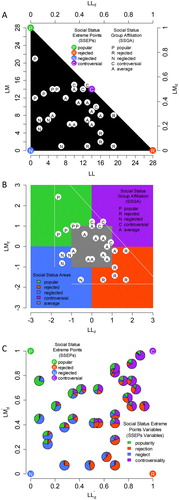
Within-class standardization: class-norm-referenced interpretation

Within-class standardized indegrees are needed for the CD procedure. It is often claimed that within-class standardization is done to control for differences in class size (Bukowski, Cillessen, and Velásquez 2012; Cillessen 2011; Coie, Dodge, and Coppotelli 1982; Veldman and Sheffield 1979). This misbelief shall be illustrated with a simplistic example of the indegrees of two different classes of the same class size (N = 8):

• Class A: 1, 1, 2, 2, 3, 3, 4, 4

• Class B: 0, 0, 1, 1, 2, 2, 3, 3

For both classes (A and B), within-class standardization leads to the same result (–1.25, –1.25, –0.42, –0.42, 0.42, 0.42, 1.25, 1.25). Numerically equal indegree values from two different classes of the same class size correspond with different within-class standardized indegree values (for example, class A: 2 → –0.42; class B: 2 → +0.42). This example shows that within-class standardized indegrees are not even coherently interpretable across classes of the same class size. Within-class standardization takes only the class-specific mean and class-specific variance into account. A non-zero LM_z or LL_z value represents a deviation from the class average (a deviation with respect to one class-specific standard deviation).² Therefore, within-class standardization of indegrees provides a class-norm-referenced interpretation. The ancillary effect of within-class standardization is that between-class differences in means and variances are entirely eliminated, i.e. all class means are forced to be zero and all class-specific variances are forced to be one.

Social status group affiliation (SSGA)

Using the CD classification procedure, children are classified into the different social status groups on the basis of within-class standardized indegrees. Additionally, a social preference score (SP_z: within-class standardized difference between LM_z and LL_z) and a social impact score (SI_z: within-class standardized sum of LM_z and LL_z) are required for social status group definition (for more details, see Coie and Dodge 1983). Decision rules (which are displayed with relational and logical operators) are subsequently applied to assign children to the social status groups (SSGA):

• Popular: LM_z > 0 & LL_z < 0 & SP_z > +1

• Rejected: LM_z < 0 & LL_z > 0 & SP_z < –1

• Neglected: LM_z < 0 & LL_z < 0 & SI_z < –1

• Controversial: LM_z > 0 & LL_z > 0 & SI_z > +1

Under consideration of these decision rules, the SSGA is determined by (standard) deviations around the class means of LM_z, LL_z, SP_z, and SI_z. Coie and Dodge (1983) advocate including all remaining children (who could not be assigned to a particular social status group by the abovementioned decision rules) in the average group. The resulting social status groups can be represented approximately as areas within a two-dimensional space (Figure 1(B)). Under the guidance of the CD classification procedure, the majority of children in the exemplary class are classified as average, whereas a few children are classified as popular, rejected, neglected, or controversial (Figure 1(A and B)). Since some children are peripheral within particular status groups or are even on the border between two or three different groups, the strict categorical classification appears to be an insufficient (crude) characterization of a child’s social status within the peer group.

Sociometric sample space: misdetection of controversial children

Within-class standardized indegrees suggest that the sociometric sample pace is a square (Figure 1(B)), and this opinion is further supported by square visualizations of the sociometric sample space (Coie, Dodge, and Coppotelli 1982; DeRosier and Thomas 2008; Košir and Pečjak 2005). In fact, however, the sociometric sample space is a triangle (Figure 1(A)) because, for any given child, the sum of both indegrees is less than or equal to the number of peers in the class minus one, i.e. less than or equal to the maximum number of receivable nominations per child (LM + LL ≤ MAX). This triangular structure remains mostly unaffected by within-class standardization of the indegrees. Consequently, the intersection of the triangular sample space and the controversial social status area is relatively small (Figure 1(B)). Due to this small intersection, the CD procedure is prone to failure in the identification of controversial children. Additionally, high SI_z values (SI_z > +1: condition for controversial group; SI_z: within-class standardized sum of LM_z and LL_z) are not likely because it is not likely to observe high LM_z and LL_z values concurrently (because the sum of both indegrees is less than or equal to the maximum number of receivable nominations per child: LM + LL ≤ MAX). These mathematical limitations correspond to the frequently observed small number of children in the controversial status group.

Class-norm-referenced interpretation: stability issues

The class-norm-referenced interpretation of the within-class standardized indegrees is also reflected in the SSGA. For example, a child classified as controversial is controversial with respect to the class norm, i.e. with respect to the centroid of the within-class standardized sociometric data (LL_z: 0, LM_z: 0). Practically, a child’s SSGA is strongly dependent on the indegrees of the other classmates. A child with high indegree values (for example, LM: 9, LL: 9) might have been classified as controversial in one class, while in another class he or she might have been classified as average (a class in which it is normal to have high indegree values, i.e. a class in which the norm is defined by high indegree values). Hence, the SSGA is not coherently interpretable across classes, i.e. the meaning of the state of being popular, rejected, neglected, controversial, or average might vary substantially across classes. If just one child receives one fewer or one more nomination, this will result in a shift of the sociometric centroid (i.e. shift of the class norm), as well as in a change of the bivariate distribution (LM and LL), and can therefore likewise result in a change of the distribution of the children over the status groups. Thus, stability of social status groups is sensitive to intraindividual variations of the indegrees. Hence, on the one hand, the stability of social status groups can have a substantive source (Cillessen, Bukowski, and Haselager 2000) and, on the other hand, the stability can also be attributed to the class-norm-referenced point of view on the sociometric data (i.e. attributed to within-class standardization).

Social status extreme points procedure (SSEPs procedure)

Social status extreme points (SSEPs)

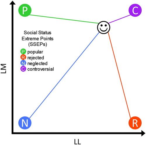
In terms of bivariate sociometric data (LL and LM), the positions of the SSEPs can be displayed in a schematic scatter plot (Figure 2: The sociometric sample space is visualized as a square for illustrative purposes only, though we have shown that the sample space is in fact a triangle). The four corners of the plot mark the hypothesized SSEPs, which are theoretical (not necessarily observed) extreme points of the sociometric data. The smiley in Figure 2 represents one child, i.e. one data point (along with the distances from the SSEPs). The coordinates of the SSEPs represent social status extreme types of children who are most popular (liked by all, disliked by no one), most rejected (liked by no one, disliked by all), most neglected (liked as well as disliked by no one), and most controversial (liked as well as disliked by half of the peers). The main idea of the SSEPs procedure is to describe each child in a peer group in terms of his or her closeness to the SSEPs. Thus, the shorter the distance between a child and a particular SSEP, the more appropriate is the corresponding social status description (degree of adaptation to a particular SSEP). For example, the child (smiley in Figure 2) is quite close to the controversial SSEP and is therefore highly controversial within the peer group. Hence, an intraindividual variation of the LM value and/or LL value can also be conceptualized as a deviation from or adaptation to each and every SSEP. This elaboration shows the multidimensional nature of a child’s social status. By extension, children who do not fit in exactly with one hypothesized SSEP can be represented as mixtures of all four SSEPs.³ This individual mixture is deducible from a child’s (data point’s) distance (Euclidean distance) from each and every SSEP. Furthermore, the average social status is located in the centre of the sociometric data (around the means of LM and LL) and is therefore hardly an extreme point and is omitted in the calculation of the SSEPs variables. The state of being average is a function/combination of the four SSEPs. Hence, the average social status is a mixture of the other SSEPs, i.e. an average child is equally popular, rejected, neglected, and controversial (25% popular, 25% rejected, 25% neglected, and 25% controversial).

Figure 2. SSEPs in a schematic scatter plot (LL and LM). The smiley represents one child/data point (along with the distances from the SSEPs).

Ego densities: criterion-referenced interpretation

For the localization of the SSEPs, we will not use the within-class standardized indegrees but rather a social network index, namely, the ego density (Wasserman and Faust 1994, 179). The ego density is simply the ratio of the indegree (received nominations, i.e. LM or LL) of a child to the maximum number of receivable nominations per child (ego density = indegree / MAX). So, the ego density interval is [0, 1]. This interval offers a criterion-referenced interpretation of the ego density (proportion of the maximum number of receivable nominations per child; 0: no nominations received; 1: all possible nominations received) instead of the class-norm-referenced interpretation of the within-class standardized indegree (deviation from the indegree class average). An additional advantage of the ego densities over the within-class standardized indegrees is that the ego density transformation does not entirely eliminate between-class differences in means and variances⁴, i.e. class-specific means and variances are not forced to be zero (M) and one (SD). The ego densities (LL_d and LM_d) are plotted in Figure 1(A) (notational exemplary school class). The SSEPs are theoretical (not necessarily observed) extreme points of the bivariate distribution of LL_d and LM_d. Thus, the coordinates of the SSEPs are determined by the semantics of the social status labels: popular (disliked by no one, liked by all; LL_d: 0, LM_d: 1), rejected (disliked by all, liked by no one; LL_d: 1, LM_d: 0), neglected (both disliked and liked by no one; LL_d: 0, LM_d: 0), and controversial (both disliked and liked by half of the peers; LL_d: 0.5, LM_d: 0.5). So, the SSEPs (popular, rejected, neglected) are the vertices of an isosceles right triangle (cathetus length of one), whereas the controversial SSEP is the midpoint of the hypotenuse of this triangle (Figure 1(A) and Figure 3(A)). Hence, the sociometric sample space is a triangle (as mentioned above). All children (data points) will be located in this isosceles right triangle.

Figure 3. Sociometric sample space. (A): Isosceles right triangle (LL_d and LM_d). (B): Unit square (LL_d′ and LM_d′).

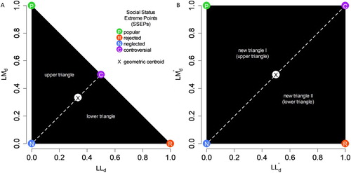
Affine transformation of sociometric sample space

The shorter the distance between a data point and a particular SSEP, the more appropriate is the corresponding social status description for the given data point. Unfortunately, the isosceles right triangle is a biased sample space, i.e. for all possible data points in the triangle, the average distance to the controversial SSEP is the lowest. This bias is due to the fact that the distances between the SSEPs and the geometric centroid of the isosceles right triangle are not equidistant (the controversial SSEP is the closest to the centroid), i.e. the isosceles right triangle is a centroid asymmetric sample space. To realize an unbiased representation of the distances between the data points and the SSEPs, it is necessary to transform the triangle into an unbiased sample space. To be unbiased, the sample space should satisfy the following condition: The distances between the SSEPs and the geometric centroid are all equidistant, i.e. a centroid symmetric sample space (e.g. square). This can be achieved by an affine transformation: Any triangle can be transformed into any other triangle (Brannan, Esplen, and Gray 2012, 89). The altitude to the hypotenuse divides the isosceles right triangle into two smaller triangles (Figure 3(A)). These two smaller triangles (upper and lower triangles) can be used to construct a unit square. The vertices of the upper triangle, (0, 1), (0.5, 0.5), and (0, 0), shall be mapped to the vertices (0, 1), (1, 1), and (0, 0), which form a new triangle. Any arbitrary point of the upper (old) triangle (LL_d, LM_d) will be mapped to the new triangle (LL_d′, LM_d′) by (new data points = vertices of new triangle * vertices of old triangle^–1 * old data points):$\left(\begin{array}{c}{\mathrm{L}\mathrm{L}}_{\mathrm{d}}^{{}^{\mathrm{\prime }}}\\ {\mathrm{L}\mathrm{M}}_{\mathrm{d}}^{{}^{\mathrm{\prime }}}\\ 1\end{array}\right)=\left(\begin{array}{ccc}0& 1& 0\\ 1& 1& 0\\ 1& 1& 1\end{array}\right){\left(\begin{array}{ccc}0& 0.5& 0\\ 1& 0.5& 0\\ 1& 1& 1\end{array}\right)}^{\text{–}1}\left(\begin{array}{c}\mathrm{L}{\mathrm{L}}_{\mathrm{d}}\\ \mathrm{L}{\mathrm{M}}_{\mathrm{d}}\\ 1\end{array}\right)$

In the above equation, all matrices are augmented with an extra row of ones (last row) and all vectors are augmented with ones at the end. The same affine transformation is done with the vertices of the lower triangle: (1, 0), (0.5, 0.5), and (0, 0). These vertices shall be mapped to the vertices (1, 0), (1, 1), and (0, 0), which form another new triangle, by:$\left(\begin{array}{c}{\mathrm{L}\mathrm{L}}_{\mathrm{d}}^{{}^{\mathrm{\prime }}}\\ {\mathrm{L}\mathrm{M}}_{\mathrm{d}}^{{}^{\mathrm{\prime }}}\\ 1\end{array}\right)=\left(\begin{array}{ccc}1& 1& 0\\ 0& 1& 0\\ 1& 1& 1\end{array}\right){\left(\begin{array}{ccc}1& 0.5& 0\\ 0& 0.5& 0\\ 1& 1& 1\end{array}\right)}^{\text{–}1}\left(\begin{array}{c}\mathrm{L}{\mathrm{L}}_{\mathrm{d}}\\ \mathrm{L}{\mathrm{M}}_{\mathrm{d}}\\ 1\end{array}\right)$

Both newly constructed triangles form a unit square (Figure 3(B)). With this two-step affine transformation, the controversial SSEP (LL_d: 0.5, LM_d: 0.5) is mapped to the point (LL_d′: 1, LM_d′: 1). The other SSEPs remain unchanged. Now, all SSEPs are the vertices of a unit square (Figure 1(C) and Figure 3(B)). Hence, all data points of the isosceles right triangle are now located in the unit square. The advantage of the affine transformation (over the within-class standardization) is that it preserves collinearity (bivariate transformation), i.e. the geometric centroid of the isosceles right triangle is mapped to the geometric centroid of the unit square, which allows an unbiased representation of the distances between the data points and the SSEPs, since the distances of the SSEPs from the geometric centroid of the unit square are all equidistant (centroid symmetric sample space).

It should be mentioned that if the class size (N) is even, then the maximum number of receivable nominations per child (MAX) is odd. In that case, it is not possible to be both liked and disliked by half of the peers (MAX / 2 is not an integer). Consequently, if MAX is odd, then the controversial SSEP is not the midpoint of the hypotenuse of the isosceles right triangle. In that case, the controversial SSEP will be located (just off the midpoint of the hypotenuse) at the altitude of the isosceles right triangle (LL_d: [MAX / 2–0.5] / MAX, LM_d: [MAX / 2–0.5] / MAX). So, if MAX is odd, then the triangular sample space has a notch (Figure 4). To ensure a triangular sample space, this notch needs to be filled, i.e. the controversial SSEP (LL_d: [MAX / 2–0.5] / MAX, LM_d: [MAX / 2–0.5] / MAX) needs to be mapped to the midpoint of the hypotenuse (LL_d: 0.5, LM_d: 0.5). The data points between the neglected SSEP and the notch are moved towards the notch via affine transformation. Following this, the isosceles right triangle is mapped to the unit square (as mentioned above). The R code (R Core Team 2018) to perform the affine transformations is available in the online supplementary material.

Figure 4. Notched isosceles right triangle (sociometric sample space if the class size [N] is even). The coordinates of the controversial SSEP are (LL_d: [MAX / 2–0.5] / MAX, LM_d: [MAX / 2–0.5] / MAX), where MAX is the maximum number of receivable nominations per child (MAX = N – 1).

Social status extreme points variables (SSEPs variables)

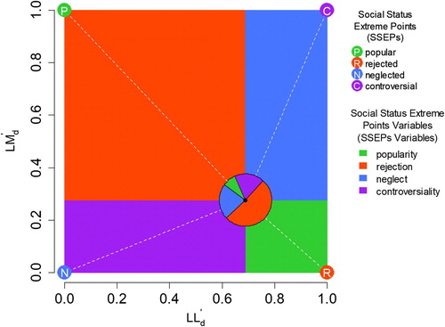
The affine transformed ego densities (LM_d′ and LL_d′) are used to determine the distances between the children (data points) and the SSEPs. However, the distances between a data point and the SSEPs can be represented approximately by rectangular areas (social status areas). Each data point divides the unit square into four rectangular areas, as shown for one particular data point (along with the data point’s distances from the SSEPs) in Figure 5. Each area corresponds with one SSEP (the corresponding areas and SSEPs diagonally opposite each other). Hence, the smaller the distance between a data point and a particular SSEP, the larger the corresponding social status area. If a child received no LL and a few LM nominations, the child’s distance to the controversial SSEP would indicate a certain degree of controversiality. But one cannot be controversial (liked and disliked by many) if one did not receive any LL nominations. In any case where LL equals zero, the controversial area will likewise be zero (no controversiality). Therefore, using the areas (instead of the distances) is more beneficial because the sum of the four areas is always one (uniform interpretation), whereas the sum of the four distances differs across data points. Thus, the areas are interpretable as fractions. These fractions are the variables newly introduced here (SSEPs variables): popularity, rejection, neglect, and controversiality. Each fraction f_ij can be understood as the degree of adaptation of child i to the SSEP j (where i = 1, … , N, j = {popular (1), rejected (2), neglected (3), controversial (4)}, and f_ij satisfies f_ij ≥ 0 and ${\mathrm{\Sigma }}_{\mathrm{j}=1}^{\mathrm{j}=4}$ f_ij = 1). The larger the fraction, the more appropriate is the corresponding social status description for the given child. With these fractions, all the observed data points (children) are representable as mixtures of the SSEPs. This mixture is representable as a pie chart, as is shown for the children in the exemplary school class in Figure 1(C) and for one particular child (along with the child’s distances from the SSEPs) in Figure 5. The last-mentioned child is 8% popular (popularity), 51% rejected (rejection), 22% neglected (neglect), and 19% controversial (controversiality) within the peer group (Σ = 100%). The R code (R Core Team 2018) for calculating the SSEPs variables is available in the online supplementary material.

Figure 5. The pie chart represents the SSEPs variable values of one child (exemplary school class). The distances (dotted white lines) between the data point (child) and the SSEPs can be approximately represented by rectangular areas. The centre of the pie chart (data point/child) divides the unit square into these four rectangular areas (coloured areas). Each social status area corresponds with one SSEP (the corresponding areas and SSEPs diagonally opposite each other).

In general, the popular and rejected SSEPs are opposite extreme points (centroid-symmetric). Consequently, if a child is close to the popular SSEP, then he or she is inevitably far away from the rejected SSEP (the distances are not completely determined by each other, but they do show a strong negative association: r = –.82; exemplary school class). Hence, a child with a high degree of popularity will more likely experience a low degree of rejection. The same is true for the association between neglect and controversiality (the neglected and controversial SSEPs are likewise opposite extreme points; correlation of distances: r = –.97). Considering the areas instead of distances, however, the popularity is less more determined by the rejection (r = –.73), and the neglect is less more determined by the controversiality (r = –.86). Two adjacent (non-opposite) social status areas (popularity/controversiality, controversiality/rejection, rejection/neglect, or neglect/popularity) are needed to completely determine the remaining social status areas. However, an intraindividual variation in one particular SSEPs variable entails a variation in all the other SSEPs variables. Thus, to avoid determinism and multicollinearity, each SSEPs variable could be considered individually (for example, as a predictor in a regression model).

At any rate, it should be kept in mind that different nomination criteria are used in sociometric assessment, for example, ‘Name the classmates next to whom you like to sit the most/least?’ (Krull, Wilbert, and Hennemann 2014), ‘Which three classmates would you like the most/least to play with during break time?’ (Mamas 2012), or, as originally proposed by Coie and Dodge (1983), ‘Name three classmates whom you like most/least’. Therefore, interpretations of social status information should always be done with respect to the type of nomination criteria in use. Admittedly, if one is interested in criterion-referenced categorical social status information, then one can still use arbitrary cutoff values for the SSEPs variables, for example, children are neglected if neglect > 75%.

Part 2: Empirical demonstration

In this part we would like to demonstrate the performance of the two methods (CD procedure and SSEPs procedure). For this we will use empirical data. Furthermore, we also examine the agreement between SSGA and SSEPs variables.

Method

Sampling procedure and participants

Data was collected in six German elementary schools in the federal state of Brandenburg in rural areas and small towns (population < 23,000). Grades 3–6 were included in the study. Written and informed consent was obtained from parents/legal guardians of the children. The study was approved by the Federal Ministry of Education of Brandenburg (approval criteria: compliance with data protection regulations and educational relevance of research). Data collection took place at the end of the first semester of the 2015/16 school year.

Three to seven classes (Mdn = 5) participated per school, for a total of 28 classes. The distribution of the classes over the grades is nearly equal (in each case, five classes in grades three and four as well as six classes in grades five and six). The median class size is 19 (Min = 13, Max = 25). The sample consists of 400 children in total. The median age of the children is 10 (Min = 7, Max = 12). The mean proportion of boys per class is 48% (SD = 16%). However, sociometric data is available on 316 children. Missing data is due to no parental consent (47 children, 11.75%) and absence of children during class, i.e. absence during data collection (37 children, 9.25%). For more than half of the classes, complete data is available on more than 80% of the children in a class (participation rate per class: Min = 26%, Q₁ = 75%, Mdn = 84%, Q₃ = 87%, Max = 100%). In this context, it is worth mentioning that an acceptable reliability of sociometric nominations (Cronbach’s α > .80) can be shown even with small participation rates (participation rate per class > 10%, Marks et al. (2013)).

Measures

Sociometry. A peer nomination method was used to collect the sociometric data. Nomination questionnaires were handed out to all children during class. The names of all classmates were listed on each page of the two-page questionnaire. Children were instructed to mark the peers with whom they like to play (LM, first page) and those with whom they do not like to play (LL, second page). Written and verbal instruction was accompanied by an emoticon on each page of the questionnaire (like to play: , do not like to play: ). Children were explicitly informed that they were also allowed to nominate none of their peers or as many peers as they liked (on each page) (unlimited peer nomination). For a discussion of the advantages and disadvantages of limited and unlimited nominations (e.g. limited nominations force children to be more selective and are thus more valid, but unlimited nominations provide more ecologically valid data), see Gommans and Cillessen (2015). Although the authors of the CD procedure (Coie and Dodge 1983) originally proposed the use of limited nominations, the unlimited peer nomination approach is widely used in conjunction with social status group classification procedures (Krull, Wilbert, and Hennemann 2014; Smith, Hubbard, and Laurenceau 2011). The resulting indegrees (LM and LL) were used to define a child’s SSGA (Coie and Dodge 1983) and SSEPs variables (as mentioned above). The R code (R Core Team 2018) for calculating the SSEPs variables is available in the online supplementary material.

Statistical analysis

The variables of main interest (SSGA and SSEPs variables) will be described in a univariate manner. The agreement between the SSGA and SSEPs variables will be demonstrated by regression analyses (SSEPs variables regressed on SSGA). With respect to the nested data structure (children within classes), all regression models are linear mixed effects (ME) models (alias multilevel or hierarchical models), i.e. random intercept only models or random intercept and slope models (Bates et al. 2015). All statistical analyses were conducted in R 3.3.2 (R Core Team 2018). Additional R packages were used to fit ME regression models (package lme4; Bates et al. 2015) and calculate marginal R² (package MuMIn, Barton 2016).

Results

Social status group affiliation (SSGA)

The distribution of the children over the social status groups is shown in a scatter plot of LL_d and LM_d (Figure 6(A)) and in a scatter plot of LL_z and LM_z (Figure 6(B)). The majority of the children are classified as average (203 children, 64.24%). There are a few more rejected children (55 children, 17.40%) than popular children (46 children, 14.56%). Since the set of data points (LL_z and LM_z) is not very noisy, just a minority of the children are classified as neglected (11 children, 3.48%) or controversial (1 child, 0.32%). The proportion of children in the different social status groups varies across classes (popular: SD = 8%, rejected: SD = 10%, neglected: SD = 5%, average: SD = 11%), whereas neglected children are present in just 8 classes and popular children are not present in 3 classes. Since it is not very useful to make any statistical statement about one child, the controversial child is omitted from further analyses (agreement analyses).

Figure 6. Main sample (N = 316 children). (A) Indegrees (LL and LM) and ego densities (LL_d and LM_d). The black isosceles right triangle represents the sociometric sample space. (B) Within-class standardized indegrees (LL_z and LM_z). Cutoffs for social status areas (LL_z and LM_z): ± 1 SD and ≶ 0. (C): Affine transformed ego densities (LL_d′ and LM_d′). Children’s SSEPs variable values are represented by pie charts.

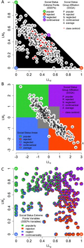
Social status extreme points variables (SSEPs variables)

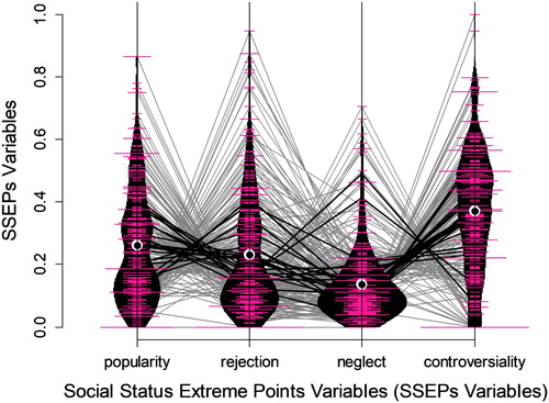
For each SSEPs variable, we will report the intercept (b₀) of a random intercept only model (no predictors; grouping variable: class membership) and the intraclass correlation coefficient (ICC). b₀ is interpretable as the weighted average across all classes. The ICC reflects the dependence between the variance in the particular SSEPs variable and the class membership. Additionally, children’s SSEPs variable values are represented by pie charts (Figure 6(C)). The distribution of each SSEPs variable and the corresponding parallel coordinates are shown in Figure 7. The children have on average the highest degree of controversiality (b₀ = .36), followed by popularity (b₀ = .27), rejection (b₀ = .23), and neglect (b₀ = .14). Most of the variance in the neglect can be explained by the class membership (ICC = .71). The dependence between the variance (in the SSEPs variables) and the class membership is not that strong in the cases of the remaining SSEPs variables (controversiality: ICC = .30, popularity: ICC = .20, rejection: ICC = .13).

Figure 7. Distributions (mirrored densities and histograms) together with means (black points) of the SSEPs variables. Parallel coordinates: Intraindividual polylines (gray: children, black: class average), each line with four vertices, each vertex represents one SSEPs variable.

Agreement between social status group affiliation (SSGA) and social status extreme points variables (SSEPs variables)

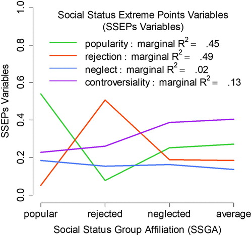
The average SSEPs variable values (by SSGA) are represented in Figure 8 (each SSEPs variable is regressed on the SSGA). Children classified as popular show a high average degree of popularity and a low average degree of rejection (content agreement). Children classified as rejected show a high average degree of rejection and a low average degree of popularity (content agreement). Children classified as neglected show a low average degree of neglect and a high average degree of controversiality (content disagreement). The popular, rejected, neglected, and average children show a similar average degree of neglect and are thus not dissociable on the basis of the neglect. The statistical agreement between a particular SSEPs variable and SSGA can be described by the marginal R² (variance in a particular SSEPs variable explained by fixed effects, i.e. by SSGA, see Figure 8) (Johnson 2014). The agreement between popularity/rejection and SSGA is respectable (popularity: marginal R² = .46, rejection: marginal R² = .49). The agreement between controversiality and SSGA is poor (marginal R² = .13). The poorest agreement is found between neglect and SSGA (marginal R² = .02).

Figure 8. Agreement between SSGA and SSEPs variables. The average SSEPs variable values (by SSGA) are represented by the vertices of the lines. The average SSEPs variable values derive from ME regression models (each SSEPs variable is regressed on the SSGA; grouping variable: class membership; the SSGA is a dummy variable). Since it is not very useful to make any statistical statements about one child, the controversial child is omitted from the data.

Discussion

Social status classification shortcomings

Shortcomings in social status classification have been highlighted using the example of the CD procedure (Coie and Dodge 1983). Since the within-class standardized indegrees suggest that the sociometric sample pace is a square (but in fact it is a triangle), the CD procedure is prone to failure in identification of controversial children (just one child from the main sample is classified as controversial, while the SSEPs variable of controversiality is on average the highest). Also, the number of neglected children identified by the CD procedure is marginal (11 children from the main sample). However, it seems to be a common but doubtful practice to modify classification rules in order to increase the number of neglected children in a sample (Rubin et al. 1989, 96):

[…] the standardized score approach popularized by Coie and Dodge and their colleagues (e.g. Coie, Dodge, and Coppotelli 1982) has been most often employed in recent sociometric research, yet the specific criteria used to identify sociometric subgroups differs from one research report to the next. This is particularly true in the case of neglected children where criteria appear to vary, in part, as a result of efforts to increase sample size.

The distribution of sociometric data is often skewed or zero-inflated, and within-class standardization of not normally or asymmetrically distributed data can be somewhat misleading (especially when interpretation across classes is the goal). With this standardization, the social reality (between-class differences in means and variances) is removed from the sociometric data. This kind of vague social status information might be problematic in the prediction of child behaviour (e.g. internalizing behaviour). These problems arising through within-group standardization of nested data (e.g. children within classes) have been discussed earlier by Moeller (2015) and Velásquez, Bukowski, and Saldarriaga (2013). Thus, the elimination of between-class differences (within-group standardization) is not recommendable, especially when interpretation across classes is the goal. Besides, social status observations are dependent on each other within classes. In the case of dependency of observations within classes, the data analytic ignorance of the nested data structure may lead to erroneous conclusions (Hill and Rowe 1996), for example, in the prediction of child behaviour. Except within-class standardization of the sociometric data, none of the studies cited thus far concerning the internalizing behaviour of neglected children (Boivin, Poulin, and Vitaro 1994; Burton and Krantz 1990; Cantrell and Prinz 1985; Cassidy and Asher 1992; Harrist et al. 1997; Hecht, Inderbitzen, and Bukowski 1998; Kupersmidt and Patterson 1991) has made any data analytic efforts to take the nested data structure into account. Thus, contradictory evidence concerning the association between neglected social status and internalizing behaviour could potentially be attributed to the data analytic ignorance of the nested data structure. One way to consider the nested data structure in social network data analysis is to apply the ME regression approach (alias multilevel or hierarchical regression) (Snijders 2016), for example, in the prediction of neglected children’s internalizing behaviour. Anyway, eliminating between-class differences through within-class standardization (CD procedure) while using a tool to account for between-class differences (ME regression) would be somewhat conflicting. Therefore, the CD procedure is not really compatible with the ME regression approach.

Overcoming the shortcomings: social status extreme points procedure (SSEPs procedure)

To overcome the shortcomings related to social status classification procedures, we have introduced the SSEPs procedure. This procedure describes a child’s social status in terms of his or her adaptation to each and every SSEP (multidimensionality). The SSEPs are social status extreme types (for example, an absolutely neglected child). Thus, the continuous SSEPs variables offer a criterion-referenced interpretation and are intuitively understandable (the degree of adaptation to each and every SSEP). Advantageously, between-class differences in the sociometric data remain mostly unaffected by the SSEPs procedure which makes the SSEPs variables suitable with the ME regression approach. An important difference between the two social status procedures is that the SSGA offers a class-norm-referenced interpretation, whereas the SSEPs variables offer a criterion-referenced interpretation. Concerning the empirical main sample, there is generally speaking a respectable agreement between the two methods. However, the agreement between the class-norm-referenced classification of neglected children and the criterion-referenced measure of neglect is very poor, which means that the state of being neglected is represented in two different ways by the two social status procedures. Future research may examine whether the SSEPs procedure could help to better understand the internalizing behaviour of neglected children.

Limitations and conclusions

In recent decades, many approaches have been developed to quantify a child’s social status. There may be no best method to use, rather, the optimal choice depends on one’s study population and study aims. When choosing a social status procedure, it is also important to know the strengths and weaknesses of the different methods (as described in the paper at hand). It should be kept in mind that every kind of calculation of social status information is just a recalculation of the two-dimensional sociometric information (LL and LM). We do not claim to have presented a perfect way to quantify a child’s social status. For example, the multicollinearity of the SSEPs variables can be a problem for statistical analyses. On the other hand, the SSEPs procedure offers many innovations, e.g. continuous metric, multidimensional information, and criterion-referenced interpretation. The reader has to decide whether and to what extent the SSEPs procedure offers an advantage (to investigate a specific research question) and whether the method proposed here or only certain (adapted) elements are used. Last but not least, ethical and ecological standards should also be taken into account when applying sociometric methods (Avramidis et al. 2016; Child and Nind 2013). The usage of negative peer nominations (LL) can reinforce negative peer relations. Simplistic sociometric peer nominations do not entirely reflect the complexity of social peer relations.

Conflict of interest

The authors declare that the research was conducted in the absence of any commercial or financial relationships that could be construed as a potential conflict of interest.

Acknowledgments

We thank Lynn Scherreiks, Josephnie Gutsche, and Isabell Augustin for assistance with data collection and Miriam Balt, Marie-Luise Gehrmann, Jannis Bosch, Moritz Börnert-Ringleb, and the anonymous reviewers for comments that greatly improved the manuscript. We would also like to thank the teachers, students, and parents for their participation in this study.

Disclosure statement

No potential conflict of interest was reported by the authors.

ORCID

Pawel R. Kulawiak http://orcid.org/0000-0001-5939-4380

Notes

1 In the following, the term neglected refers to sociometrically neglected children (not to be confused with the term child neglect, which is normally used in the context of child poverty and abuse).

2 Within-class standardization would be an adjustment for class size, if the indegree increases strictly monotonically with the class size (the bigger the class, the more sociometric nominations received per child, i.e., a strictly monotonic increase of class size and of indegree class average), as well as if the indegree variance is also constant across classes (so that deviations from class averages would be coherently interpretable across all classes). These assumptions are not justifiable, because between-class differences (in means and variances) in the sociometric data are the rule and are usually not that strongly associated with the class size (main sample: LM regressed on class size, marginal R² = .02; LL regressed on class size, marginal R² = .17; marginal R² is concerned with variance explained by fixed effects [Johnson 2014], i.e., by class size).

3 Analogies to archetypal analysis (Cutler and Breiman 1994) are apparent.

4 The intraclass correlation coefficient (ICC) reflects the dependence between the variance in the sociometric data and the class membership (main sample: ICC_LL = .46, ICC_LLd = .37, ICC_LLz = .00, ICC_LM = .21, ICC_LMd = .21, ICC_LMz = .00).

References

- Asher, Steven R., and Kenneth A. Dodge. 1986. “Identifying Children Who Are Rejected by Their Peers.” Developmental Psychology 22 (4): 444–449. https://doi.org/10.1037/0012-1649.22.4.444.
- Avramidis, Elias, Vasilis Strogilos, Katerina Aroni, and Christina Thessalia Kantaraki. 2016. “Using Sociometric Techniques to Assess the Social Impacts of Inclusion: Some Methodological Considerations.” Educational Research Review, December. https://doi.org/10.1016/j.edurev.2016.11.004.
- Barton, Kamil. 2016. MuMIn: Multi-Model Inference. R Package Version 1.15.6. https://CRAN.R-project.org/package=MuMIn.
- Bates, Douglas, Martin Mächler, Ben Bolker, and Steve Walker. 2015. “Fitting Linear Mixed-Effects Models Using Lme4.” Journal of Statistical Software 67 (1): 1–48. https://doi.org/10.18637/jss.v067.i01.
- Boivin, Michel, François Poulin, and Frank Vitaro. 1994. “Depressed Mood and Peer Rejection in Childhood.” Development and Psychopathology 6 (03): 483. https://doi.org/10.1017/S0954579400006064.
- Brannan, David A., Matthew F. Esplen, and Jeremy Gray. 2012. Geometry. 2nd ed. Cambridge; New York: Cambridge University Press.
- Brown, Jeremy Roger Selwyn. 2015. Neglected Children: What Does It Mean to Be Not Noticed in School? Southampton: University of Southampton. https://eprints.soton.ac.uk/382660 /.
- Bukowski, William M., Antonius H. N. Cillessen, and Ana Maria Velásquez. 2012. “Peer Ratings.” In Handbook of Developmental Research Methods, edited by Brett Paul Laursen, Todd D. Little, and Noel A. Card, 211–228. New York: Guilford Press.
- Burton, Christine B., and Murray Krantz. 1990. “Predicting Adjustment in Middle Childhood From Early Peer Status.” Early Child Development and Care 60 (1): 89–100. https://doi.org/10.1080/0300443900600108.
- Cantrell, V. L., and Ronald J. Prinz. 1985. “Multiple Perspectives of Rejected, Neglected, and Accepted Children: Relation Between Sociometric Status and Behavioral Characteristics.” Journal of Consulting and Clinical Psychology 53 (6): 884–889. https://doi.org/10.1037//0022-006X.53.6.884.
- Cassidy, Jude, and Steven R. Asher. 1992. “Loneliness and Peer Relations in Young Children.” Child Development 63 (2): 350. https://doi.org/10.2307/1131484.
- Child, Samantha, and Melanie Nind. 2013. “Sociometric Methods and Difference: A Force for Good – or yet More Harm.” Disability & Society 28 (7): 1012–1023. https://doi.org/10.1080/09687599.2012.741517.
- Cillessen, Antonius H. N. 2011. “Sociometric Methods.” In Handbook of Peer Interactions, Relationships, and Groups, edited by Kenneth H. Rubin, William M. Bukowski, and Brett Paul Laursen, 82–99. New York: Guilford.
- Cillessen, Antonius H. N., William M. Bukowski, and Gerbert J. T. Haselager. 2000. “Stability of Sociometric Categories.” New Directions for Child and Adolescent Development 2000 (88): 75–93. https://doi.org/10.1002/cd.23220008807.
- Coie, John D., and Kenneth A. Dodge. 1983. “Continuities and Changes in Children’s Social Status: A Five-Year Longitudinal Study.” Merrill-Palmer Quarterly 29 (3): 261–282.
- Coie, John D., Kenneth A. Dodge, and Heide Coppotelli. 1982. “Dimensions and Types of Social Status: A Cross-Age Perspective.” Developmental Psychology 18 (4): 557–570. https://doi.org/10.1037/0012-1649.18.4.557.
- Crews, S. Dean, Hermine Bender, Clayton R. Cook, Frank M. Gresham, Lee Kern, and Mike Vanderwood. 2007. “Risk and Protective Factors of Emotional and/or Behavioral Disorders in Children and Adolescents: A Mega-Analytic Synthesis.” Behavioral Disorders 32 (2): 64–77.
- Cutler, Adele, and Leo Breiman. 1994. “Archetypal Analysis.” Technometrics 36 (4): 338–347. https://doi.org/10.2307/1269949.
- DeRosier, Melissa E., and James M. Thomas. 2003. “Strengthening Sociometric Prediction: Scientific Advances in the Assessment of Children’s Peer Relations.” Child Development 74 (5): 1379–1392. https://doi.org/10.1111/1467-8624.00613.
- DeRosier, Melissa E., and J. Thomas. 2008. System and Method for Performing Sociometric Data Collection and Analysis for the Sociometric Classification of Schoolchildren. Google Patents. https://www.google.com/patents/US7330823.
- Frederickson, N. L., and A. F. Furnham. 1998. “Sociometric Classification Methods in School Peer Groups: A Comparative Investigation.” Journal of Child Psychology and Psychiatry, and Allied Disciplines 39 (6): 921–933.
- Gommans, R., and A. H. N. Cillessen. 2015. “Nominating Under Constraints: A Systematic Comparison of Unlimited and Limited Peer Nomination Methodologies in Elementary School.” International Journal of Behavioral Development 39 (1): 77–86. https://doi.org/10.1177/0165025414551761.
- Harrist, Amanda W., Anthony F. Zaia, John E. Bates, Kenneth A. Dodge, and Gregory S. Pettit. 1997. “Subtypes of Social Withdrawal in Early Childhood: Sociometric Status and Social-Cognitive Differences Across Four Years.” Child Development 68 (2): 278. https://doi.org/10.2307/1131850.
- Hecht, D. B., H. M. Inderbitzen, and A. L. Bukowski. 1998. “The Relationship Between Peer Status and Depressive Symptoms in Children and Adolescents.” Journal of Abnormal Child Psychology 26 (2): 153–160.
- Hendrickx, Marloes M. H. G., Tim Mainhard, Sophie Oudman, Henrike J. Boor-Klip, and Mieke Brekelmans. 2016. “Teacher Behavior and Peer Liking and Disliking: The Teacher as a Social Referent for Peer Status.” Journal of Educational Psychology, https://doi.org/10.1037/edu0000157.
- Hill, Peter W., and Kenneth J. Rowe. 1996. “Multilevel Modelling in School Effectiveness Research.” School Effectiveness and School Improvement 7 (1): 1–34. https://doi.org/10.1080/0924345960070101.
- Hughes, Jan N., and Myung H. Im. 2016. “Teacher-Student Relationship and Peer Disliking and Liking Across Grades 1-4.” Child Development 87 (2): 593–611. https://doi.org/10.1111/cdev.12477.
- Johnson, Paul C. D. 2014. “Extension of Nakagawa & Schielzeth’s R2GLMM to Random Slopes Models.” Methods in Ecology and Evolution 5 (9): 944–946. https://doi.org/10.1111/2041-210X.12225.
- Košir, Katja, and Sonja Pečjak. 2005. “Sociometry as a Method for Investigating Peer Relationships: What Does It Actually Measure?” Educational Research 47 (1): 127–144. https://doi.org/10.1080/0013188042000337604.
- Krull, Johanna, Jürgen Wilbert, and Thomas Hennemann. 2014. “The Social and Emotional Situation of First Graders with Classroom Behavior Problems and Classroom Learning Difficulties in Inclusive Classes.” Learning Disabilities: A Contemporary Journal 12 (2): 169–190.
- Kupersmidt, Janis B., and Charlotte J. Patterson. 1991. “Childhood Peer Rejection, Aggression, Withdrawal, and Perceived Competence as Predictors of Self-Reported Behavior Problems in Preadolescence.” Journal of Abnormal Child Psychology 19 (4): 427–449. https://doi.org/10.1007/BF00919087.
- Laghi, Fiorenzo, Francesca Federico, Antonia Lonigro, Simona Levanto, Maurizio Ferraro, Emma Baumgartner, and Roberto Baiocco. 2016. “Peer and Teacher-Selected Peer Buddies for Adolescents With Autism Spectrum Disorders: The Role of Social, Emotional, and Mentalizing Abilities.” The Journal of Psychology 150 (4): 469–484. https://doi.org/10.1080/00223980.2015.1087375.
- Maassen, Gerard H., Henderien Steenbeek, and Paul van Geert. 2004. “Stability of Three Methods for Two-Dimensional Sociometric Status Determination Based on the Procedure of Asher, Singleton, Tinsley and Hymel.” Social Behavior and Personality: An International Journal 32 (6): 535–550. https://doi.org/10.2224/sbp.2004.32.6.535.
- Mamas, Christoforos. 2012. “Pedagogy, Social Status and Inclusion in Cypriot Schools.” International Journal of Inclusive Education 16 (11): 1223–1239. https://doi.org/10.1080/13603116.2011.557446.
- Marks, Peter E. L., Ben Babcock, Antonius H. N. Cillessen, and Nicki R. Crick. 2013. “The Effects of Participation Rate on the Internal Reliability of Peer Nomination Measures: Participation and Sociometric Reliability.” Social Development 22 (3): 609–622. https://doi.org/10.1111/j.1467-9507.2012.00661.x.
- McMullen, Jake A., Koen Veermans, and Kaarina Laine. 2014. “Tools for the Classroom? An Examination of Existing Sociometric Methods for Teacher Use.” Scandinavian Journal of Educational Research 58 (5): 624–638. https://doi.org/10.1080/00313831.2013.838694.
- Moeller, Julia. 2015. “A Word on Standardization in Longitudinal Studies: Don’t.” Frontiers in Psychology 6 (September). https://doi.org/10.3389/fpsyg.2015.01389.
- Newcomb, Andrew F., and William M. Bukowski. 1983. “Social Impact and Social Preference as Determinants of Children’s Peer Group Status.” Developmental Psychology 19 (6): 856–867. https://doi.org/10.1037/a0025399.
- Newcomb, Andrew F., William M. Bukowski, and Linda Pattee. 1993. “Children’s Peer Relations: A Meta-Analytic Review of Popular, Rejected, Neglected, Controversial, and Average Sociometric Status.” Psychological Bulletin 113 (1): 99–128. https://doi.org/10.1037/0033-2909.113.1.99.
- Pasta, J. David. 2009. “Learning When to Be Discrete: Continuous vs. Categorical Predictors.” In SAS Global Forum, edited by SAS Institute, 1–10. Cary, NC, USA.
- R Core Team. 2018. R: A Language and Environment for Statistical Computing. Vienna, Austria: R Foundation for Statistical Computing. https://www.R-project.org/.
- Rubin, Kenneth H., Shelley Hymel, Lucy Lemare, and Lynda Rowden. 1989. “Children Experiencing Social Difficulties: Sociometric Neglect Reconsidered.” Canadian Journal of Behavioural Science / Revue Canadienne Des Sciences Du Comportement 21 (1): 94–111. https://doi.org/10.1037/h0079775.
- Shaw, Dale G., Michael D. Huffman, and Mark G. Haviland. 1987. “Grouping Continuous Data in Discrete Intervals: Information Loss and Recovery.” Journal of Educational Measurement 24 (2): 167–173. https://doi.org/10.1111/j.1745-3984.1987.tb00272.x.
- Smith, Marissa, Julie A. Hubbard, and Jean-Philippe Laurenceau. 2011. “Profiles of Anger Control in Second-Grade Children: Examination of Self-Report, Observational, and Physiological Components.” Journal of Experimental Child Psychology 110 (2): 213–226. https://doi.org/10.1016/j.jecp.2011.02.006.
- Snijders, Tom A.B. 2016. “The Multiple Flavours of Multilevel Issues for Networks.” In Multilevel Network Analysis for the Social Sciences, edited by Emmanuel Lazega and Tom A.B. Snijders, 15–46. Cham: Springer International Publishing. https://doi.org/10.1007/978-3-319-24520-1.
- Terry, Robert, and John D. Coie. 1991. “A Comparison of Methods for Defining Sociometric Status among Children.” Developmental Psychology 27 (5): 867–880. https://doi.org/10.1037/0012-1649.27.5.867.
- Velásquez, Ana Maria, William M. Bukowski, and Lina Maria Saldarriaga. 2013. “Adjusting for Group Size Effects in Peer Nomination Data: Adjusting for Group Size Effects.” Social Development, June, 845–863. https://doi.org/10.1111/sode.12029.
- Veldman, Donald J., and John R. Sheffield. 1979. “The Scaling of Sociometric Nominations.” Educational and Psychological Measurement 39 (1): 99–106. https://doi.org/10.1177/001316447903900114.
- Wasserman, Stanley, and Katherine Faust. 1994. Social Network Analysis: Methods and Applications. Structural Analysis in the Social Sciences 8. Cambridge; New York: Cambridge University Press.
- Wentzel, Kathryn R., and Steven R. Asher. 1995. “The Academic Lives of Neglected, Rejected, Popular, and Controversial Children.” Child Development 66 (3): 754. https://doi.org/10.2307/1131948.