Defining and evaluating stability in early years assessment

ABSTRACT

Stability is an important underlying assumption in any form of assessment-supported decision-making. Since early years development is frequently described as unstable, the concept plays a central role in the discussion surrounding early years assessment. This paper describes stability as a set of assumptions about the way individual scores change over time. Here, an analytical framework developed by Tisak and Meredith, which can be used to evaluate these assumptions, is extended and applied to evaluate the stability of mathematics scores of 1402 children between kindergarten and third grade. Multilevel models are used to evaluate the assumption that each child has a unique individual growth rate, as well as the assumption that the ranking of children’s test scores is consistent over time. The results show that for a large proportion of the children, assuming unique individual growth rates leads to similar predictions as assuming that children develop at an equal pace. While individual differences in growth rate may provide relevant information, these differences only become apparent after several test administrations. As such, decisions should not be based on perceived stagnated or accelerated growth over a short period.

KEYWORDS:

• Stability
• assessment
• early years
• longitudinal

Most practical applications of educational assessment have an inherently predictive nature (Shepard 1997). This is because the decisions that assessment results are designed to support typically concern expected developmental outcomes in the near or more distant future. According to Cronbach, the ability of test results to improve inferences about future functioning validates their use in any decision-making process. He states that any decision is a choice between several courses of action and that the validity of a decision is ‘based on the prediction that the outcome will be more satisfactory under one course of action than another’ (Cronbach 1971, 448). Test results benefit educational decisions only to the extent that they improve the accuracy of predictions and, hence, reduce the number of incorrect decisions.

Likewise, the argument for the identification of children’s developmental problems using test scores is not based on current performance, but on the expectation that this performance reflects some unfavourable outcome in the future unless action is taken. Bracken and Walker (1997) describe this expectation as an assumption of the stability of the test score. Similarly, Kagan (1971) notes that stability permits early diagnoses by facilitating the prediction of future behaviour and, as such, determines the significance that can be placed on responses. A general definition of stability is given by Wohlwill (1973, 144), who equates stability with predictability in the following statement: ‘the predictability of an individual’s relative standing on behaviour Y at time t₂ from his relative standing on behaviour X at t₁.’ In terms of assessment: a test score is more stable if we can predict a child’s later test score from his/her early scores to a higher degree.

The term stability (or lack thereof) is frequently used in the literature on early years assessment. In a review on school readiness screenings, La Paro and Pianta (2000) conclude that instability may be the rule rather than the exception between preschool and second grade. Similarly, Nagle (2000) describes test scores in the early years as characteristically unstable. According to Nagle (2000), preschool children comprise a unique and qualitatively different population compared to school-aged pupils. Their rapid developmental change across various domains may be discontinuous and unstable, with highly diverse rates of maturation and spurts in development commonly observed in the preschool years. These distinguishing features in preschool development make preschool assessment a complex and challenging task (Bracken and Walker 1997; Nagle 2000). Additionally, while standardized testing is one of the most widely used means of evaluating children’s abilities (Dockrell et al. 2017; La Paro and Pianta 2000), standardized assessment settings are often new and unfamiliar for young children. Children’s relatively short attention spans, high levels of activity and distractibility, and a low sense of the significance of correctly answering questions at this age often mean that such tests are by no means an ideal context for assessing preschool children (Nagle 2000). These unique characteristics in development and test-taking behaviour may lead to the characteristically low stability of test scores in early years assessment (Nagle 2000).

While stability is a core concept in assessment-supported decision-making, particularly in early years assessment, a review of the literature on stability shows that the concept has many nuanced definitions that are often used interchangeably. The aim of this paper is to reconsider the meaning of stability and to extend an existing analytical framework that may be used to evaluate stability. Since mathematics is an important domain in early years development (Duncan et al. 2007) and crucial in decision-making processes in the transition to formal education (Mashburn and Henry 2004), the framework described is applied to evaluate the stability of the mathematics scores of 1402 children between kindergarten and third grade.

Defining stability

Wohlwill gives an account of at least four types of stability: strict stability, parallel stability, linear/monotonic stability and function stability.¹ Wohlwill (1973) defines stability primarily as an attribute of an individual’s developmental pattern, rather than as a characteristic of a trait or variable. Consequently, each type is defined by the predictability of an individual’s growth pattern. This predictability is characterized by two types of alterations that occur in development (Lerner, Lewin-Bizan, and Alberts Warren 2011): children change over time relative to themselves (intraindividual change); and children change over time relative to others (interindividual change).

Strict stability is defined as the absence of intraindividual differences (Hartmann, Pelzel, and Abbott 2011; Kagan 1980; Wohlwill 1980). According to this definition, behaviour is expected to remain unchanged over time. Consequently, interindividual differences are consistent over time. Strict stability is described by Kagan (1980, 31) as ‘persistence of a psychological quality as reflected in minimal rate of change in that quality over time’. In most forms of developmental assessment, this type of development is of little interest, as a change in behaviour is expected to occur. However, it may be important when evaluating ‘the role of early experience in laying down patterns of behaviour that remain unchanged subsequently.’ (Wohlwill 1973, 362).

Parallel stability is defined as the interindividual consistency of differences over time (Bornstein et al. 2014). Contrary to absolute invariance, intraindividual change may occur according to this definition (i.e. an individual’s behaviour or test score may change); however, each individual has the same expected growth rate. Similar to strict stability, it follows that interindividual differences are constant over time.

A less restricted form of stability is known as monotonic or linear stability, which assumes that both intra- and interindividual change may occur, while the interindividual rank order remains constant between time points (e.g. Bornstein, Brown, and Slater 1996; Bornstein, Hahn, and Haynes 2004; Bornstein and Putnick 2012; Kagan 1971; McCall 1981). This is also known as stability of rank order (Lerner, Lewin-Bizan, and Alberts Warren 2011). Examples of this type of stability include consistency of IQ scores or percentile ranks (Wohlwill 1973).

Finally, Wohlwill (1973, 361) describes function stability as ‘the degree of correspondence between an individual’s developmental function and some prototypic curve, derived either on empirical or theoretical grounds.’ While parallel stability assumes that the developmental function and its growth rates (i.e. growth parameters) are the same for each individual, this type of stability assumes that the function is the same across individuals, but the growth rates may differ between individuals. According to this type of stability, both intra and interindividual differences may occur, even in rank order.

Deviations from stability can occur in two forms (Rudinger and Rietz 1998): random changes from expected development or structural differences in growth. Random changes reflect uncertainty about a child’s ability due to factors that are unrelated to their intrinsic ability. For example, a child may have been sick or distracted during the test administration or had a particularly fortunate guessing streak. Structural differences, by contrast, indicate that the adopted assumption about the type of stability is incorrect and a different type of stability may better describe the development. What is considered to be random variation changes depending on assumptions about structural change. Individual differences in scores over time can lead to different conclusions depending on whether these differences are viewed as individual structural growth (e.g. assuming function stability), or random variations around an individual’s true ability (e.g. assuming strict stability). To evaluate the validity of such assumptions, we need to define the structural model of each type of stability.

An analytical framework to assess stability

Since the study of stability centres on individual development, any model used to evaluate stability must be specified at the individual level (Tisak and Meredith 1990). Coincidentally, this makes test-retest correlations (sometimes referred to as stability coefficients) inadequate as a measure of stability, because these coefficients cannot be disaggregated to the individual level (Asendorpf 1992). Moreover, correlations poorly differentiate between the distinct types of stability described above, which often leads to misinterpretations (e.g. Asendorpf 1992; Bornstein and Putnick 2012; Mroczek 2007). Indeed, a perfect correlation does not differentiate between the first three types, and an imperfect correlation may occur even when all observations are perfectly consistent with the latter two types.

Tisak and Meredith (1990) defined the first three types of stability proposed by Wohlwill (1973) using a structural equation model (SEM) for individual development, thereby making stability estimable and testable. Although their model provides a coherent and well-defined evaluative framework of stability, its application in scientific literature has thus far been limited. Since SEM is mathematically equivalent to the multilevel model (MLM), each stability type can be rewritten as a multilevel regression model. The naturally occurring hierarchies in educational contexts (e.g. test scores nested within students, students nested within schools) have made these models particularly prominent in educational research. Mroczek (2007) suggests that MLM may be more appealing when evaluating stability, as many researchers find it easier to conceive of individual growth curves than to envision change as the result of a latent intercept and slope. When, for the sake of simplicity, only one level of nesting is included, the MLM formulation for a construct Y of individual $i=1,2,\dots ,N$. at time t is:(1) $\begin{array}{cc}\mathrm{L}\mathrm{e}\mathrm{v}\mathrm{e}\mathrm{l}1:& Y_{it}={\text{β}}_{0i}+\sum _{k=1}^d{\text{β}}_{ki}\left(t\right)+R_{it}\\ \mathrm{L}\mathrm{e}\mathrm{v}\mathrm{e}\mathrm{l}2:& {\text{β}}_{0i}={\gamma }_{00}+U_{0i}\\ & {\text{β}}_{ki}={\gamma }_{1k}+U_{ki}\end{array}$(1) Here, the growth curve of eacindividual is described by an intercept${\text{β}}_{0i}$ and d time parameters ${\text{β}}_{ki}\left(t\right)$. Each of these parameters is the sum of a fixed part that all individuals have in common (${\gamma }_{00}$ and ${\gamma }_{1k}$) and a random part that is specific to each individual i ($U_{0i}$ and $U_{ki}$). Wle structural change for an individual is described by these two parts of the model, each observation has a residual $\left(R_{it}\right)$that describes random deviations from the expected outcome for individual i at time t. The individual parameters and residuals are assumed to be normally distributed, with an expected value of zero and variance ${\tau }_k^2$ and ${\sigma }^2$, respectively. The variance of the random intercept ${\tau }_0^2$ can be interpreted as the degree of interindividual differences in the starting scores of children, while the variance of the random slope ${\tau }_1^2$ is a measure of the interindividual differences in growth rates. The variance of the residuals ${\sigma }^2$ can be viewed as the degree of random variation left after the structural parts of the model are accounted for.

Extension of the model to include a third level (e.g. school) is possible by including a subscript j that identifies each school and defining ${\gamma }_{00j}$ as the sum of a fixed part ${\delta }_{000}$ and a random part $V_{00k}$ that is specific to each school (e.g. Snijders and Bosker 2012).

Table 1 expresses each stability type in an MLM equation for a simple linear situation (d = 1; one-time parameter), along with providing a graphical representation of the model. Under the assumption of strict stability, there is variation between individuals ($U_{0i}$) within a common intercept. However, all intraindividual variation is assumed to be random ($R_{it}$) as $Y_{it}$ is not a function of time. Parallel stability adds a growth term that is assumed to be the same for each individual (${\text{β}}_1$). Linear/monotonic stability can be modelled by allowing this growth term to vary between individuals $\left(U_{1i}\right)$ but restricting it as a linear or monotonic function of $U_{0i}$. The analogous SEM formulations are presented by Tisak and Meredith (1990, 394). As they noted, each type of stability is a less restricted version of the previous model (i.e. the models are nested). Their framework can be extended to include function stability by omitting the restricted assumption that $U_{1i}$ needs to be dependent on $U_{0i}$. This allows individual growth parameters to vary freely between children, while keeping the growth function the same for each child.

Table 1. Types of stability and corresponding (linear) multilevel models and assumptions.

Type	Model	Model assumptions	Graphical representation
Strict stability: Intraindividual differences are absent	$Y_{it}={\text{β}}_{0i}+R_{it}$ ${\text{β}}_{0i}={\gamma }_{00}+U_{0i}$	$U_{0i}\sim N\left(0,{\tau }_0\right)$ $R_{it}\sim N\left(0,\sigma \right)$
Parallel stability: Intraindividual differences are the same for each individual	$Y_{it}={\text{β}}_{0i}+{\text{β}}_{1}t+R_{it}$ ${\text{β}}_{0i}={\gamma }_{00}+U_{0i}$	$U_{0i}\sim N\left(0,{\tau }_0\right)$ $R_{it}\sim N\left(0,\sigma \right)$
Linear/monotonic stability: Intraindividual rank orders are constant	$Y_{it}={\text{β}}_{0i}+{\text{β}}_{1i}t+R_{it}$ ${\text{β}}_{0i}={\gamma }_{00}+U_{0i}$ ${\text{β}}_{1i}={\gamma }_{10}+U_{1i}$	$U_{0i}\sim N\left(0,{\tau }_0\right)$ $U_{1i}=a+c{U}_{0i}$ (Linear)^a $U_{1i}=M^{+}\left(U_{0i}\right)$. (Monotonic) $R_{it}\sim N\left(0,\sigma \right)$
Function stability: Intraindividual growth follows the same function for each individual	$Y_{it}={\text{β}}_{0i}+{\text{β}}_{1i}t+R_{it}$ ${\text{β}}_{0i}={\gamma }_{00}+U_{0i}$ ${\text{β}}_{1i}={\gamma }_{10}+U_{1i}$	$U_{0i}\sim N\left(0,{\tau }_0\right)$ $U_{1i}\sim N\left(0,{\tau }_1\right)$ $R_{it}\sim N\left(0,\sigma \right)$

Note: The indices i and t indicate child and measurement occasion, respectively. $M^{+}$ = monotonic increasing function.

^aChoosing $c$ such that $ct=-1$ for any $t$ forms an exception to this rule. The bold line in the figures depicts the mean growth.

This study applies this framework within an MLM context to evaluate the stability of early mathematics development. Specifically, we look at the test scores of 1402 children who were monitored between kindergarten and third grade with tests from the Cito Student and Education Monitoring System (LOVS – for an overview see Vlug 1997). These tests are administered by over 80% of Dutch schools (Gelderblom et al. 2016; Veldhuis and Van den Heuvel-Panhuizen 2014) and provide teachers with a standardized ability score for each child.

Teachers are advised to look at two score characteristics to identify at-risk children: firstly, the magnitude of the child’s ability score; and, secondly, the child’s progression in ability over time (Vlug 1997). These two measures suggest two different underlying assumptions of stability. When progression is used to inform decisions, one assumes that the child’s individual growth curve contains relevant information for future predictions (i.e. function stability). In contrast, when a child’s ability level is used to inform decisions, the ruling assumption is that a child will develop according to this ability level (i.e. linear stability). According to this model, apparent differences in individual progression (or decline) are considered to be random variations around the child’s true ability. These two assumptions are central to this explorative study and will be tested with the framework described above to answer the research question: what is the difference in the relative fit of these two models of stability?

Method

Sample

The sample consists of 1402 children in 59 schools throughout the Netherlands that administer tests from the LOVS. Children who started fourth grade in September 2014 and who were tested at least once in the years preceding 2014 were included in this study. The recommended seven test administrations between kindergarten [Groep 2] and third grade [Groep 5] were explored. Additional test administrations (3.9% of observations) were omitted to avoid learning effects resulting from repeated administrations that are close in proximity. The majority of children came from Dutch families (90.7%) with at least one parent who had finished basic education (90.5%, at least 10 years of education; vmbo gl/tl). Sex is almost equally distributed in the sample (50.4% girls). A small percentage of children (1.6%) received special needs funding and 10.8% of children repeated a grade somewhere between kindergarten and third grade. On starting kindergarten (1 September 2010), the mean age of the sample was 5 years and 5 months (SD = 6 months).

Instruments

The student and education monitoring system (LOVS) used in this study typically administers norm-referenced standardized multiple-choice tests biannually, in the middle and at the end of each school year. The tests are administered by the classroom teacher, either individually on a computer or in paper-and-pencil forms in a group setting. All items were designed by a panel of assessment experts, teachers, and educational professionals and have been calibrated using a one-parameter logistic model (Verhelst, Verstralen, and Eggen 1991) on large representative samples of primary school children. The psychometric properties of these tests have been judged satisfactory by a national independent committee that evaluates test construction, quality of materials, norms, reliability and construct validity (COTAN 2011, 2013). Reliability was assessed by determining the measurement accuracy (Verhelst, Glas, and Verstralen 1995) of the tests, and ranged from 0.87 to 0.95.

The kindergarten mathematics tests measure children’s emerging numeracy ability (Koerhuis and Keuning 2011). The instruments contain 48 multiple-choice items that measure performance on three categories: number sense, measurement, and geometry. Number sense items measure a child’s understanding of the number line, number symbols, concepts of quantity and simple arithmetic operations. Measurement items relate to the understanding of and working with concepts of length, weight, volume and time. These include notions of long, wide, empty, heavy, earlier, etcetera. Finally, geometry items measure a child’s ability in spatial orientation, construction of basic shapes, and performing operations with shapes and figures.

An older version of the kindergarten test is also still in use. Although the new version is similar in design and content and correlates highly with the old version ($r>0.9$; as reported by Koerhuis and Keuning 2011), each version will be indicated by a dummy variable. Mathematics ability in grades one to three is assessed with the arithmetic and mathematics tests (Janssen et al. 2010). These tests consist of open-ended questions that measure number knowledge and basic operations (addition, subtraction, multiplication, and division); ratios, fractions, and percentages; and measurement, time, and money (these latter two are added in second grade).

Each test provides an ability score that can be compared to national norms and to earlier scores by the child. The tests in first, second and third grade are scored on a single scale. Although the scales for these tests are different from those in kindergarten, comparisons between tests are made possible with percentile scores. Each test provides an achievement level that indicates the child’s rank in segments of 20 percentile points. For the purpose of this study and to facilitate comparison, scores were standardized using the reported population mean and standard deviation of each test, such that a score of zero corresponds to the population mean, while a difference of one corresponds to a population standard deviation.

Procedure

The board of each school was contacted via email. A full disclosure of the nature and goals of the study was presented and a reminder was sent after two weeks. Of the 1116 schools contacted in this manner, 84 responded positively to participation in the study. Several schools that abstained from participation indicated that they did not have the time. The same reason was given by 25 of the 84 schools that did not deliver the required data within the data collection period.

The study used the existing data from the student and education monitoring systems of the remaining 59 schools, retrieved by the schools themselves in cooperation with the first author. Test data from children who started fourth grade at the time of data collection was collected retrospectively back to preschool. Names, exact birth dates and other information that could be used to identify a school or student were not collected, thereby guaranteeing the anonymity of the respondents. Ethical approval for this study was given by the ethics committee of the department.

Analyses

All analyses were performed in R version 3.5.1 (R Core Team 2018). There were some missing data in the mathematics tests (6%), which was most prevalent in kindergarten (∼30%). To mitigate bias and loss of information, missing data were dealt with using multiple imputations with version 3.0.9 of the mice package (Van Buuren and Groothuis-Oudshoorn 2011). This technique imputes plausible values based on other observed variables in the dataset and generates m predictions for each value, resulting in m datasets. The uncertainty about missing observations is reflected in the variation between datasets. All available information was used to impute 40 datasets. Multilevel models were used in the imputation process to take into account the clustering of measurements within individuals. Clustering of students within schools had to be omitted due to technical constraints of the software. School demographics were kept in the models to alleviate possible bias. Subsequent analyses were performed on each imputed dataset, and parameter estimates were combined using Rubin’s rules (Rubin 1987).

Mathematics scores were analysed by estimating three-level MLMs – test administrations, nested within students, nested within schools – for linear and function stability. All models were estimated with version 1.1-21 of the lme4 package (Bates et al. 2015) using Maximum Likelihood estimation (see Singer and Willett 2003 for a full description of this procedure). The fixed effect of time was set to zero to reflect the average growth rate in the population. To gain an indication of the accuracy with which structural differences in growth rate $\left({\text{β}}_{1i}\right)$ could be distinguished from random variation $\left(R_{it}\right)$ in the model of function stability, the magnitude of individual slope variation ${\tau }_1^2$ was evaluated under the residual distribution $N\left(0;\sigma \right)$. This gives an indication of how distinctly structural changes in individual growth can be discerned from random changes.

Model fit was compared by examining the deviance (–2log-likelihood [$LL$]) of the linear and function stability models. This is a standard likelihood statistic that can be interpreted as a measure of lack of fit between model and data. The deviance cannot be interpreted directly but the deviance of nested models can be compared to produce a likelihood ratio statistic to test differences in model fit. Snijders and Bosker (2012) give a more detailed description of this statistic.

Since the definition of stability is focused at the individual level (Tisak and Meredith 1990) and studies have shown that a few cases can drastically influence global fit indices such as the deviance (Sterba and Pek 2012), measures of individual fit with competing models were explored. Sterba and Pek proposed a measure based on the individual contribution to the $LL$ that expresses an individual’s relative fit with competing (nested) models. Since partitioning the $LL$ into individual contributions ($L{L}_i$) requires independent observations, $L{L}_i$ was estimated using a two-level model, with school membership as a fixed effect. The log-likelihood for each individual i was estimated for linear and function stability to compute the individual contribution to the difference in deviance (Sterba and Pek 2012). As the difference in deviance follows a chi-square distribution, this measure was termed $\mathrm{\Delta }\mathrm{i}\mathrm{n}{\mathrm{d}}_{\mathrm{C}\mathrm{H}{\mathrm{I}}_i}$.(2) $\mathrm{\Delta }\mathrm{i}\mathrm{n}{\mathrm{d}}_{\mathrm{C}\mathrm{H}{\mathrm{I}}_i}=-2\left(L{L}_i^{\mathrm{P}\mathrm{a}\mathrm{r}\mathrm{a}.}-L{L}_i^{\mathrm{F}\mathrm{u}\mathrm{n}\mathrm{c}.}\right)$(2) A positive value indicates that function stability is more likely for case i, relative to linear stability. A negative value indicates that linear stability is more likely. We looked specifically at the smallest number of children that could sway model selection in favour of linear stability. Bayes Information Criterion (BIC) is a model selection criterion that has a strong penalty for complex models and, as such, is the first common model selection criterion by which linear stability is rejected. It is calculated by adding the natural logarithm of the sample size, multiplied with the difference in parameters between the models, to the model deviance. Similar to $\mathrm{\Delta }\mathrm{i}\mathrm{n}{\mathrm{d}}_{\mathrm{C}\mathrm{H}{\mathrm{I}}_i}$ a negative difference in BIC values indicates that the simpler model is to be selected. We explored whether the model selection is dependent on a handful of cases by excluding children with high $\mathrm{\Delta }\mathrm{i}\mathrm{n}{\mathrm{d}}_{\mathrm{C}\mathrm{H}{\mathrm{I}}_i}$ values until the difference in BIC of the two models was near zero.

Results

Table 2 presents the mean scores for each of the seven test administrations as well as the proportion of repeated tests. Between 1.4% and 3.5% of test administrations were repeated because children repeated a grade. Pre- or post-repeating scores were selected at random since mean differences between these scores were small (0.069).

Table 2. Mean score and SD for mathematics, split by test.

Grade	Repeated test (prop.)	Mean	(SD)
Mid K	0.025	0.53	1.239
Mid 1	0.035	16	1.158
End 1	0.034	11	1.160
Mid 2	0.026	0.15	1.113
End 2	0.029	0.15	1.118
Mid 3	0.014	0.10	1.092
End 3	0.014	0.10	1.161

Notably, the mean score and standard deviation at each administration were slightly higher than their expected values (i.e. 0 and 1, respectively). This is especially true for the kindergarten test administration. Since the old version of the kindergarten test (administered to 55% of children) showed a significantly higher mean (M = 0.90, SD = 1.23) compared to the new version (M = 0.08, SD = 1.06) of the test $t\left(556.6\right)=11.64,p<.01$, a dummy variable was included in the model to accommodate this difference.

Table 3 gives estimates of linear and function stability. The intercept of both models confirms the result in Table 2 that children generally score slightly above the national average (0). In addition, it shows that this difference is exacerbated when children are tested with the older version of the test. From the linear stability model, we can see that the total variance in scores is again slightly above the national average $\sqrt{0.11+0.74+0.46}=1.14$. In addition, it shows that 8% of the total variance lies at school level and 56% at student level.

Table 3. Linear and function stability estimates for mathematics scores.

	Linear (SD)		Function (SD)
Fixed intercept	0.10	(0.004)	0.11	(0.005)
Old test	0.78	(0.013)	0.74	(0.013)
School variance $\left({\varphi }_0^2\right)$	0.11	(0.003)	0.11	(0.004)
Student variance $\left({\tau }_0^2\right)$	0.74	(0.006)	0.74	(0.015)
Test slope variance $\left({\tau }_1^2\right)$			0.01	(0.000)
Slope int. cor. $\left({\rho }_{U_{0jt},U_{1jt}}\right)$.
Residual variance $\left({\sigma }^2\right)$	0.46	(0.003)	0.40	(0.003)
Deviance $\left(-2LL\right)$	23,750.1	(56.46)	23,431.8	(59.25)
BIC	23,796.0	(56.46)	23,496.1	(59.25)

Note: The reported SDs describe the between-imputation variance.

Although it is clear that the overall fit of the model of function stability is significantly better than that of linear stability $\mathrm{\Delta }\mathrm{B}\mathrm{I}\mathrm{C}=299.9,{\chi }^2\left(2\right)=318.3\left(\mathrm{S}\mathrm{D}=14.44\right),p<.01$. Accounting for differences in individual growth rates only marginally reduces the amount of unstructured variation (residual variance). The negative intercept-slope correlation suggests that children tend to drop in score more steeply if they scored high in kindergarten. Additionally, the random slope has a standard deviation $\left({\tau }_1=\sqrt{{\tau }_1^2}\right)$ of 0.1, which means that only 16% of children are expected to have a decrease of more than 0.1 from one test administration to the next, and only 16% are expected to increase by more than 0.1.

Differentiating structural and random changes

As an indication of the difficulty of separating structural changes in development from random variation, the probability of declines equal to or greater than ${\tau }_1$ under the residual distribution was estimated. This probability was estimated at .44, meaning that 44% of children are expected to decline by this amount or more, solely due to residual variance. For a larger decline equal to $2{\tau }_1$, which occurs for only 2.5% of children, this probability drops slightly to .37.

The symmetrical distribution of residuals and random slopes around zero produces equal probabilities for growth and decline under the residual distribution. Since we are dealing with linear slopes, the expected change can be extrapolated by multiplying the slope with the amount of time that has passed between measurement occasions (i.e. the number of test administrations). The resulting probabilities are presented in Table 4. The probability that an extreme decline occurs under random variation only drops to .05 after five test administrations. Evidently, even a difference in scores resulting from a relatively extreme growth rate is only distinguishable from random variation with relative certainty after at least 2.5 years.

Table 4. Probability of continuous declines $\le 1{\tau }_1$ and $\le 2{\tau }_1$ under the residual distribution $N\left(0;\sigma \right)$ over a number of test administrations.

	Number of test administrations between measurements
	1	2	3	4	5	6	7
$P\left(x\le \text{–}0.10\ast \mathrm{\#}Test|\sigma =0.63\right)$	0.44	0.37	0.31	0.26	0.21	0.16	0.13
$P\left(x\le \text{–}0.20\ast \mathrm{\#}Test|\sigma =0.63\right)$	0.37	0.26	0.16	0.10	0.05	0.03	0.01

Note: #Test indicates the number of test administrations between measurements.

Individual model fit

Next, we looked at individual differences in relative fit. Figure 1 shows the distribution of $\mathrm{\Delta }\mathrm{i}\mathrm{n}{\mathrm{d}}_{\mathrm{C}\mathrm{H}{\mathrm{I}}_i}$, where positive values indicate that the likelihood of the incidence of function stability is higher than that of linear stability, given the data of case i. The figure shows that the incidence of function stability is more likely for the majority of children (n = 795, 56.7%). However, the figure also shows that values are roughly symmetrically distributed, with a median close to zero (median = 0.07, MAD = 0.53). Although the majority of children are better fit by function stability, as indicated by the number of positive $\mathrm{\Delta }\mathrm{i}\mathrm{n}{\mathrm{d}}_{\mathrm{C}\mathrm{H}{\mathrm{I}}_i}$ values, the difference in model fit is small. Indeed, excluding 169 (12.1%) children with high $\mathrm{\Delta }\mathrm{i}\mathrm{n}{\mathrm{d}}_{\mathrm{C}\mathrm{H}{\mathrm{I}}_i}$ values reduces ΔBIC to –0.17 (SD = 4.36). This means that linear stability would be selected for 87.9% of the sample using the ΔBIC criterion.

Figure 1 .#$\mathrm{\Delta }\mathrm{i}\mathrm{n}{\mathrm{d}}_{\mathrm{C}\mathrm{H}{\mathrm{I}}_i}$ Values for language and mathematics. One extreme value (14.12) in mathematics that falls outside the plot range is indicated by a cross and a label.

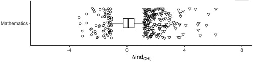
Generally, these 169 children are the positive outliers in Figure 1 and have large predicted differences in scores between kindergarten and third grade. The average difference between kindergarten and third grade for these children is 26 percentile points (SD = 11). For 127 children, their faster or slower growth rates change their score by at least one achievement level (> 20 percentile points) between kindergarten and third grade.

Discussion

The outline of this paper provides a framework that can be used to evaluate assumptions about the stability of early test scores. Since these assumptions define how we (i.e. researchers, teachers, parents, policy-makers) relate information of past and current test scores to future outcomes, it is vital that these assumptions are evaluated in a structured manner. By extending earlier work by Wohlwill (1973) and Tisak and Meredith (1990), this paper demonstrates the use of multilevel models in the evaluation of stability. As an illustration, we evaluated the assumption that function stability – examining a child’s individual growth curve in early standardized mathematics tests – provides additional information over linear stability – which assumes a persistent rank ordering of scores, in early mathematics test scores in the Netherlands.

The results showed that, although individual growth curves can provide significant supplementary information for some children, the gain in information is often small and differences over a short period are likely to be temporary inconsistencies rather than structural differences in growth. Although function stability had a significantly better fit than linear stability, linear stability is more likely for a large proportion of children. In addition, while some children did exhibit distinct growth rates, most of these differences are small and even extreme growth rates are only distinguishable from random fluctuations with relative certainty after five test administrations (i.e. 2.5 years). These results indicate that the test manual recommendation to use individual growth rates between subsequent measurements as a basis for identifying at-risk children will lead to a substantial amount of false-positive identifications.

This is exemplified by the number of score stagnations (i.e. no growth) that occur between kindergarten and third grade. Over 60% of the children in this sample show at least one stagnated score in this period. Teachers who consider individual growth in their decision to intervene are likely to overstate the significance of such stagnations. Furthermore, it is important to note that children tend to score markedly higher on the old version of the kindergarten mathematics test. A study by Keuning, Hilte, and Weekers (2014) have shown that tests from the LOVS are affected by norm inflation, which may provide an explanation for the differences between these test versions. This inflation may lead first-grade teachers to conclude that children who are tested with the old version of the kindergarten mathematics test drop in performance, when this drop is more likely a result of norm inflation.

As a method to evaluate stability, the MLM provides researchers with a flexible tool that can be used to test explicit assumptions about stability. In this paper, a selection of simple models was used to demonstrate their potential. However, these models can be extended to include situations that are far more complex. Although a more complex random-effect structure (second-order polynomial) was explored, this did not improve the model fit. The simple models provided a clear and practical interpretation in the light of existing test versions and test norms. Sensitivity to other factors, such as grade repetition, was explored but did not influence the conclusions.

Function stability and linear stability accord best with the recommendations of looking at the child’s score progression and score rank, respectively, and were selected for this reason. The assumption of strict stability was omitted in this study, as it is very unlikely that no growth in ability would have taken place between the test administration intervals. Furthermore, the necessary standardization that allows comparison of scores between kindergarten and later tests equalizes the first three models of strict, parallel and linear stability by setting the fixed time effects equal to zero. Other types of stability might be evaluated in contexts where such assumptions merit evaluation. For example, while strict stability is not an interesting or realistic assumption in the context of this study, the model for strict stability could be used to evaluate the assumption that personality or personal values remain stable over time. Such a model provides a simpler and more correct representation of the assumption being evaluated than the correlations and mean-change between two measurements that are commonly used (e.g. Asendorpf 1992; Vecchione et al. 2016)

The individual fit measure of $\mathrm{\Delta }\mathrm{i}\mathrm{n}{\mathrm{d}}_{\mathrm{C}\mathrm{H}{\mathrm{I}}_i}$ used in this study provides a sophisticated means of comparing the relative likelihood of competing models of stability for individuals and takes into account relative differences in structural (growth rate) and random (residual) fit. Unfortunately, this measure cannot be extended to suit a three-level model. To accommodate this drawback, a second model was estimated with school differences as a fixed effect. As school level intercepts were not our primary measure of interest and predictions for both approaches were closely aligned, the influence of this decision on the conclusions is presumably limited. A second limitation was the occurrence of missing data, which can lead to biased results and loss of power. When data are Missing At Random (MAR), multiple imputation provides an adequate way to deal with both problems (Graham 2009). It has the added benefit that the imputation model can be extended to include information that is not necessarily included in the model of interest but can be used to make predictions that are more accurate. In longitudinal data, the test scores available can be used to make accurate predictions about missing observations, as was made evident in this study by the low between-dataset variation.

Future research into stability should explicitly define the concept and use methods, such as those presented here, that accurately reflect this definition. In addition to the academic relevance of this framework, our findings may be especially important to teachers and parents involved in primary education who deal with these tests. Considering the large fluctuations relative to the small differences in individual growth curves, decisions based on individual growth rates in a few scores may easily lead to incorrect conclusions. Subsequent actions may result in either denying children much-needed care, based on falsely perceived progress, or providing additional care where none is needed. While our conclusions apply to the period between kindergarten and third grade, the fact that development tends to be more stable with age (Hartmann, Pelzel, and Abbott 2011) makes it likely that these results can be generalized to later ages. Additionally, although we described the development of scores over a four-year period, teachers may base decisions on far fewer test scores, which further increases the influence of random fluctuations. These findings underline the importance of a clear framework for evaluating existing assumptions about the stability of early development.

Disclosure statement

No potential conflict of interest was reported by the author(s).

Correction Statement

This article has been republished with minor changes. These changes do not impact the academic content of the article.

Notes

1 The terminology used by Tisak and Meredith is adopted throughout this paper. Strict, parallel, linear/monotonic and function stability are referred to by Wohlwill (1973, 362) as ‘absolute invariance’, ‘preservation of individual differences’, ‘consistency of relative position’ and ‘consistency relative to a prototypic function’, respectively. Similarly to Tisak and Meredith (1990), we did not consider two additional types (‘regularity of occurrence’ and ‘regularity of form of change’) as they do not refer to distinct types of linear models.

References

- Asendorpf, J. B. 1992. “Beyond Stability: Predicting Inter-Individual Differences in Intra-Individual Change.” European Journal of Personality 6 (2): 103–117. doi:10.1002/per.2410060204.
- Bates, D., M. Mächler, B. M. Bolker, and S. C. Walker. 2015. “Fitting Linear Mixed-Effects Models Using lme4.” Journal of Statistical Software 67 (1): 1–48. doi:10.18637/jss.v067.i01.
- Bornstein, M. H., E. Brown, and A. Slater. 1996. “Patterns of Stability and Continuity in Attention Across Early Infancy.” Journal of Reproductive and Infant Psychology 14 (3): 195–206. doi:10.1080/02646839608404517.
- Bornstein, M. H., C. Hahn, and O. M. Haynes. 2004. “Specific and General Language Performance Across Early Childhood: Stability and Gender Considerations.” First Language 24 (3): 267–304. doi:10.1177/0142723704045681.
- Bornstein, M. H., C. Hahn, D. L. Putnick, and J. T. D. Suwalsky. 2014. “Stability of Core Language Skill Stability of Core Language Skill from Early Childhood to Adolescence: A Latent Variable Approach.” Child Development 85 (4): 1346–1356. doi:10.1111/cdev.12192.
- Bornstein, M. H., and D. L. Putnick. 2012. “Stability of Language in Childhood: A Multiage, Multidomain, Multimeasure, and Multisource Study.” Developmental Psychology 48 (2): 477–491. doi:10.1037/a0025889.
- Bracken, B. A., and K. C. Walker. 1997. “The Utility of Intelligence Tests for Preschool Children.” In Contemporary Intellectual Assessment: Theories, Tests and Issues, edited by D. P. Flanaganm, J. L. Genshaft, and P. L. Harrison, 1st ed., 484–502. New York: The Guilford Press.
- COTAN. 2011. Toelichting bij de beoordeling Rekenen voor Kleuter Groep 1 en 2 LOVS Cito [Commentary on the Assessment of Mathematics for Preschoolers and Kindergarteners LOVS Cito]. Amsterdam: NIP.
- COTAN. 2013. Toelichting bij de beoordeling Taal voor Kleuters (TvK) [Commentary on the Assessment of Language for Preschoolers and Kindergarteners LOVS Cito]. Utrecht: NIP.
- Cronbach, L. J. 1971. “Test Validation.” In Educational Measurement, edited by R. L. Thorndike, 2nd ed., 443–507. Washington, DC: American Council on Education.
- Dockrell, J., A. Llaurado, J. Hurry, R. Cowan, and E. Flouri. 2017. Review of Assessment Measures in the Early Years: Language and Literacy, Numeracy, and Social Emotional Development and Mental Health. London: Institute of Education. doi:10.13140/RG.2.2.33853.97765.
- Duncan, G. J., C. J. Dowsett, A. Claessens, K. Magnuson, A. C. Huston, P. Klebanov, … C. Japel. 2007. “School Readiness and Later Achievement.” Developmental Psychology 43 (6): 1428–1446. doi:10.1037/0012-1649.43.6.1428.
- Gelderblom, G., K. Schildkamp, J. Pieters, and M. Ehren. 2016. “Data-Based Decision Making for Instructional Improvement in Primary Education.” International Journal of Educational Research 80: 1–14. doi:10.1016/j.ijer.2016.07.004.
- Graham, J. W. 2009. “Missing Data Analysis: Making It Work in the Real World.” Annual Review of Psychology 60: 549–576. doi:10.1146/annurev.psych.58.110405.085530.
- Hartmann, D. P., K. E. Pelzel, and C. B. Abbott. 2011. “Design, Measurement, and Analysis in Developmental Research.” In Developmental Science, an Advanced Textbook, edited by M. H. Bornstein, and M. E. Lamb, 6th ed., 109–198. New York: Psychology Press.
- Janssen, J., N. D. Verhelst, R. Engelen, and F. Scheltens. 2010. Wetenschappelijke verantwoording van de toetsen LOVS Rekenen-Wiskunde voor groep 3 tot en met 8 [Scientific Account of the LOVS Mathematics for First to Fifth Grade]. Arnhem: Cito.
- Kagan, J. 1971. Change and Continuity in Infancy. New York: John Wiley & Sons, Inc.
- Kagan, J. 1980. “Perspectives on Continuity.” In Constancy and Change in Human Development, edited by G. B. Orville, and J. Kagan, 26–74. London: Harvard University Press.
- Keuning, J., M. Hilte, and A. Weekers. 2014. “Begrijpend leesprestaties onderzocht - Een analyse op basis van Cito dataretour.” [Reading Comprehension Explored – An Analysis Based on Cito datareturn.] Tijdschrift Voor Orthopedagogiek 53: 2–13.
- Koerhuis, I., and J. Keuning. 2011. Wetenschappelijke verantwoording van de toetsen Rekenen voor kleuters [Scientific Account of the Mathematics for Preschoolers and Kindergartners Test]. Arnhem: Cito.
- La Paro, K. M., and R. C. Pianta. 2000. “Predicting Children’s Competence in the Early School Years: A Meta-Analytic Review.” Review of Educational Research 70 (4): 443–484. doi:10.3102/00346543070004443.
- Lerner, R. M., S. Lewin-Bizan, and A. E. Alberts Warren. 2011. “Concepts and Theories of Human Development.” In Developmental Science, an Advanced Textbook, edited by M. H. Bornstein, and M. E. Lamb, 6th ed., 3–50. New York: Psychology Press.
- Mashburn, A. J., and G. T. Henry. 2004. “Assessing School Readiness: Validity and Bias in Preschool and Kindergarten Teachers’ Ratings.” Educational Measurement: Issues and Practice 23 (4): 16–30. doi:10.1111/j.1745-3992.2004.tb00165.x.
- McCall, R. B. 1981. “Nature-Nurture and the Two Realms of Development: A Proposed Integration with Respect to Mental Development.” Child Development 52 (1): 1–12. doi:10.2307/1129210.
- Mroczek, D. K. 2007. “The Analysis of Longitudinal Data in Personality Research.” In Handbook of Research Methods in Personality Psychology, edited by R. W. Robins, R. C. Fraley, and R. F. Krueger, 543–556. New York: The Guilford Press.
- Nagle, R. J. 2000. “Issues in Preschool Assessment.” In The Psychoeducational Assessment of Preschool Children, edited by B. A. Bracken, 3rd ed., 19–32. Boston, MA: Allyn & Bacon.
- R Core Team. 2018. R: A Language and Environment for Statistical Computing. Vienna: R Foundation for Statistical Computing.
- Rubin, D. B. 1987. Multiple Imputation for Nonresponse in Surveys. New York: J. Wiley & Sons.
- Rudinger, G., and C. Rietz. 1998. “The Neglected Time Dimension? Introducing a Longitudinal Model Testing Latent Growth Curves, Stability, and Reliability as Time Bound Processes.” Methods of Psychological Research Online 3 (2): 109–130.
- Shepard, L. A. 1997. “The Centrality of Test Use and Consequences for Test Validity.” Educational Measurement: Issues and Practice 16 (2): 5–24. doi:10.1111/j.1745-3992.1997.tb00585.x.
- Singer, J. D., and J. B. Willett. 2003. Applied Longitudinal Data Analysis. New York: Oxford University Press.
- Snijders, T. A. B., and R. J. Bosker. 2012. Multilevel Analysis: An Introduction to Basic and Advanced Multilevel Modeling. 2nd ed. London: Sage Publications, Inc.
- Sterba, S. K., and J. Pek. 2012. “Individual Influence on Model Selection.” Psychological Methods 17 (4): 582–599. doi:10.1037/a0029253.
- Tisak, J., and W. Meredith. 1990. “Descriptive and Associative Developmental Models.” In Statistical Methods in Longitudinal Research 2, edited by A. Von Eye, 387–406. San Diego: Academic Press. http://ebookcentral.proquest.com.
- Van Buuren, S., and K. Groothuis-Oudshoorn. 2011. “MICE : Multivariate Imputation by Chained Equations in R.” Journal of Statistical Software 45 (3): 1–68.
- Vecchione, M., S. Schwartz, G. Alessandri, A. K. Döring, V. Castellani, and M. G. Caprara. 2016. “Stability and Change of Basic Personal Values in Early Adulthood: An 8-Year Longitudinal Study.” Journal of Research in Personality 63: 111–122. doi:10.1016/j.jrp.2016.06.002.
- Veldhuis, M., and M. Van den Heuvel-Panhuizen. 2014. “Primary School Teachers’ Assessment Profiles in Mathematics Education.” PLoS ONE 9 (1). doi:10.1371/journal.pone.0086817.
- Verhelst, N. D., C. A. W. Glas, and H. H. F. M. Verstralen. 1995. One-Parameter Logistic Model OPLM. Arnhem: Cito.
- Verhelst, N. D., H. H. F. M. Verstralen, and T. J. H. M. Eggen. 1991. Finding Starting Values for the Item Parameters and Suitable Discrimination Indices in the One-Parameter Logistic Model. Arnhem: Cito.
- Vlug, K. F. M. 1997. “Because Every Pupil Counts: The Success of the Pupil Monitoring System in The Netherlands.” Education and Information Technologies 2: 287–306. doi: 10.1023/A:1018629701040
- Wohlwill, J. F. 1973. The Study of Behavioral Development. New York: Academic Press.
- Wohlwill, J. F. 1980. “Cognitive Development in Childhood.” In Constancy and Change in Human Development, edited by G. B. Orville, and J. Kagan, 359–444. London: Harvard University Press.