Combining statistical and machine learning methods to explore German students’ attitudes towards ICT in PISA

ABSTRACT

In our age of big data and growing computational power, versatility in data analysis is important. This study presents a flexible way to combine statistics and machine learning for data analysis of a large-scale educational survey. The authors used statistical and machine learning methods to explore German students’ attitudes towards information and communication technology (ICT) in relation to mathematical and scientific literacy measured by the Programme for International Student Assessment (PISA) in 2015 and 2018. Implementations of the random forest (RF) algorithm were applied to impute missing data and to predict students’ proficiency levels in mathematics and science. Hierarchical linear models (HLM) were built to explore relationships between attitudes towards ICT and mathematical and scientific literacy with the focus on the nested structure of the data. ICT autonomy was an important variable in RF models, and associations between this attitude and literacy scores in HLM were significant and positive, while for other ICT attitudes the associations were negative (ICT in social interaction) or non-significant (ICT competence and ICT interest). The need for further research on ICT autonomy is discussed, and benefits of combining statistical and machine learning approaches are outlined.

KEYWORDS:

• Combining statistics and machine learning
• random forest
• multilevel modeling
• attitudes towards ICT
• ICT autonomy

Introduction

Educational researchers are facing a new challenge brought about by growing volumes of data. In order to cope with this challenge, creative adaptability of methods is required, which needs to be an integral part of academic training. Contemporary data science methodologies endeavour to integrate statistical analysis with the relatively novel machine learning approach, which aims at finding generalizable data patterns and making predictions on their basis (Breiman 2001b, Donoho 2017). In educational research, this integration remains to be attained: Machine learning is increasingly used for data analysis of large-scale educational surveys (Bethmann et al. 2014, Gabriel et al. 2018, Nationales Bildungspanel 2019, Saarela et al. 2016) but rarely in combination with statistical modeling. A flexible way to use statistical and machine learning methods can be advantageous for data analysis of a large-scale educational survey, as we illustrate with our analysis of German students’ attitudes towards information and communication technology (ICT).

Attitudes towards ICT, which have a considerable impact on learning (Fraillon et al. 2020, Organisation for Economic Co-operation and Development [OECD] 2015, 2019d), are examined in the frame of large-scale educational surveys (Eickelmann and Vennemann 2017, Fraillon et al. 2019). In this study, we used the ICT framework (Goldhammer et al. 2016) from the Programme for International Student Assessment (PISA). PISA is conducted by the OECD every three years, starting from 2000. It measures 15-year-old students’ literacy (competence required for coping with adult life) in different domains, attitudes to schooling, and a broad range of demographic factors. Literacy scores are translated into proficiency levels, from Level 1b to Level 6, using cut-off points (OECD 2017b); students with scores below the baseline Level 2 are classified as low performers and students with scores at Level 5 and above as high performers (OECD 2016b, 2019b, Pokropek et al. 2018).

Based on previous findings (Güzeller and Akin 2014, Luu and Freeman 2011, Petko et al. 2017, Zhang and Liu 2016), we explored students’ attitudes towards ICT in PISA 2015 and 2018 in relation to their mathematical and scientific literacy. We used solely German samples to avoid pitfalls outlined by critics of PISA with regard to international comparisons based on simplistic interpretations (Anderson et al. 2009, Goldstein 2004, Hopfenbeck et al. 2018, Zhao 2020). In order to determine the relative importance of attitudes towards ICT, we compared them with each other and with two demographic variables, which were shown to be influential factors for academic achievement in mathematics and science in Germany: economic, social and cultural status (ESCS) and gender (Mostafa and Schwabe 2019, OECD 2016a, 2019c, Rodrigues and Biagi 2017).

From the methodological perspective, our aim was to present a versatile way to apply statistical and machine learning methods to a large-scale educational survey. We selected the most suitable tools from statistical and machine learning toolboxes for each of the three consecutive tasks that we needed to complete. For the first task, missing data imputation, we chose random forest (RF), a machine learning algorithm (Stekhoven 2013). For the second task, predicting proficiency levels in mathematics and science (below Level 2, Levels 2–4, or Level 5 and above), another implementation of the RF algorithm (Breiman 2001a, Liaw and Wiener 2002) was used. For the third task, exploring associations between literacy scores and attitudes towards ICT with the focus on the hierarchical structure of the data, we resorted to a traditional statistical method, hierarchical linear modeling (HLM; Dedrick et al. 2009, Harrison et al. 2018, McCoach 2010). We justify our analytical decisions and discuss methodological recommendations for educational researchers interested in novel methods of data analysis.

In the second section of this paper, we describe the current state of research; in the third, we outline our analytical decisions; in the fourth, we report our results; and in the fifth, we discuss limitations of the study and its implications for future research. Our R script is freely available to the readers¹, to allow them to reproduce the findings of the study, practice data analysis with plausible values in a large-scale educational survey, or get acquainted with the basics of machine learning in R.

Theoretical background

In this section, we discuss statistical and machine learning methods in educational research and versatility in application of these approaches. Then we focus on the RF algorithm and model-agnostic methods, which make machine learning models interpretable. Finally, as we illustrate the use of these tools by exploring relationships between ICT attitudes and academic achievement in PISA 2015 and 2018, we briefly review previous research on this topic.

Statistical and machine learning methods in educational research

Statistical methods in educational research vary widely, and their comprehensive description is beyond the frame of this paper. In this study, we focus on multilevel methods, which are increasingly used for large-scale educational surveys (Anderson et al. 2009, OECD 2009), as failing to recognize the hierarchical structure of the data leads to Type I error inflation (Cheah 2009, Musca et al. 2011). Multilevel structural equation modeling (Areepattamannil and Santos 2019, Goldstein et al. 2007), multilevel latent class analysis (Yalçın 2018), multilevel multidimensional item response theory (Lu and Bolt 2015), and the most frequently used method, HLM (Areepattamannil 2014, Cosgrove and Cunningham 2011, Sun et al. 2012, Yıldırım 2012) were applied to hierarchical data in large-scale educational surveys. Methodological recommendations for the best practices in HLM were summarized by Dedrick et al. (2009) and Harrison et al. (2018).

In addition to statistical methods, the relatively novel machine learning approach has recently been applied to large-scale educational surveys (Bethmann et al. 2014, Gabriel et al. 2018, Nationales Bildungspanel 2019, Saarela et al. 2016). Shmueli (2010) discussed the contrast between explanatory modeling typical for statistics and predictive modeling in machine learning: ‘While statistical theory has focused on model estimation, inference and fit, machine learning and data mining have concentrated on developing computationally efficient predictive algorithms and tackling the bias-variance trade-off in order to achieve high predictive accuracy’ (p. 306). Machine learning differs from statistics in regard to data pre-processing (splitting the data into the training set and the test set), choice of variables (less theory-driven than in statistics), and model evaluation (predictive accuracy instead of explanatory power). Machine learning methods are widely used by such interdisciplinary communities as educational data mining and learning analytics (see Rienties, Køhler Simonsen, and Herodotou [2020], Romero and Ventura [2020]).

Integration of statistical and machine learning approaches has been discussed for more than two decades (Friedman 1997). Breiman (2001b) urged statisticians to embrace algorithmic thinking typical for machine learning. Hastie et al. (2009) presented a combination of statistical and machine learning methods to train the most effective predictive model for the dataset in question. Shmueli (2010) suggested a bi-dimensional approach that takes into consideration explanatory power and predictive accuracy of a model, thus combining statistical and machine learning approaches to model evaluation. Donoho (2017) stressed that data science, which uses scientific methods to create meaning from raw data, needs to include mutually enriching statistical and machine learning perspectives. In the frame of this integration, novel methods were developed which combine statistics and machine learning. For instance, Ryo and Rillig (2017) introduced statistically reinforced machine learning, in which machine learning models are augmented by investigating significance and effect sizes typical for statistical models. Another way to integrate statistics and machine learning is to exercise versatility in data analysis, when the researcher selects tools from either of these toolboxes depending on the study aims and the dataset characteristics (Breiman 2001b, Donoho 2017, Hastie et al. 2009). The best techniques for specific tasks can be chosen based on existing research on their comparative effectiveness (Breiman 2001b, Bzdok et al. 2018, Couronné et al. 2018, Makridakis et al. 2018).

In educational science, however, integration of statistics and machine learning remains to be attained. We demonstrate that the two approaches can be combined for data analysis of a large-scale educational survey, and it would be beneficial for statisticians to widen the scope of their techniques with machine learning methods. One of these methods, RF, is discussed in detail in the next section.

Random forest and model-agnostic methods

RF, which has recently grown from a single algorithm (Breiman 2001a) into a framework of various models (Denil et al. 2014, Fawagreh et al. 2014), is increasingly used in educational research (Beaulac and Rosenthal 2019, Golino et al. 2014, Han et al. 2019, Hardman et al. 2013, McDaniel 2018, Spoon et al. 2016, Yi and Na 2019). RF belongs to the family of algorithms based on decision trees. The idea of a decision tree is to split the dataset on a particular variable based on information gained from this split. As splits are binary (yes or no), continuous variables are transformed into categorical variables, that is, lesser than or greater than a certain value. Figure 1 shows a decision tree predicting students’ mathematical proficiency (the classification task), which we built for illustration purpose. For this decision tree, the first two splits are based on the ESCS value, and the third on the value of ICT autonomy.

Figure 1. Decision Tree for Mathematical Proficiency Levels in PISA 2015. Note: Split labels specify how the decision tree splits the data. Node labels contain the following information: the predicted class for the node; the probability per class of observations in the node (conditioned on the node, the sum across a node is 1); and the percentage of observations in the node. ESCS = economic, social, and cultural status; AUTO = ICT autonomy; INTE = ICT interest; SOCI = ICT in social interaction; class 1 = mathematical proficiency below Level 2; class 2 = Levels 2–4; class 3 = Level 5 and above.

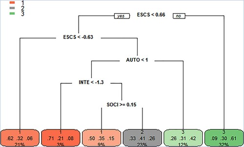
Decision trees have a number of advantages: They are interpretable as they mirror human decision-making more than other predictive models, they handle a wide range of problems and different types of variables, and they impose no assumptions on the data (Golino and Gomes 2014). Their substantial disadvantage is the problem of overfitting, when the algorithm performs poorly in new datasets. This problem is resolved in RF by generating a large number of bootstrapped trees based on random samples of variables (a ‘forest’ of decision trees) and aggregating their results.

RF is effective for highly dimensional data and handles interactions and nonlinearity (Fawagreh et al. 2014, Molnar 2019). It has become a widely used method for classification tasks (Denil et al. 2014), as it has lower predictive error than logistic regression (Breiman 2001b, Couronné et al. 2018), and for multiclass tasks, it does not require the proportional odds assumption needed for ordinal regression (Field et al. 2017, O’Connell and Liu 2011). RF is increasingly used for missing data imputation, as it is adaptive to interactions and nonlinearity (Shah et al. 2014), performs well even with data missing not at random (Tang and Ishwaran 2017), and has better imputation accuracy than nearest neighbours imputation and multiple imputation by chained equations (Misztal 2019, Waljee et al. 2013). Therefore, Golino and Gomes (2016) suggested using RF to impute missing data in educational and psychological research.

To measure model performance of RF, different metrics can be used (Chai and Draxler 2014, Janitza et al. 2014). One of the most commonly used metrics is the area under the Receiver Operating Characteristic (ROC) curve (Kleiman and Page 2019). ROC is a probability curve, which is plotted with true positive rate on the y-axis against false positive rate on the x-axis. The area under the curve (AUC) represents the ability of the model to separate classes. For a perfect classifier, the area is 100%, and for a random classifier, when true positive rate is equal to false positive rate, it is 50%. AUC can be extended to multiclass problems, with separate comparisons for each pair of classes (Hand and Till 2001).

RF models are better predictors than decision trees, but they are less understandable. Breiman (2001b) described this trade-off between accuracy and interpretability of a model as the Occam dilemma. In order to make the output of such ‘black boxes’ more understandable, model-agnostic (that is, flexibly applicable to any model) methods can be used, such as permutation variable importance and partial dependence plots (Molnar 2019).

The concept of permutation variable importance can be briefly explained as follows. A variable is ‘considered important if deleting it seriously affects prediction accuracy’ of the model (Breiman 2001b, p. 230). However, removing one variable after another and retraining the model each time would be computationally expensive, and instead of it, we replace a variable with random noise to see how it influences the model’s performance. The noise is created by permuting the variable (that is, shuffling its values). Permutation variable importance was shown to be less biased than other variable importance measures (Altmann et al. 2010).

Partial dependence plot for a variable shows the marginal effect that it has on the predicted outcome of the model (Molnar 2019). It depicts the nature of the relationship between the variable and the outcome and indicates whether this relationship is linear, monotonic etc. In classification tasks, partial dependence plots can be built for each class separately to show the probability for the class given the values of the variable. Partial dependence plots can be constructed for two variables in 3D to display not only their influence on the outcome but also their interactions with each other (Greenwell 2017).

Based on the findings showing effectiveness of RF for missing data imputation and for classification tasks, we chose the RF algorithm for these tasks in our study. Model-agnostic methods (variable importance and partial dependence plots) were used to increase interpretability of the models.

Attitudes towards ICT in PISA

Attitude is a multifaceted structure comprised of affective, cognitive, and behavioural components (Guillén-Gámez and Mayorga-Fernández 2020). Attitudes towards ICT were conceptualized in different ways (Zhang, Aikman, and Sun 2008) and examined in the frame of large-scale educational surveys (Eickelmann and Vennemann 2017, Fraillon et al. 2019, Fraillon et al. 2020). In the current study, the ICT framework from PISA 2015 (Goldhammer et al. 2016) was used.

In previous PISA waves, the ICT framework was different: PISA 2003, 2006, and 2009 assessed students’ confidence related to the three types of ICT tasks (basic, Internet-related, and high-level tasks). In PISA 2012, positive components of attitude towards ICT (perceiving ICT as a useful tool) were measured as a construct independent from negative components (perceiving ICT as an uncontrollable entity). As ICT literacy measure has not been developed in PISA yet, attitudes towards ICT were studied in relation to mathematical and scientific literacy. In PISA 2003–2012, positive attitudes towards ICT were significantly and positively associated with mathematical and scientific literacy scores (Güzeller and Akin 2014, Luu and Freeman 2011, Petko et al. 2017, Zhang and Liu 2016).

In PISA 2015, the new conceptualization of ICT engagement (Goldhammer et al. 2016) was introduced. This framework was based on self-determination theory (Deci and Ryan 2000) and included dimensions of ICT competence, ICT interest, ICT autonomy, and ICT in social interaction (see Appendix A). Scale indices for each dimension were obtained in the frame of item response theory by means of generalized partial credit model, which allowed for the item discrimination to vary between items within any given scale (OECD 2017b). It was shown (Kunina-Habenicht and Goldhammer 2020, Meng et al. 2019) that the scales were reliable instruments with expected dimensionality. The same ICT framework was used in PISA 2018.

Recent findings on attitudes towards ICT in PISA 2015 showed that ICT autonomy was significantly positively associated with mathematical and scientific literacy scores in all countries participating in the optional questionnaire (Hu et al. 2018), and ICT in social interaction was significantly negatively associated with these scores in all countries (Hu et al. 2018). For ICT competence and ICT interest, the significance and the sign of their relationships with literacy scores varied at the country-specific level (Hu et al. 2018, Meng, Qiu, and Boyd-Wilson 2019, Odell et al. 2020).

In the current study, we re-examined the associations between German students’ attitudes towards ICT and mathematical and scientific literacy in PISA 2015 using a different methodology than Meng et al. (2019); additionally, we explored these associations in PISA 2018. We also used attitudes towards ICT to predict students’ proficiency in mathematics and science (below Level 2, Levels 2–4, or Level 5 and above) in PISA 2015 and PISA 2018.

Methods

Dataset

The data for the study was obtained from the OECD website, PISA 2015 and 2018 databases (OECD n.d.-a, n.d.-b).² The authors used German subsets of PISA student questionnaire and the optional ICT familiarity questionnaire for students. Cases with 100% missing ICT responses, which were due to the fact that the ICT questionnaire was optional in Germany, were removed (Reiss et al. 2016). In accordance with this criterion, 1093 cases (16.81%) were removed from the 2015 dataset and 944 cases (17.32%) were removed from the 2018 dataset before the analysis. The resulting 2015 sample consisted of 5411 students (50.71% female, n = 2744; 49.29% male, n = 2667) from 254 German schools. The resulting 2018 sample consisted of 4507 students (47.33% female, n = 2133; 52.67% male, n = 2374) from 208 German schools.

Measures

Mathematical and scientific literacy

Mathematical literacy is defined as ‘an individual’s capacity to formulate, employ and interpret mathematics in a variety of contexts’ (OECD 2017a, p. 67). Scientific literacy is defined as ‘the ability to engage with science-related issues, and with the ideas of science, as a reflective citizen’ (OECD 2017a, p. 22). Ten plausible values were included in analysis for each literacy score (OECD 2009). In both PISA waves, the cut-off score for performance below Level 2 in mathematics was 420.07 and in science 409.54. The cut-off score for performance at Level 5 and above in mathematics was 606.99 and in science 633.33 (OECD 2019b).

Demographics

ESCS is a composite score based on the three indicators: parental education, highest parental occupation, and home possessions. The latter indicator is used in PISA as a proxy for family wealth (OECD 2017a). The measure is constructed via principal component analysis and standardized for a standard deviation of one, with zero representing the overall OECD average (OECD 2017a). In the datasets, gender was coded as 1 for female and 2 for male. We recoded it as 0 for female and 1 for male.

Attitudes towards ICT

Attitudes towards ICT were measured with the 4-point Likert scale from strongly disagree to strongly agree, and the following IRT-scaled indices were calculated (OECD 2017b): (a) perceived ICT competence (COMPICT) on five items of the IC014 scale; (b) interest to ICT (INTICT) on six items of the IC013 scale; (c) ICT in social interaction (SOIAICT) on five items of the IC016 scale; and (d) ICT autonomy (AUTICT) on five items of the IC015 scale. The measures were the same in PISA 2018 (OECD 2019a).

Analytical strategy

In this section, we describe our analytical choices in completing the three consecutive tasks: (a) missing data imputation; (b) the classification task with proficiency levels (below Level 2, Levels 2–4, or Level 5 and above) as the categorical outcome variable, and (c) the regression task with the literacy score as the continuous outcome variable. The data were analysed with R, version 4.0.0 (R Core Team 2018). The R script is available at https://github.com/OlgaLezhnina/PISAstatsML and in Supplemental Materials.

Missingness patterns were checked with the package VIM (Kowarik and Templ 2016). For missing data imputation, we used the RF algorithm as an effective and unbiased method (Golino and Gomes 2016, Misztal 2019, Waljee et al. 2013) and chose the package missForest (Stekhoven 2013), as this implementation was shown to be more robust than other versions of RF imputation (Tang and Ishwaran 2017). Histograms of variables for the complete cases and the dataset after imputation were compared to visually assess the results of imputation. The imputed data were used for further analysis.

For predicting students’ proficiency levels in mathematics and science (below Level 2, Levels 2–4, or Level 5 and above), RF classification models were built, and attitudes towards ICT, ESCS and gender were used as predictors. We preferred RF to ordinal regression, as it does not require proportional odds assumption (O’Connell and Liu 2011) and handles nonlinearity and interactions (Fawagreh et al. 2014, Molnar 2019). We used the package randomForest (Liaw and Wiener 2002), which is a simple and commonly used implementation of the algorithm based on Breiman’s (2001a) original code. As the sample was imbalanced (there were substantially more students on Levels 2–4), we oversampled the training set with the package UBL (Branco et al. 2016). To avoid excessively optimistic performance assessment, we evaluated the models on the test set (20% of the 2015 data) which was not oversampled; and then, on the 2018 data. AUC was used as a measure of model performance; multiclass AUC and separate class comparisons were estimated with the package pROC (Robin et al. 2011). The mean decrease in accuracy (permutation importance) was chosen as a variable importance measure. Partial dependence plots for each predictor were built with the package pdp (Greenwell 2017). Three-dimensional partial dependence plots for pairs of predictors were built to illustrate their relationships with each other and with the predicted outcome.

In order to obtain a more detailed picture of relationships between attitudes towards ICT and mathematical and scientific literacy with the focus on the nested structure of the data (different schools), we needed a multilevel regression model. Our RF models were not hierarchical due to a limit for factor levels in randomForest (Liaw and Wiener 2002), and we had to choose a different method to build such a model. It was shown that for predictive multilevel models (such as RF), an increase in group size is more beneficial than an increase in the number of groups, while for estimative models (such as HLM) the opposite is the case (Afshartous and de Leeuw 2005). The group size in our case was the number of student participants in each school, and the number of groups was the number of schools. In both datasets, the group size varied from one to 30 students, while the number of groups was rather large (254 for the 2015 dataset and 208 for the 2018 dataset), which made HLM our instrument of choice.

HLM was conducted with the package lme4 (Bates et al. 2015) in accordance with methodological recommendations summarized by Dedrick et al. (2009) and Harrison et al. (2018). Restricted maximum likelihood was used as an estimation method (Dedrick et al. 2009). Independent variables were grand-mean centred and standardized by two standard deviations for comparability of continuous and binary variables (Gelman 2008). The need for multilevel modeling was assessed by exploring variance decomposition in null (unconditional) models with random intercepts (McCoach 2010). As full models with random slopes and random intercepts (Harrison et al. 2018) failed to converge, full models with random intercepts were built. To estimate sampling variance, Fay's method with 80 replicates was used, and statistical estimates were averaged for 10 plausible values (OECD 2009). Formulae for analysis with plausible values and replicate weights, which we used in our R script, are given in Appendix B. As we had only six predictors (gender, ESCS and four ICT attitudes), they were all included in the model simultaneously (see Heinze et al. [2018] for variable selection methods). Significance of estimates was assessed with the type III Wald test (Luke 2017), and a significance level of .001 was set as appropriate for our procedures and for the sample size (Lakens et al. 2018). Nakagawa’s marginal and conditional R² (Nakagawa and Schielzeth 2013, Nakagawa et al. 2017) were calculated with the package performance (Lüdecke et al. 2020). Assumptions for residuals were checked with diagnostic plots from the package sjPlot (Lüdecke 2019). In check for multicollinearity, the cut-off value of 3 for the variance inflation factor was used as recommended by Zuur et al. (2010). Intra-class correlation coefficients (ICCs) and Nakagawa’s marginal and conditional R² were reported as effect size measures for random effects (LaHuis et al. 2014, Lorah 2018).

Results

Random Forest for missing data imputation and classification tasks

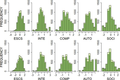
In the 2015 dataset, 2.41% of the data was missing, and 3.81% of the data was missing in the 2018 dataset. Aggregation plots and scatter matrices for missing values (see the R script) suggested that the data was missing at random, as there were no discernible patterns in missingness. RF imputation was conducted with the default settings (the number of trees = 100, the maximal number of iterations = 10). Histograms of variables from the complete cases dataset and the dataset after imputation (see Figure 2) showed that the imputation did not lead to changes in their distributions that could potentially bias our models.

Figure 2. Histograms of Complete Cases and Imputed Data in Years 2015 and 2018.Note: The upper row is for the 2015 data, the lower row for the 2018 data. Dark green = complete cases, light green = imputed data. ESCS = economic, social, and cultural status; INTE = ICT interest; COMP = ICT competence; AUTO = ICT autonomy; SOCI = ICT in social interaction.

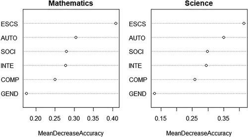
To predict students’ proficiency levels (below Level 2, Levels 2–4, or Level 5 and above), two RF models were trained: the mathematics model and the science model. The training set (80% of the 2015 dataset) was used. Variable importance plots for the models are shown in Figure 3. Attitudes towards ICT were less important than ESCS but more important than gender in both models, and ICT autonomy was more important than other attitudes.

Figure 3. Permutation Variable Importance. Note: ESCS = economic, social, and cultural status; AUTO = ICT autonomy; SOCI = ICT in social interaction; INTE = ICT interest; COMP = ICT competence; GEND = gender.

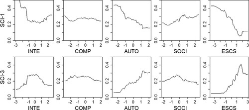
Variable importance measures do not indicate whether association of a variable with the predicted outcome is positive or negative; this information can be obtained from partial dependence plots for each variable. In Figure 4, the partial dependence plots for the science model are shown, and the plots for the mathematics model (see the R script) revealed similar patterns. In the upper row, we see the probability for a student to perform below Level 2, and in the lower row, the probability to perform on Level 5 and above, as predicted by ICT interest, ICT competence, ICT autonomy, ICT in social interaction, and ESCS. In the plots, higher levels of ICT autonomy predicted a higher probability for a student to perform on Level 5 and above in science, while lower levels of autonomy increased a probability to perform below Level 2. For ICT in social interaction, the partial dependence plots gave the opposite picture: higher levels of this attitude predicted a higher probability to perform below Level 2. The plots show nonlinearity of relationships between predictors and the predicted outcome, which is most clearly seen for ICT interest.

Figure 4. Partial Dependence Plots for Variables in the Science Model. Note: INTE = ICT interest; COMP = ICT competence; AUTO = ICT autonomy; SOCI = ICT in social interaction; ESCS = economic, social, and cultural status; SCI-1 = probability for class 1 (below Level 2); SCI-3 = probability for class 3 (Level 5 and above).

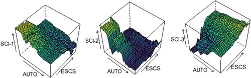
Partial dependence plots for pairs of variables indicated nonlinear relationships between them in terms of probability of the predicted outcome for each class (below Level 2, Levels 2–4, or Level 5 and above). In Figure 5, partial dependence plots for ESCS and ICT autonomy, the two most important variables, are shown for the science model. It can be seen that the highest probability for a student to perform on Level 5 and above in science was predicted by high levels in both ESCS and ICT autonomy.

Figure 5. Partial Dependence Plots for ESCS and ICT Autonomy in the Science Model.Note: ESCS = economic, social, and cultural status; AUTO = ICT autonomy; SCI-1 = probability for class 1 (below Level 2); SCI-2 = probability for class 2 (Levels 2–4); SCI-3 = probability for class 3 (Level 5 and above).

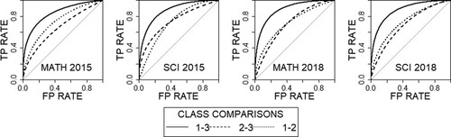
The models were evaluated on the test set from the 2015 data (20% of the sample). The multiclass AUC was 67.44% for the mathematics model and 71.66% for the science model. When evaluated on the 2018 data (the whole dataset), the multiclass AUC was 69.19% for the mathematics model and 68.51% for the science model. Although the model performance was suboptimal (see Limitations section), it is noteworthy that it did not change considerably for the 2018 data. The ROC curves for the class comparisons are presented in Figure 6.

Figure 6. Receiver Operating Characteristic Curves for the Models Evaluated on the 2015 Test Set and the 2018 Data. Note: SCI = Science; MATH = Mathematics; TP = True Positive; FP = False Positive; class 1 = proficiency below Level 2; class 2 = Levels 2–4; class 3 = Level 5 and above.

Multilevel modeling

Unconditional models for mathematical literacy and scientific literacy were built. For mathematical and scientific literacy, multilevel modeling was required, as can be seen from ICC values reported in Table 1.

Table 1. Unconditional Models for Mathematical Literacy and Scientific Literacy.

	Mathematical Literacy		Scientific Literacy
	2015	2018	2015	2018
Fixed effects
Intercept	506.35*** (1.86)	503.76***(1.07)	510.87*** (1.24)	506.22***(1.07)
Random effects
Intercept var.	3636.65	3822.62	4428.87	4628.37
Residual var.	4541.25	5162.91	5457.53	5956.34
Effect size
ICC	.445	.425	.448	.437

Note: In the 2015 dataset, N = 5411; in the 2018 dataset, N = 4507. Standard errors are in parentheses. Fixed effects are parameter estimates. Random effects are variance estimates. ICC = intraclass correlation coefficient.

*** p < .001.

For mathematical literacy and scientific literacy, full models with random intercepts were built. Fixed and random effects estimates are reported in Table 2.

Table 2. Full Models for Mathematical Literacy and Scientific Literacy.

	Mathematical Literacy		Scientific Literacy
	2015	2018	2015	2018
Fixed effects
Intercept	496.16***(1.83)	495.08***(2.08)	505.61***(1.69)	501.20***(1.99)
Gender	22.77*** (2.92)	18.99*** (3.04)	13.78*** (2.26)	12.57*** (3.02)
ESCS	24.59*** (3.00)	33.03*** (3.72)	30.12*** (2.71)	35.97*** (3.62)
Competence	−6.04 (3.63)	−3.15 (3.66)	−6.48 (3.08)	−2.75 (3.84)
Interest	0.15 (3.16)	2.01 (3.11)	−3.63 (2.55)	−0.47 (3.34)
Social interaction	−10.76*** (2.88)	−9.21*** (3.18)	−14.33*** (2.88)	−21.08*** (3.25)
Autonomy	22.56*** (3.28)	17.45*** (3.41)	38.29*** (2.88)	25.99*** (3.83)
Random effects
Intercept var.	2948.67	2897.46	3402.02	3377.05
Residual var.	4218.22	4859.19	5009.35	5614.08
Effect size
R², marginal	.055	.055	.066	.057
R², conditional	.444	.408	.444	.411

Note: In the 2015 dataset, N = 5411; in the 2018 dataset, N = 4507. Standard errors are in parentheses. Fixed effects are parameter estimates. Random effects are variance estimates. Effect size is Nakagawa’s R². ESCS = economic, social, and cultural status. Gender was recoded as 0 = female and 1 = male. In the 2018 dataset, the relationship between mathematical literacy and ICT in social interaction was nonsignificant at level .001 in three out of 10 models.

*** p < .001.

Assumptions for the full models were checked for each of 10 plausible values in mathematical and scientific literacy in the 2015 dataset and the 2018 dataset. Values of the variance inflation factor were below the cut-off value of 3, indicating that there was no multicollinearity in the data. Diagnostic plots for residuals showed that linearity and homoscedasticity assumptions were met, and residuals of the models were normally distributed.

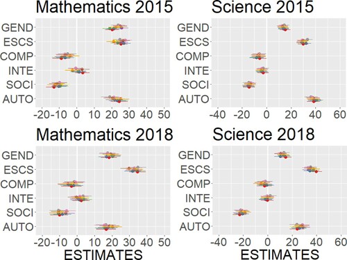
As the data was standardized by two standard deviations, we could compare the relative importance of all variables, including binary (gender), based on their regression coefficients. ICT in social interaction was significantly negatively associated with mathematical literacy and scientific literacy. ICT autonomy was significantly positively associated with mathematical literacy and scientific literacy, and it was almost as influential as gender and ESCS for mathematical literacy both in the 2015 dataset and in the 2018 dataset. Its association with scientific literacy (β = 38.29) was the strongest among all variables in the 2015 dataset and the second strongest after ESCS in the 2018 dataset (β = 25.99). In Figure 7, regression coefficients of all variables are shown with confidence intervals in different colours for 10 plausible values.

Figure 7. HLM Estimates for 10 Plausible Values with Confidence Intervals. Note: GEND = gender; ESCS = economic, social, and cultural status; COMP = ICT competence; INTE = ICT interest; SOCI = ICT in social interaction; AUTO = ICT autonomy.

Discussion

Findings on attitudes towards ICT

The findings of the study, which are consistent with previous studies (Hu et al. 2018, Meng et al. 2019), show that ICT in social interaction was significantly negatively associated with mathematical and scientific literacy, while ICT competence, the least important attitudinal variable in RF models, was not significantly associated with literacy scores in HLM. Negative associations of German students’ mathematical and scientific literacy with ICT interest in PISA 2015 were reported as significant by Meng et al. (2019) but were non-significant in our study. This discordance that can be explained by the difference in analytical choices, which are to some degree inevitably subjective and need to be reported transparently, so that they can be tested in further research (see Silberzahn et al. [2018]).

Our results on ICT autonomy, which are also congruent with previous studies (Hu et al. 2018, Meng et al. 2019), suggest that this attitude might play a prominent role in mathematics and science domains. For German students, ICT autonomy was an important variable in classification models, and it was significantly positively associated with literacy scores in HLM in PISA 2015 and PISA 2018. The role of ICT autonomy is probably not fully recognized by contemporary educational systems, with their emphasis on collaborative learning and group activities (Dillenbourg et al. 2009). In line with this tendency, the OECD focuses increasingly on collaborative problem solving in PISA, with less attention paid to learners’ autonomy. The change in the optional ICT questionnaire planned for PISA 2021 (Lorenceau et al. 2019) is indicative of this trend, as it seems that ICT autonomy in its current operationalization will cease to be a topic of research in PISA (OECD 2019d). We strongly believe, however, that research on ICT autonomy and its development in students (Areepattamannil and Santos 2019) are crucially important for the educational system. In our contemporary world, which requires ability to make independent decisions and interact with increasingly digitalized environment, ICT autonomy might become one of the main building blocks of effective learning.

Combining statistical and machine learning approaches to data analysis

In the current study, we presented a flexible way to combine statistical and machine learning methods for data analysis of a large-scale educational survey. For each task in the analytical process, we chose the most suitable tool from either statistical or machine learning toolbox and justified our analytical decisions.

As missing data is a persistent problem in PISA (Hopfenbeck et al. 2018) and in large-scale educational surveys in general (Golino and Gomes 2016), educational researchers need to keep themselves informed about different statistical and machine learning imputation techniques. For this task, we chose the RF algorithm implemented in the package missForest based on previous studies showing its effectiveness (Misztal 2019, Waljee et al. 2013) and checked the quality of imputation with histograms of the imputed data in comparison to the complete cases. We would suggest that researchers include RF imputation in their toolbox as an effective and unbiased imputation method.

With a different RF implementation from the package randomForest, we built classification models for scientific and mathematical proficiency levels of German students in PISA 2015 and PISA 2018. We adhered to the three-part division of proficiency levels (below Level 2, Levels 2–4, or Level 5 and above) accepted in PISA (OECD 2016b, 2019b, Pokropek et al. 2018), but another classification task, such as predicting the whole range of proficiency levels or low vs regular academic performance (a binary task), would be also possible. While choosing an instrument for this task, we preferred RF to ordinal regression (O’Connell and Liu 2011) and to more sophisticated machine learning models (see Limitations section). A different analytical decision for the same dataset is also feasible (Silberzahn et al. 2018). Performance of the models built for the 2015 data did not decrease on the 2018 data, indicating that the same patterns persisted in both years. With the help of model-agnostic methods (variable importance and partial dependence plots), we assessed the relative importance of our variables (attitudes towards ICT, ESCS, and gender) for proficiency levels and visually presented relationships between the predictors and the predicted outcome. Thus, we observed nonlinear relationships between the predictors as indicated by the partial dependence plots. We recommend using model-agnostic methods in educational research to increase interpretability of machine learning models.

As we learnt from the RF models that students’ ICT attitudes were important for predicting their proficiency levels, we decided to explore relationships between these variables and mathematical and scientific literacy in more detail. The data had a hierarchical structure; in our choice of an instrument for multilevel modeling, we relied on previous studies indicating that in our case, HLM was preferable to machine learning models because of the dataset characteristics (Afshartous and de Leeuw 2005). With HLM, we obtained information on fixed and random effects, such as significance of relationships, their direction, and effect sizes. The 2018 data revealed the same patterns in associations between ICT attitudes and literacy scores as the 2015 data, and fixed effects estimates in HLM for these two years did not substantially differ.

Combining machine learning and statistical approaches is beneficial for research on large-scale educational surveys, as the former is a valuable tool for finding generalizable patterns, while the latter is useful for testing hypotheses and making statistical inferences. A flexible choice of analytic instruments from both toolboxes depending on the study aims and the dataset characteristics is an effective way of analysing the data.

Limitations and further research

The limitations of the study are related to PISA design and to our goals, which determined our analytical choices. We briefly outline both areas of limitations.

As any cross-sectional design, PISA cannot allow us to establish causal relationships but only to detect associations between variables; the question of causality should be left to longitudinal or experimental studies. The following flaws of PISA sampling design were mentioned in literature and summarized by Hopfenbeck et al. (2018) and Zhao (2020): (a) exclusion of students with disabilities from PISA is problematic, as it prevents them from taking part in policy aiming at educational equity (Schuelka 2013); (b) there is a sampling bias towards slower-maturing students, as some students are excluded because of early graduation, dropout or other forms of attrition (Anderson et al. 2009); and (c) age criterion for selecting participants means that students might have had different exposure to curriculum, as some of them might have repeated a class or skipped one (Prais 2004). Concerns have been raised about plausible values in PISA, which are constructed even for students who have not taken a single item on the subject (Kreiner and Christensen 2014). In addition, in attitudes towards ICT, as in any self-report measures, social desirability might be a source of bias.

In this study, we chose simple and commonly used implementations of RF to make our analytical procedures more understandable and our R script easily reproducible. A more sophisticated implementation of the algorithm for the classification task (Janitza et al. 2014, Ryo and Rillig 2017, Strobl et al. 2007) with model hyperparameters tuned with the package mlr (Schiffner et al. 2016) would have probably led to a better model performance. Another limitation, which is relevant both to RF and HLM models, is determined by our choice of variables. Both HLM and RF models would have benefited from adding more variables related to these domains, such as science attitudes in PISA 2015 (Areepattamannil and Santos 2019); the RF algorithm could have effectively selected the most relevant variables out of a wider scope of attitudinal and demographic factors. Exploring the whole range of factors that influence mathematical and scientific literacy was not, however, the goal of this study. We intended to use the same variables in all our models, so that attitudes towards ICT could be compared with each other and with ESCS and gender; for HLM, the nested structure of the data (different schools) was also taken into account. The other reason for not including more variables, as well as another limitation of the study, was related to the issue of model convergence. HLM with random intercepts and slopes (Harrison et al. 2018) failed to converge, and we had to resort to random intercept models. In further research, more advanced statistical and machine learning methodology can be applied (Romero and Ventura 2020, Ryo and Rillig 2017).

Conclusion

In this study, statistical and machine learning models were used to explore German students’ attitudes towards ICT in PISA 2015 and PISA 2018. We demonstrated the benefits of choosing the most suitable methods from statistical and machine learning toolboxes for data analysis of a large-scale educational survey. For the first task, missing data imputation, and the second, predicting proficiency levels, we used the RF algorithm, while for the third task, exploring associations between literacy scores and attitudes, we resorted to HLM. Findings obtained with our classification models (RF) and regression models (HLM) indicate that ICT autonomy might play a prominent role in mathematics and science domains and needs to be studied further. The flexible way to combine statistical and machine learning approaches can be recommended to educational researchers, as in our age of growing data volumes and complexity, creative adaptability and versatility are indispensable. As Breiman (2001b, p. 204) said, ‘To solve a wider range of data problems, a larger set of tools is needed’.

Acknowledgements

We are grateful to Manuel Prinz for his insightful comments on the first draft, to Junaid Ghauri for thought-provoking discussions, and to anonymous reviewers for their criticism and constructive suggestions that helped us substantially improve the manuscript.

Disclosure statement

No potential conflict of interest was reported by the author(s).

Notes

1 See the R script in Supplemental Materials or at https://github.com/OlgaLezhnina/PISAstatsML

2 The PISA database, see http://www.oecd.org/pisa/data/2015database/ and http://www.oecd.org/pisa/data/2018database/.

Appendices

Appendix A. The ICT engagement framework

IC013: ICT Interest

IC013Q01NA. I forget about time when I'm using digital devices.

IC013Q04NA. The Internet is a great resource for obtaining information I am interested in (e.g. news, sports, dictionary).

IC013Q05NA. It is very useful to have social networks on the Internet.

IC013Q11NA. I am really excited discovering new digital devices or applications.

IC013Q12NA. I really feel bad if no internet connection is possible.

IC013Q13NA. I like using digital devices.

IC014: ICT Competence

IC014Q03NA. I feel comfortable using digital devices that I am less familiar with.

IC014Q04NA. If my friends and relatives want to buy new digital devices or applications, I can give them advice.

IC014Q06NA. I feel comfortable using my digital devices at home.

IC014Q08NA. When I come across problems with digital devices, I think I can solve them.

IC014Q09NA. If my friends and relatives have a problem with digital devices, I can help them.

IC014: ICT Autonomy

IC015Q02NA. If I need new software, I install it by myself.

IC015Q03NA. I read information about digital devices to be independent.

IC015Q05NA. I use digital devices as I want to use them.

IC015Q07NA. If I have a problem with digital devices I start to solve it on my own.

IC015Q09NA. If I need a new application, I choose it by myself.

IC014: ICT in Social Interaction

IC016Q01NA. To learn something new about digital devices, I like to talk about them with my friends.

IC016Q02NA. I like to exchange solutions to problems with digital devices with others on the internet.

IC016Q04NA. I like to meet friends and play computer and video games with them.

IC016Q05NA. I like to share information about digital devices with my friends.

IC016Q07NA. I learn a lot about digital media by discussing with my friends and relatives.

Appendix B. Formulae for analysis with plausible values and replicate weights

Instructions given by PISA Data Analysis Manual (OECD 2009) on computation of statistical estimates and standard errors with plausible values and replicate weights can be summarized as follows:

1. To calculate a final estimate (e.g. a regression coefficient), estimates for models with all plausible values and the final weight are averaged (OECD 2009, p. 118): $\theta ={\displaystyle \frac{1}{M}\sum _{i=1}^M{\theta }_{\mathrm{i}}}$

2. The standard error of this final estimate is calculated as follows:

   • (2.1) The sampling variance is calculated by averaging sampling variances for all plausible values (OECD 2009, p. 118): ${\sigma }^2={\displaystyle \frac{1}{M}\sum _{i=1}^M{\sigma }_{\mathrm{i}}^2}$

   • Each of them is calculated as the averaged (with the coefficient specified below) sum of squared differences between the final estimate and each of replicate estimates (OECD 2009, pp. 73–74): ${\sigma }_{\mathrm{i}}^2={\displaystyle \frac{1}{G(1-k{)}^2}\sum _{i=1}^G({\theta }_{\mathrm{i}}-\theta {)}^2}$

   • (2.2) The imputation variance is calculated as the averaged (with the coefficient specified below) sum of squared differences between the final estimate and an estimate for each of plausible values (OECD 2009, p. 100): $B={\displaystyle \frac{1}{M-1}\sum _{i=1}^M({\theta }_{\mathrm{i}}-\theta {)}^2}$

   • (2.3) The final variance is calculated as the sum (with the coefficient specified below) of the sampling variance and the imputation variance (OECD 2009, p. 100): $V={\sigma }^2+\left(1+{\displaystyle \frac{1}{M}}\right)B$

   • (2.4) The standard error of the final estimate is the square root of the final variance (OECD 2009, p. 119).

In these formulae, θ is a statistical estimate (e.g. a regression coefficient); σ² is the sampling variance; B is the imputation variance; M is the number of plausible values (in our case, 10); G is the number of replicate weights (in our case, 80); k is a deflation factor, in our case, ‘PISA uses the Fay method with a factor of 0.5’ (OECD 2009, p. 73).

References

- Afshartous, David, and Jan de Leeuw. 2005. “Prediction in Multilevel Models.” Journal of Educational and Behavioral Statistics 30 (2): 109–139. doi:https://doi.org/10.3102/10769986030002109.
- Altmann, André, Laura Toloşi, Oliver Sander, and Thomas Lengauer. 2010. “Permutation Importance: A Corrected Feature Importance Measure.” Bioinformatics (oxford, England) 26 (10): 1340–1347. doi:https://doi.org/10.1093/bioinformatics/btq134.
- Anderson, John O., Todd Milford, and Shelley P. Ross. 2009. “Multilevel Modeling with HLM: Taking a Second Look at PISA.” Quality Research in Literacy and Science Education, 263–286. doi:https://doi.org/10.1007/978-1-4020-8427-0_13.
- Areepattamannil, Shaljan. 2014. “International Note: What Factors Are Associated with Reading, Mathematics, and Science Literacy of Indian Adolescents? A Multilevel Examination.” Journal of Adolescence 37 (4): 367–372. doi:https://doi.org/10.1016/j.adolescence.2014.02.007.
- Areepattamannil, Shaljan, and Ieda M. Santos. 2019. “Adolescent Students’ Perceived Information and Communication Technology (ICT) Competence and Autonomy: Examining Links to Dispositions Toward Science in 42 Countries.” Computers in Human Behavior 98: 50–58. doi:https://doi.org/10.1016/j.chb.2019.04.005.
- Bates, Douglas, Martin Mächler, Ben Bolker, and Steve Walker. 2015. “Fitting Linear Mixed-Effects Models Usinglme4.” Journal of Statistical Software 67 (1), doi:https://doi.org/10.18637/jss.v067.i01.
- Beaulac, Cédric, and Jeffrey S. Rosenthal. 2019. “Predicting University Students’ Academic Success and Major Using Random Forests.” Research in Higher Education 60 (7): 1048–1064. doi:https://doi.org/10.1007/s11162-019-09546-y.
- Bethmann, A., M. Schierholz, K. Wenzig, and M. Zielonka. 2014. “Automatic Coding of Occupations: Using Machine Learning Algorithms for Occupation Coding in Several German Panel Surveys [Conference Paper].” World association for Public Opinion Research (WAPOR) 67th Annual Conference, September 2–4, https://www.researchgate.net/publication/266259591_Automatic_Coding_of_Occupations_Using_Machine_Learning_Algorithms_for_Occupation_Coding_in_Several_German_Panel_Surveys.
- Branco, Paula, Rita Ribeiro, and Luis Torgo. 2016. “UBL: An R Package for Utility-Based Learning.” https://arxiv.org/pdf/1604.08079.pdf.
- Breiman, Leo. 2001a. “Random Forests.” Machine Learning 45 (1): 5–32. doi:https://doi.org/10.1023/a:1010933404324.
- Breiman, Leo. 2001b. “Statistical Modeling: The Two Cultures (with Comments and a Rejoinder by the Author).” Statistical Science 16 (3): 199–309. doi:https://doi.org/10.1214/ss/1009213726.
- Bzdok, Danilo, Naomi Altman, and Martin Krzywinski. 2018. “Statistics versus Machine Learning.” Nature Methods 15 (4): 233–234. doi:https://doi.org/10.1038/nmeth.4642.
- Chai, T., and R. R. Draxler. 2014. “Root Mean Square Error (RMSE) or Mean Absolute Error (MAE)?” Geoscientific Model Development Discussions 7 (1): 1525–1534. doi:https://doi.org/10.5194/gmdd-7-1525-2014.
- Cheah, B. 2009. “Clustering Standard Errors or Modeling Multilevel Data?” Www.semanticscholar.org. https://pdfs.semanticscholar.org/9974/6a51c140030fdc3192695d541db99b644c82.pdf.
- Cosgrove, Judith, and Rachel Cunningham. 2011. “A Multilevel Model of Science Achievement of Irish Students Participating in PISA 2006.” The Irish Journal of Education/Iris Eireannach an Oideachais 39: 57–73. http://www.jstor.org/stable/41548684.
- Couronné, Raphael, Philipp Probst, and Anne-Laure Boulesteix. 2018. “Random Forest versus Logistic Regression: A Large-Scale Benchmark Experiment.” BMC Bioinformatics 19 (1), doi:https://doi.org/10.1186/s12859-018-2264-5.
- Deci, Edward L., and Richard M. Ryan. 2000. “The ‘What’ and ‘Why’ of Goal Pursuits: Human Needs and the Self-Determination of Behavior.” Psychological Inquiry 11 (4): 227–268. doi:https://doi.org/10.1207/s15327965pli1104_01.
- Dedrick, Robert F., John M. Ferron, Melinda R. Hess, Kristine Y. Hogarty, Jeffrey D. Kromrey, Thomas R. Lang, John D. Niles, and Reginald S. Lee. 2009. “Multilevel Modeling: A Review of Methodological Issues and Applications.” Review of Educational Research 79 (1): 69–102. doi:https://doi.org/10.3102/0034654308325581.
- Denil, Misha, David Matheson, and Nando De Freitas. 2014. “Narrowing the Gap: Random Forests in Theory and in Practice.” Proceedings of Machine Learning Research: Proceedings of the 31st International Conference on Machine Learning 32 (1): 665–673. http://proceedings.mlr.press/v32/denil14.pdf.
- Dillenbourg, Pierre, Sanna Järvelä, and Frank Fischer. 2009. “The Evolution of Research on Computer-Supported Collaborative Learning.” Technology-Enhanced Learning, 3–19. doi:https://doi.org/10.1007/978-1-4020-9827-7_1.
- Donoho, David. 2017. “50 Years of Data Science.” Journal of Computational and Graphical Statistics 26 (4): 745–766. doi:https://doi.org/10.1080/10618600.2017.1384734.
- Eickelmann, Birgit, and Mario Vennemann. 2017. “Teachers‘ Attitudes and Beliefs Regarding ICT in Teaching and Learning in European Countries.” European Educational Research Journal 16 (6): 733–761. doi:https://doi.org/10.1177/1474904117725899.
- Fawagreh, Khaled, Mohamed Medhat Gaber, and Eyad Elyan. 2014. “Random Forests: From Early Developments to Recent Advancements.” Systems Science & Control Engineering 2 (1): 602–609. doi:https://doi.org/10.1080/21642583.2014.956265.
- Field, Andy P, Jeremy Miles, and Zoë Field. 2017. Discovering Statistics Using R. Brantford, Ontario: W. Ross Macdonald School Resource Services Library.
- Fraillon, Julian, John Ainley, Wolfram Schulz, Daniel Duckworth, and Tim Friedman. 2019. IEA International Computer and Information Literacy Study 2018 Assessment Framework. Cham: Springer International Publishing. doi:https://doi.org/10.1007/978-3-030-19389-8.
- Fraillon, Julian, John Ainley, Wolfram Schulz, Tim Friedman, and Daniel Duckworth. 2020. Preparing for Life in a Digital World. Cham: Springer International Publishing. doi:https://doi.org/10.1007/978-3-030-38781-5.
- Friedman, J. H. 1997. Data Mining and Statistics: What's the Connection?” In D. W. Scott (Chair), Computing Science and Statistics: Mining and Modeling Massive Data Sets In Science, Engineering, and Business [Symposium]. 29th Symposium on the Interface, Houston, Texas, United States, May 14–17.
- Gabriel, Florence, Jason Signolet, and Martin Westwell. 2018. “A Machine Learning Approach to Investigating the Effects of Mathematics Dispositions on Mathematical Literacy.” International Journal of Research & Method in Education 41 (3): 306–327. doi:https://doi.org/10.1080/1743727x.2017.1301916.
- Gelman, Andrew. 2008. “Scaling Regression Inputs by Dividing by Two Standard Deviations.” Statistics in Medicine 27 (15): 2865–2873. doi:https://doi.org/10.1002/sim.3107.
- Goldhammer, Frank, Gabriela Gniewosz, and Johannes Zylka. 2016. “ICT Engagement in Learning Environments.” Methodology of Educational Measurement and Assessment, 331–351. doi:https://doi.org/10.1007/978-3-319-45357-6_13.
- Goldstein, Harvey. 2004. “International Comparisons of Student Attainment: Some Issues Arising from the PISA Study.” Assessment in Education: Principles, Policy & Practice 11 (3): 319–330. doi:https://doi.org/10.1080/0969594042000304618.
- Goldstein, Harvey, Gérard Bonnet, and Thierry Rocher. 2007. “Multilevel Structural Equation Models for the Analysis of Comparative Data on Educational Performance.” Journal of Educational and Behavioral Statistics 32 (3): 252–286. doi:https://doi.org/10.3102/1076998606298042.
- Golino, Hudson F., and Cristiano Mauro Assis Gomes. 2014. “Visualizing Random Forest’s Prediction Results.” Psychology (savannah, Ga ) 05 (19): 2084–2098. doi:https://doi.org/10.4236/psych.2014.519211.
- Golino, Hudson F., and Cristiano M. A. Gomes. 2016. “Random Forest as an Imputation Method for Education and Psychology Research: Its Impact on Item Fit and Difficulty of the Rasch Model.” International Journal of Research & Method in Education 39 (4): 401–421. doi:https://doi.org/10.1080/1743727x.2016.1168798.
- Golino, Hudson F., Cristiano Mauro Assis Gomes, and Diego Andrade. 2014. “Predicting Academic Achievement of High-School Students Using Machine Learning.” Psychology (savannah, Ga ) 05 (18): 2046–2057. doi:https://doi.org/10.4236/psych.2014.518207.
- Greenwell, Brandon M. 2017. “Pdp: An R Package for Constructing Partial Dependence Plots.” The R Journal 9 (1): 421–436. https://journal.r-project.org/archive/2017/RJ-2017-016/index.html.
- Guillén-Gámez, Francisco D., and María J. Mayorga-Fernández. 2020. “Identification of Variables That Predict Teachers’ Attitudes toward ICT in Higher Education for Teaching and Research: A Study with Regression.” Sustainability 12 (4): 1312. doi:https://doi.org/10.3390/su12041312.
- Güzeller, Cem Oktay, and Ayca Akin. 2014. “Relationship between ICT Variables and Mathematics Achievement Based on PISA 2006 Database: International Evidence.” Turkish Online Journal of Educational Technology - TOJET 13 (1): 184–192. https://eric.ed.gov/?id=EJ1018171.
- Han, Zhuangzhuang, Qiwei He, and Matthias von Davier. 2019. “Predictive Feature Generation and Selection Using Process Data from PISA Interactive Problem-Solving Items: An Application of Random Forests.” Frontiers in Psychology 10. doi:https://doi.org/10.3389/fpsyg.2019.02461.
- Hand, David J., and Robert J. Till. 2001. “A Simple Generalisation of the Area under the ROC Curve for Multiple Class Classification Problems.” Machine Learning 45 (2): 171–186. doi:https://doi.org/10.1023/a:1010920819831.
- Hardman, Julie, Alberto Paucar-Caceres, and Alan Fielding. 2013. “Predicting Students’ Progression in Higher Education by Using the Random Forest Algorithm.” Systems Research and Behavioral Science 30 (2): 194–203. doi:https://doi.org/10.1002/sres.2130.
- Harrison, Xavier A., Lynda Donaldson, Maria Eugenia Correa-Cano, Julian Evans, David N. Fisher, Cecily E.D. Goodwin, Beth S. Robinson, David J. Hodgson, and Richard Inger. 2018. “A Brief Introduction to Mixed Effects Modelling and Multi-Model Inference in Ecology.” PeerJ 6 (6): e4794. doi:https://doi.org/10.7717/peerj.4794.
- Hastie, Trevor, Robert Tibshirani, and Jerome Friedman. 2009. The Elements of Statistical Learning. Springer Series in Statistics. New York, NY: Springer New York. doi:https://doi.org/10.1007/978-0-387-84858-7.
- Heinze, Georg, Christine Wallisch, and Daniela Dunkler. 2018. “Variable Selection - a Review and Recommendations for the Practicing Statistician.” Biometrical Journal 60 (3): 431–449. doi:https://doi.org/10.1002/bimj.201700067.
- Hopfenbeck, Therese N., Jenny Lenkeit, Yasmine El Masri, Kate Cantrell, Jeanne Ryan, and Jo-Anne Baird. 2018. “Lessons Learned from PISA: A Systematic Review of Peer-Reviewed Articles on the Programme for International Student Assessment.” Scandinavian Journal of Educational Research 62 (3): 333–353. doi:https://doi.org/10.1080/00313831.2016.1258726.
- Hu, Xiang, Yang Gong, Chun Lai, and Frederick K.S. Leung. 2018. “The Relationship between ICT and Student Literacy in Mathematics, Reading, and Science across 44 Countries: A Multilevel Analysis.” Computers & Education 125: 1–13. doi:https://doi.org/10.1016/j.compedu.2018.05.021.
- Janitza, Silke, Gerhard Tutz, and Anne-Laure Boulesteix. 2014. “Random Forests for Ordinal Response Data: Prediction and Variable Selection.” Epub.ub.uni-Muenchen.de. December 1, 2014. https://epub.ub.uni-muenchen.de/22003/.
- Kleiman, Ross, and David Page. 2019. “AUC µ: A Performance Metric for Multi-Class Machine Learning Models.” http://proceedings.mlr.press/v97/kleiman19a/kleiman19a.pdf.
- Kowarik, Alexander, and Matthias Templ. 2016. “Imputation with the R Package VIM.” Journal of Statistical Software 74: 7. doi:https://doi.org/10.18637/jss.v074.i07.
- Kreiner, Svend, and Karl Bang Christensen. 2014. “Analyses of Model Fit and Robustness. A New Look at the PISA Scaling Model Underlying Ranking of Countries According to Reading Literacy.” Psychometrika 79 (2): 210–231. doi:https://doi.org/10.1007/s11336-013-9347-z.
- Kunina-Habenicht, Olga, and Frank Goldhammer. 2020. “ICT Engagement: A New Construct and Its Assessment in PISA 2015.” Large-Scale Assessments in Education 8: 1. doi:https://doi.org/10.1186/s40536-020-00084-z.
- LaHuis, David M., Michael J. Hartman, Shotaro Hakoyama, and Patrick C. Clark. 2014. “Explained Variance Measures for Multilevel Models.” Organizational Research Methods 17 (4): 433–451. doi:https://doi.org/10.1177/1094428114541701.
- Lakens, Daniel, Federico G. Adolfi, Casper J. Albers, Farid Anvari, Matthew A. J. Apps, Shlomo E. Argamon, Thom Baguley, et al. 2018. “Justify Your Alpha.” Nature Human Behaviour 2 (3): 168–171. doi:https://doi.org/10.1038/s41562-018-0311-x.
- Liaw, Andy, and Matthew Wiener. 2002. “Classification and Regression by RandomForest.” R News 2 (3), https://cogns.northwestern.edu/cbmg/LiawAndWiener2002.pdf.
- Lorah, Julie. 2018. “Effect Size Measures for Multilevel Models: Definition, Interpretation, and TIMSS Example.” Large-Scale Assessments in Education 6 (1), doi:https://doi.org/10.1186/s40536-018-0061-2.
- Lorenceau, A., C. Marec, and T. Mostafa. 2019. “Upgrading the ICT Questionnaire Items in PISA 2021.” OECD Education Working Papers 202 (May). doi:https://doi.org/10.1787/d0f94dc7-en.
- Lu, Yi, and Daniel M. Bolt. 2015. “Examining the Attitude-Achievement Paradox in PISA Using a Multilevel Multidimensional IRT Model for Extreme Response Style.” Large-Scale Assessments in Education 3: 1. doi:https://doi.org/10.1186/s40536-015-0012-0.
- Lüdecke, Daniel. 2019. “Data Visualization for Statistics in Social Science [R Package SjPlot Version 2.8.9].” Cran.r-Project.org. July 10, 2021. https://CRAN.R-project.org/package=sjPlot.
- Lüdecke, Daniel, Mattan Ben-Shachar, Indrajeet Patil, Philip Waggoner, and Dominique Makowski. 2020. “Performance: An R Package for Assessment, Comparison and Testing of Statistical Models.” Journal of Open Source Software 6 (60): 3139. doi:https://doi.org/10.21105/joss.03139.
- Luke, Steven G. 2017. “Evaluating Significance in Linear Mixed-Effects Models in R.” Behavior Research Methods 49 (4): 1494–1502. doi:https://doi.org/10.3758/s13428-016-0809-y.
- Luu, King, and John G. Freeman. 2011. “An Analysis of the Relationship Between Information and Communication Technology (ICT) and Scientific Literacy in Canada and Australia.” Computers & Education 56 (4): 1072–1082. doi:https://doi.org/10.1016/j.compedu.2010.11.008.
- Makridakis, Spyros, Evangelos Spiliotis, and Vassilios Assimakopoulos. 2018. “Statistical and Machine Learning Forecasting Methods: Concerns and Ways Forward.” Edited by Alejandro Raul Hernandez Montoya. PLOS ONE 13 (3): e0194889. doi:https://doi.org/10.1371/journal.pone.0194889.
- McCoach, D. Betsy. 2010. “Dealing with Dependence (Part II): A Gentle Introduction to Hierarchical Linear Modeling.” Gifted Child Quarterly 54 (3): 252–256. doi:https://doi.org/10.1177/0016986210373475.
- McDaniel, Tyler. 2018. “Using Random Forests to Describe Equity in Higher Education: A Critical Quantitative Analysis of Utah’s Postsecondary Pipelines.” Butler Journal of Undergraduate Research 4 (1), https://digitalcommons.butler.edu/bjur/vol4/iss1/10.
- Meng, Lingqi, Chen Qiu, and Belinda Boyd-Wilson. 2019. “Measurement Invariance of the ICT Engagement Construct and Its Association with Students’ Performance in China and Germany: Evidence from PISA 2015 Data.” British Journal of Educational Technology 50: 6. doi:https://doi.org/10.1111/bjet.12729.
- Misztal, Małgorzata Aleksandra. 2019. “Comparison of Selected Multiple Imputation Methods for Continuous Variables – Preliminary Simulation Study Results.” Acta Universitatis Lodziensis. Folia Oeconomica 6 (339): 73–98. doi:https://doi.org/10.18778/0208-6018.339.05.
- Molnar, Christoph. 2019. “Interpretable Machine Learning.” Github.io. August 27, 2019. https://christophm.github.io/interpretable-ml-book/.
- Mostafa, T., and M. Schwabe. 2019. “The Programme for International Student.” https://www.oecd.org/pisa/publications/PISA2018_CN_DEU.pdf.
- Musca, Serban C., Rodolphe Kamiejski, Armelle Nugier, Alain Méot, Abdelatif Er-Rafiy, and Markus Brauer. 2011. “Data with Hierarchical Structure: Impact of Intraclass Correlation and Sample Size on Type-I Error.” Frontiers in Psychology 2. doi:https://doi.org/10.3389/fpsyg.2011.00074.
- Nakagawa, Shinichi, Paul C. D. Johnson, and Holger Schielzeth. 2017. “The Coefficient of Determination R 2 and Intra-Class Correlation Coefficient from Generalized Linear Mixed-Effects Models Revisited and Expanded.” Journal of the Royal Society Interface 14 (134): 20170213. doi:https://doi.org/10.1098/rsif.2017.0213.
- Nakagawa, Shinichi, and Holger Schielzeth. 2013. “A General and Simple Method for ObtainingR2from Generalized Linear Mixed-Effects Models.” Edited by Robert B. O’Hara. Methods in Ecology and Evolution 4 (2): 133–142. doi:https://doi.org/10.1111/j.2041-210x.2012.00261.x.
- Nationales Bildungspanel. 2019. Forschungsprojekte mit NEPS-Daten [Research projects with NEPS data]. Retrieved from https://www.neps-data.de/de-de/datenzentrum/forschungsprojekte.aspx.
- O’Connell, Ann A., and Xing Liu. 2011. “Model Diagnostics for Proportional and Partial Proportional Odds Models.” Journal of Modern Applied Statistical Methods 10 (1): 139–175. doi:https://doi.org/10.22237/jmasm/1304223240.
- Odell, Bryce, Adam M. Galovan, and Maria Cutumisu. 2020. “The Relation Between ICT and Science in PISA 2015 for Bulgarian and Finnish Students.” Eurasia Journal of Mathematics, Science and Technology Education 16 (6 ): em1846. doi:https://doi.org/10.29333/ejmste/7805.
- OECD (Organisation for Economic Co-operation and Development). 2009. PISA Data Analysis Manual: SPSS (2nd ed.). doi:https://doi.org/10.1787/9789264056275-en.
- OECD (Organisation for Economic Co-operation and Development). 2015. Students, Computers and Learning: Making the Connection. doi:https://doi.org/10.1787/9789264239555-en.
- OECD (Organisation for Economic Co-operation and Development). 2016a. Country Note: Programme for International Student Assessment (PISA): Results from PISA 2015. https://www.oecd.org/pisa/PISA-2015-Germany.pdf.
- OECD (Organisation for Economic Co-operation and Development). 2016b. PISA: Low-performing Students: Why They Fall Behind and How to Help Them Succeed. doi:https://doi.org/10.1787/9789264250246-en.
- OECD (Organisation for Economic Co-operation and Development). 2017a. PISA 2015 Assessment and Analytical Framework: Science, Reading, Mathematic, Financial Literacy and Collaborative Problem Solving. doi:https://doi.org/10.1787/9789264281820-en.
- OECD (Organisation for Economic Co-operation and Development). 2017b. PISA 2015 technical report. http://www.oecd.org/pisa/data/2015-technical-report/.
- OECD (Organisation for Economic Co-operation and Development). 2019a. PISA: PISA 2018 Assessment and Analytical Framework. doi:https://doi.org/10.1787/b25efab8-en.
- OECD (Organisation for Economic Co-operation and Development). 2019b. PISA 2018: Insights and Interpretations. https://www.oecd.org/pisa/PISA%202018%20Insights%20and%20Interpretations%20FINAL%20PDF.pdf.
- OECD (Organisation for Economic Co-operation and Development). 2019c. PISA 2018 Results: What Students Know and Can Do (Vol. 1). doi:https://doi.org/10.1787/5f07c754-en.
- OECD (Organisation for Economic Co-operation and Development). 2019d. PISA 2021 ICT framework. https://www.oecd.org/pisa/sitedocument/PISA-2021-ICT-framework.pdf.
- OECD (Organisation for Economic Co-operation and Development). n.d.-a. PISA 2015 Database [Data set]. Retrieved from http://www.oecd.org/pisa/data/2015database/.
- OECD (Organisation for Economic Co-operation and Development). n.d.-b. PISA 2018 Database [Data set]. Retrieved from http://www.oecd.org/pisa/data/2018database/.
- Petko, Dominik, Andrea Cantieni, and Doreen Prasse. 2017. “Perceived Quality of Educational Technology Matters.” Journal of Educational Computing Research 54 (8): 1070–1091. doi:https://doi.org/10.1177/0735633116649373.
- Pokropek, Artur, Patricia Costa, Sara Flisi, and Federico Biagi. 2018. “Low Achievers, Teaching Practices and Learning Environment.” Ideas.repec.org. October 1, 2018. https://ideas.repec.org/p/ipt/iptwpa/jrc113499.html.
- Prais, S. J. 2004. “Cautions on OECD’s Recent Educational Survey (PISA): Rejoinder to OECD’s Response.” Oxford Review of Education 30 (4): 569–573. doi:https://doi.org/10.1080/0305498042000303017.
- R Core Team. 2018. R: A Language and Environment for Statistical Computing. R Foundation for Statistical Computing [Computer Software]. https://www.R-project.org/.
- Reiss, Kristina, Christine Sälzer, Anja Schiepe-Tiska, Eckhard Klieme, and Olaf Köller. 2016. “Eine Studie Zwischen Kontinuität Und Innovation.” https://www.waxmann.com/index.php?eID=download&buchnr=3555.
- Rienties, Bart, Henrik Køhler Simonsen, and Christothea Herodotou. 2020. “Defining the Boundaries Between Artificial Intelligence in Education, Computer-Supported Collaborative Learning, Educational Data Mining, and Learning Analytics: A Need for Coherence.” Frontiers in Education 5, July. doi:https://doi.org/10.3389/feduc.2020.00128.
- Robin, Xavier, Natacha Turck, Alexandre Hainard, Natalia Tiberti, Frédérique Lisacek, Jean-Charles Sanchez, and Markus Müller. 2011. “PROC: An Open-Source Package for R and S+ to Analyze and Compare ROC Curves.” BMC Bioinformatics 12 (1), doi:https://doi.org/10.1186/1471-2105-12-77.
- Rodrigues, M., and F. Biagi. 2017. “Digital Technologies and Learning Outcomes of Students from Low Socio-Economic Background: An Analysis of PISA 2015.” Op.europa.eu. July 28, 2017. https://op.europa.eu/en/publication-detail/-/publication/abb3e203-759c-11e7-b2f2-01aa75ed71a1.
- Romero, Cristobal, and Sebastian Ventura. 2020. “Educational Data Mining and Learning Analytics: An Updated Survey.” WIRES Data Mining and Knowledge Discovery 10 (3), doi:https://doi.org/10.1002/widm.1355.
- Ryo, Masahiro, and Matthias C. Rillig. 2017. “Statistically Reinforced Machine Learning for Nonlinear Patterns and Variable Interactions.” Ecosphere (washington, D C) 8 (11): e01976. doi:https://doi.org/10.1002/ecs2.1976.
- Saarela, Mirka, Bülent Yener, Mohammed J. Zaki, and Tommi Kärkkäinen. 2016. “Predicting Math Performance from Raw Large-Scale Educational Assessments Data: A Machine Learning Approach.” JMLR Workshop and Conference Proceedings; 48. https://jyx.jyu.fi/handle/123456789/52562.
- Schiffner, Julia, Bernd Bischl, Michel Lang, Jakob Richter, Zachary M. Jones, Philipp Probst, Florian Pfisterer, et al. 2016. “Mlr Tutorial.” ArXiv:1609.06146 [Cs], September. https://arxiv.org/abs/1609.06146v1.
- Schuelka, Matthew J. 2013. “Excluding Students with Disabilities from the Culture of Achievement: The Case of the TIMSS, PIRLS, and PISA.” Journal of Education Policy 28 (2): 216–230. doi:https://doi.org/10.1080/02680939.2012.708789.
- Shah, Anoop D., Jonathan W. Bartlett, James Carpenter, Owen Nicholas, and Harry Hemingway. 2014. “Comparison of Random Forest and Parametric Imputation Models for Imputing Missing Data Using MICE: A CALIBER Study.” American Journal of Epidemiology 179 (6): 764–774. doi:https://doi.org/10.1093/aje/kwt312.
- Shmueli, Galit. 2010. “To Explain or to Predict?” Statistical Science 25 (3): 289–310. doi:https://doi.org/10.1214/10-sts330.
- Silberzahn, R., E. L. Uhlmann, D. P. Martin, P. Anselmi, F. Aust, E. Awtrey, Š Bahník, et al. 2018. “Many Analysts, One Data Set: Making Transparent How Variations in Analytic Choices Affect Results.” Advances in Methods and Practices in Psychological Science 1 (3): 337–356. doi:https://doi.org/10.1177/2515245917747646.
- Spoon, Kelly, Joshua Beemer, John C. Whitmer, Juanjuan Fan, James P. Frazee, Jeanne Stronach, Andrew J. Bohonak, and Richard A. Levine. 2016. “Random Forests for Evaluating Pedagogy and Informing Personalized Learning.” Journal of Educational Data Mining 8 (2): 20–50. doi:https://doi.org/10.5281/zenodo.3554596.
- Stekhoven, D. J. 2013. “MissForest: Nonparametric Missing Value Imputation Using Random Forest.” Cran.r-Project.org. 2013. https://cran.r-project.org/web/packages/missForest/index.html.
- Strobl, Carolin, Anne-Laure Boulesteix, Achim Zeileis, and Torsten Hothorn. 2007. “Bias in Random Forest Variable Importance Measures: Illustrations, Sources and a Solution.” BMC Bioinformatics 8 (1), doi:https://doi.org/10.1186/1471-2105-8-25.
- Sun, Letao, Kelly D. Bradley, and Kathryn Akers. 2012. “A Multilevel Modelling Approach to Investigating Factors Impacting Science Achievement for Secondary School Students: PISA Hong Kong Sample.” International Journal of Science Education 34 (14): 2107–2125. doi:https://doi.org/10.1080/09500693.2012.708063.
- Tang, Fei, and Hemant Ishwaran. 2017. “Random Forest Missing Data Algorithms.” Statistical Analysis and Data Mining: The ASA Data Science Journal 10 (6): 363–377. doi:https://doi.org/10.1002/sam.11348.
- Waljee, Akbar K, Ashin Mukherjee, Amit G Singal, Yiwei Zhang, Jeffrey Warren, Ulysses Balis, Jorge Marrero, Ji Zhu, and Peter DR Higgins. 2013. “Comparison of Imputation Methods for Missing Laboratory Data in Medicine.” BMJ Open 3 (8): e002847. doi:https://doi.org/10.1136/bmjopen-2013-002847.
- Yalçın, Seher. 2018. “Multilevel Classification of PISA 2015 Research Participant Countries’ Literacy and These Classes’ Relationship with Information and Communication Technologies.” International Journal of Progressive Education 14 (1): 165–176. doi:https://doi.org/10.29329/ijpe.2018.129.12.
- Yi, Hyun Sook, and Wooyoul Na. 2019. “How Are Maths-Anxious Students Identified and What Are the Key Predictors of Maths Anxiety? Insights Gained from PISA Results for Korean Adolescents.” Asia Pacific Journal of Education November: 1–16. doi:https://doi.org/10.1080/02188791.2019.1692782.
- Yıldırım, Selda. 2012. “Teacher Support, Motivation, Learning Strategy Use, and Achievement: A Multilevel Mediation Model.” The Journal of Experimental Education 80 (2): 150–172. doi:https://doi.org/10.1080/00220973.2011.596855.
- Zhang, Ping, Shelley N. Aikman, and Heshan Sun. 2008. “Two Types of Attitudes in ICT Acceptance and Use.” International Journal of Human-Computer Interaction 24 (7): 628–648. doi:https://doi.org/10.1080/10447310802335482.
- Zhang, Danhui, and Luman Liu. 2016. “How Does ICT Use Influence Students’ Achievements in Math and Science Over Time? Evidence from PISA 2000 to 2012.” EURASIA Journal of Mathematics, Science & Technology Education 12 (10), doi:https://doi.org/10.12973/eurasia.2016.1297a.
- Zhao, Yong. 2020. “Two Decades of Havoc: A Synthesis of Criticism Against PISA.” Journal of Educational Change 21 (2): 245–266. doi:https://doi.org/10.1007/s10833-019-09367-x.
- Zuur, Alain F., Elena N. Ieno, and Chris S. Elphick. 2010. “A Protocol for Data Exploration to Avoid Common Statistical Problems.” Methods in Ecology and Evolution 1 (1): 3–14. doi:https://doi.org/10.1111/j.2041-210x.2009.00001.x.