
 ?Mathematical formulae have been encoded as MathML and are displayed in this HTML version using MathJax in order to improve their display. Uncheck the box to turn MathJax off. This feature requires Javascript. Click on a formula to zoom.
Abstract
In this paper, we establish a new connection between Cox–Ingersoll–Ross (CIR) and reflected Ornstein–Uhlenbeck (ROU) models driven by either a standard Wiener process or a fractional Brownian motion with . We prove that, with probability 1, the square root of the CIR process converges uniformly on compacts to the ROU process as the mean reversion parameter tends to either
(in the standard case) or to 0 (in the fractional case). This also allows to obtain a new representation of the reflection function of the ROU as the limit of integral functionals of the CIR processes. The results of the paper are illustrated by simulations.
1. Introduction
Both the reflected Ornstein–Uhlenbeck (ROU) and the Cox–Ingersoll–Ross (CIR) processes are extremely popular models in a variety of fields. Without attempting to give a complete overview of possible applications due to a large amount of literature on the topic, we only mention that the ROU process is widely used in queueing theory [Citation10,Citation30–32], in population dynamics modelling [Citation1,Citation25], in economics and finance for modelling regulated markets [Citation3,Citation4,Citation17,Citation33], interest rates [Citation11] and stochastic volatility [Citation27] (see also Refs [Citation9,Citation20] and references therein for more details on applications of the ROU in various fields) while the most notable usages of the CIR process are related to representing the dynamics of interest rates [Citation5–7] and stochastic volatility in the Heston model [Citation12].
It is well-known [Citation21,Citation28] that the CIR process has strong links with the standard OU dynamics; in particular, if is a d-dimensional Brownian motion and
is a standard d-dimensional OU process given by
then it is easy to see via Itô's formula that the process
,
, is the CIR process of the form
(1)
(1) with
and
(which is a standard Brownian motion by Levy's characterization). The value
is sometimes referred to as a dimension or a number of degrees of freedom of the CIR process (see e.g. Ref. [Citation21] and references therein) and thus, in this terminology, a square of a standard one-dimensional OU process turns out to be a CIR process with one degree of freedom w.r.t. another Brownian motion.
In this paper, we investigate a connection between the CIR and the ROU processes that is in some sense related to the one described above. Namely, in the first part we prove that the ROU process
(2)
(2) where W is a standard Brownian motion and L is a continuous non-decreasing process that can have points of growth only at zeros of Y, coincides with the square root of the CIR process of the type (Equation1
(1)
(1) ) with
(i.e. with one degree of freedom) driven by the same Brownian motion W. Moreover, if
is a sequence of positive numbers such that
as
, then, with probability 1, for all T>0
(3)
(3) where
is the CIR process of the form
The second part of the paper discusses the connection between fractional counterparts of Equations (Equation1(1)
(1) ) and (Equation2
(2)
(2) ) driven by fractional Brownian motion
with Hurst index
. Namely, we consider a fractional Cox–Ingersoll–Ross process
where the integral
is understood as the pathwise limit of Riemann-Stieltjes integral sums (see [Citation23] or [Citation8, Subsection 4.1]) and prove that with probability 1 the paths of
a.s. converge to the reflected fractional Ornstein–Uhlenbeck (RFOU) process uniformly on each compact
as
. Moreover, an analogue of the representation (Equation3
(3)
(3) ) also takes place: if
is a reflection function of the RFOU process, then, with probability 1, for each T>0
The paper is organised as follows. In Section 2, we consider the link between the CIR and the ROU processes in the standard Wiener case. Section 3 is devoted to the fractional setting. Section 4 contains simulations that illustrate our results.
2. Classical reflected Ornstein–Uhlenbeck and Cox–Ingersoll–Ross processes
The main goal of this section is to establish a connection between Cox–Ingersoll–Ross (CIR) and reflected Ornstein–Uhlenbeck (ROU) processes in the standard Brownian setting. We shall start from the definition of a reflection function following the one given in the classical work [Citation29].
Definition 2.1
Let be some stochastic process. The process
is called a reflection function for ξ, if ζ is, with probability 1, a continuous non-decreasing process such that
and the points of growth of ζ can occur only at zeros of ξ.
Definition 2.2
Stochastic process is called a reflected Ornstein–Uhlenbeck (ROU) process if it satisfies a stochastic differential equation of the form
(4)
(4) where
,
and
are positive constants,
is a standard Brownian motion,
is a reflection function for
and
a.s.
Remark 2.1
The ROU process is well-known and studied in the literature, see e.g. [Citation31] and references therein. Note also that, despite (Equation4(4)
(4) ) has two unknown functions
and
, the solution is still unique. Indeed, let
and
be two stochastic processes satisfying
and
where
and
are the corresponding reflection functions. Assume that on some
such that both
and
are continuous
(5)
(5) and consider
. Then
for all
; moreover,
for
, therefore
is non-increasing on
. It means that the difference
is also non-increasing on
since
and the right-hand side is non-increasing w.r.t. u. Whence, taking into account that
due to the definition of
and continuity of both
and
, the difference
cannot be positive for any
which contradicts (Equation5
(5)
(5) ). Interchanging the roles of
and
, one can easily verify that
cannot be negative either and whence
,
.
Now, consider a standard CIR process defined as a continuous modification of the unique solution to the equation
(6)
(6) where
and
is a classical Wiener process. It is well-known (see e.g. [Citation15, Example 8.2]) that for a>0 the solution
is non-negative a.s. for any
; moreover, the solution is strictly positive a.s. provided that
, see e.g. [Citation16, Chapter 5]. Therefore, if a>0, the square-root process
is well-defined.
For an arbitrary , consider a stochastic process
. By Itô's formula, for any
(7)
(7) and, since the left-hand side of (Equation7
(7)
(7) ) converges to
a.s. as
, moving
in the right-hand side would give us the dynamics of Y.
First, it is clear that for any
(8)
(8) and
(9)
(9) as
. Further, by the monotone convergence,
(10)
(10) as
. Finally, by Burkholder–Davis–Gundy inequality and dominated convergence theorem, for any T>0
where we used continuity of the distribution of
for each s>0 to state that
(see e.g. [Citation21] and references therein). This implies that
(11)
(11)
By (Equation11(11)
(11) ), it is evident that there exists a sequence
which depends on T such that
(12)
(12) and along this sequence
(13)
(13) a.s. because all other limits in (Equation7
(7)
(7) ) as
are finite a.s. However, the integral
that arises in (Equation10
(10)
(10) ) may be infinite and thus the explicit form of the limit above, for now, remains obscure. This issue as well as the connection of Y to the ROU process is addressed in the next theorem.
Theorem 2.1
Let be the square root process, where X is the CIR process defined by (Equation6
(6)
(6) ).
If
, then for any
Moreover, the square root process Y a.s. satisfies the SDE of the form
If
Proof.
Case (a): . Denote
. Our goal is to prove that the integral
is finite a.s. Define
and assume that for some t>0:
. Fix T>t, the corresponding sequence
such that convergence (Equation12
(12)
(12) ) holds and an arbitrary
, where
,
, is the set where (Equation12
(12)
(12) ) takes place (in what follows, ω in brackets will be omitted). Then
Obviously, for all
so, for
whence, taking into account (Equation7
(7)
(7) )–(Equation9
(9)
(9) ), we obtain that
which is impossible a.s. We get a contradiction, whence
for all
and
a.s. By going to the limit in (Equation7
(7)
(7) ), we immediately get (Equation14
(14)
(14) ).
Concerning the uniqueness of solution to (Equation14(14)
(14) ), let
be any of its non-negative solutions. Then, by Itô's formula,
so
satisfies Equation (Equation6
(6)
(6) ) and thus coincides with X. Therefore
Case (b):
. Fix T>0 and take the corresponding sequence
such that (Equation12
(12)
(12) ) holds. By (Equation7
(7)
(7) ), for any
and (Equation13
(13)
(13) ) implies that there exists
,
, such that for all
the limit
is well-defined and finite for all
. It is evident that
a.s. due to continuity of X and the fact that
. Moreover, since a.s.
L is continuous in t. Furthermore,
for all
, and whence L is non-decreasing in t a.s. Finally, if
, there exists an interval
containing t such that
for all
and thus
i.e. L can increase only at points of zero hitting of X that coincide with the ones of Y. Taking into the account all of the above as well as an arbitrary choice of T, L is the reflection function for Y and the latter is indeed a ROU process.
Now, let us prove that a.s. Consider a standard Ornstein–Uhlenbeck process
of the form
(16)
(16) with W being the same Brownian motion that drives X. It is evident that Y coincides with U until τ a.s. and thus it is sufficient to prove that
a.s. For any
consider
where
denotes the local time of U, and observe that
Computations similar to the ones in [Citation26, Section IV.44] indicate that the local time of U is Hölder continuous in x up to order
over bounded time intervals and thus
a.s.
Finally, assume that for some ,
with positive probability. On
where this property holds, we have that
Therefore, for such ω, Y satisfies the equation of the form
on the interval
, i.e. such paths of Y coincide with the corresponding paths of the Ornstein–Uhlenbeck process U defined by (Equation16
(16)
(16) ) up until
. This implies that
and U is non-negative on the interval
for such ω, which is impossible due to the non-tangent property of Gaussian processes stated by [Citation34], see also [Citation24].
Remark 2.2
Since the integral is finite a.s. for
,
as
. Therefore, taking into account (Equation7
(7)
(7) ),
As a corollary of Theorem 2.1, we have a representation of the reflection function of the ROU process as the limit of integral functionals of the CIR processes. It is interesting that the reflection function is singular w.r.t. the Lebesgue measure (see Remark 2.3) while the processes that converge to it are absolutely continuous a.s.
Theorem 2.2
Let be a continuous modification of a standard Brownian motion,
, b,
be given constants and
be an arbitrary sequence such that
,
. For any
from this sequence, consider the CIR process
given by
and denote its square root by
. Then, with probability 1,
the limit
the limit process
for any T>0
Proof.
Denote by X the CIR process of the form
By Theorem 2.1, there exists ,
, such that for all
X and each
,
, are continuous and the latter satisfy equations of the form
with the integral
. Furthermore, since each
is a CIR process that satisfies conditions of the comparison theorem from [Citation14], this
can be chosen such that for all
(19)
(19)
Fix (in what follows, we will omit ω in brackets for notational simplicity). Since the sequence
is non-increasing for each
, there exists a pointwise limit
. Moreover, it is evident that
and since
the limit
is well-defined, non-negative and finite.
In order to obtain the claim of the theorem, it is sufficient to check that the function L defined above is indeed a reflection function for Y, i.e. is continuous and non-decreasing process that starts at zero and the points of growth of which occur only at zeros of Y. Note that continuity of L would also imply the uniform convergences (Equation17(17)
(17) ) and (Equation18
(18)
(18) ) on each compact
. Indeed, since
for all
,
and continuity of L would imply continuity of Y, Dini's theorem guarantees (Equation17
(17)
(17) ). The same argument applies to (Equation18
(18)
(18) ): the right-hand side of
is non-increasing w.r.t. t, therefore for each
and
and Dini's theorem implies (Equation18
(18)
(18) ) as well.
By (Equation19(19)
(19) ), continuity of X and the fact that
, there exists an interval
such that for all
and
. Thus for any
i.e.
for all
.
For the reader's convenience, we will split the further proof into four steps.
Step 1: L in non-decreasing. Monotonicity of L is obvious since for any fixed and
Step 2: right-continuity. Let us show that L is continuous from the right. For any fixed , denote
(the right limit exists since L is non-decreasing) and assume that
. Due to the monotonicity of L, this implies that for all
(20)
(20)
Now, take such that for all
and
such that
As it was noted previously, for each the values of
are non-increasing when
. Thus for any
i.e.
which contradicts (Equation20
(20)
(20) ). Therefore,
, i.e. L is right-continuous.
Step 3: left-continuity. Now, let us show that L is continuous from the left. Assume that it is not true and there exists t>0 such that (note that
is well-defined due to the monotonicity of L). Since L may have only positive jumps, so does Y and, moreover, the points of jumps of L and Y coincide. This implies that
and we now consider two cases.
Case 1: . Then
(note that Y is right-continuous by Step 2) and there exists an interval
such that
for all
. This implies that
i.e. L cannot have a jump at t. This means that Y cannot have a jump at point t either and we obtain a contradiction.
Case 2: and
. Fix T>t,
and let Λ be a random variable such that for all
Take and
such that
and note that there exists
such that
. Since
as
, there exists
such that
. Moreover,
thus one can define
Observe that and
for all
, whence
which contradicts the assumption that
. This contradiction together with all of the above implies that Y (and thus L) is continuous at each point
.
Step 4: points of growth. Now, let us prove that the points of growth of L may occur only at zeros of Y. Indeed, let t>0 be such that . Since Y is continuous, there exists
such that for any
This, in turn, implies that for all and
and thus for any
Therefore and L does not grow in some neighbourhood of t.
Remark 2.3
It is well-known (see e.g. [Citation2, Appendix A] or [Citation37, Subsection 3.3.1]) that the absolute value of OU and ROU processes with non-zero mean reversion levels do not coincide. In turn, in the ‘symmetric’ case with zero mean reversion parameter, the absolute value of the OU process and ROU process have the same distribution but do not coincide pathwisely. Theorem 2.1 allows to clarify this subtle difference in the following manner.
Let be some standard Brownian motion and
be a standard Ornstein–Uhlenbeck process with non-random positive initial value
. By Itô's formula,
where
is a standard Brownian motion (which can be easily verified by Levy's characterization). Thus, the process
,
, is a CIR process w.r.t. W. By Theorem 2.1, the square root process
,
, is a reflected Ornstein–Uhlenbeck process with respect to W satisfying the SDE of the form
(21)
(21) with L being the reflection function for Y. Since
, by Tanaka's formula
(22)
(22) with
being the local time of U at zero. Comparing (Equation21
(21)
(21) ) and (Equation22
(22)
(22) ), we obtain that
, i.e. the reflection function of the ROU process Y coincides with local time at zero of the OU process U.
3. Fractional Cox–Ingersoll–Ross and fractional reflected Ornstein–Uhlenbeck processes
Let now be a continuous modification of a fractional Brownian motion with Hurst index
. Consider a stochastic differential equation of the form
(23)
(23) where
is a given constant, a, b,
. According to [Citation23] (see also [Citation8]), the SDE (Equation23
(23)
(23) ) a.s. has a unique pathwise solution
such that
for all
, and the subset of Ω where this solution exists does not depend on
, a, b or σ (in fact, the solution exists for all
such that
is locally Hölder continuous in t). Moreover, it can be shown (see [Citation23, Theorem 1] or [Citation8, Subsection 4.1]) that the process
,
, satisfies the SDE of the form
(24)
(24) where
and the integral with respect to the fractional Brownian motion exists as the pathwise limit of the corresponding Riemann-Stieltjes integral sums. Taking into account the form of (Equation24
(24)
(24) ), the process
can be interpreted as a natural fractional generalization of the Cox–Ingersoll–Ross process with
being its square root.
Remark 3.1
It is evident that the solution to (Equation24(24)
(24) ) is unique in the class of non-negative stochastic processes with paths that are Hölder-continuous up to the order H. Indeed, by the fractional pathwise counterpart of the Itô's formula (see e.g. [Citation35, Theorem 4.3.1]) the square root of the solution must satisfy the equation (Equation23
(23)
(23) ) until the first moment of zero hitting. However, as it was noted above, the solution to (Equation23
(23)
(23) ) is unique and strictly positive a.s., i.e. never hits zero.
Now, let us recall the definition of the reflected fractional Ornstein–Uhlenbeck (RFOU) process.
Definition 3.1
Stochastic process is called a fractional reflected Ornshein–Uhlenbeck (RFOU) process if it satisfies a stochastic differential equation of the form
(25)
(25) where
,
and
are positive constants,
is a fractional Brownian motion,
is a reflection function for
in the sense of Definition 2.1 and
a.s.
Remark 3.2
For more details on properties of the RFOU process see e.g. [Citation19] and references therein. Note that, by the argument similar to the one stated in Remark 2.1, the solution to the Equation (Equation25
(25)
(25) ) is unique.
When it comes to the connection between FCIR and RFOU processes, there is a notable difference from the standard Brownian case discussed in section 2: in the standard case, the ROU process turned out to coincide with the square root of the CIR process with which is not true for the fractional case. More precisely, if a>0,
is strictly positive a.s. and thus
cannot coincide with the RFOU process. Furthermore, for a = 0 [Citation22, Theorem 6] claims existence and uniqueness of the solution to (Equation24
(24)
(24) ) when
, and this solution turns out to stay in zero after hitting it, i.e. its square root is also different from the RFOU process. However, it is still possible to establish a clear connection between FCIR and RFOU processes highlighted in the next theorem.
Theorem 3.1
Let be a continuous modification of a fractional Brownian motion with Hurst index
,
, b,
be given constants. For any
, consider a square root process
given by
Then, with probability 1,
the limit
the limit process
for any T>0
Proof.
Let such that
is locally Hölder continuous in t be fixed (for notational simplicity, we will omit it in brackets). As it was noted above, for such ω all
are well-defined and strictly positive. Moreover, by the comparison theorem (see e.g. [Citation23, Lemma 1] or [Citation8, Lemma A.1]), for all
and
This implies that for any fixed the limits
and
are well-defined, non-negative and finite. Furthermore, by comparison theorem, each
exceeds the fractional Ornstein–Uhlenbeck of the form
and hence there exists an interval
such that for all
and
it holds that
. Thus for any
i.e.
for all
.
The remaining part of the proof is identical to the one of Theorem 2.2.
Remark 3.3
Theorem 3.1 and the preceding remark highlight that the FCIR process (Equation24(24)
(24) ) is not continuous at zero w.r.t. the mean-reversion parameter a.
4. Simulations
Let us illustrate the results with simulations. On Figure , the black paths depict simulated trajectories of the square root of the FCIR process given by an equation of the form
with
,
,
,
and different Hurst indices H; the bold grey lines are the corresponding integrals
. In order to simulate
, the backward Euler approximation technique from [Citation18] was used, see also [Citation13,Citation36].
Figure 1. Sample paths of (black) and
(grey) for
and different Hurst indices H. (a) H = 0.6 (b) H = 0.7 (c) H = 0.8 (d) H = 0.9
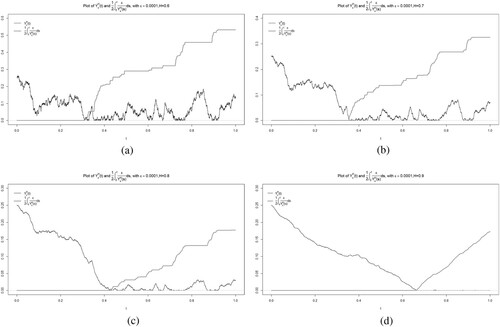
Theorem 3.1 states that the grey line approximates the reflection function of the RFOU process and it can be clearly seen that the plot is well agreed with the theory: the integral
shows notable growth only when the corresponding path of
is very close to zero.
Figure illustrates the uniform convergence of paths of to the path of RFOU process as
. On the picture, H = 0.6,
, b = 1,
and the path of the FROU process
was simulated using the Euler-type method:
Figure 2. Comparison of the with
,
,
,
(lines with colors ranging from light grey to dark grey) and the RFOU process (bold black line). Note that the purple path (
) is not visible on the plot since it almost completely coincides with the bold black trajectory of the RFOU process.
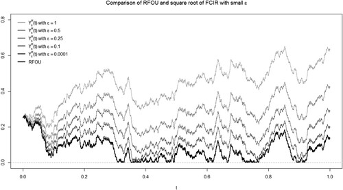
When , the path of
is so close to the corresponding path of the ROU process (bold black) that they are not distinguishable on the plot.
Acknowledgments
The present research is carried out within the frame and support of the ToppForsk project nr. 274410 of the Research Council of Norway with title STORM: Stochastics for Time-Space Risk Models. The first author is supported by the National Research Fund of Ukraine under grant 2020.02/0026.
Disclosure statement
No potential conflict of interest was reported by the author(s).
Additional information
Funding
References
- O.O. Aalen and H.K. Gjessing, Survival models based on the Ornstein-Uhlenbeck process, Lifetime Data Anal. 10 (2004), pp. 407–423.
- C.A. Ball and A. Roma, Stochastic volatility option pricing, J. Financ. Quantitative Anal. 29 (1994), pp. 589–607.
- L. Bo, D. Tang, Y. Wang and X. Yang, On the conditional default probability in a regulated market: a structural approach, Quantitative Financ. 11 (2011), pp. 1695–1702.
- L. Bo, Y. Wang and X. Yang, Some integral functionals of reflected SDEs and their applications in finance, Quantitative Financ. 11 (2011), pp. 343–348.
- J.C. Cox, J.E. Ingersoll and S.A. Ross, A re-examination of traditional hypotheses about the term structure of interest rates, The J. Financ. 36 (1981), pp. 769–799.
- J.C. Cox, J.E. Ingersoll and S.A. Ross, An intertemporal general equilibrium model of asset prices, Econometrica: J. Econ. Soc. 53 (1985), pp. 363.
- J.C. Cox, J.E. Ingersoll and S.A. Ross, A theory of the term structure of interest rates, Econometrica: J. Econom. Soc. 53 (1985), pp. 385.
- G. Di Nunno, Y. Mishura and A. Yurchenko-Tytarenko, Sandwiched SDEs with unbounded drift driven by Holder noises, preprint (2020), Available at ArXiv 2012.11465.
- V. Giorno, A.G. Nobile and R. di Cesare, On the reflected Ornstein-Uhlenbeck process with catastrophes, Appl. Math. Comput. 218 (2012), pp. 11570–11582.
- V. Giorno, A.G. Nobile and L.M. Ricciardi, On some diffusion approximations to queueing systems, Adv. Appl. Probab. 18 (1986), pp. 991–1014.
- R.S. Goldstein and W.P. Keirstead, On the term structure of interest rates in the presence of reflecting and absorbing boundaries, preprint (1997). doi:10.2139/ssrn.19840.
- S.L. Heston, A closed-form solution for options with stochastic volatility with applications to bond and currency options, Rev. Financ. Stud. 6 (1993), pp. 327–343.
- J. Hong, C. Huang, M. Kamrani and X. Wang, Optimal strong convergence rate of a backward Euler type scheme for the Cox-Ingersoll-Ross model driven by fractional Brownian motion, Stoch. Process. Appl. 130 (2020), pp. 2675–2692.
- N. Ikeda and S. Watanabe, A comparison theorem for solutions of stochastic differential equations and its applications, Osaka J. Math. 14 (1977), pp. 619–633.
- N. Ikeda and S. Watanabe, Stochastic Differential Equations and Diffusion Processes, Elsevier, 1981.
- I. Karatzas and S.E. Shreve, Brownian Motion and Stochastic Calculus, Springer, New York, 1998.
- P.R. Krugman, Target zones and exchange rate dynamics, The Quarterly J. Econ. 106 (1991), pp. 669–682.
- K. Kubilius, Estimation of the Hurst index of the solutions of fractional SDE with locally Lipschitz drift, Lithuanian Association of Nonlinear Analysts (LANA). Nonlinear Analysis. Modelling and Control 25 (2020), pp. 1059–1078.
- C. Lee and J. Song, On drift parameter estimation for reflected fractional Ornstein-Uhlenbeck processes, Stoch. An Int. J. Probab. Stoch. Process. 88 (2016), pp. 751–778.
- V. Linetsky, On the transition densities for reflected diffusions, Adv. Appl. Probab. 37 (2005), pp. 435–460.
- Y. Maghsoodi, Solution of the extended CIR term structure and bond option valuation, Math. Financ. An Int. J. Math., Stat. Financial Econom. 6 (1996), pp. 89–109.
- A. Melnikov, Y. Mishura and G. Shevchenko, Stochastic viability and comparison theorems for mixed stochastic differential equations, Methodol. Comput. Appl. Probab. 17 (2015), pp. 169–188.
- Y. Mishura and A. Yurchenko-Tytarenko, Fractional Cox-Ingersoll-Ross process with non-zero “mean”, Modern Stoch.: Theor. Appl. 5 (2018), pp. 99–111.
- V.I. Piterbarg, Twenty Lectures About Gaussian Processes, Atlantic Financial Press, 2015.
- L.M. Ricciardi, Stochastic population theory: Diffusion processes, Mathematical Ecology, Springer, Berlin Heidelberg, (1986), pp. 191–238.
- L.C.G. Rogers and D. Williams, Diffusions, Markov Processes and Martingales, Cambridge University Press, 2000.
- R. Schöbel and J. Zhu, Stochastic volatility with an Ornstein-Uhlenbeck process: an extension, Rev. Financ. 3 (1999), pp. 23–46.
- T. Shiga and S. Watanabe, Bessel diffusions as a one-parameter family of diffusion processes, Zeitschrift fur Wahrscheinlichkeitstheorie und Verwandte Gebiete 27 (1973), pp. 37–46.
- A.V. Skorokhod, Stochastic equations for diffusion processes in a bounded region, Theor. Probab. Appl. 6 (1961), pp. 264–274.
- A.R. Ward and P.W. Glynn, A diffusion approximation for a Markovian queue with reneging, Queueing Syst. 43 (2003), pp. 103–128.
- A.R. Ward and P.W. Glynn, Properties of the reflected Ornstein-Uhlenbeck process, Queueing Syst.44 (2003), pp. 109–123.
- A.R. Ward and P.W. Glynn, A diffusion approximation for a GI/GI/1 queue with balking or reneging, Queueing Syst. 50 (2005), pp. 371–400.
- X. Yang, X. Li, G. Ren, Y. Wang and L. Bo, Modeling the exchange rates in a target zone by reflected Ornstein-Uhlenbeck process, SSRN Electron. J. (2012), 10.2139/ssrn.2107686.
- D. Ylvisaker, A note on the absence of tangencies in Gaussian sample paths, Ann. Math. Stat. 39 (1968), pp. 261–262.
- M. Zähle, Integration with respect to fractal functions and stochastic calculus. I, Probability Theory and Related Fields 111 (1998), pp. 333–374.
- S.Q. Zhang and C. YuanStochastic differential equations driven by fractional Brownian motion with locally Lipschitz drift and their implicit Euler approximation, Proceedings of the Royal Society of Edinburgh: Section A Mathematics, (2020), pp. 1–27.
- J. Zhu, Applications of Fourier Transform to Smile Modeling, Springer, Berlin Heidelberg, 2010.