Unsteady RANS and IDDES studies on a telescopic crescent-shaped wingsail

ABSTRACT

Over the years, several research projects have evaluated different concepts for wind-assisted propulsion, generally concluding that it can lead to significant fuel savings. The time-averaged propulsive performance of a single rigid wingsail has been analysed in previous studies. However, the unsteady characteristics of the external loads which may induce structural vibration are also important to be considered. In this study, full-scale simulations, with both unsteady RANS and IDDES methods, are performed to analyze the flow field. The paper's analysis includes flow separation and vortex shedding, the development and dissipation of wake vortices, and the lift reduction due to tip vortices. It also studies the telescopic function of the wingsail by analyzing sails with different heights and wind conditions. The paper concludes that the unsteady RANS and IDDES simulations make similar predictions for time-averaged loads but disagree on the unsteady characteristics. The IDDES simulations indicate more complex vortex-shedding phenomena.

KEYWORDS:

• Flow separation
• IDDES
• unsteady RANS
• wake analysis
• wind-assisted ship propulsion

1. Introduction

Transportation accounts for a large proportion of greenhouse gas emissions. According to the data of 2017, transportation shared $24\text{\%}$ of the EU greenhouse gas emission (Eurostat 2019). On the basis of the statistical data in 2014, approximately $90\text{\%}$ of world trade volume is transported by shipping fleets (International Chamber of 2014). The International Maritime Organisation (IMO) has agreed on a target to reduce greenhouse gas emissions from shipping by $50\text{\%}$, relative to 2018 levels, by 2050 (IMO 2018). The use of wind-assisted ship propulsion is regarded as a promising means to help achieve this goal. Over the years, several projects have been carried out to develop and evaluate different concepts for wind-assisted propulsion systems using rigid wingsails and have found that they can reduce fuel consumption by over $30\text{\%}$ (Hamada 1985). Unlike kite sails, rigid wingsails can not only propel ships by the drag force but also the lift force, enabling ships to navigate against the wind (Kimball 2009). An ongoing project, Oceanbird (Workinn 2021), even aims to achieve a $90\text{\%}$ fuel reduction, which is much higher than the typical savings from Flettner rotors, which are $8\text{\%}$ on average (International Transport 2020), $30\text{\%}$ for tankers (Tillig and Ringsberg 2020), and around $50\text{\%}$ at maximum (Traut et al. 2014). Due to the bluff body, Flettner rotors suffer from high drag, resulting in extra resistance when the rotors are not operating (Khan et al. 2021). In addition, rigid wingsails show better propulsive performance than Flettner rotors under downwind conditions, in which the drag force contributes to the propulsion (Lu and Ringsberg 2020). Compared with traditional soft sails, the main advantages of rigid wingsails are that they maintain their shape in light winds and are more robust to control since there is no rope that could become entangled (Sauzé and Neal 2008). They also have simpler structures and are easier to design and manufacture (Silva et al. 2019).

The key characteristic of a propulsion system is its propulsive performance. In addition to empirical studies or experimental tests, such as wind tunnel tests, numerical simulations are seen as an efficient way to predict propulsive performance. In recent years, several researchers have developed numerical methods to study rigid wingsails based on airfoil profiles. Lee et al. (2016) studied a series of rigid wingsails based on the NACA 0012 profile, carried out numerical aerodynamic analysis using a viscous Navier–Stokes flow solver, and established a design optimisation framework to maximise the thrust coefficient, $C_T$. Ma et al. (2018) studied three typical airfoil-based sails by computational fluid dynamics (CFD) simulations, using the $k-\omega$ shear stress transport (SST) turbulence model. Blount and Portell (2021) studied a concept based on the NACA 0015 profile using the improved delayed detached eddy simulation (IDDES) method and discussed the vortex shedding under downwind conditions. These conventional sectional profiles provide effective propulsion, but an even higher $C_T$ needs to be obtained to achieve the IMO target. It has been found that aerodynamically asymmetric profiles, such as segment-shaped (Atkinson 2019) or crescent-shaped (Nikmanesh 2021) profiles, show better propulsive performance than conventional designs.

However, as predicted by unsteady Reynolds-averaged Navier–Stokes equations (uRANS) CFD simulations (Zhu et al. 2022), the notable camber of these profiles leads to significant flow separation and an unsteady flow field, which is challenging to capture using numerical models. Moreover, when considering the structural response, it is important to consider not only the time-averaged loading conditions but also oscillations in the loads, which can induce a global flutter or local vibrations. To analyze vortex-induced vibrations (VIV), it is necessary to accurately predict the frequency of the oscillations in the external loads. In addition, there is usually more than one sail installed on a ship, and the wake flow of the upstream sail will likely have an influence on the downstream sails. Therefore, an improved CFD model needs to be established to understand the unsteady properties and the wake flow.

The current study, which is a continuation of previous work (Zhu et al. 2022), investigates a concept design of a telescopic rigid wingsail with a crescent-shaped profile using CFD. The main objective is to study the unsteady characteristics of the wind loads on the wingsail and the induced flow field. Numerical simulations based on the IDDES method with uRANS simulations are performed and compared to provide an accurate numerical model for predicting unsteady characteristics of the wind loads. It was found that by applying the IDDES method, more detailed information about the flow field can be obtained, especially the flow separation and the vortex shedding. In addition, the telescopic function of the wingsail and possible optimisation of the tip geometry are also presented.

2. Methodology

2.1. Concept design

2.1.1. Crescent-shaped section

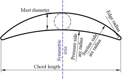
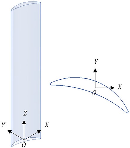
In this study, the horizontal section profile of the wingsail, illustrated in Figure 1, is a simple crescent shape, made up of arcs and circles. There are four main design parameters: the chord length, the edge radius, the suction-side arc radius, and the mast diameter. The shape of the profile, including the pressure-side arc radius, is determined by these four parameters. The arcs of the pressure side and suction side are symmetric about the symmetric axis (the dashed blue line in Figure 1). The radius of the edges is chosen to make the profile structurally sound.

Figure 1. Design parameters of the crescent-shaped profile. This figure is available in colour online.

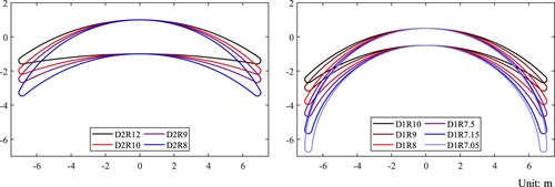
A parametric sensitivity analysis is carried out. The mast diameter and the suction-side arc radius are adjusted. The chord length is always set at $14\mathrm{m}$, and the edge radius is always $0.2\mathrm{m}$. A series of profiles (shown in Figure 2) are generated by varying the remaining two parameters and are labeled in the form ‘DxRy', where ‘x' represents the mast diameter and ‘y' represents the suction-side arc radius. For example, for the profile named ‘D2R8', the mast diameter is $2\mathrm{m}$ and the suction-side arc radius is $8\mathrm{m}$, which results in an arc radius of $10.67\mathrm{m}$ on the pressure side.

Figure 2. Crescent-shaped profiles based on different design parameters. This figure is available in colour online.

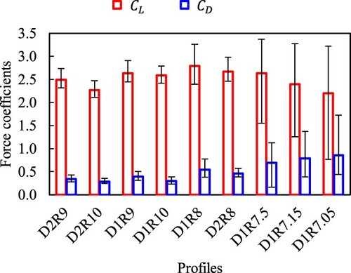
Figure 3 shows the results of two-dimensional unsteady RANS simulations for several different profiles. The numerical and physical setups of the two-dimensional simulations follow a previous study by the authors (Zhu et al. 2022). The error bars in Figure 3 represent the oscillation amplitudes. Clearly, as the camber increases, the drag coefficient $C_D$ increases while the lift coefficient $C_L$ initially increases and then decreases. For profiles with extreme camber, such as D1R7.5, the oscillation of the force coefficients becomes very strong. The profiles D2R8 and D1R8 show the highest time-averaged lift force coefficient but the loads on D1R8 show much larger oscillations. By considering the structural arrangements, a mast with a larger diameter is expected to provide better strength, so the D2R8 profile is selected for this study.

Figure 3. Force coefficients of different profiles. This figure is available in colour online.

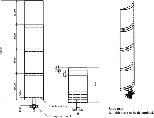
2.2. Telescopic function

The rig is designed to have a telescopic function to enable reefing of the wingsails depending on the wind conditions, as shown in Figure 4. The wingsail is divided into four sections, which can be retracted or expanded. For example, at low wind speeds, such as $8\mathrm{m}/\mathrm{s}$, the wingsail would be expanded to generate maximum propulsion, while for conditions with higher wind speeds, such as $32\mathrm{m}/\mathrm{s}$, it would be retracted to prevent structural failures. The fully expanded height of the wingsail is $74\mathrm{m}$, while the fully retracted height is $26\mathrm{m}$. The wingsail is supported by a mast that is fixed to the deck. In the preliminary design, the total height of the mast is $6\mathrm{m}$, with $2\mathrm{m}$ inside the sail.

Figure 4. Concept design of the telescopic rigid wingsail. This figure is available in colour online.

2.3. Physical conditions

In the CFD simulations, the wingsail is modelled as a uniformly extruded rigid body. As mentioned in Section 2.2, the height of the wingsail can be adjusted according to the apparent wind speed. Two conditions are simulated, the fully expanded condition and the fully retracted condition, with the parameters listed in Table 1.

Table 1. Height and apparent wind speed of the two simulated conditions.

Condition	$V_{AW}$	$H$
Fully expanded	$8\mathrm{m}/\mathrm{s}$	$74\mathrm{m}$
Fully retracted	$32\mathrm{m}/\mathrm{s}$	$32\mathrm{m}$

Table 2 shows the properties of the fluid (air at ${25}^{\circ }\mathrm{C}$ (Hilsenrath 1955)). Since the chord length of the section is $14\mathrm{m}$, $Re$ is $6.78\times {10}^6$ for the fully expanded condition and $2.71\times {10}^7$ for the fully retracted condition.

Table 2. Properties of the fluid (air at ${25}^{\circ }\mathrm{C}$ (Hilsenrath 1955)).

Property	Value	Unit
$\mu$	$1.85508\times {10}^{-5}$	$\mathrm{P}\mathrm{a}\cdot \mathrm{s}$
$\rho$	$1.18415$	$\mathrm{k}\mathrm{g}/{\mathrm{m}}^3$

The global coordinate system, as shown in Figure 5, is defined such that the origin is located at the bottom surface at the centre of the mean camber line, i.e. the half-thickness point at the mid-chord. The $X$-axis is parallel to the streamwise direction and has the same direction as the inlet flow. The $Y$-axis represents the crossflow direction, pointing from the pressure side to the suction side. The $Z$-axis points vertically from the bottom to the top, representing the spanwise direction.

Figure 5. Coordinate system. This figure is available in colour online.

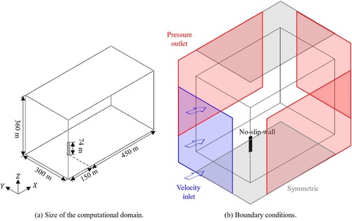
The calculation domains for the two conditions have the same size, as shown in Figure 6. The top and bottom of the domain have symmetric boundary conditions. The upstream panel is treated as a velocity inlet with uniformly distributed inlet flow, representing the apparent wind. The direction of the inlet flow can also be seen in Figure 6. The downstream panel and the crossflow sides are treated as pressure outlets. To avoid the influence of the reversed flow at pressure outlet boundaries, the direction of the backflow is set to be extrapolated. The pressure loss at the pressure outlets is assumed to be $0$, and the pressure jump under-relaxation factor is set as $0.5$.

Figure 6. Computational domain and boundary conditions, fully expanded condition. This figure is available in colour online.

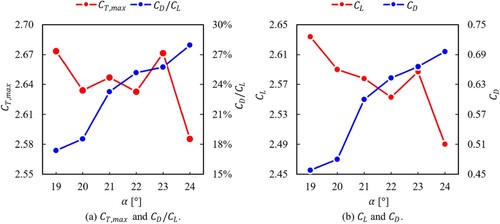
Unlike conventional airfoils, flow separation phenomena can be found even when the angle of attack $\alpha =0^{\circ }$, so there is no specific stall angle. Instead, the $C_L$ is damped across a range of $\alpha$ values. Initial two-dimensional CFD simulations are performed to find the critical angle of attack ${\alpha }_c$ (results shown in Figure 7), based on which three-dimensional CFD simulations are performed. In the two-dimensional CFD simulations, the maximum $C_L$ is obtained when $\alpha ={19}^{\circ }$. There is also a lower peak in $C_L$ when $\alpha ={23}^{\circ }$. Within the range studied, $C_D$ shows a positive correlation with $\alpha$. If only the lift force is considered, ${19}^{\circ }$ should be the optimum angle of attack. However, for this sectional profile, the contribution of the drag force to the thrust cannot be ignored since the ratio between drag and lift is around $17-29\text{\%}$. By considering the maximum $C_T$ value $C_{T,max}=\sqrt{C_L^2+C_D^2}$, two peaks are found at $\alpha ={19}^{\circ }$ and $\alpha ={23}^{\circ }$. Therefore, in this study, three-dimensional CFD simulations are performed based on three values of $\alpha$, namely, ${19}^{\circ }$, ${21}^{\circ }$, and ${23}^{\circ }$.

Figure 7. Time-averaged force coefficients vs. $\alpha$, based on two-dimensional CFD simulations. This figure is available in colour online.

2.4. Mesh

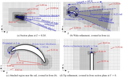
An unstructured mesh with a trimmed cell topology (Siemens PLM Software 2021) is applied for the uRANS and IDDES numerical simulations. Prism layers are generated near the walls to resolve the flow in the boundary layers. Figure 8 shows the trimmed mesh in the sectional planes of $Z=0.5H$ and $Y=0$ (the half chord). The mesh is refined with eight levels in addition to the prism layers. According to previous studies (Zhu et al. 2022), the flow field around the crescent-shaped foil displays significant flow separation phenomena. Flow separation is induced by both the trailing edge and the leading edge. Therefore, local refinement is applied to the wake region, the region close to the tip, and the region around the foil, especially in areas close to the two edges. The angle between the direction of the wake refinement and the streamwise direction is $0.5\alpha$ (see Figure 8(a)). The length of the wake refinement is $60\mathrm{m}$, and the separating angle is $0.25\mathrm{r}\mathrm{a}\mathrm{d}$, as shown in Figure 7(b). For the cells in the wake region, the size is around $0.32\mathrm{m}$. As shown in Figure 8(c), the size of cells is $0.08\mathrm{m}$ for those close to the edges, and the thickness of the prism layer is $0.5\mathrm{m}$ with 65 layers inside. To study the characteristics of the tip vortices, the mesh around the free-stream tip is also refined, as shown in Figure 8(d).

Figure 8. Numerical mesh with typical cell sizes. Fully expanded condition with $\alpha ={19}^{\circ }$. This figure is available in colour online.

The global mesh topology and refinement strategy was based on a mesh independence study presented in (Zhu et al. 2022). For the IDDES simulations, the mesh independence studies were conducted based on the fully expanded condition. Three sets of meshes with different refinement levels were studied. It was found that the difference in time-averaged $C_L$ between the finest mesh (42 million cells) and the medium mesh (23 million cells) is $0.23\text{\%}$, the difference between the finest mesh and the coarsest mesh (14 million cells) is $2.06\text{\%}$. Thus, the medium mesh was used for further studies. The total number of cells for the fully expanded condition is about 23 million, while for the fully retracted condition, it is around 8 million.

2.5. Numerical model

2.5.1. Viscous regimes

To solve this high-$Re$ problem, turbulence models need to be incorporated. In the previous study (Zhu et al. 2022), a CFD model based on the uRANS method was developed, and the time-averaged loading conditions were well solved since the boundary-layer flow was resolved with a finely layered mesh. However, significant flow separation was found, which leads to significant unsteady characteristics of the flow field. When studying the propulsive performance of a single sail, it is enough to only consider the time-averaged loads. However, the unsteady characteristics should be considered when analyzing the structural response. For example, a low-frequency oscillation of the external loads may cause vortex-induced vibration of the whole sail, while a high-frequency oscillation may cause local vibrations on the shell panels, resulting in buckling. To simulate the separating flow more accurately, the large eddy simulation (LES) method (Smagorinsky 1963) needs to be introduced, since all turbulent scales are modelled in uRANS, while only small, isotropic turbulent scales are modelled in LES (Davidson 2019). By applying the LES method, both the time-averaged properties and the unsteady characteristics can be determined. On the other hand, the LES method imposes costly near-wall meshing requirements. To avoid that and keep the boundary-layer flow well-resolved, the detached eddy simulation (DES) method, which combines uRANS and LES, is selected in this study.

The $k-\omega$ SST model (Menter 1993) is applied for both the uRANS and IDDES (Shur et al. 2008) simulations. The turbulence eddy viscosity is computed based on the turbulence kinetic energy and the specific turbulence dissipation rate. The convection term of the model is discretized with a second-order upwind scheme. The $k-\omega$ SST model interprets the standard $k-\omega$ model within the inner layer of the boundary condition. When reaching the free shear layers, it switches to the $k-ϵ$ model to reduce the sensitivity for the inlet free-stream properties.

With the goal of precisely predicting the flow separation, the IDDES method relating to a hybrid RANS–LES approach, is also used in the simulation compared with uRANS results. With the aim to alleviate the costly near-wall meshing requirements imposed by LES, the boundary-layer flow is treated with RANS and the outer detached eddies are captured by LES.

To clarify the importance of introducing DES-type methods, a pair of fluid–structure interaction (FSI) simulations are performed using uRANS and IDDES, assuming that the sail is a solid aluminum body fixed at its bottom, i.e. a cantilever boundary condition. The properties of the material are listed in Table 3. Since the stress is relatively low, compared with the yield stress, only elastic deformation is considered in these cases. Finite element method (FEM) is used for calculating the structural response of the solid body. The commercial software ABAQUS (Dassault 2020) is used to perform the FEM simulations, and the analysis product is ABAQUS/Standard. A set of quad-dominated mesh is applied to the FEM model. In these cases, $\alpha$ is set as ${23}^{\circ }$. The FSI simulation uses a two-way coupling approach, meaning that at every time step, the wall pressure and shear stress is transferred from CFD model to FEM model, and the deformation displacement is transferred from FEM model to CFD model.

Table 3. Material properties.

Material	$\rho$	$E$	$\upsilon$	${\sigma }_{yield}$
	[$\mathrm{k}\mathrm{g}/{\mathrm{m}}^3$]	[$\mathrm{G}\mathrm{P}\mathrm{a}$]	[-]	[$\mathrm{M}\mathrm{p}\mathrm{a}$]
Al (6061-T4) (ASTM 2004)	$2700$	$69$	$0.33$	$210$

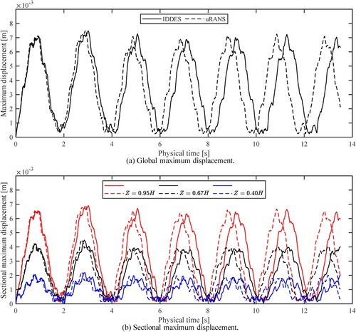
Figure 9(a) presents the global maximum displacement of the structure deformation ($w$), where $w$ is the magnitude of the displacement, i.e. $w=\sqrt{w_X^2+w_Y^2}$. The maximum global displacement always happens at the tip of the wingsail. Figure 9(b) presents the maximum displacement of horizontal sections at different spanwise positions. At the very beginning, since very few cells are calculated by LES, the two methods show very similar results. As physical time goes on, more discretized cells are assigned in the LES region and the differences between the two methods become significant. The uRANS results show a larger damping amplitude: there is a difference in the peak value of around $15\text{\%}$ between the two methods. The IDDES results show more high-frequency damping, especially at the lower part of the sail (see the black and blue lines in Figure 9(b)). Shell structures, such as the concept design in Figure 4, are expected to be more sensitive to high-frequency oscillations, so LES or DES-type simulations are necessary.

Figure 9. Deformation displacement ($w$) from FSI results. $w$ is the magnitude of displacement, i.e. $w=\sqrt{w_X^2+w_Y^2}$. This figure is available in colour online.

Take the fully expanded condition with $\alpha ={23}^{\circ }$ as an example. Figure 10 shows the distribution of regions calculated by uRANS and LES. Most areas, especially the boundary flow regions, are calculated by uRANS. The LES regions are mainly distributed in the downstream field. Due to the impact of the tip vortices, fewer areas are calculated by LES when approaching the tip (see Figure 10(a)). This explains why the lower part of the sail shows a more high-frequency structural response in Figure 9.

Figure 10. Distribution of DES upwind blending factor at different spanwise positions, fully expanded condition, $\alpha ={23}^{\circ }$. Blue marks out the regions calculated with LES, while the rest of the computation domain is calculated with uRANS. This figure is available in colour online.

The approach of blended wall treatment, which is useful in treating complex geometries with local flow characteristics, is applied to the RANS equations. The traditional low-$Re$ approach is applied, in which the boundary layer is resolved with a finely layered mesh. In the simulations, the order of magnitude of $y^{+}$ on most areas of the wall is around ${10}^{-1}$, with the purpose of having a more detailed and accurate representation of the boundary-layer flow.

2.5.2. Solvers and discretization schemes

A finite volume method (FVM) is used to discretize the governing equations by employing a segregated flow solver. The numerical solver uses the Semi-Implicit Method for Pressure-Linked Equations (SIMPLE) algorithm (Patankar 1981). In STAR-CCM+, this is called the ‘implicit unsteady solver'. The freestream Mach number is less than $0.1$, so the flow is regarded as incompressible flow with constant density. A second-order implicit method is used to discretize the time derivative. The scale of the time step is $2\times {10}^{-4}\mathrm{s}$ to keep the Courant number under $10$, since an implicit solver is applied. A hybrid second-order upwind scheme and the bounded-central scheme are used to discretize the convection fluxes. The diffusion fluxes are discretized with a second-order scheme. The gradient computation uses the second-order hybrid Gauss-LSQ method.

3. Results and discussion

3.1. Propulsive performance

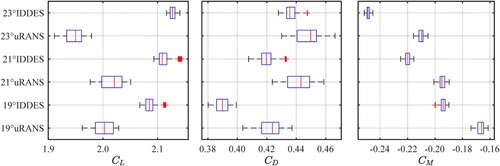
The force coefficients, representing the external loads on the sail, are analysed to study the propulsive performance of the rigid wingsail. As can be seen in Figure 11, which presents the boxplots of the force coefficients under the fully expanded condition, the uRANS and IDDES methods provide similar results for the time-averaged force coefficients. The difference between these two methods is usually less than $10\text{\%}$ for $C_L$ (Figure 11(a)) and $C_D$ (Figure 11(b)), and $15\text{\%}$ for $C_M$ (Figure 11(c)). On the other hand, as mentioned in Section 2.5.1, it is believed that IDDES simulations predict the unsteady characteristics, especially high-frequency properties of the external loads, more accurately due to the strong flow separation phenomena. Based on the IDDES results, it can be concluded that in the studied range of $\alpha$, the highest $C_L$ is around $2.102$ at $\alpha ={23}^{\circ }$. Simulations of the fully retracted condition suggest the same optimal $\alpha$. The value of $C_D$, which also contributes to the thrust at board reach, is also higher when $\alpha ={23}^{\circ }$. However, the force coefficients from the uRANS simulations show significantly larger oscillation amplitudes, especially for $C_L$. The reason for this is explained in Section 3.2.

Figure 11. Boxplots of time-averaged force coefficients, fully expanded condition. This figure is available in colour online.

Table 4 presents the time-averaged value of the force coefficients based on the IDDES simulations. $C_L$ is around $10\text{\%}$ higher under the fully expanded condition, while the $C_D$ values are approximately $17-27\text{\%}$ lower. The reason is that when the rigid wingsail is fully retracted, the impact from the tip vortices is much stronger, leading to reduced lift. Section 3.4 discusses the characteristics of the tip vortices and presents some solutions to reduce the negative impacts.

Table 4. Time-averaged force coefficients based on IDDES simulations.

Condition	$\alpha$ [${}^{\circ }$]	$C_L$	$C_D$	$C_M$
Fully expanded condition	19	2.085	0.390	−0.194
	21	2.111	0.420	−0.220
	23	2.128	0.437	−0.247
Fully retracted condition	19	1.889	0.488	−0.106
	21	1.879	0.510	−0.131
	23	1.914	0.534	−0.161

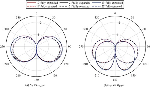
Based on the time-averaged values of force coefficients from the IDDES simulations, the propulsive performance can be predicted. A single rigid wingsail can provide up to $86\mathrm{k}\mathrm{N}$ of thrust force under the fully expanded condition, and $444\mathrm{k}\mathrm{N}$ under the fully retracted condition. Figure 12 presents $C_T$ at different apparent wind and true wind directions. The value of $V_S$ is $12\mathrm{k}\mathrm{n}$ (around $6.2\mathrm{m}/\mathrm{s}$). $V_{TW}$ is fixed separately at $8\mathrm{m}/\mathrm{s}$ and $32\mathrm{m}/\mathrm{s}$ for the fully expanded condition and fully retracted conditions, respectively. Although $Re$ varies with the true wind direction, the force coefficients are assumed to remain the same since they are not sensitive to $Re$. The trend of $C_T$ with different apparent wind directions is similar between the fully expanded condition and the fully retracted condition, as Figure 12(a) shows. It can be seen that the wingsail does not work when ${\theta }_{AW}<{30}^{\circ }$, which is the luffing point of sail (Rousmaniere 1999). As shown in Figure 12(b), for the fully retracted condition, the rigid wingsail attains its best propulsive performance when ${\theta }_{TW}$ is $90-{120}^{\circ }$, that is, when the point of sail is a beam reach. However, for the fully expanded condition, the maximum $C_T$ is obtained when ${\theta }_{TW}$ is around ${160}^{\circ }$, which is close to the downwind condition.

Figure 12. Polar diagram of $C_T$ vs. wind directions. This figure is available in colour online.

3.2. Flow separation

The flow field induced by the crescent-shaped profile has a remarkable flow separation phenomenon at the suction side close to the trailing edge, which is the reason for the unsteady characteristics. To reduce the influence of the tip vortices (discussed in Section 3.4), the analysis of the flow separation and vortex shedding is based on the fully expanded condition. For clearer presenting and discussing the flow separation phenomenon, the simulation case with the largest $\alpha$, i.e. $\alpha ={23}^{\circ }$, is taken as the example.

Figure 13, which presents the streamwise velocity distribution and the streamline at the sectional plane with different spanwise positions, shows that the results from uRANS and IDDES share some similarities. For upstream areas of the half chord, that is, on the left of the half chord in the subfigures of Figure 13, the flow is resolved by applying the $k-\omega$ SST turbulence model when using both the uRANS and IDDES methods. Therefore, the characteristics of the flow field predicted by the two methods are almost the same. There is a high-velocity region where the streamwise velocity is approximately twice the inlet flow velocity, on the suction side upward of the half chord, which causes a reduction of pressure and finally leads to the lift force. There is a pronounced low-velocity region on the suction side of the profile, extending to the downstream areas. The observed phenomena support the hypothesis that the IDDES method provides more detailed information on the separating flow since the large eddies are directly resolved instead of being modelled.

Figure 13. $V_X$ distribution and streamlines at different spanwise sections, fully expanded condition, $V_{AW}=8\mathrm{m}/\mathrm{s}$, $\alpha ={23}^{\circ }$. This figure is available in colour online.

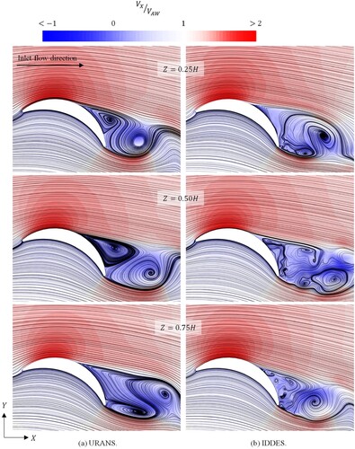
As shown in Figure 10, the low-velocity region is mainly calculated by LES when applying the IDDES method. Therefore, the flow field in this area shows some differences between the two methods. The results based on the uRANS method show two main vortices (see Figure 13(a)). At the lower part of the sail, for instance $Z=0.25H$, the IDDES results also show the main vortices, because the bottom panel with the symmetric boundary condition constrains vortex development in the spanwise direction. However, at the higher part of the sail, such as $Z=0.50H$ and $Z=0.75H$, the flow shows more complex characteristics in the IDDES results (see Figure 13(b)).

The pressure distributions on the surface of the rigid wingsail are shown in Figure 14 alongside the flow separation/attachment lines. There are multiple flow separation points on the suction side close to the trailing edge. For the IDDES results, the distribution of the flow separation lines shows random properties in the spanwise direction, which further explain the complex separating flow in Figure 13(b). The flow separation areas narrow in the crossflow direction when the position is near the tip because of the phenomenon of tip vortices. There are also some flow separation/attachment lines on the pressure side near the edges.

Figure 14. $C_p$ distributions and the flow separation/attachment lines, $\alpha ={23}^{\circ }$. For the fully expanded condition, $V_{AW}=8\mathrm{m}/\mathrm{s}$, while for the fully retracted condition, $V_{AW}=32\mathrm{m}/\mathrm{s}$. This figure is available in colour online.

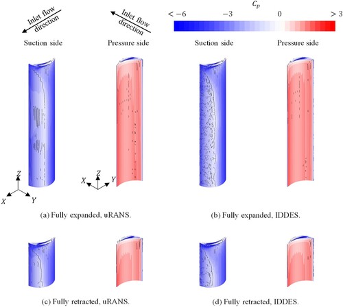
Although the flow separation lines are not uniformly developed, the pressure coefficient is evenly distributed along the spanwise direction, except in the region near the tip. The low-pressure areas located at the suction side approaching the leading edge coincide with the high-velocity areas in Figure 13, which mainly contribute to the lift force. It can be inferred that the loads on the surface of the rigid wingsail will make the structure suffer from deformation, especially bending. Meanwhile, the multiple flow separation points cause oscillations of the external loads, which may lead to vortex-induced vibrations.

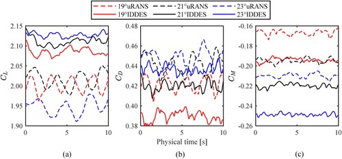
Periodic oscillations are evident from the time history of the $C_L$ values in the uRANS simulations, presented in Figure 15(a). In contrast, the oscillations are quite random, without a clear period, in the IDDES simulations. Referring to the FSI simulations in Section 2.5.1, these irregular oscillations explain the high-frequency damping found in the IDDES results.

Figure 15. Simulation time history of the force coefficients, fully expanded condition. This figure is available in colour online.

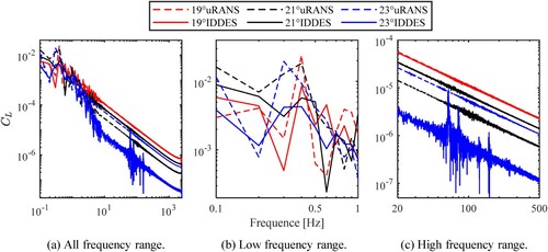
Therefore, to study the unsteady properties of the force coefficients, FFT analysis is conducted. Figure 16 presents the FFT analysis results for $C_L$ under the fully expanded condition. The length of physical time of the selected data is $10\mathrm{s}$, so the first peak with the frequency of $0.1\mathrm{H}\mathrm{z}$ is spurious and can be ignored. When looking at the dashed lines, a second set of peaks is evident with frequencies around $0.4\mathrm{H}\mathrm{z}$, so the uRANS simulations indicate that $C_L$ has a clear oscillating period of $2.5\mathrm{s}$ and an amplitude of approximately $0.02$. The $C_L$ values predicted by the IDDES simulations do not show periodic oscillations. In Figure 16(b), in which the FFT plot is zoomed in at the low-frequency region, the second set of peaks is unclear for the solid lines. Some small oscillations can also be found on the solid lines in the high-frequency region of the FFT results, shown in Figure 16(c). The time history and FFT results of $C_D$ and $C_M$, as well as those under the fully retracted condition, show similar characteristics.

Figure 16. FFT results of $C_L$, fully expanded condition. This figure is available in colour online.

3.3. Wake flow

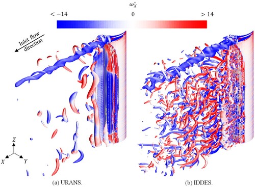
Normally, more than one wingsail is installed and operated on a ship. The analysis of the wake flow is expected to provide some guidance in future studies on ships with multiple sails. The wake flow resolved by the two methods shows many differences. In this Section, results under fully expanded condition are selected as samples. The IDDES simulations predict a flow field with much more complex vortex structures, as shown in Figure 17, which shows the distribution of ${\omega }_X^{\ast }$ on the iso-surfaces of $Q=5{\mathrm{s}}^{-2}$. From the uRANS simulations, as Figure 17(a) shows, the spanwise vortex tubes can be easily observed, which means that the vortex shedding phenomena do not show significant spanwise characteristics, except for the tip vortices. However, the vortices have numerous streamwise and crossflow structures when applying the IDDES method, as shown in Figure 17(b). These complex vortex structures lead to the unclear oscillating period described in Section 3.2.

Figure 17. Non-dimensional ${\omega }_X$ distribution on iso-surfaces of the Q-criterion $Q=5{\mathrm{s}}^{-2}$, fully expanded condition, $V_{AW}=8\mathrm{m}/\mathrm{s}$, $\alpha ={23}^{\circ }$. This figure is available in colour online.

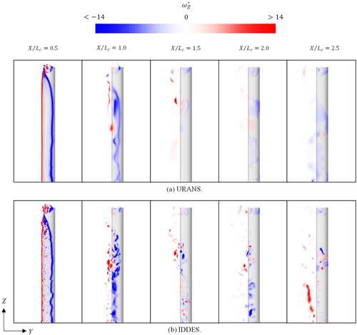
When looking at the ${\omega }_Z$ distribution at section planes with different streamwise positions, shown in Figure 18, the differences between the results simulated by the two methods are more readily apparent. The uRANS results show some vertical vortex tubes: for example, in Figure 18(a), when $X/L_C=0.5$, that is, just behind the trailing edge, a strong vortex tube can be found. However, when using the IDDES method (see Figure 18(b)), there are small vortices on the decimeter scale at the section plane of $X/L_C=0.5$. When looking at the position $X/L_C=1.0$, the distribution of ${\omega }_Z$ is preserved in Figure 18(a), while for the IDDES results, it can only be found in the lower part close to the bottom panel. Moreover, the vortices dissipate quickly in the wake region when applying the uRANS method, which indicates that there is more energy loss. The turbulent kinematic energy in the wake region is much lower when applying the IDDES method. When looking at the streamwise position of $X/L_C=2.0$, the vortices predicted by the IDDES method are still noticeable, while those predicted by uRANS are almost dissipated.

Figure 18. Non-dimensional ${\omega }_Z$ distribution at different streamwise positions in the wake field, fully expanded condition, $V_{AW}=8\mathrm{m}/\mathrm{s}$, $\alpha ={23}^{\circ }$. The inlet flow orients in the direction perpendicular to the paper/screen pointing outwards. This figure is available in colour online.

Vortex shedding can bring advantages and disadvantages. Usually, for airplane wings or propeller blades, only the lift force is desired, so it would be preferable to avoid the vortex shedding and the associated drag force. However, for the rigid wingsails installed and operated on ships, both the lift and drag forces can contribute to the thrust, especially when the point of sail is a broad reach, that is, when ${\theta }_{TW}$ is around ${135}^{\circ }$. Compared with rigid wingsails based on conventional airfoil profiles, whose $C_T$ is around $15-2.0$, a substantially higher $C_T$ is attained by applying this crescent-shaped profile with significant camber. On the other hand, vortex shedding brings challenges to the structure of the wingsail. To capture more propulsive force, the external loads, including the vertical moment, are much stronger. Meanwhile, the loads are not steady but always oscillate through time.

3.4. Tip vortices

It is believed that tip vortices have notable negative effects on propulsive performance. From Figure 14, it can be found that the pressure on the pressure side is lower when it is close to the tip, leading to a reduction in the lift force. Therefore, some actions are suggested to release the phenomenon of tip vortices. For example, a top-mounted disc installed on the tip would likely improve the propulsive performance.

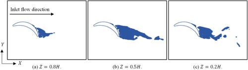
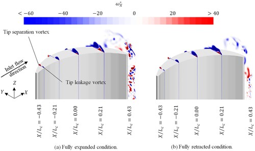
As can be seen in Figure 17, there are significant vortices induced by the tip of the rigid wingsail. By plotting ${\omega }_X^{\ast }$ at several different streamwise positions around the tip (Figure 19), two tip vortices, the tip separation vortex and the tip leakage vortex, can be found developing at the suction side and the pressure side, respectively. According to the uRANS simulations as well as previous studies (Zhu et al. 2022), the two vortices combine at around the half chord into a single vortex with a more complex internal flow structure. Nevertheless, in the IDDES results, the two vortices do not combine. The tip leakage vortex is much stronger than the tip separation vortex, which dissipates quickly at around the half chord. Due to the higher apparent wind speed, the tip vortices are stronger under the fully retracted condition. However, when comparing the dimensionless value of ${\omega }_X$, the distribution is quite similar between the two conditions.

Figure 19. Non-dimensional ${\omega }_X$ distribution at different streamwise positions around the tip, based on the IDDES simulations, $\alpha ={23}^{\circ }$. For the fully expanded condition, $V_{AW}=8\mathrm{m}/\mathrm{s}$, while for the fully retracted condition, $V_{AW}=32\mathrm{m}/\mathrm{s}$. This figure is available in colour online.

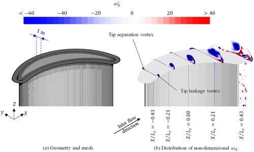
A disc plate, which extends $1\mathrm{m}$ from the boundary of the top section and is $0.1\mathrm{m}$ in thickness, is installed upon the top of the sail, as Figure 20(a) shows. An extra CFD simulation based on IDDES method is performed to study the effect of this disc plate. In this case, $\alpha$ is ${23}^{\circ }$, and the physical condition is the fully expanded condition. By having this disc plate, $C_L$ increases around $1\text{\%}$. When looking at the ${\omega }_X$ distribution in Figure 20(b), the tip separation vortex developing on the suction side almost disappears; however, the tip leakage vortex developing on the pressure side is still quite strong. This could be because the scale of the tip leakage vortex is around $1.5\mathrm{m}$, which is larger than the extension of the disc plate from the sail. A previous study compared the CFD results of a crescent-shaped wingsail with and without a freestream tip (Zhu et al. 2022), indicating that the loss of $C_L$ due to the freestream tip is about $6\text{\%}$. Therefore, the shape of the tip can still be further optimised to obtain a higher $C_L$.

Figure 20. Geometry, mesh, and effects of the disc on top based on IDDES simulations, fully expanded condition, $V_{AW}=8\mathrm{m}/\mathrm{s}$, $\alpha ={23}^{\circ }$. This figure is available in colour online.

4. Conclusions

This study aimed to develop an improved high-fidelity CFD model for rigid wingsails with crescent-shaped sectional profiles. The improved model not only predicts the propulsive performance, but also unveils the high-frequency and wake characteristics of the flow field, which are important for further FSI and multiple-sail studies. The telescopic function of the wingsails was also studied, for a range of different angles of attack, by comparing the propulsive performance under the fully expanded and the fully retracted conditions. The computational methods used were uRANS and IDDES with the $k-\omega$ SST turbulence model. The flow separation, vortex shedding in the wake region, and tip vortices were analysed. The outcome of the study provides guidance for further studies on structural analysis, FSI analysis, multi-sail interaction analysis, and profile optimisation of telescopic wingsails.

For the time-averaged force coefficients, which are the primary determinants of propulsive performance, uRANS and IDDES had a similar prediction. The maximum $C_L$ was obtained when $\alpha$ was ${23}^{\circ }$. For the fully expanded condition, the lift and drag coefficients based on the IDDES results were $2.102$ and $0.456$, respectively, while when the sail was fully retracted, $C_L$ and $C_D$ changed by $-8.9\text{\%}$ and $17.1\text{\%}$. Therefore, wingsails with a crescent-shaped profile can achieve significant propulsive performance.

However, the external loads predicted by the two methods show different unsteady characteristics, which are believed to have a non-negligible influence on the structural response. From the FFT analysis, the results based on uRANS showed clearer low-frequency oscillations than those based on IDDES, while the IDDES results showed some high-frequency characteristics of the external loads. The high-frequency oscillations may lead to local vibration or buckling of the structures, which could be studied in a future FSI analysis. This difference is likely because the IDDES method can provide more detailed information about the flow field, especially the vortex shedding in the wake region, because large-scale eddies are solved without modelling. In addition, due to the oscillation of the wind loads, studies on the structural response are necessary to avoid structural failures such as plastic deformation, buckling, and fatigue. For analyzing the structural response, especially the local vibration of the structure, LES or DES-typed methods are necessary.

Vortex tubes extending in the spanwise direction could be detected in the uRANS results, but the structure of the vortex is quite complex in the IDDES results. The IDDES method also indicated less dissipation and energy loss in the wake region, due to which vortex structures could be clearly seen $42\mathrm{m}$ (3 times the chord length) downstream of the sail. It can be inferred that the wake flow can cause interactions among sails on a ship with multiple sails.

Meanwhile, the negative effects on the propulsive performance due to tip vortices are significant, especially when the sail is retracted. Having a disc plate on the top of the sail can increase $C_L$ by $1\text{\%}$, but further optimisation of the tip geometry should be studied in the future.

Disclosure statement

No potential conflict of interest was reported by the author(s).

Data availability statement

The data that support the findings of this study are available from the corresponding author, Heng Zhu, upon reasonable request.

Nomenclature
$C_D$	=	Drag force coefficient [-]
$C_L$	=	Lift force coefficient [-]
$C_M$	=	Moment coefficient [-]
$C_p$	=	Pressure coefficient [-]
$C_T$	=	Thrust force coefficient [-]
$C_{T,max}$	=	Maximum thrust force coefficient [-]
$E$	=	Young’s modulus [$\mathrm{G}\mathrm{P}\mathrm{a}$]
$H$	=	Sail height (spanwise length) [$\mathrm{m}$]
$L_c$	=	Chord length [$\mathrm{m}$]
$P$	=	Pressure [$\mathrm{P}\mathrm{a}$]
$Q$	=	Q-criterion [${\mathrm{s}}^{-2}$]
$Re$	=	Reynolds number [-]
$V_{AW}$	=	Apparent wind speed (inlet velocity) [$\mathrm{m}/\mathrm{s}$]
$V_S$	=	Ship speed [$\mathrm{m}/\mathrm{s}$]
$V_{TW}$	=	True wind speed [$\mathrm{m}/\mathrm{s}$]
$V_X$	=	Streamwise velocity [$\mathrm{m}/\mathrm{s}$]
$w$	=	Deformation displacement [$\mathrm{m}$]
$y^{+}$	=	Dimensionless wall-normal distance [-]
$\alpha$	=	Angle of attack [${}^{\circ }$]
${\alpha }_c$	=	Critical angle of attack [${}^{\circ }$]
${\theta }_{AW}$	=	Apparent wind angle [${}^{\circ }$]
${\theta }_{TW}$	=	True wind angle [${}^{\circ }$]
$\mu$	=	Dynamic viscosity [$\mathrm{P}\mathrm{a}\cdot \mathrm{s}$]
$\rho$	=	Air density [$\mathrm{k}\mathrm{g}/{\mathrm{m}}^3$]
${\rho }_{\mathrm{A}\mathrm{l}}$	=	Aluminum density [$\mathrm{k}\mathrm{g}/{\mathrm{m}}^3$]
$\nu$	=	Poisson’s ratio [-]
${\sigma }_{yield}$	=	Yield stress [$\mathrm{M}\mathrm{P}\mathrm{a}$]
${\omega }_X$	=	Streamwise vorticity [${\mathrm{s}}^{-1}$]
${\omega }_X^{\ast }$	=	Non-dimensional streamwise vorticity [-]
${\omega }_Z$	=	Spanwise vorticity [${\mathrm{s}}^{-1}$]
${\omega }_Z^{\ast }$	=	Non-dimensional spanwise vorticity [-]

Additional information

Funding

This work was performed within the project WindStruc (Wind-assisted propulsion for commercial vessels) funded by the Swedish Energy Agency through contract agreement no. 51552-1, co-funded by ScandiNAOS AB and Stena Rederi AB. During the process of this study, Bengt Ramne from ScandiNAOS AB put forward the concept design of the sail, and Carl-Erik Janson from Chalmers University of Technology also offered guidance supporting the CFD simulations and propulsive analysis. The computations and data handling were enabled by resources provided by the Swedish National Infrastructure for Computing (SNIC), partially funded by the Swedish Research Council through grant agreement no. 2018-05973.

References

- ASTM. 2004. Standards specification for aluminum and aluminum-alloy sheet and plate. Philadelphia, USA: American Society for Testing and Materials.
- Atkinson GM. 2019. Analysis of lift, drag and CX polar graph for a 3D segment rigid sail using CFD analysis. J Mar Eng Technol. 18(1):36–45. doi: 10.1080/20464177.2018.1494953.
- Blount H, Portell JM. 2021. CFD investigation of wind powered ships under extreme conditions. Gothenburg, Sweden. https://odr.chalmers.se/handle/20.500.12380/304254.
- Dassault Systemes. 2020. Abaqus analysis user's guide.
- Davidson L. 2019. Fluid mechanics, turbulent flow and turbulence modeling. Gothenburg, Sweden: Division of Fluid Dynamics, Department of Mechanics and Maritime Sciences, Chalmers University of Technology.
- EUROSTAT. 2019. Greenhouse gas emissions by source sector. Luxembourg, Luxembourg: EUROSTAT.
- Hamada N. 1985. The development in Japan of modern sail-assisted ships for energy conservation. Regional Conference on Sail-motor Propulsion, Manila, Philippines.
- Hilsenrath J. 1955. Tables of thermal properties of gases: comprising tables of thermodynamic and transport properties of air, argon, carbon dioxide, carbon monoxide, hydrogen, nitrogen, oxygen, and steam. Vol. 564. Gaithersburg, USA: US Department of Commerce, National Bureau of Standards.
- IMO. 2018. Interpretation of initial IMO strategy on reduction of GHG emissions from ships. Vol. 60, p. 195–201.
- International Chamber of Shipping. 2014. Shipping, world trade and the reduction of CO2 emissions. London: International Chamber of Shipping.
- International Transport Forum. 2020. Navigating towards cleaner maritime shipping. OECD Publishing. www.itf-oecd.org.
- Khan L, Macklin J, Peck B, Morton O, Souppez J-BRG. 2021. A review of wind-assisted ship propulsion for sustainable commercial shipping: latest developments and future stakes. Proceedings of the Wind Propulsion Conference 2021, London, UK.
- Kimball J. 2009. Physics of sailing. CRC Press. doi: 10.1201/9781420073775.
- Lee H, Jo Y, Lee DJ, Choi S. 2016. Surrogate model based design optimization of multiple wing sails considering flow interaction effect. Ocean Eng. 121:422–436. doi: 10.1016/j.oceaneng.2016.05.051.
- Lu R, Ringsberg JW. 2020. Ship energy performance study of three wind-assisted ship propulsion technologies including a parametric study of the Flettner rotor technology. Ships Offsh Struct. 15(3):249–258. doi: 10.1080/17445302.2019.1612544.
- Ma Y, Bi H, Gan R, Li X, Yan X. 2018. New insights into airfoil sail selection for sail-assisted vessel with computational fluid dynamics simulation. Adv Mech Eng. 10(4):168781401877125. doi: 10.1177/1687814018771254.
- Menter FR. 1993. Zonal two equation κ-ω turbulence models for aerodynamic flows. AIAA 23rd Fluid Dynamics, Plasmadynamics, and Lasers Conference, Orlando, FL, USA.
- Nikmanesh M. 2021. Sailing performance analysis using CFD simulations: a study on crescent shaped wing profiles. https://odr.chalmers.se/handle/20.500.12380/304303.
- Patankar SV. 1981. Numerical heat transfer and fluid flow. CRC Press. doi: 10.13182/nse81-a20112.
- Rousmaniere J. 1999. The annapolis book of seamanship:: completely revised, expanded and updated. New York, USA: Simon and Schuster.
- Sauzé C, Neal M. 2008. Design considerations for sailing robots performing long term autonomous oceanography. Proceedings of the International Robotic Sailing Conference. 27(2). p. 21–29. www.roboticsailing.org.
- Shur ML, Spalart PR, Strelets MK, Travin AK. 2008. A hybrid RANS-LES approach with delayed-DES and wall-modelled LES capabilities. Int J Heat Fluid Flow. 29(6):1638–1649. doi: 10.1016/j.ijheatfluidflow.2008.07.001.
- Siemens PLM Software. 2021. STAR-CCM+ user guide (version 16.02). Munich, Germany: Siemens PLM Software Inc.
- Silva MF, Friebe A, Malheiro B, Guedes P, Ferreira P, Waller M. 2019. Rigid wing sailboats: a state of the art survey. Ocean Eng. 187:106150–106150. doi: 10.1016/j.oceaneng.2019.106150.
- Smagorinsky J. 1963. General circulation experiments with the primitive equations. Mon Weather Rev. 91(3):99–164. doi: 10.1175/1520-0493(1963)091<0099:GCEWTP>2.3.CO;2.
- Tillig F, Ringsberg JW. 2020. Design, operation and analysis of wind-assisted cargo ships. Ocean Eng. 211:107603–107603. doi: 10.1016/j.oceaneng.2020.107603.
- Traut M, Gilbert P, Walsh C, Bows A, Filippone A, Stansby P, Wood R. 2014. Propulsive power contribution of a kite and a Flettner rotor on selected shipping routes. Appl Energy. 113:362–372. doi: 10.1016/j.apenergy.2013.07.026.
- Workinn D. 2021. A high-level interface for a sailing vessel. http://urn.kb.se/resolve?urn=urn:nbn:se:kth:diva-299430.
- Zhu H, Nikmanesh MB, Yao HD, Ramne B, Ringsberg JW. 2022. Propulsive performance of a novel crescent-shaped wind sail analyzed with unsteady rans. Proceedings of the International Conference on Offshore Mechanics and Arctic Engineering – OMAE, Hamburg, German.