Mapping the annual evolution of snow depth in a small catchment in the Pyrenees using the long-range terrestrial laser scanning

Abstract

This paper presents the methodology used to develop snow depth distribution maps for a small catchment in the Central Spanish Pyrenees covering 55 ha in a 1:10,000 scale. The Main Map was obtained using LiDAR (light detection and ranging) technology from a long-range Terrestrial Laser Scanner (TLS) in six field surveys undertaken during the 2012 winter–spring period. This technique enabled the acquisition of information at a very high resolution concerning the spatial variability of snow cover, providing snow depth information for remote areas where data acquisition is complex and hazardous. We describe the methodological steps and the quality assessment applied in developing the maps. Comparison with manual measurements confirmed the reliability of the snow depth maps, including areas located at large distances from the scanner (800 m). This method provides a promising tool for future investigations of snow dynamics in mountainous environments.

Keywords:

• snow depth distribution maps
• terrestrial laser scanner
• Pyrenees
• application protocol

1. Introduction

In mountainous areas the snowpack has very high spatial variability as a consequence of vertical lapse rates in temperature (which affect the phases of precipitation), the distribution of precipitation amounts, terrain shadows caused by complex topography, ground irregularities, and snow redistribution by wind and avalanches (Deems, Fassnacht, & Elder, 2006; Grünewald, Schirmer, Mott, & Lehning, 2010; Liston & Sturm, 2002; López-Moreno, Fassnacht, Beguería, & Latron, 2011). Accurate maps of snow duration and thickness provide valuable information for understanding many environmental processes that occur in mountainous areas, including the distribution and survival rates of plants (Keller, Kienast, & Beniston, 2000; Körner, 1994), soil temperature and moisture (Groffman et al., 2001; Gross, Hardisky, Doolittle, & Klemas, 1990), identification of avalanche start and runout zones (Birkeland, Hansen, & Brown, 1995; Sovilla, 2004), erosion rates (Colbeck et al., 1979; Pomeroy andray, 1995), and runoff dynamics and snow cover depletion in mountainous catchments (Lehning et al., 2006; Pomeroy, Essery, & Toth, 2004), among many other factors.

The importance of snow has focused scientific interest during the last two decades on the mapping of snow depth (SD) and the snow water equivalent (SWE) at various spatio-temporal scales (Bales & Harrington, 1995; Erickson, Williams, & Winstral, 2005). A widely used mapping procedure is focused on estimating SD and the SWE as a function of terrain characteristics. In this approach various topographic and geographic features, generally derived from a digital elevation model (DEM), are used as predictor variables on the basis that they are closely related to the accumulation, redistribution, and ablation of snow cover (Bavera & De Michele, 2009; Erxleben, Elder, & Davis, 2002; Jost, Weiler, Gluns, & Alila, 2007; Molotch, Colee, Bales, & Dozier, 2005). When the relations between snow accumulation and predictor variables have been established, the spatial distribution of SD can be determined for areas with well-known terrain characteristics. This technique is one of the so-called regression-based methods. It requires the acquisition of many SD or SWE measurements in complex and often dangerous terrain, and is subject to several uncertainties regarding the effects of grid and sample size (digital terrain model resolution and number of data points respectively) (López-Moreno, Latron, & Lehmann, 2010).

As manual high-resolution SD data acquisition over large areas is unfeasible, remote sensing techniques have recently been applied for this purpose. Examples include LiDAR (light detection and ranging) techniques, which commonly utilize airborne or terrestrial laser scanners (respectively ALS and TLS). In recent years these have provided accurate results in SD studies compared with other techniques (Deems et al., 2006; Hopkinson, Chasmer, Young-Pow, & Treitz, 2004; Jörg, Fromm, Sailer, & Schaffhauser, 2006; Prokop, Schirmer, Rub, Lehning, & Stocker, 2008; Schaffhauser et al., 2008). For medium-sized and small areas the TLS technique (Lundberg, Gustafsson, & Granlund, 2008) represents a more flexible and inexpensive option as compared to ALS, as TLSs are portable and snow can be surveyed without using an aircraft (note the costs of hiring an aircraft). In addition, SD can be sampled at the most suitable spatial resolution for the useŕs needs. Although the application of TLSs is not currently widespread in Alpine areas, an increasing number of studies have highlighted its accuracy and usefulness for snow studies in which high-resolution data are required (Egli, Jonas, Grünewald, Schirmer, & Burlando, 2012; Grünewald et al., 2010; Prokop, 2008).

In this study a long-range TLS was used to obtain high spatial resolution snow cover and depth distribution maps in a small mountain catchment (55 ha) in the Central Spanish Pyrenees. We describe the protocol followed for generating snow distribution maps during the snow accumulation and melting periods in 2012. To assess the robustness of this protocol, the data obtained at various distances from the TLS were compared with direct manual SD measurements.

2. Study area

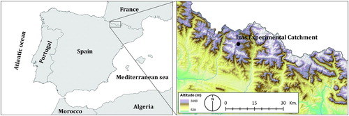
The Izas experimental catchment has an area of approximately 55 ha and is located in the central Spanish Pyrenees (42°44′ N, 0°25′ W) between 2000 and 2300 m above sea level (asl). This area is close to the main divide of the Pyrenees in the headwaters of the Gállego River, near the border with France (Figure 1). The catchment is exposed to Atlantic climate conditions, and consequently the winters are relatively humid, and the snowpack covers most of the catchment from November to the end of May (López-Moreno et al., 2010). The winter and spring of 2012 were particularly dry and mild, and the snowpack remained below the average throughout the winter and into the spring. However, late snowfall events by the end of April increased the amount of snow at the end of the melting period. The vegetation cover is composed of high mountain pastures, although in some areas the ground is bare of vegetation, with rocky outcrops occurring in steeper areas (less than 15% of the study area). The mean slope of the catchment is 16° (López-Moreno, Pomeroy, Revuelto, & Vicente-Serrano, 2012).

Figure 1. The study area showing the location of the Izas experimental catchment. The left panel represents the geographical location in the Iberian Peninsula, and the right panel depicts a zoomed image of the Central Spanish Pyrenees.

3. Terrestrial laser scanner

LiDAR are those remote sensing technologies that emit laser light, and measures the distance between the target and the device based on the phase shifting of light, time of flight measurement or interferometry. LiDAR technology has undergone rapid development in recent years and both, terrestrial and airborne LiDAR have been used in several types of geomorphological studies, including those investigating rock falls (Abellán, Vilaplana, & Martínez, 2006; Abellán, Calvet, Vilaplana, & Blanchard, 2010), landslides (Bitelli, Dubbini, & Zanutta, 2004; Jaboyedoff et al., 2012; Oppikofer, Jaboyedoff, & Keusen, 2008), fluvial dynamics (Heritage andetherington, 2007) and soil degradation (Romanescu, Venedict, Cotiuga, & Asandulesei, 2011).

The device used in the present study is a long-range TLS (RIEGL LPM-321), which uses time of flight technology. The device measures the time between a light pulse emission and its detection. The resulting value is multiplied by the speed of light through air, and divided by two (the measured time is twice the time required for the light pulse to reach the target from the TLS; Figure 2). Each distance measurement is repeated for every single point acquired in the area of interest, obtaining a three-dimensional point cloud from real topography.

Figure 2. Time of flight technology and footprint characteristics of the LPM-321 TLS. This is a simplified figure with footprint perspective for different distances and incident angles, where d_i are distances [m], t is time of flight [s], c is light speed propagation [m/s], δ is laser beam divergence [°], α is incidence angle between the surface normal and laser beam direction [°], and F_i are footprint sizes [m²]. In the upper panel of the figure two footprints for the same distance are represented with different incidence angles, showing the increase in footprint size when incidence angle increases. In the main panel, two footprints with a normal incidence angle between surface and laser beam direction for two distances, show the increase of footprint size with distance.

The technical characteristics of the TLS used are: (a) light pulses of 905 nm wavelength (near-infrared), which is ideal for acquiring data from snow cover (Prokop, 2008); (b) minimum angular step width of 0.018°; (c) laser beam divergence of 0.046°; and (d) maximum working distance of 6000 m. The sampling speed depends on the operation mode, which in turn depends on the target distance, but ranges from 10 to 1000 Hz; this enables large areas to be surveyed in a reasonable time. This TLS has been shown to be an appropriate tool for deriving high-resolution DEMs applicable to cryosphere studies (Avian & Bauer, 2006; Egli et al., 2012; Grünewald et al., 2010; Schwalbe, Mass, Dietrichb, & Ewert, 2008).

Despite the number of recent studies in which TLSs have been used, the technique is still considered novel, with a limited number of applications to snow studies. When used for scanning at large distances, various error sources need to be taken into account and minimized (Reshetyuk, 2006). Thus, it is important to establish a protocol for obtaining data and generating accurate DEMs that will facilitate development of accurate SD distribution maps. This paper describes the operational procedure used for generating those maps for the Izas experimental catchment in the Central Spanish Pyrenees.

4. Data collection

In this section the methodological steps applied for collecting data are fully explained, first a short introduction of the experimental setup is presented, followed by the scanning procedure applied for each survey.

4.1. Experimental setup design

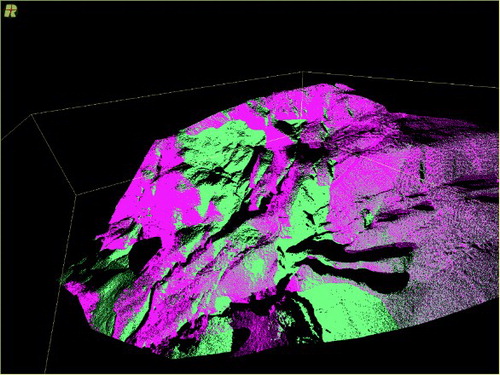
The first step, which precedes data collection with the TLS, is to consider several factors for choosing the optimal position (or positions) to place the TLS (scan station). LiDAR is a line-of-sight technique (i.e., any object placed between the TLS and the study area will prevent the acquisition of information behind it) where the cost of multiple scan stations should be weighed against the benefit (i.e., occlusion reduction). As the Izas Experimental Catchment presents a relatively smooth topography with a single scan station 62% of the area is covered (scan station 1 in Figure 3), but the south zone of the study area is hidden from this point of view. Consequently, a second scan station, placed by around 450 m away from scan station 1, was established in the central area of the catchment (see scan station 2 in Figure 3). This enabled the reduction of topographic shadows in the final points cloud as is shown in Figure 4 and therefore 86% of the study area was scan covered in final maps. Furthermore, carrying the TLS equipment and accessories (e.g., tripod, batteries, laptop and cables), with a weight of around 45 kg, in alpine terrain with snow presence, must be considered. Thus, experimental area and scan stations should be chosen properly to accommodate logistical considerations.

Figure 3. Digital elevation model of the Izas Experimental Catchment showing the locations of the two scan stations (1 and 2) and the 12 target used in this study. The locations of plots where manual SD measurements were taken are showed.

Figure 4. Point cloud with topographic shadows. This is a perspective view from the three- dimensional data. The magenta color shows areas visible from scan station 1, and cyan shows areas visible from the scan station 2. Areas with points of both colors (magenta and cyan) are visible from both scan stations. The black shading shows areas in which no measurements were possible.

Indirect registration, also called target-based registration, was used to merge the information from the different scan stations, and for transforming the local coordinates of the obtained point clouds into a global coordinate system. It enabled the comparison of scans made on different survey days. Indirect registration uses fixed reference points (targets) that are located in the study area. Those targets must be visible to all scan stations because they are used for transforming coordinates, as described in the next section. Reflective targets of known shape and dimensions are placed at those reference points. Although a minimum of three targets should be used, we installed 12 within the experimental basin, each comprising a cylindrical reflector 0.25 m high × 0.25 m diameter mounted on a pole 2 m tall (Figure 3). The distance of the targets to the two scan stations ranged from 110 to 730 m. This number of targets increased the robustness of the experimental setup and prevented any target loss. Using standard topographic methods we obtained accurate global coordinates for the targets using a differential global positioning system (GPS) with post-processing and a total station. Two GPS base-station receivers with a long measuring time (up to 2 h) should be established in the study area (note that all targets should be visible from at least one of them to undertake afterwards an optical survey), and their positions corrected using data from a permanent GPS station. When both bases were correctly established and marked, a total station was positioned at the base where all targets were visible, and orientated towards the second base. The global coordinates of the targets were acquired using this total station undertaking an optical survey. In our study the global coordinates were acquired in the UTM 30 coordinate system in the ETRS89 datum. The final precision for the global target coordinate was 0.05 m by planimetry and 0.1 m by altimetry.

4.2. Scanning procedure

In order to reduce one of the most important error sources related with the equipment stability, some considerations about assembling and positioning the TLS must be taken into account. The TLS is mounted using a tribrach (for leveling the device) on a topographic tripod. The equipment must be properly assembled and stabilized to avoid any disturbance (e.g. vibration) to the scanner position, which can introduce considerable errors in measurements made over large distances; for example, a deviation of 8′ produces a deviation of 2.32 m at a distance of 1000 m. This issue is particularly relevant in snow-covered areas, where the weight of the TLS device and the vibration produced during the scanning process can cause movement if the tripod is placed on snow or frozen surfaces. Hence, it is strongly recommended to: (1) mount the tripod on bare rock surfaces; (2) compact the snow around the tripod; or (3) build stable platforms (e.g. concrete surfaces) where possible.

The last stage before acquiring the point cloud of the study area is the registration of the scan station. This step includes the atmospheric correction and the scan of the targets. Light pulses propagate through the air, with the speed of propagation depends on the air refraction index, which is dependent on atmospheric pressure and air temperature and humidity. For this reason an atmospheric correction is needed. When the equipment is assembled, these three atmospheric variables are measured using a digital thermohygrometer and a barometer; these measurements are used by the software that controls the TLS (Riprofile) to correct the light speed propagation value (Ullrich, 2005). Using this correction, light speed in the air can be inferred and the distance to each point accurately obtained by the TLS. After atmospheric correction, the 12 targets of the study area are scanned to provide the reference point coordinates that will be used for the indirect registration. In this study, atmospheric correction and target coordinates acquisition were repeated at 1 or 1.5 hour intervals. The porpoise of this, is to detect instability problems, and atmospheric or snow surface changes. This time interval is consistent with the recommendation of repeating both operations at intervals of less than two hours (Prokop, 2008).

Once all the above mentioned steps have been completed, the scan of the study area can be started. First, the area of interest is selected and the TLS is aimed at the two opposite corners of the area to be scanned. In this way a rectangular area is chosen, in which a virtual spatial matrix having the desired resolution is generated. Several factors should be considered when selecting the appropriate spatial resolution. The TLS works on polar coordinates, and automatically transforms the acquired point coordinates to the Cartesian coordinate system. It is important to differentiate between angular and linear resolution. While angular resolution remains constant, linear resolution will change depending on distance to the TLS. Thus, the greatest and least distances in the selected area should be measured (using the TLS), and averaged to estimate the middle distance. Following this the angular resolution is calculated for the desired linear resolution, and this angular resolution is used for selecting the angular step width for the scan. As the working frequency of the TLS depends on the operational mode, which is dependent on distance, the acquisition speed depends on the average distance between the TLS and the selected area. As the scanning duration is limited, a compromise between resolution, operational mode and the area to be scanned is needed.

In this study, the average resolution in point cloud acquisition (spacing between points) was 0.35 m, with resolutions between 0.1 m (areas nearest to the TLS) and 0.6 m (areas furthest from the TLS). To achieve those values, the angular scanning resolution has been selected depending on the range between the scanned surface and the TLS, as it is presented in Table 1. In the TLS literature, the standardized unit for measuring point cloud density is points per square meter, which results more useful for considering the cell size value of the DTM that will be generated for each survey. For a normal incidence angle with the scanned surface (0° between laser beam direction and the surface normal vector, see upper panel of Figure 2) the number of points/m² is at a maximum; but if this angle increases, the number of points/m² is reduced as shown in Table 1. This study presents a final cell size value of 1m, and therefore the number of points/m² can be directly related to Table 1 values. From this table, it is clear that only for the highest incidence angles at large distances (75° at 1000 m), the points cloud density is inadequate (lower than 1 point/m²), which occurs in a negligible area of the catchment. To summarize, the average number of points scanned in each survey was around 4 million. Moreover, in order to scan the entire study area, respecting the time interval of 1.5 hours in target acquisition and atmospheric correction, between six and eight scans (from both scan stations) were undertaken.

Table 1. Angular resolutions, linear resolutions, and the density of the obtained point cloud at different distances from the TLS.

			Points/m^2 for different incidence angles (α)
Range (m)	Angular Resolution (°)	Linear Resolution (m)	0°	15°	30°	60°	75°
1000	0.036	0.63	2.5	2.4	2.2	1.3	0.9
900	0.036	0.57	3.1	3.0	2.7	1.6	1.1
800	0.036	0.50	4.0	3.8	3.4	2.0	1.4
600	0.036	0.38	7.0	6.8	6.1	3.5	2.4
^a600	0.064	0.67	2.2	2.2	1.9	1.1	0.8
400	0.064	0.45	5.0	4.8	4.3	2.5	1.7
200	0.064	0.22	20.0	19.4	17.4	10.0	6.9
^a200	0.11	0.38	6.8	6.6	5.9	3.4	2.3
100	0.11	0.19	27.1	26.2	23.5	13.6	9.3
50	0.11	0.10	108.5	104.8	94.0	54.3	37.1

^aNote that values for the 200 m and 600 m ranges are duplicated, because the 200 m range is normally the limit for using near or medium range, and 600 m range is the limit for using medium or long range.

It is important to consider the beam width, because the laser beam divergence (0.8 mrad = 0.046°) leads to an elliptical footprint for what is considered to be a single point (Figure 2). This means that each point is the average distance to several points of real topography with the calculation depending on the operational mode of the TLS. As the object distance increases so does the footprint, but distance is not the only variable affecting footprint area. When the incidence angle between the laser beam direction, and the normal vector of the scanned surface increases, the footprint area also increases (upper panel in Figure 2). For instance, for a distance of 200 m and an incidence angle of 0°, the footprint area is 0.02 m², increasing to 0.11 m² with an incidence angle of 80°; for these angles (respectively), these areas increase to 0.5 m² and 2.9 m² for a distance of 1000 m, and 8 m² and 46 m² for a distance of 4000 m (Prokop, 2009). The relationship between incidence angle and terrain reflectivity affects pulse intensity reflection (Wagner, Ullrich, Melzer, Breise, & Kraus, 2004); the varying behavior of the signal return therefore depends on terrain properties. Another consideration in beam divergence occurs when the maximum resolution (0.018°, the minimum angular step width) is selected, as adjacent footprints may overlap. However, it has been established that the optimal overlap of footprints is 85% of laser beam divergence (Lichti & Jamtsho, 2006) and the TLS used in this study satisfies this overlapping optimum. Nevertheless, recent studies have suggested that footprint increases at high incidence angles has a negligible effect on the quality of the final point cloud (Schürch, Densmore, Rosser, Lim, & McArdell, 2011).Therefore it is an effect that must be considered but it is not a limiting factor of the data quality.

The emission spectrum of the sun includes near infrared wavelengths. Thus, if there is sunlight reaching the scanned area, or sunlight impacts directly on the TLS receptor, the signal–noise ratio could affect signal detection (Wehr & Lohr, 1999). If this effect is combined with high incident angles on wet snow surfaces (angles > 30°), no signal is detected by the TLS detector (Prokop, 2008). Furthermore, with scanning at large distances (>1000 m) some acquisition points are lost because of the combination of sunlight and large incident angles. It has been observed that this problem is largely avoided when no sunlight affects the scan, so for areas with signal detection problems (long range and large incident angles) the scan must be performed in the absence of sunlight (at sunset or during the night). At this point, it is interesting to note that no effect on signal detection has been observed with the different snow albedos given during the snow season. Finally, for optimal results the TLS should not be operated during unstable weather conditions (e.g. cloudy, rainy or windy days), because of erroneous points being acquired during precipitation, destabilization of the system by wind, and the absorption of near infrared wavelengths by clouds.

When a scan has been completed, pictures are acquired using a digital camera coupled to the TLS. Images are useful for obtaining RGB (red/green/blue) information for each point, which can be used for further analysis and verification. For example, this information is useful to account SD errors in the limits of snow patches (not presented in this paper).

5. Data processing

Several studies have highlighted the importance of choosing an appropriate georeferencing procedure (Williams, 2012), and the need to establish a rigid geodetic network for reducing misalignments and systematic errors (Rub, 2007). For georeferencing data we used an indirect procedure, named indirect registration, that uses reference point coordinates (Reshetyuk, 2006) where targets are located. The point clouds obtained are recorded in the relative coordinate system of the TLS (SOCS). Thus, targets enable the transformation of coordinates for each point cloud into a project coordinate system (PRCS) common for all scan stations of a single survey. Subsequently, transformation of the point cloud into a global coordinate system (GLCS) is needed to generate a georeferenced DEM.

Based on the coordinates of the targets a transformation matrix (translation and rotation matrix) is generated (using Riprofile® software), which may merge point clouds from the different scan stations and the SOCS coordinate transformation to PRCS, and finally to GLCS. Each matrix calculation is associated with a standard deviation calculation that provides information about the error in target coordinate acquisition for all registration processes during the survey project. This error increases with distance. In this study we found that the standard deviation was approximately 0.008 m, which increased to 0.03 m when the global coordinates of the target were included (note that errors in global coordinate acquisition increase the standard deviation). This standard deviation is adequate for the study purpose, because with this value, errors originating in the point cloud registration are below the SD differences, even at large distances (for example, at 730 m, the furthest target from scan stations, the average altitudinal error of its location is 0.023 m).

From the obtained point clouds for every survey day, a DTM is derived. Given the high density of points in our study area and the relatively smooth topography of the catchment, point data were directly rasterized at a grid size resolution of 1 m². In this manner, for every single survey, the elevations of all points within each raster cell were averaged. The cells with no point information were discarded and assigned as ‘no data’. Raster masks were created to avoid erroneous calculations for areas in shadow.

Finally, each SD map was obtained by subtracting the snow free catchment DTM (scanned in July) from each DTM created for the six survey days from mid-February to the end May. This is the last product obtained out of the presented methodology.

6. Data analysis

The SD maps obtained for each date are presented in the main map. The distribution of the snowpack reveals the high variability of snow, even over very short distances. For example, in periods of very little snow accumulation (as occurred in winter–spring 2011–2012) there are concavities in the terrain that accumulate more than 5 m of snow depth, and at short distances, the SD could be reduced to less than 1 m. In addition, it is clearly observed how in those concavities the snow lasts until the end of the melting period. Qualitatively, this evolution can be seen in the snow distribution maps for 2 May 2012 (obtained from measurements made immediately following an accumulation event) and the two subsequent surveys (14 and 24 May 2012), made when meteorological conditions led to rapid snow melt. Thus, if the snowpack evolution is monitored during the snow season, it is clear that SD maps represent a powerful database for studying snow cover variability and also for studying snow accumulation and fusion patterns, relating the obtained maps with topographic variables, and meteorological data, if these are available.

Many authors have analyzed the uncertainty in data derived from TLS in relation to (1) errors in point cloud acquisition (Abellán, Jaboyedoff, Oppikofer, & Vilaplana, 2009; Hodge, Brasington, & Richards, 2009) and (2) in DTM generation (Lane, Westaway, & Murray Hicks, 2003; Wheaton, Brasington, Darby, & Sear, 2010). More recently Schürch et al. (2011), concluded that the elevation ambiguity in points within the same raster cell obtained from different scan stations, is principally originated from errors of point cloud registration and surface roughness. Despite the differences in scale with other studies and the particularities of the Izas Experimental Catchment, those studies highlight the importance of establishing an appropriate experimental setup and following a well-established procedure for minimizing error sources as is presented here. Considering Schürch et al. (2011), elevation ambiguities could be related with errors from point cloud registration and surface roughness. In this study, instead of considering this numerical analysis of errors in the DTM generation; the altitudinal differences in raster cells for the base DTM (i.e., snow free) and the obtained DTMs snow-covered, are compared to direct measurements of snow depth, which represents a good option to consider errors of final SD maps.

In order to evaluate the quality and the accuracy of the obtained snow maps from TLS, manual SD measurements were made during each survey. However, it was not possible to directly relate the locations of manual measurements (determined using a hand-held GPS (Garmin GPSmap 60CSx), which had an estimated error of ±5 m) to those of scanned measurements, where the acceptable error should not exceed a few tens of centimeters. Moreover, site-specific SD acquisition should take into account that high snow variability occurs over short distances and is affected by topographic irregularities at very small scales (decimeters; e.g. the presence of rocks, bushes and other terrain features).

For these reasons three ‘validation’ plots were defined in the catchment, having average distances from the TLS of 200 m, 400 m and 800 m. The plots were 20 × 20 m and included flat, concave and convex areas. The SD in these plots was measured using a 5-m long anodized aluminum snow probe in a 2 × 2 m grid. Using this approach it was possible to assess whether information obtained using the TLS accurately represented the mean and variability of the snowpack depth at the plot scale, and also enabled assessment of whether distance to the scan position affected the accuracy of the acquired data. López-Moreno et al. (2011) used an extensive dataset of manually measured snow variability to demonstrate that using only eight SD measurements in a plot of 10 × 10 meters was enough to drastically reduce the error when estimating the measured average ground truth and the variance at the plot scale (below 5% in 75% of analyzed cases). Similar conclusions can be derived from the study of Fassnacht and Deems (2006) who compared different resolution and resampling methods to quantify local snow variability and scale breaks. These results suggest that the different resolutions of manual (2 meters) and TLS snow measurements (1 meter) should not affect seriously the comparison of average snow depth estimation and its variability in the validation plots.

The non-parametric Whitney-Wilcoxon statistical test (Siegel & Castelan, 1988) was used to determine the possible statistically significant differences between SD measured manually and from TLS at a significance level of 0.05. Differences between SD measured manually and from TLS were not statistically different in more than 80% of the cases, with only three exceptions: for medium range the 2 April 2012 and 17 April 2012, and for long range the 14 May 2012 (marked with * in Figure 5), so it is reasonable to compare TLS and manual measurements, as these do not show differences (at a significance threshold of 95%). Figure 5 shows box plots representing the mean and variability of the snowpack measured using the manual snow probe, and the values of the TLS-based gridded maps measured on each surveyed day. Accurate snowpack quantification was achieved at the three scanning distances, with a mean absolute error of 0.07 m. Error does not seem to be directly dependent on scanning distance as they are 0.06 m, 0.09 m, 0.07 m for 200 m, 400 m and 800 m respectively.

Figure 5. Comparison of snow depths determined by TLS and manual methods. The red line shows the mean value, the black continuous line shows the statistical mode, the boxes show the 25th and 75th percentile range, the black dots show the 5th and 95th percentiles, and the whiskers show the 10th and 90th percentiles. * indicate those cases in which statistically significant differences exist between TLS and manual measurements.

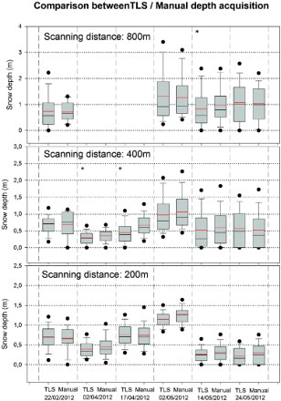
Some differences can be found in the variance of the snowpack measured with TLS and those obtained with manual measurements (Figure 5). In general, higher variances are observed in the plots 400 m and 800 m distant from the TLS in both measurements, which corresponded to areas having more complex topography relative to the flat conditions that dominated plots at 200 m distance.

Prokop (2008) found a SD accuracy within 0.1 m for distances <500 m. The accuracy increased for shorter distances, with a maximum SD deviation of ±0.08 m and a mean deviation of 0.045 m at a distance of 300 m. This explains why TLS is considered the best technology for studying snow distribution at medium distances (up to 500 meters) (i.e. Lundberg et al., 2008). Our study has revealed that mean errors lower than 0.1 m can be also obtained at longer distances, as it has been demonstrated for 800 meters. These results indicate that the protocol presented in this study minimizes error sources, and suggests the applicability of the technique for large distances (up to 800–1000m).

7. Conclusions

The SD maps generated in the study enable improved monitoring and understanding of snow dynamics in the study area. For this area of 55 ha they provide the highest resolution SD distributions maps (spatial resolution 1 m) available for the Pyrenees. In addition, the maps are not subject to interpolation uncertainties because cells with no point information were discarded.

The results of the manual and TLS measurements of SD show good performance, with only minor differences in the average values between the two measurement techniques, even for long-range TLS measurements. The increase in SD variability for medium (400 m) and large (800 m) distances are explained by differences in concavities and convexities among the selected plots and is observed in both, TLS and manual measurements. The results reinforce the applicability of this technique for studying SD distribution and its relation with topographic variables. For future studies it is recommended that SDs be measured using snow poles fixed in the terrain, which should improve the match between manual SD measurements and the SD derived from the TLS. In this way precise positioning would be achieved and manual GPS measurement uncertainties would be avoided.

Despite meteorological and stability limitations, the TLS technology was shown to generate accurate high-resolution snow distribution maps in alpine terrain, obtained by subtraction of DEMs. Long-range data acquisition from spatially distributed locations in the experimental area is a major advantage of this technology, because it enables data acquisition in remote areas that are dangerous or impossible to reach.

The application of the TLS technique in mountainous environments represents a powerful tool for understanding snow dynamics. The main objective in generating SD maps is to represent the spatial variability of snow and snow permanence over time at specific locations in the catchment.

Software

Data acquisition using the TLS was achieved using Riprofile 1.6.2^® software (Riegl, Austria). This enabled point cloud overlapping from different scan stations, and the coordinate transformations from SOCS to PRCS and to GLCS. The final point cloud coordinates were exported as ASCII files. Miramon v6.4 software was used for final rasterization of point clouds data, because it is able to manage large databases. Miramon v6.4 was also used for generating the SD maps, and ArcGis 9.3 was used to generate the final cartographies.

Acknowledgements

This work was supported by the research projects CGL2011-27536 and CGL2011-27574-CO2-02, financed by the Spanish Commission of Science and Technology and FEDER; ‘Efecto de los escenarios de cambio climático sobre la hidrologÚa superficial y la gestiæn de embalses del Pirineo Aragonés’, financed by ‘Obra Social La Caixa’; and CTTP1/12 ‘Creaciæn de un modelo de alta resoluciæn espacial para cuantificar la esquiabilidad y la afluencia turística en el Pirineo bajo distintos escenarios de cambio climático’, financed by the Comunidad de Trabajo de los Pirineos. First author is a recipient under the predoctoral grant FPU program 2010 (Spanish Ministry of Education Culture and Sports). The third author was the recipient of the postdoctoral grants JAE-DOC043 (CSIC) and JCI-2011-10263 (Spanish Ministry of Science and Innovation). We offer thanks to www.oshitoaudiovisual.com for the vectorization of the map. The authors wish to acknowledge the editor and three reviewers for their detailed and helpful comments to the original manuscript.

References

- Abellán, A., Calvet, J., Vilaplana, J. M., & Blanchard, J. (2010). Detection and spatial prediction of rockfalls by means of terrestrial laser scanner monitoring. Geomorphology, 119(3–4), 162–171. doi: 10.1016/j.geomorph.2010.03.016
- Abellán, A., Jaboyedoff, M., Oppikofer, T., & Vilaplana, J. M. (2009). Detection of millimetric deformation using a terrestrial laser scanner: experiment and application to a rockfall event. Nat. Hazards Earth Syst. Sci., 9(2), 365–372. doi: 10.5194/nhess-9-365-2009
- Abellán, A., Vilaplana, J. M., & Martínez, J. (2006). Application of a long-range terrestrial laser scanner to a detailed rockfall study at Vall de Núria (Eastern Pyrenees, Spain). Engineering Geology, 88(3–4), 136–148. doi: 10.1016/j.enggeo.2006.09.012
- Avian, M., & Bauer, A. (2006). First results on monitoring glacier dynamics with the aid of terrestrial laser scanning on Pasterze glacier (Hohe Tauem, Austria). Grazer Schriften der Geographie und Raumforschung, 41, 27–36.
- Bales, R. C., & Harrington, R. F. (1995). Recent progress in snow hydrology. Reviews of Geophysics Supplement, 33, 1011–1020. doi: 10.1029/95RG00340
- Bavera, D., & De Michele, C. (2009). Snow water equivalent estimation in the Mallero basin using snow gauge data and MODIS images and fieldwork validation. Hydrological Processes, 23(14), 1961–1972. doi: 10.1002/hyp.7328
- Birkeland, K. W., Hansen, K. J., & Brown, R. L. (1995). The spatial variability of snow resistance on potential avalanche slopes. Journal of Glaciology, 41(137), 183–190.
- Bitelli, G., Dubbini, M., & Zanutta, A. (2004). Terrestrial laser scanning and digital photogrammetry techniques to monitor landslide bodies. In International archieves of photogrammetry, remote sensing and spatial information sciences, 35 Congress, Commission V, WG V/2 (pp. 246–251).
- Colbeck, S. C., Anderson, E. A., Bissell, V. C., Crock, A. G., Male, D. H., Slaughter, C. W., & Wiesnet, D. R. (1979). Snow accumulation, distribution, melt, and runoff. Eos, Transactions American Geophysical Union, 60(21), 465–468. doi: 10.1029/EO060i021p00465
- Deems, J. S., Fassnacht, S. R., & Elder, K. J. (2006). Fractal Distribution of Snow Depth from Lidar Data. Journal of Hydrometeorology, 7(2), 285–297. doi: 10.1175/JHM487.1
- Egli, L., Jonas, T., Grünewald, T., Schirmer, M., & Burlando, P. (2012). Dynamics of snow ablation in a small Alpine catchment observed by repeated terrestrial laser scans. Hydrological Processes, 26(10), 1574–1585. doi: 10.1002/hyp.8244
- Erickson, T. A., Williams, M. W., & Winstral, A. (2005). Persistence of topographic controls on the spatial distribution of snow in rugged mountain terrain, Colorado, United States. Water Resources Research, 41(4). doi: 10.1029/2003WR002973
- Erxleben, J., Elder, K., & Davis, R. (2002). Comparison of spatial interpolation methods for estimating snow distribution in the Colorado Rocky Mountains. Hydrological Processes, 16(18), 3627–3649. doi: 10.1002/hyp.1239
- Fassnacht, S. R., & Deems, J. S. (2006). Measurement sampling and scaling for deep montane snow depth data. Hydrological Processes, 20(4), 829–838. doi: 10.1002/hyp.6119
- Groffman, P. M., Driscoll, C. T., Fahey, T. J., Hardy, J. P., Fitzhugh, R. D., & Tierney, G. L. (2001). Colder soils in a warmer world: A snow manipulation study in a northern hardwood forest ecosystem. Biogeochemistry, 56(2), 135–150. doi: 10.1023/A:1013039830323
- Gross, M. F., Hardisky, M. A., Doolittle, J. A., & Klemas, V. (1990). Relationships among depth to Frozen soil, soil wetness, and vegetation type and biomass in Tundra near Bethel, Alaska, U.S.A. Arctic and Alpine Research, 22(3), 275–282. doi: 10.2307/1551590
- Grünewald, T., Schirmer, M., Mott, R., & Lehning, M. (2010). Spatial and temporal variability of snow depth and ablation rates in a small mountain catchment. The Cryosphere, 4(2), 215–225. doi: 10.5194/tc-4-215-2010
- Heritage, G., & Hetherington, D. (2007). Towards a protocol for laser scanning in fluvial geomorphology. Earth Surface Processes and Landforms, 32(1), 66–74. doi: 10.1002/esp.1375
- Hodge, R., Brasington, J., & Richards, K. (2009). In situ characterization of grain-scale fluvial morphology using Terrestrial Laser Scanning. Earth Surface Processes and Landforms, 34(7), 954–968. doi:10.1002/esp.1780.
- Hopkinson, C., Chasmer, L., Young-Pow, C., & Treitz, P. (2004). Assessing forest metrics with a ground-based scanning lidar. Canadian Journal of Forest Research, 34(3), 573–583. doi: 10.1139/x03-225
- Jaboyedoff, M., Oppikofer, T., Abellan, A., Derron, M.-H., Loye, A., Metzger, R., & Pedrazzini, A. (2012). Use of LIDAR in landslide investigations: A review. Natural hazards, 61(1), 5–28. doi: 10.1007/s11069-010-9634-2
- Jörg, P., Fromm, R., Sailer, R., & Schaffhauser, A. (2006). Measuring snow depth with a terrestrial laser ranging system. In International snow science workshop (pp. 425–460). Presented at the International Snow Science Workshop, Telluride, Colorado.
- Jost, G., Weiler, M., Gluns, D. R., & Alila, Y. (2007). The influence of forest and topography on snow accumulation and melt at the watershed-scale. Journal of Hydrology, 347(1–2), 101–115. doi: 10.1016/j.jhydrol.2007.09.006
- Keller, F., Kienast, F., & Beniston, M. (2000). Evidence of response of vegetation to environmental change on high-elevation sites in the Swiss Alps. Regional Environmental Change, 1(2), 70–77. doi: 10.1007/PL00011535
- Körner, C. (1994). Impact of atmospheric changes on high mountain vegetation. In Mountain environments in changing climates (pp. 155–166). London: Routledge.
- Lane, S. N., Westaway, R. M., & Murray Hicks, D. (2003). Estimation of erosion and deposition volumes in a large, gravel-bed, braided river using synoptic remote sensing. Earth Surface Processes and Landforms, 28(3), 249–271. doi: 10.1002/esp.483
- Lehning, M., Völksch, I., Gustafsson, D., Nguyen, T. A., Stähli, M., & Zappa, M. (2006). ALPINE3D: a detailed model of mountain surface processes and its application to snow hydrology. Hydrological Processes, 20(10), 2111–2128. doi: 10.1002/hyp.6204
- Lichti, D. D., & Jamtsho, S. (2006). Angular resolution of terrestrial laser scanners. The Photogrammetric Record, 21(114), 141–160. doi: 10.1111/j.1477-9730.2006.00367.x
- Liston, G. E., & Sturm, M. (2002). Winter precipitation patterns in arctic alaska determined from a blowing-snow model and snow-depth observations. Journal of Hydrometeorology, 3, 646–659. doi: 10.1175/1525-7541(2002)003<0646:WPPIAA>2.0.CO;2
- López-Moreno, J. I., Fassnacht, S. R., Beguería, S., & Latron, J. B. P. (2011). Variability of snow depth at the plot scale: Implications for mean depth estimation and sampling strategies. The Cryosphere, 5(3), 617–629. doi: 10.5194/tc-5-617-2011
- López-Moreno, J. I., Latron, J., & Lehmann, A. (2010). Effects of sample and grid size on the accuracy and stability of regression-based snow interpolation methods. Hydrological Processes, 24(14), 1914–1928. .
- López-Moreno, J. I., Pomeroy, J. W., Revuelto, J., & Vicente-Serrano, S. M. (2012). Response of snow processes to climate change: Spatial variability in a small basin in the Spanish Pyrenees. Hydrological Processes. 27(18), 2637–2650. doi: 10.1002/hyp.9408
- Lundberg, A., Gustafsson, V., & Granlund, N. (2008). “Ground Truth” Snow Measurements–Review. of operational and New measurement methods fos Sweeden, Norway and Finland. In 65th eastern snow conference (pp. 215–237). Presented at the 65th Eastern Snow Conference, Fairlee (Lake Money), Vermont, USA.
- Molotch, N. P., Colee, M. T., Bales, R. C., & Dozier, J. (2005). Estimating the spatial distribution of snow water equivalent in an alpine basin using binary regression tree models: The impact of digital elevation data and independent variable selection. Hydrological Processes, 19(7), 1459–1479. doi: 10.1002/hyp.5586
- Oppikofer, T., Jaboyedoff, M., & Keusen, H.-R. (2008). Collapse at the eastern Eiger flank in the Swiss Alps. Nature Geoscience, 1(8), 531–535. doi: 10.1038/ngeo258
- Pomeroy, J., Essery, R., & Toth, B. (2004). Implications of spatial distributions of snow mass and melt rate for snow-cover depletion: Observations in a subarctic mountain catchment. Annals of Glaciology, 38(1), 195–201. doi: 10.3189/172756404781814744
- Pomeroy, J. W., & Gray, D. M. (1995). Snowcover accumulation, relocation, and management. Saskatoon, Sask. Canada: National Hydrology Research Institute. ISBN: 06601581679780660158167.
- Prokop, Alexander. (2008). Assessing the applicability of terrestrial laser scanning for spatial snow depth measurements. Cold Regions Science and Technology, 54(3), 155–163. doi: 10.1016/j.coldregions.2008.07.002
- Prokop, A. (2009). Terrestrial laser scanning for snow depth observations: An update on technical developments and applications. In International snow science workshop (Vol. 27, pp. 192–196). Presented at the International Snow Science Workshop, Davos Swizerland.
- Prokop, A., Schirmer, M., Rub, M., Lehning, M., & Stocker, M. (2008). A comparison of measurement methods: Terrestrial laser scanning, tachymetry and snow probing for the determination of the spatial snow-depth distribution on slopes. Annals of Glaciology, 49(1), 210–216. doi: 10.3189/172756408787814726
- Reshetyuk, Y. (2006). Investigation and calibration of pulsed time-of-flight terrestrial laser scanners (dissertation). KTH.
- Romanescu, G., Venedict, B., Cotiuga, V., & Asandulesei, A. (2011). Use of the 3-D scanner in mapping and monitoring the dynamic degradation of soils. Case study of the Cucuteni-Baiceni Gully on the Moldavian Plateau (Romania). Hydrology and Earth System Sciences Discussions, 8(4), 6907–6937. doi: 10.5194/hessd-8-6907-2011
- Rub, M. (2007). Terrestrial long range laser scanning for snow distribution monitoring. Zurich: Swiss Federal Institute of Technology.
- Schaffhauser, A., Adams, M., Fromm, R., Jörg, P., Luzi, G., Noferini, L., & Sailer, R. (2008). Remote sensing based retrieval of snow cover properties. Cold Regions Science and Technology, 54(3), 164–175. doi: 10.1016/j.coldregions.2008.07.007
- Schürch, P., Densmore, A. L., Rosser, N. J., Lim, M., & McArdell, B. W. (2011). Detection of surface change in complex topography using terrestrial laser scanning: Application to the Illgraben debris-flow channel. Earth Surface Processes and Landforms, 36(14), 1847–1859. doi: 10.1002/esp.2206
- Schwalbe, E., Mass, H. G., Dietrichb, R., & Ewert, H. (2008). Glacier velocity determination from multi temporal terrestrial long range scanner point clouds. In International Archives of the Photogrammetry, Remote Sensing and Spatial Information Sciences. Commission V, WG V/3 (Vol. 37, pp. 457–462).
- Siegel, S., & Castelan, N. J. (1988). Nonparametric statistics for the behavioral sciences. New York: McGraw-Hill.
- Sovilla, B. (2004). Field experiments and numerical modelling of mass entrainment and deposition processes in snow avalanches - ETH E-Collection. ETH Zürich. Diss., Technische Wissenschaften, Nr 15462.
- Ullrich, A. (2005). Atmospheric and geometric scaling correction. Internal paper of the company RIEGL laser measurement systems GmbH. Horn, Austria.
- Wagner, W., Ullrich, A., Melzer, T., Breise, C., & Kraus, K. (2004). From single-pulse to full-waveform airborne laser scanners: Potencial and practical challenges. In International Achives of Photogrametry and Remote Sciences 35. B3 (Vol. 35, pp. 201–206).
- Wehr, A., and Lohr, U. (1999). Airborne laser scanning—An introduction and overview. ISPRS Journal of Photogrammetry and Remote Sensing, 54(2–3), 68–82. doi: 10.1016/S0924-2716(99)00011-8
- Wheaton, J. M., Brasington, J., Darby, S. E., & Sear, D. A. (2010). Accounting for uncertainty in DEMs from repeat topographic surveys: Improved sediment budgets. Earth Surface Processes and Landforms, 35(2), 136–156. doi:10.1002/esp.1886.
- Williams, K. E. (2012). Accuracy assessment of LiDAR point cloud geo-referencing (Master Thesis/Dissertation). School of Civil and Construction Engineering, Oregon State Univeristy.