Flooding in ephemeral streams: incorporating transmission losses

ABSTRACT

Streamflow in semi-arid lands commonly occurs in the form of flash floods in dry-bed ephemeral streams. The goal of this research was to couple hydrological and 2D hydraulic model treatments of channel transmission losses, in order to show the impact of not taking transmission losses on flood hazard mapping into consideration. For hydraulic modeling the reach that is located between flumes 2 and 1 in the Walnut Gulch Experimental Watershed was tested. Two hydraulics models were set up, the first does not incorporate channel transmission and the second was developed to take into account several hydrographs with transmission losses as boundary conditions. The error in volume and peak runoff rate between the observed and simulated data ranges was in the order of –4.5–34.4% for runoff volume and –16.4–9.6% for peak runoff rate. The computation output interval time in the hydraulic model was 60 s and the duration of flood inundation was 6.67 h. There are important differences in depth between the two flood maps, with 0.68 maximum and 0 m minimum. The importance of using models with the dynamic treatment of transmission losses is the ability to provide an improved estimate for flood hazard mapping.

KEYWORDS:

• Transmission losses
• flood mapping
• hydrodynamic model
• hydrologic model
• ephemeral streams
• 2D numerical model

1. Introduction

The accurate characterization of watershed and channel topography has long been an integral part of geomorphological research. Nevertheless, the requirement for topographic data has changed with the shift in emphasis being from the parameterization of essentially morphological models (and concern with derived measures, such as those associated with channel cross-sectional geometry), to models with more detail and spatially explicit representation of processes (French, 2003). These concerns are especially pertinent to the latest application of high-resolution 2D and 3D models. There has been a resurgence of interest in photogrammetry as a means of producing digital elevation models (DEMs) at a wide range of scales. Of particular interest, there are developments in digital photogrammetry (e.g. Hopkinson, Hayashhi, & Peddle, 2009; Murphy, Ogilvie, Meng, & Arp, 2008; Wise, 2000) that reduce the high cost associated with traditional analytical photogrammetry as well as reducing the time taken to produce an elevation model. A more recently developed source of wide-area topographic data is airborne altimetry. In particular, airborne Light Detection and Ranging (LiDAR) systems can provide elevation and/or bathymetry measurements at a horizontal sampling interval of an order that is less than 1–5 m, with vertical accuracies in the range of ±0.10–0.15 m depending on the system configuration and flight profile (Aguilar & Mills, 2008).

Casas, Benito, Thorndycraft, and Rico (2006) analyzed the effects of the topographic data source and resolution on the hydraulic modeling of floods. Seven DEMs were generated from different altimetry sources, and the three major sources included: a global positioning system (GPS) survey and bathymetry; high-resolution LiDAR data; and vector cartography (1:5000). The hydraulic modeling was undertaken with a 1D model using all terrain models. They found that the GPS-based DEM produced more realistic water-surface elevations with variations of up to 8% in terms of flooded area but the LiDAR based model showed the greatest sensitivity to changes in Manning’s roughness coefficient.

Bates, Marks, and Horrit (2003) explored the optimum assimilation of high-resolution data into numerical models using the example of topographic data provision for flood inundation simulation. Their study consisted of: (i) an assessment of significant length scales of variation in the input data sets; (ii) determination of significant points within the data set; (iii) translation of these scales and points into a conforming model discretization that preserves solution quality for a given numerical solver; and (iv) incorporation of otherwise redundant sub-grid data in a computationally efficient manner. They recommended further studies to replicate the analysis conducted in their research for other floodplains and other high-resolution topography data sets to determine how general the conclusions regarding significant length scales are. They concluded that methods are needed to identify and connect linear topographic features in the LiDAR data, given their significant hydraulic impact. Another key unknown in flood inundation modeling is the friction surface that can also potentially be determined from LiDAR data. Frictional resistance on floodplains is dominated by drag due to vegetation. Cobby, Mason, Horrit, and Bates (2003) made a decomposition of LiDAR data using an image segmentation system that converts the LiDAR height image into separate images of surface topography and vegetation height at each point. The vegetation height map was used to estimate a friction factor at each mesh node. The spatially distributed friction model has the advantage that it is physically based, and removes the need for a model calibration exercise of friction factors. They found that using a decomposed mesh with variable friction gave a better representation of the observed flood extent than the traditional approach of using a constant floodplain friction factor. In similar research, Mason, Cobby, Horrit, and Bates (2003) investigated how vegetation data can be used to realize the currently unexploited potential of 2D flood models to specify a friction factor at each node of the finite element model mesh derived from airborne LiDAR data. They concluded that, at least for the flood event which they studied, the method of estimating variable floodplain friction using vegetation heights produced a modeled flood extent that agreed in most places with the extent observed. Nevertheless, Hladik and Alber (2012) in a study of assessment and correction of a LiDAR-derived salt marsh DEM, concluded that despite advancements in LiDAR sensor technology, state-of-the-art LiDAR applied in their investigation did not produce accurate DEMs. Errors were greatest for taller vegetation and they suggested that other vegetation characteristics should be investigated in order to understand this error.

Horrit, Bates, and Mattinson (2006) studied the effects of mesh resolution and topographic data quality on the predictions of 2D model flow using resolutions ranging from 2.5 to 50 m. Their model showed greater sensitivity to changes in mesh resolution than topographic sampling for a range of steady flow scenarios. Further, Legleiter, Kyriakidis, McDonald, and Nelson (2011) note the importance of topography data. Their study quantified the effects of uncertain topographic input data on 2D modeling of flow through a simple, gravel-bed meander bend. Results indicated that uncertain topographic input data can propagate through a 2D flow model to exert a strong influence on predictions of several key hydraulic quantities. Uncertainty associated with model predictions of water-surface elevation, depth, velocity, and boundary shear stress increased steadily, in direct proportion to the uncertainty in the topographic input data.

Marks and Bates (2000) studied the effects of topographic representation on flood inundation using topography derived from airborne LiDAR. They found that it was less subject to horizontal errors, can be rapidly collected, and repeat floodplain overflights for change detection are possible. Bilskie and Hagen (2013) recently conducted a similar experiment by integrating LiDAR data into unstructured finite element meshes using a 2D-shallow water model. They used different interpolation methods (linear, inverse distance weighted, natural neighbor, and cell averaging) to resample LiDAR and LiDAR-derived DEMs onto unstructured meshes at different resolution meshes. Their results indicate that the cell area averaging method performed best when DEM grid cells were within 0.25 times the ratio of local element size and DEM cell sizes were averaged.

A previous research study in the study site of the present investigation was carried out by Hutton, Brazier, Nicholas, and Nearing (2012) who investigated the incorporation of LiDAR into the structure of a 1D kinematic flow routing model and found it can improve the prediction of flash floods in ephemeral streams. The model was applied using two alternative model structures: using a trapezoidal representation of the cross-section and a laterally distributed cross-section derived from a 1-m-LiDAR-derived DEM. The authors concluded the integration of distributed topographic information into the LiDAR model, in the form of LiDAR-derived elevations, improved model performance, and that the most sensitive parameters were saturated infiltration and the roughness coefficient.

The goal of this research was to couple hydrological and hydraulic models in the treatment of channel transmission losses, in order to show the impact of not considering transmission losses on flood hazard mapping. In Section 2 of this paper, the study site is described and a schematic model of the coupling of both hydrological and hydraulic models is shown. Further, an independent description of each model as well as a description of the numerical method based on the Gudonov scheme and the Riemann solver are presented; In section 3, models parameterization and two flood maps (considering and not considering transmission losses) are analyzed and discussed; and finally, the conclusion of this study is in Section 4.

2. Methods

2.1. Study site

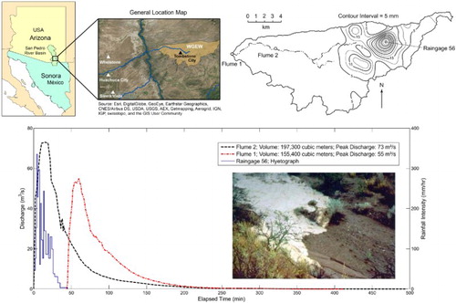
Moran et al. (2008) and associated papers provide a detailed description of the Walnut Gulch Experimental Watershed (WGEW) that is operated by the US Department of Agriculture – Agricultural Research Service (ARS). The WGEW encompasses ∼149 km² in southeastern Arizona, USA (31°43′N, 110°41′W) that surrounds the historical western town of Tombstone. The watershed is contained within the upper San Pedro River Basin that encompasses 7600 km² in Sonora, México, and Arizona. The watershed is representative of approximately 60 million ha of brush and grass covered rangeland found throughout the semi-arid southwest and is a transition zone between the Chihuahua and Sonora Deserts. Watershed elevations range from 1250 to 1585 m MSL. Walnut Gulch, being dry about 99% of the time, is an ephemeral tributary of San Pedro River (Goodrich, Williams, Unkrich, Hogan, & Scott, 2004). For hydraulic modeling the reach which is between flumes 2 and 1 was tested. The rainfall event that occurred on 27 August 1982 was modeled (Figure 1). This rainfall event occurred almost exclusively in the upper watershed. Therefore, the study reach between flume 2 and the WGEW outlet at flume 1 would have little or no lateral runoff inflow into the channel reach.

Figure 1. Location map of WGEW, transmission losses in flumes 1 and 3 hydrographs, and the 27 August 1982 hyetograph.

2.2. Coupling of hydrologic and hydraulic models

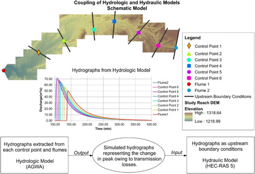
Once simulated and calibrated, the hydrologic model for the 27 August 1982 event, hydrographs with transmission losses at each control point and flumes 1 and 2 were obtained; these hydrographs worked as upstream boundary conditions at each segment modeled within the hydraulic model in order to perform the flood mapping that considers transmission losses; the hydraulic model is not capable of getting rid of water down the reach by itself. Further flood mapping (without transmission losses) was performed over the entire reach with only one hydrograph (flume 2) as the upstream boundary condition. Both flood maps are analyzed and discussed in Section 3. A schematic model of the coupling of hydrologic and hydraulic models is depicted in Figure 2.

Figure 2. Schematic model: coupling of hydrologic and hydraulic models.

2.3. Hydrologic model

The Automated Geospatial Watershed Assessment (AGWA – www.tucson.ars.ag.gov/agwa/) is a geographical information system (GIS) tool used to parameterize, execute, and spatially display simulation results from the Soil and Water Tool (SWAT2000) and the Kinematic Runoff and Erosion (KINEROS2) hydrologic models. These models operate at different temporal and spatial scales and may be applied in a range of environmental conditions to evaluate the impacts of land-cover change on hydrologic and erosion responses (Miller et al., 2007). KINEROS2 (Goodrich et al., 2012 – www.tucson.ars.ag.gov/kineros/) is a process-based model that simulates the production of excess rainfall and its conversion to surface runoff under conditions of infiltration-excess (Hortonian overland flow); it provides information on the response of a modeled watershed to land-cover and rainfall changes. However, this model is highly dependent on spatially distributed data, the subdivision of watersheds into response units, and the assignment of appropriate parameters that are both time-consuming and computationally complex. AGWA was developed under the following guidelines: (i) that its parameterization routines be simple, direct, transparent, and repeatable; (ii) that it be compatible with commonly available GIS data layers; and (iii) that it be useful for assessment and scenario development (alternative futures, land-cover, and land-use changes) at multiple scales. AGWA is an extension for Esri ArcGIS (Miller et al., 2007).

KINEROS2 was produced at the USDA-ARS. It is a distributed model that is applicable to scales from plot to watershed and it has been successfully calibrated and validated on experimental watersheds with high-resolution inputs and observations up to 150 km² in size. KINEROS2 is an even-based model that estimates runoff, erosion, and sediment transport in overland flow (hillslope), channel, detention pond, urban, injection, and non-pressurized culvert model elements. Precipitation inputs are typically in the form of rain gauge observations in either time and accumulated rainfall pairs or time intensity pairs, or radar-rainfall intensity estimates provided at time scales of tens of minutes or less. Internal computational time steps are automatically adjusted to satisfy the Courant condition (Roberts, 2003), and output time steps are user-defined (Goodrich et al., 2012).

In KINEROS2, the watershed being modeled is conceptualized as a collection of spatially distributed model elements. The model elements effectively abstract the watershed into a series of shapes that can be oriented so that one-dimensional flow can be assumed. Within each modeling element the kinematic wave equations, coupled with the Parlange three-parameter model for this process (Parlange, Lisle, Braddock, & Smith, 1982) are solved using a four-point implicit finite difference method using either the Manning or Chézy hydraulic resistance laws. Further, user-defined subdivision can be made to isolate hydrologically distinct portions of the watershed if desired (e.g. large impervious areas, abrupt changes in slope, soil type, or hydraulic roughness). Watershed characterization is important to estimate both the geometric characteristics of watershed modeling elements (e.g. slope, flow length, and area) and the factors affecting infiltration and routing (e.g. soil hydraulic properties, hydraulic roughness, land use, and land cover). Ideally, a high-resolution topographic survey data derived from LiDAR would be available for topographic and geometric characterization. Infiltration characteristics would ideally be derived from a distributed set of tension infiltometer or rainfall simulator measurements, coupled with soil textural and bulk density analyses that are sufficient to characterize the variability of the fields that is commensurate with the model’s geometric complexity. In all cases, the input, state, output, and basin characterization data should be carefully screened for outliers, errors, and temporal trends and for temporal record discontinuities (Goodrich et al., 2012).

KINEROS2 was developed explicitly with ephemeral channel routing of runoff in mind. As it features overland flow routing in the model (hillslope), channel routing of runoff is interactive with infiltration at each finite difference node. This is especially important when the front of a flood wave is traversing a dry channel. To simulate ephemeral channel transmission losses (TL) between flumes 2 and 1, six channel element end points (transmission loss control points) were forced in the model discretization along this channel reach. This enabled the extraction of channel transmission losses in each of the reaches between control points from the KINEROS2 event simulation. The model was calibrated to match the observed runoff from flume 2 with the simulated hydrograph at this location. Two issues were carefully matched, the shape of the hydrograph and discharge peak.

2.4. Hydraulic model

The motion of a fluid is governed by the physical principles of conservation of mass (continuity equation) and momentum (Navier–Stokes equation). In a cartesian frame of reference (x,y,z), given an arbitrary control volume (V) of a fluid element and Ω as its boundary, it is assumed that a free surface is present and the fluid is incompressible with constant density ρ and the equations of continuity and momentum are:(1) $\begin{array}{rl}& \underset{\mathrm{\Omega }}{\int }\mathbf{n}\ast \mathbf{u}d\mathrm{\Omega }=0,\underset{V}{\int }\frac{\mathrm{\partial }}{\mathrm{\partial }t}\left(\mathbf{u}\right)dV=\\ & \underset{V}{\int }gdV-\frac{1}{\rho }\underset{\mathrm{\Omega }}{\int }p\mathbf{n}d\mathrm{\Omega }+\frac{\mu }{\rho }\underset{\mathrm{\Omega }}{\int }\frac{\mathrm{\partial }\mathbf{u}}{\mathrm{\partial }\mathbf{n}}d\mathrm{\Omega },\end{array}$(1) where n is the unit vector outward from the boundary Ω; u=[u,v,w] is the vector of the velocity components in the x, y, and z directions, respectively; g=[g_x,g_y,g_z] represents the vector of the components of external forces per unit mass; p is the pressure; and μ is the dynamic viscosity.

This equation is applicable to describing the motion of water with a free surface under gravity. The body force vector g is assumed [0, 0, -g], where g is the acceleration due to gravity which is considered as constant and equal to 9.81 m/s². X–y axes determine a horizontal plane, while z defines the vertical direction, to which the free surface elevation is associated. The domain on which the equations have to be solved is bounded by the bottom b and the free surface η, which are defined, respectively, by the functions:$\text{Bottom}:z=b(x,y),$ $\text{free}\text{surface}:z=\eta (x,y,t)=b(x,y)+h(x,y,t),$where h (x,y,t) is the depth of water.

The free surface is a boundary and, as such, the boundary conditions have to be satisfied. However, the free surface position is unknown, hence the domain on which the equations have to be solved is not known a priori (more information on parameters in shallow water equations (SWE) can be found in Korichi & Hazzab, 2010). Approximation assumptions allow simplification of this problem. In the particular case of shallow water theory, small water depths with respect to the wave length or free surface curvature are typically assumed. This leads to a non-linear initial value problem (Toro & Navarro-Garcia, 2007)

2.5. Numerical method based on the Gudonov scheme and the Riemann solver

Gudonov-type finite-volume schemes assume piecewise solutions of the flow variables that are discontinuous at cell faces. The discontinuities are typically used by the Roe (1981) approximate Riemann solver to compute mass and momentum fluxes in order to update the solution over time. Such models are popular because they are accurate in subcritical and supercritical flow, capture hydraulic jumps and bores without special fixes, conserve mass, and their predictions are oscillation free (Begnudelli, Sanders, & Bradford, 2008). Several researchers have adopted triangular, unstructured grid formulations of Gudunov-type shallow water models (e.g. Duan & Yu, 2014; Garcia-Navarro, Hubbard, & Priestley, 1995; Yoon & Kang, 2004).

For a number of hyperbolic systems, including the SWE, it is possible to find the exact solution of the Riemann problem (Toro & Navarro-Garcia, 2007). The Riemann problem is an initial value problem, in which the governing equations are coupled with piecewise constant data imposed at the left side and at the right side of x=0, where the discontinuity is placed. The SWE are discretized by the Godunov-type finite-volume method (Toro, 2009) over a regular Cartesian mesh.

Two hydraulic models were set up on the channel reach between flumes 2 and 1. The first hydraulic model does not incorporate channel transmission losses, and the upstream boundary condition was the hydrograph simulated at flume 2 by the KINEROS2 model. The downstream boundary condition was the stage-flow rating curve from Walnut Gulch supercritical flume 1 and associated stage observations for the 27 August 1982 event (detailed information on Walnut Gulch supercritical flumes can be found in Smith, Chery, Renard, & Gwinn, 1982). The parameter filters and face conveyance ratio used were the same as for the simulation without transmission losses. The second hydraulic model was developed to take into account channel transmission losses. The flume 2 to flume 1 channel reach was divided into seven 2D areas and the limits of these areas were the control points used as channel model element breaks in the hydrologic model. For this hydraulic simulation, each area represents one small mesh with independent boundary conditions (hydrographs for each control point) and parameter filters and the face conveyance ratios used were the same for the simulation without transmission losses.

3. Results and discussion

Sensitivity analysis showed that the most sensitive parameters in this semi-arid watershed for the overland flow elements in descending order of importance were soil saturated hydraulic conductivity (K_s) values, Manning’s roughness, and vegetation cover and interception values. Hutton et al. (2012) also found the same parameters to be the most sensitive. The errors in volume and peak runoff rate between the observed and simulated data for flume 2 were −4.50% and 1.78%, respectively. For both simulated runoff volume and peak flow rate the largest errors were associated with a sub-watershed. Looper, Vieux, and Moreno (2012) found larger errors in their study but viewed them as acceptable for further analysis. Besides the infiltration and routing parameters, the channel geometry (width and banks slope) was estimated using LiDAR DEM data.

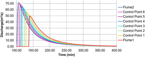
For each control point along the channel between flumes 2 and 1 the simulated hydrograph was extracted, representing the change in peak owing to transmission losses from the start to the end of the channel, and these hydrographs are shown in Figure 3. Each of the hydrographs produced by the KINEROS2 hydrologic model, which treats channel transmission losses, was used as input to the hydraulic model at the respective control points. This simulation was compared to the routing with no transmission losses using the hydraulic model between flumes 2 and 1.

Figure 3. Simulated hydrographs from control points between flumes 2 and 1 for the 27 August 1982 event.

Several programs were used to set up, execute, and map the hydraulic model simulation results including: (i) Geometry preprocessor; (ii) Unsteady flow simulation (w/o sediment transport); (iii) Post processor; and (iv) Floodplain mapping. Both simulations took between 4 and 5 h to complete. The results in flood depth for the studied channel are shown in the Main Map. The first flood map illustrates the mapping when transmission losses are accounted for. In the second one they are not modeled.

Differences can be seen in the southern secondary channel in the section between UTM coordinates Eastings 583,500 and 584,000 m which is fully connected with a non-zero flow depth in the second flood map and is not in first one owing to reduced runoff discharge from channel transmission losses. Detailed zones with important differences are depicted on the left-hand side of the general description section of the map.

There are important differences between the two flood mappings due to the way the hydraulic model treats the input (upper) hydrograph in each sub-reach. It was found that the hydrograph in the output of each is similar to the input hydrograph in the next area in terms of shape, but not necessarily in terms of volume. Notwithstanding, the flood mapping has important differences.

The differences were computed by subtracting the simulations with TL from the simulation without TL. There are differences in depth up to approximately 0.68 as maximum and 0 m as minimum. In the histograms shown in Figure 4 for the simulation with transmission losses (TL – on the left) and without TL (right) the number of cell elements with depths less than 0.9 m are similar, but for elements with greater depths the histograms have different behavior. As expected, there are more cells in the small depth ranges. Both flood mappings (with and w/o transmission losses) have a similar coefficient of variation (0.70 and 0.73, respectively). This is due to the reduction in mean and standard deviation when TL are considered. This does not imply that the differences in flood mappings with and without TL are minor.

Figure 4. Flood mapping histograms.

4. Conclusions

Many hydrologic models do not interactively treat infiltration and routing simultaneously but rather abstract infiltration from a hyetograph and so route the effective rainfall down an impervious representation of the watershed. This approach is not able to represent the dynamics of transmission losses in intermittent and ephemeral channels for each step in the simulation. In these types of stream systems the dynamic treatment of transmission losses will provide a more realistic simulation of runoff. Using these hydrographs as input into a 2D hydraulic model improves flood mapping for forecasting areas of flood hazard. The methodology described in this paper enabled the application of a 2D hydraulic model that does not currently treat channel transmission losses related to the gauged ephemeral channels in the WGEW.

This research modeled events with transmission losses. It is important for future research to model more and bigger events. In the event under study, the percentage of lost volume was considered important, but smaller or larger overall transmission losses can be considered important in order to evaluate the impact of transmission losses on flood mapping.

Software

HEC-RAS 5.0 (developed by the US Army Engineer Institute for Water Resources) was used to create both water depth DEMs. AGWA is an Esri ArcGIS extension (Miller et al., 2007) and was used to generate the hydrologic maps, as well as the general map.

Disclosure statement

No potential conflict of interest was reported by the authors.

References

- Aguilar, F. J., & Mills, J. (2008). Accuracy assessment of LiDAR-derived digital elevation models. The Photogrammetric Record, 23(122), 148–169. doi:10.1111/j.1477-9730.2008.00476.x
- Bates, P. D., Marks, K. J., & Horrit, M. S. (2003). Optimal use of high-resolution topographic data in flood inundation models. Hydrological Processes, 17, 537–557. doi: 10.1002/hyp.1113
- Begnudelli, L., Sanders, B. F., & Bradford, S. F. (2008). Adaptive Gudunov-based model for flood simulation. Journal of Hydraulic Engineering, 134(6), 714–725. doi:10.1061/(ASCE)0733-9429(2008)134:6(714)
- Bilskie, M. V., & Hagen, S. C. (2013). Topographic accuracy assessment of bare earth LiDAR-derived unstructured meshes. Advances in Water Resources, 52, 165–177. doi: 10.1016/j.advwatres.2012.09.003
- Casas, A., Benito, G., Thorndycraft, V., & Rico, M. (2006). The topographic data source of digital terrain models as a key element in the accuracy of hydraulic flood modeling. Earth Surface Processes and Landforms, 31, 444–456. doi: 10.1002/esp.1278
- Cobby, D. M., Mason, D. C., Horrit, M. S., & Bates, P. D. (2003). Two-dimensional hydraulic flood modeling using a finite element mesh decomposed according to vegetation and topographic features derived from airborne scanning laser altimetry. Hydrological Processes, 17, 1979–2000. doi: 10.1002/hyp.1201
- Duan, J., & Yu, C. (2014). Two-Dimensional hydrodynamic model for surface-flow routing. Journal of Hydraulic Engineering, 04014045, 1–13.
- French, J.R. (2003). Airborne LiDAR in support of geomorphological and hydraulic modelling. Earth Surface Processes and Landforms, 28, 321–335. doi:10.1002/esp.484
- Garcia-Navarro, P., Hubbard, M., & Priestley, A. (1995). Genuinely multidimensional upwinding for the 2D shallow water equations. Journal of Computational Physics, 121, 79–93. doi: 10.1006/jcph.1995.1180
- Goodrich, D. C., Burns, I. S., Unkrich, C. L., Semmens, D. J., Guertin, D. P., Hernandez, M., … Levick, L. R. (2012). KINEROS2/AGWA: Model Use, calibration, and validation. Transactions of the American Society of Agricultural and Biological Engineers, 55(4), 1561–1574.
- Goodrich, D. C., Williams, D. G., Unkrich, C. L., Hogan, J. F., & Scott, R. L. (2004). Comparison of methods to estimate ephemeral channel recharge, Walnut Gulch, San Pedro river basin, Arizona. Water Science and Application, 9, 77–99. doi: 10.1029/009WSA06
- Hladik, C., & Alber, M. (2012). Accuracy assessment and correction of a LiDAR-derived salt marsh digital elevation model. Remote Sensing of Environment, 121, 224–235. doi: 10.1016/j.rse.2012.01.018
- Hopkinson, C., Hayashhi, M., & Peddle, D. (2009). Comparing alpine watershed attributes from LiDAR photogrammetric, and contour-based digital elevation models. Hydrological Processes, 23, 451–463. doi: 10.1002/hyp.7155
- Horrit, M. S., Bates, P. D., & Mattinson, M. J. (2006). Effects of mesh resolution and topographic representation in 2D finite volume models of shallow water fluvial flow. Journal of Hydrology, 329, 306–314. doi: 10.1016/j.jhydrol.2006.02.016
- Hutton, C., Brazier, R., Nicholas, A., & Nearing, M. (2012). On the effects of improved cross-section representation in one-dimensional flow routing models applied to ephemeral rivers. Water Resources Research, 48, W04509. doi:10.1029/2011WR011298
- Korichi, K., & Hazzab, A. (2010). Application of shock capturing method for free surface flow simulation. Jordan Journal of Civil Engineering, 4, 310–320.
- Legleiter, C. J., Kyriakidis, P. C., McDonald, R. R., & Nelson, J. M. (2011). Effects of uncertain topographic input data on two-dimensional flow modeling in a gravel-bed river. Water Resources Research, 47, W03518. doi:10.1029/2010WR009618
- Looper, J. P., Vieux, B. E., & Moreno, M. A. (2012). Assessing the impacts of precipitation bias on distributed hydrologic model calibration and prediction accuracy. Journal of Hydrology, 418–419, 110–122. doi: 10.1016/j.jhydrol.2009.09.048
- Marks, K., & Bates, P. (2000). Integration of high-resolution topographic data with floodplain flow models. Hydrological Processes, 14, 2109–2122. doi: 10.1002/1099-1085(20000815/30)14:11/12<2109::AID-HYP58>3.0.CO;2-1
- Mason, D. C., Cobby, D. M., Horrit, M. S., & Bates, P. D. (2003). Floodplain friction parameterization in two-dimensional river flood models using vegetation heights derived from airborne scanning laser altimetry. Hydrological Processes, 17, 1711–1732. doi: 10.1002/hyp.1270
- Miller, S. N., Semmens, D. J., Goodrich, D. C., Hernandez, M., Miller, R. C., Kepner, W. C., & Guertin, D. P. (2007). The automated geospatial watershed assessment tool. Environmental Modelling & Software, 22, 365–377. doi: 10.1016/j.envsoft.2005.12.004
- Moran, M. S., Holifield, C., Goodrich, D. C., Qi, J., Shannon, D. T., & Olsson, A. (2008). Long-term remote sensing database, Walnut Gulch experimental watershed, Arizona, United States. Water Resources Research, 44, W05S10. doi:10.1029/2006WR005689
- Murphy, P., Ogilvie, J., Meng, F.-R., & Arp, P. (2008). Stream network modelling using LiDAR and photogrammetric digital elevation models: A comparison and field verification. Hydrological Processes, 22, 1747–1754. doi: 10.1002/hyp.6770
- Parlange, J.-Y., Lisle, I., Braddock, R. D., & Smith, R. E. (1982). The three-parameter infiltration equation. Soil Science, 133(6), 337–341. doi: 10.1097/00010694-198206000-00001
- Roberts, A. J. (2003). A holistic finite difference approach models linear dynamics consistently. Mathematics of Computation, 72(241), 247–263. doi: 10.1090/S0025-5718-02-01448-5
- Roe, P. L. (1981). Approximate Riemann solvers, parameter vectors, and difference schemes. Journal of Computational Physics, 43, 357–372. doi: 10.1016/0021-9991(81)90128-5
- Smith, R. E., Chery, D. L., Renard, K. G., & Gwinn, W. R. (1982). Supercritical flow flumes for measuring sediment-laden flow. Technical Bulletin Number 1655. Agricultural Research Service. U.S. Department of Agriculture.
- Toro, E. (2009). Riemann solvers and numerical methods for fluid dynamics: A practical introduction (3rd ed.). Berlin: Springer.
- Toro, E., & Navarro-Garcia, P. (2007). Godunov-type methods for free-surface shallow flows: A review. Journal of Hydraulic Research, 45(6), 736–751. doi:10.1080/00221686.2007.9521812
- Wise, S. (2000). Assessing the quality for hydrological applications of digital elevation models derived from contours. Hydrological Processes, 14, 1909–1929. doi: 10.1002/1099-1085(20000815/30)14:11/12<1909::AID-HYP45>3.0.CO;2-6
- Yoon, T. H., & Kang, S.-K. (2004). Finite volume model for two-dimensional shallow water flows on unstructured grids. Journal of Hydraulic Engineering, 130(7), 678–688. doi:10.1061/(ASCE)0733-9429(2004)130:7(678)