Shrinkage prediction and correction in material extrusion of cellulose-chitin biopolymers using neural network regression

ABSTRACT

Loss of geometric accuracy due to shrinkage is a challenge in material extrusion of biological composites using water-based inks, such as the cellulose-chitin biopolymers used here. The shape of 3D printed objects often departs from the intended design geometry due to evaporative loss of water during curing. Moreover, such materials' viscoelastic characteristics result in complex volumetric changes that are difficult to predict and compensate for. We developed a prediction-correction scheme by 3D printing and scanning cylindrical and conic surfaces, computing the geometric deviations between designed and cured artefacts, and training a neural network such that given the machine path for a 3D print, the model can predict shrinkage deformations and apply adjustments on the generating machine paths to proactively compensate it. In this article, we present the shrinkage characteristics of the material used and the results of applying the predictor-correction scheme. The approach substantially improves geometric accuracy, enabling nearly seamless assembly of separately 3D printed parts. Addressing such a fundamental problem of quality control as geometric accuracy may enable the broader adoption of biopolymers and potentially displace the generalised use of synthetic plastics.

KEYWORDS:

• Material extrusion
• cellulose-chitin biopolymers
• shrinkage compensation
• neural network regression

Introduction

While Additive Manufacturing (AM) offers several advantages over earlier forms of fabrication, several challenges persist regarding the quality of its end products (Kruth, Leu, and Nakagawa 1998; Tofail et al. 2018). Quality is typically assessed based on the manufactured objects’ geometric, mechanical, and physical characteristics (Mani et al. 2015). Geometric criteria include dimensional accuracy, surface roughness and feature resolution (Rebaioli and Fassi 2017). Dimensional accuracy, in the sense of the geometric deviation between designed and manufactured artefacts, is a critical property (Lee et al. 2014). Object synthesis at a relatively smaller scale than the final artefact requires material fusion and state transition, resulting in complex phenomena such as shrinkage and warpage (Bikas, Stavropoulos, and Chryssolouris 2016). Loss of geometric accuracy is influenced by several factors including material properties, system parameters, and environmental factors, such as the polymer’s crystallinity in material extrusion (Spoerk et al. 2017), binder quantity (Kafara et al. 2018) and particle size in binder jetting (Mostafaei et al. 2019), temperature variations in laser sintering (Dastjerdi, Movahhedy, and Akbari 2017; Soe, Eyers, and Setchi 2013; Zago et al. 2021). Mitigation of those quality control problems is often approached via industrial process control methodology (Turner and Gold 2015). This article presents a study on improving the dimensional accuracy of material extrusion using natural biological materials; namely cellulose-chitin biopolymers. The use of cellulose-chitin biopolymers aims at sustainable AM by substituting synthetic plastics with naturally abundant, widely available, low-cost, renewable, and biodegradable materials (Sanandiya et al. 2018). Despite their appealing characteristics, due to the high content of water as well as the innate variability of its organic components, 3D printed artefacts undergo significant geometric changes during curing. Shrinkage of chitinous biopolymers, and more broadly hydrogel inks, is the result of dehydration during curing (Rajabi et al. 2021). Limitations in dimensional accuracy must be therefore overcome to enable the adoption of biopolymer AM for industrial applications.

Relevant work

Improvement of dimensional accuracy may be achieved in one of the following ways: (a) Pre-processing or off-line, by taking proactive measures before 3D printing, such as analysing the design geometry, predicting errors, and modifying machine paths (Moroni, Syam, and Petrò 2014). (b) In-process or online, by performing corrections during 3D printing, such as monitoring for errors and adjusting process control settings dynamically (Liu and Li 2004; Spears and Gold 2016). (c) Post-processing, namely performing additional finishing steps after 3D printing or employing hybrid manufacturing techniques such as (Strong et al. 2018; Mayur et al. 2018).

Compensation against geometric errors has been approached in the past using: (a) Analytical models associated with the material, geometry and/or the mechanical system used. Indicative examples include developing a melting model for polymers used in fused filament fabrication (Osswald, Puentes, and Kattinger 2018), modelling the motion characteristics of the 3D printer in material extrusion (Tong, Joshi, and Lehtihet 2008; Moroni, Syam, and Petrò 2014), and creating an optics model for dimensional accuracy improvement in vat photopolymerization (Guven, Karpat, and Cakmakci 2022). (b) Physics simulation methods such as simulating the transient thermal and chemical effects of resin-curing in vat photopolymerization (Tang et al. 2004) and employing finite-elements modelling for dimensional improvement in powder bed fusion (Kakanuru and Pochiraju 2022). (c) Empirical studies using experimental modelling techniques such as using a process parameter control model to improve surface quality for binder jetting (Chen and Zhao 2016) and developing error models using coordinate measurement machinery for performing powder bed fusion error compensation (Brøtan 2014).

Experimental methods for improving dimensional accuracy, such as the one presented here, are often based on statistical techniques such as the design of experiment (Chen and Zhao 2016), response surface modelling (Lynn-Charney and Rosen 2000), Markov chain and Monte Carlo strategies (Huang et al. 2015), multi-objective optimisation (Pavan and Srinivasa 2014), Bayesian inference modelling (Nath et al. 2020; Yang et al. 2022), support vector machines (Delli and Chang 2018) as well as artificial neural networks (Noriega, Blanco, and Alvarez 2013; Chowdhury and Anand 2016; Hong et al. 2021). Machine learning (ML), also used here, became popular with the emergence of efficient parallel computing hardware in the past few decades. Indicative quality control applications for AM include process settings control (Muñiz Castro et al. 2021), online error detection using computer vision and convolutional neural networks (Kim et al. 2020; Farhan Khan et al. 2021; Corradini and Silvestri 2022), closed-loop detection and correction by adjustment of process settings in material extrusion (Goh, Hamzah, and Wai 2021). Neural networks are capable of accounting for complex interactions between process parameters (Noriega, Blanco, and Alvarez 2013) and addressing highly non-linear problems (Hong et al. 2021) such as material shrinkage.

Objectives and approach

The objective of this work is to overcome the challenge of shrinkage in cellulose-chitin biopolymer extrusion which prevents its adoption for industrial applications. We developed ML models, to predict and compensate for dimensional inaccuracies by adjusting machine paths before 3D printing. The approach was motivated by the non-linear attributes of the material shrinkage characteristics, presented later in this document, and the prohibitive complexity of developing a transient multi-physics simulation model. Instead, the ease of directly 3D printing artefacts, and the availability of affordable 3D scanning equipment, graphics processing units, and ML frameworks, offered a plausible alternative. ML regression is employed to ingest empirical data over time and compose an ever-improving prediction-correction mechanism. Moreover, the investigation aimed to assess whether an ML model can perform localised corrections using a limited amount of information in the vicinity of a machine path location, instead of seeing the entire geometry. It was also desirable to assess whether an ML model can account for special conditions of shrinkage, such that at the interface of the material with the base plate. Finally, the layer breadth and depth of several neural networks were investigated to understand the complexity of the model required. The article first presents an overview of the material and 3D printing process characteristics, followed by a detailed exposition of shrinkage measurement and analysis, a presentation of the modelling technique, and an experimental evaluation of the achieved improvements.

Materials and methods

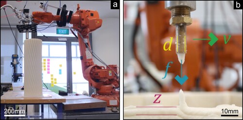
Additive manufacturing with our cellulose-chitin biopolymers is based on material extrusion similar to fused filament fabrication and direct ink writing. The system is comprised of an articulated 6-axis robotic positioner, with a notional 1.65 m horizontal and 3.7 m vertical reach, equip with a viscous materials extrusion pump and a volumetric dispenser for adhesives and sealants, see Figure 1(a). The material is a colloid dispersion of chitin and cellulose with ratio 1:8 by weight. Chitin is dissolved in water at a 3% concentration, using acetic acid in a 1% solution. The dynamic viscosity of the ink is circa 1500 Pa.s. The mechanical and physical properties of the material, after curing, are in the range of synthetic foams and natural timbers with 0.26 GPa Young's modulus and 0.37 g/cm3 density.

Figure 1. (a) Large-scale AM system featuring an articulated robotic arm and a viscous materials dispenser printing a large-scale prototype. (b) Process control parameters include the motion velocity v, flow of material extrusion f, spacing between layers z, and nozzle diameter d.

Process parameters

3D printing cellulose-chitin biopolymers require no thermal input as the material is prepared, dispensed, and cured at room temperature. Hardening takes place as air convection causes water to evaporate. Key benefits of this low-energy deposition method are in increased printing speeds, at even large internal nozzle diameters, because the material does not need to melt before being extruded, thus neither stalling linear motion nor requiring elevated pumping pressures at the nozzle. Typical process parameters include linear motion speeds of 50 mm/sec, a flow rate of 115cc/min, and with 7 mm nozzle diameter, see Figure 1(b). Coordinating those parameters was approached using response surface modelling and multi-response optimisation methodology in the past and presented by (Vijay et al. 2019). To ensure repeatable results, the robot’s axis counters were calibrated, and the work envelope was restricted to the dimensions of the laser-cut acrylic plates measuring 290 mm by 240 mm used as removable 3D printing bases positioned at the same location.

Specimen geometry

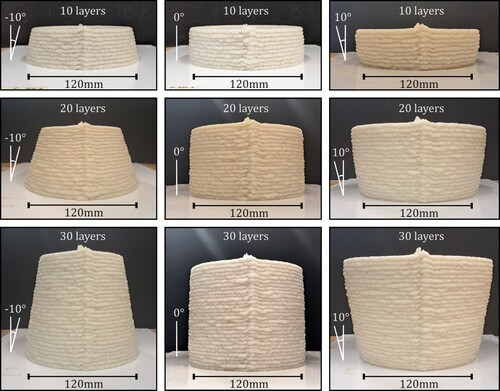
For measuring, analysing, and mitigating geometric deviation between design and 3D printed objects, several specimens were produced. Cylindrical and conic surfaces were printed, see Figure 2, with diameters of 80 (n = 5), 100 (n = 45), 120 (n = 44), 140 (n = 7), and 160 (n = 5) millimetres; taper angles of −10 (n = 14), −5 (n = 14), 0 (n = 54), 5 (n = 13) and 10 (n = 11) degrees from the vertical; and 10 (n = 17), 15 (n = 12), 20 (n = 47), 25 (n = 10) and 30 (n = 20) number of layers. Machine paths were derived by contouring those surfaces, using an initial vertical offset of 5 mm from the base plate, and 3.5 mm layer-to-layer height. Contours were segmented by chord length of 5 mm to generate polygonal machine paths for 3D printing, where the sequence of points represents the centre of the dispenser’s nozzle. The use of this family of surfaces was driven by their simplicity in measurement, registration, and establishing correspondences between desired and acquired geometries.

Figure 2. Examples of 3D printed surfaces with 120 mm diameter at the base and 10, 20, and 30 layers with −10, 0, and +10 degrees of taper angle from the vertical direction.

Measurement and registration

Measurement was performed using structured light 3D scanning equipment, with a point accuracy of 0.1 mm and resolution of 0.5 mm. Each specimen was scanned immediately after being printed and once again after it was cured. The process of scanning each object using structured light required 5 min for acquisition and less than an hour for post-processing sensor data to produce 3D mesh models. While layers are visually discernible in the meshes generated, see Figure 3(a), the scanner’s resolution, in both the geometry and texture domains, was insufficient for computationally detecting their boundaries consistently, see Figure 3(b). Surface roughness was measured using a laser profile scanner with 0.1 mm resolution, see Figure S1. The meshes extracted thus offer only an approximation of the overall shape rather than a precise location of the material run profiles per layer. Surface roughness offers an indication of the variation expected over the general shape.

Figure 3. (a) Structured-light 3D scanning equipment acquiring cylindrical specimens. (b) Details of resulting mesh geometry generated. (c) Registration procedure steps.

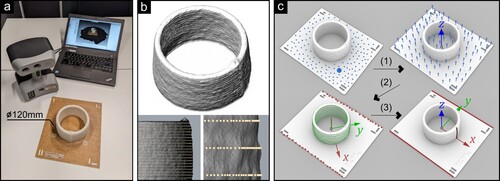
Measuring errors and training the predictive model requires establishing pairwise correspondences between design geometries and printed artefacts, namely between machine path points, which lie at the centre of the extruder's nozzle, and contour points extracted from 3D scanned objects’ surfaces. The first step of this process requires performing registration, where the acquired meshes are brought in alignment with their associated generating machine paths. Registration was performed, see Figure 3(c), using the following procedure: (1) Meshes were first aligned vertically from the sensor's arbitrary ℝ3 frame to the world's Z-direction. From the base plate, a seeding mesh vertex was manually selected, and all other connected vertices up to 1-degree vertex normal angle deviation. Principal Components Analysis (PCA) was performed using the selected vertices to recover the plate’s normal direction and vertical offset. (2) The horizontal translation, to bring the cylinders’ and cones’ centres at (x, y) = (0, 0), was recovered using the mean (x, y) among the centres of regression circles fitted to horizontal contours extracted via mesh-plane intersection, at as many vertical offsets as the number of layers. (3) Finally, the meshes were rotated about the Z-axis such that the extrusions’ start points were aligned with the positive X-axis. This orientation was recovered from the base plate’s longest boundary vertices, using PCA regression. In both steps 1 and 3 handedness for the Z and X axes was manually selected. With all meshes registered, 360 points from the top surfaces of both wet and dry meshes were extracted for computing the mean height and vertical shrinkage. This shrinkage ratio was used for vertically scaling the machine path contours to bring them into the context of the cured geometries. For cylindrical, conic, and generally convex surfaces, correspondence mapping can now be performed by projecting from the scaled machine path positions, along the in-plane surface normal direction, onto the surface of the mesh geometry.

Prediction and correction

The models developed for predicting the geometric deformations of 3D printed objects are based on deep neural networks. The inputs to the models are 7-dimensional vectors representing machine path locations and their outputs are 2-dimensional displacement vectors onto the 3D printed objects’ surfaces. Inputs encode the following properties per machine path location: (1) x-coordinate, in mm; (2) y-coordinate, in mm; (3) vertical layer index; (4) number of layers above; (5) local taper angle against the vertical direction, in degrees; (6) horizontal curvature; and (7) vertical curvature. Input vectors contain both absolute and relative geometric information. The intent for using absolute XY-coordinates is aimed at training the model to account for the positional accuracy of the robot, which is not constant across its work envelope previously studied (Hoo, Dritsas, and Fernandez 2022). The use of the layer index and number of layers above aims at hinting at the local vertical loading conditions. The taper angle and curvatures aim at capturing the local geometric features. Input vectors were scaled by normalisation factors, such that their values were approximately in the [−1, 1] domain, to avoid numerical problems with gradient descent training. Output vectors directly encode the x, and y deltas between the machine path and the corresponding surface points, also normalised in [−1, 1].

The regression models trained are based on neural networks with a fixed number of fully connected layers (FCL), using ReLU activations. Models were developed using the Pytorch framework and trained using the Adam optimiser with an initial learning rate of 0.01 and betas (0.9, 0.999), cosine annealing learning rate scheduler, and the mean square error (MSE) loss function. The models were trained using an RTX3080 graphics processing unit, over 100 epochs with each model requiring approximately 4 h of training. The size of the dataset, from 102 cylinders and cones, was approximately 600 K vector pairs, with 10% used for validation. Various models with different configurations were trained and evaluated using combinations with layers, from 1 to 8; layer sizes from 16 to 3072 neurons; and ratios between layer sizes such as contracting, expanding, diamond, and uniform, to find the most compact model, in the sense of the number of parameters used, see Figure 4(a).

Figure 4. Neural network configurations (a) trained and (b) evaluated, including the Pareto frontier between loss and number of trainable parameters. The smallest network uses one hidden layer of 32 neurons, while the largest contains three layers of 3072 neurons.

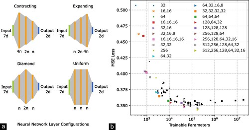
Contracting closely followed by uniform networks performed better in terms of MSE loss. In addition, deeper networks, even with smaller layer sizes, outperformed shallow networks. To understand how the models approximated the data, the expected versus predicted radial values and associated residuals per surface were plotted, see Figure 5(a and b). Networks with a limited number of parameters, for instance with one layer of 32 neurons, produced visually circular contours comprised of piece-wise continuous parabolic arcs, while deeper networks, such as the one eventually used with three layers of 128, 64, and 32 neurons, produced smoother approximations which better tracked the measured contours. Moreover, deeper networks retained subtle features, such as the over-extrusion occurring during layer-to-layer transitions, near the 0 degrees angle, and the robot's positional accuracy being higher in its Y-axis versus its X-axis motions, which can be observed by comparing the radius values about the 90, 270 versus 180 degrees angles.

Figure 5. Approximation characteristics of a simple (one layer with 32 neurons) and a complex (three layers of 128, 64, and 32 neurons) network predicting (a) the radial deformation and (b) residuals for a cylinder with 25 layers and 100 mm diameter at its 10-th layer. (c) Correction scheme iterations versus loss and (d) MSE error map for a 20-layer 100 mm diameter cylinder using the (128, 64, 32) network.

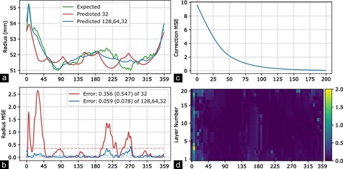
The objective of the correction scheme is to bring the exterior surface of 3D printed parts onto the desired design geometry by adjusting the extrusion machine path points. At a high level, this is accomplished by recursively updating the supplied machine path until the predicted deviation from the design is minimised. As material wall thickness varies per layer, presented in the section below, it is impossible to impose both internal and external surface constraints, without adjusting for instance the layer offsets or flow rate. In detail, a cylindrical or conic design geometry, defined as a grid of points D, is segmented into polygonal contours per layer. The initial machine path is the sequence of points P₀ = D, as the result of flattening bottom-up the grid into a list of points. Design points do not need to be offset inwards to account for the wall thickness, that is the distance from the machine path location to the exterior of the surface. The neural network is instead directly evaluated with this initially false machine path. The result is a list of displacement vectors U₀, where Q₀ = P₀ + U₀ are the predicted exterior surface points. The error vectors between the desired and predicted points V₀ = D – Q₀ are calculated. The updated machine path locations are then computed using P_i + 1 = P_i – s V_i, where s is a correction scaling factor. With each successive iteration, the initially oversized machine paths are progressively contracted. The process is repeated aiming to minimise the MSE(V) loss between the predicted and desired points, using a scaling of 0.01 over a few hundred iterations. Smaller scaling factors require more iterations while higher scaling factors produce noisy contours or even divergent behaviour. Finally, to mitigate noise among consecutive contour points [… , p_i-1, p_i, p_i + 1, …], an iterative smoothing operation, where for p_{i, j + 1} = 0.001p_{i-1, j} + 0.998p_{i, j} + 0.001p_{i + 1, j} for 10 iterations was performed. Figure 5(c) illustrates the correction loss reduction after 200 iterations for a 20-layer 100 mm diameter cylinder and the per-machine path point error map, see Figure 5(d).

Results

Shrinkage characteristics

During the drying process, capillary forces exert internal stresses resulting in substantial dimensional shrinkage, see Figure 6. Shrinkage exhibits anisotropic characteristics which may be attributed to (a) The material extrusion process itself. Specifically, material continuity differs among all principal directions, namely along the path of extrusion, in the transverse direction along the path, and vertically per layer. (b) Boundary conditions, such as at the lowest layer the material’s ability to dehydrate and shrink, is suppressed by the base plate, whereas the top layer material can dry faster being exposed to air by a larger surface fraction compared to layers below. (c) Curing physics, namely gravity-driven moisture gradients cause parts to dry top-down as well as convective drying takes place outside-in. (d) The drying regime, such as allowing artefacts to dry at ambient conditions, using fans, or curing using hot air.

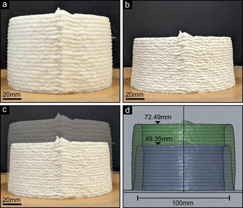
Figure 6. (a) Wet and (b) dry states of a 100 mm diameter, 20-layer cylinder, including (c) overlays of photography and (d) section view of the acquired meshes, highlighting visually the effects of shrinkage resulting in significant geometric deformation.

Change of mass m due to dehydration is substantial with m_dry / m_wet ratio of 0.245 (0.007); nearly 75% of the composite's mass evaporates. Drying at ambient temperature and relative humidity conditions takes approximately 10 days but it may be significantly reduced to three days, using convective air flow, or under 24 h using hot air, see Figure 7(a). Curing time is also affected by the nozzle diameter, for while objects 3D printed using 7 mm nozzle, require several days to cure, using 1.5 mm nozzle and forced air flow, sufficiently cures the layers deposited during 3D printing.

Figure 7. (a) Dry-to-wet mass ratio of a 100 mm diameter, 20-layer cylindrical prototype, using a 7 mm nozzle diameter, under various drying regimes. The dotted line represents normalisation to room temperature and humidity. (b) Vertical shrinkage per number of layers including both cylinders and cones of various taper angles.

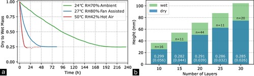
Vertical shrinkage measures the total height h difference ratio, from the base plate to the top of the print, between its wet and dry states, namely (h_wet – h_dry) / h_wet. Shrinkage among prints with a different number of layers and taper angles is overall 0.289 (0.04), which is approximately 30% height reduction, see Figure 7(b). While vertical shrinkage is the largest among all other directions, it is exactly because it is so consistent, that allows us to perform the prediction-correction scheme in 2D considering only XY-displacements. This characteristic also implies that achieving the desired height requires pre-setting the design geometry by vertical scaling and increasing the total number of layers 3D printed. The consistency of vertical shrinkage may be attributed to the compression induced by the extrusion process forcing the material from a 7 mm diameter nozzle to flatten down to 3.5 mm layer heights.

Longitudinal shrinkage (l_{wet –} l_dry) / l_wet along the extrusion path, measures the change of perimeter length l between wet and dry states. It also varies per layer, see Figure 8(a), depicting the mean sectional profile of a cylinder with a diameter of 100 mm, the perimeter length at the centre of the material run, and the per-layer shrinkage ratio. The plots highlight that the wet profiles’ centre points are close to the target 50 mm radius, see the vertical grid line. However, material extrusion pressure and compounding mass vertically introduce buckling, highlighted by the bulging shape around the 8th layer. From the dry profiles of the same cylinder, it is evident that the shape has deformed acquiring an inwards tapering profile. The trend of ramping shrinkage from the bottom layer upwards may be attributed to the effects of material adhesion at the base plate which prevents motion. Overall, longitudinal shrinkage across all layers is 0.05 (0.014). Shrinkage along the motion direction is the lowest which may be attributed to the fibre alignment induced by the extrusion process.

Figure 8. (a) Wet and dry filament perimeter lengths for a 100 mm diameter, 20-layer cylinder, and longitudinal shrinkage per layer. (b) Wet and dry filament run widths for the same cylinder and transverse shrinkage per layer.

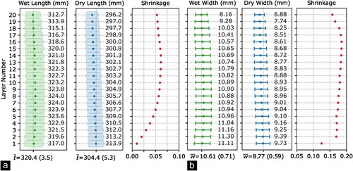
Shrinkage in the transverse direction (w_{wet –} w_dry) / w_wet, perpendicular to the direction of extrusion, expresses the change of material run-width, or wall-thickness, w between the wet and dry states. Figure 8(b), illustrates the same cylinder in section, the distances between interior and exterior surface points expressing the run-widths, and the associated wet-to-dry shrinkage per layer. It is again evident that shrinkage at the top and bottom layers is affected by the boundary conditions, namely the adhesion at the base plate, the initial 5 mm offset in contrast to 3.5 mm layer-to-layer spacing, and lower material compression of the top layers. Transverse shrinkage across all layers is 0.173 (0.013). It is exactly because the material run width varies vertically, that the prediction and correction scheme can only address either the interior or the exterior shape of the objects 3D printed.

Prediction and correction

Several corrected prototypes were 3D printed and compared with their uncorrected counterparts, see the figures below and the supplementary figures section. The procedure for creating a corrected surface involves the following steps: (a) The design surface is drawn using computer-aided design; (b) Machine paths in the form of a sequence of 3D points (n, 3) are extracted from surface contours; (c) Points are converted to (n, 7) feature vectors; (d) The model uses the entire (n, 7) tensor to compute (n, 2) displacements and the associated (n, 2) correction 2D vectors. (e) Corrections are applied, in the sense of translation, to the original machine path’s points; (f) Corrected machine path points are converted to waypoints and sent to the robot for 3D printing.

The effectiveness of the approach may be assessed by analysis of the results in terms of accuracy, namely the residuals between as-designed and as-built shapes, and precision captured by the error distribution characteristics and their standard deviation. Additionally, the taper angle of the surface profiles in the section and the roundness of the contours is also evaluated. In the section, cylindrical surfaces achieved vertical profiles, whereas they tapered if uncorrected, see Figure 9(a). The radius of the 20-layer 100 mm cylinder, for instance, is on average within 0.445 (0.298) mm from the desired 50 mm radius. The standard deviation has also significantly improved from 1.210 to 0.298. The taper angle, computed via linear regression, was corrected from −4.432 to 0.660 degrees from the vertical. The spread of errors and taper angles improved overall across all shapes tested including cylinders and cones, see Figures S2–S4.

Figure 9. Comparison of uncorrected and corrected 20-layer cylinders with 100 mm diameter. (a) Section view of profiles and distribution of errors. (b) Polar graph depicting the same cylinder in plan view.

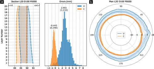
The results of the prediction-correction scheme in plan-view are presented via a polar graph of all contours, see Figure 9(b). The model successfully accounted for the offset between the machine path and the exterior surface. In addition, the model performed remarkably well in countering the over-extrusion taking place at the start and between layer-to-layer transitions. The effect is still noticeable because the machine path is segmented by a chord length of 5 mm, which allows for only a small number of correction points around the affected area to absorb the overall error. Fitting circles, in the least squares sense, per contour per layer, highlights that the standard deviation of the mean radius, a metric that hints about the roundness and noise of the shape, shows improvements from 1.106 versus 0.192, which holds, namely 1.031 and 0.147 respectively, even if the over-extrusion region points, between −45 and 45 degrees, is omitted from the regression.

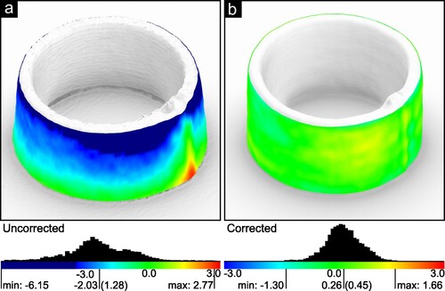
Comparing the 3D printed prototypes in relative terms, using the mean radius at the base layer, instead of the absolute target radius, see Figure 10, contextualises the distribution of errors spatially and highlights the overall shape improvement. Most errors of the corrected cylinder are circa within ±0.5 mm overall, and even the minimum and maximum error range is within approximately ±1.5 mm. This appears to be generally the case with cylinders with different numbers of layers as well as cones, see Figures S2–S4. Considering the surface roughness of the artefacts, being also within ±0.5 mm, as well as the capabilities of the 3D scanner used, namely its 0.5 mm resolution, we assess the results as satisfactory.

Figure 10. Isometric view of (a) uncorrected and (b) corrected cylinders with 20 layers and 100 mm diameter showing the relative errors from the mean base radius and distributions thereof.

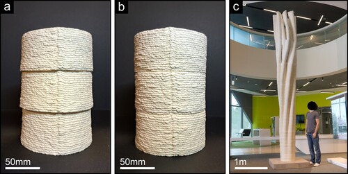
After abrasively removing the extrusion termination tail, by sanding the top surface and stacking the cured cylinders, the results may be also visually appreciated, see Figure 11(a and b). Uncorrected parts have obvious problems at the interfaces, which prevents the seamless assembly of multiple parts, while for corrected parts, transitions are less noticeable. This is an important achievement given that the time required for printing is a small fraction of the time required for curing, namely 5 min versus 72 h. Moreover, the material adheres to itself after curing, therefore logistically it makes the most sense to split larger models into smaller segments, print all thereof sequentially, cure in parallel, and finally assemble. Therefore, the overall error improvements, while they may be in the range of a few millimetres, or a small percentage of the overall diameter, their consequences are critical for such part-assembly scenarios, see Figure 11(c), for an earlier example of 5 m tall pillar design assembled from 50 uncorrected segments that motivated this work.

Figure 11. (a) Uncorrected and (b) corrected cylinders with 20 layers and 100 mm diameter stacked vertically. (c) Example of a large-scale 3D print design measuring 5 m tall, comprised of 50 segments.

Discussion

In summary, analysis of corrected 3D prints presents encouraging results with a reduction of absolute errors, with all being within one millimetre from the target, and a two to three-fold improvement of the standard deviations. For large-scale additive manufacturing applications with nozzle diameters of 7 mm and layer heights of 3.5 mm, the results achieved are satisfactory but there are also several areas for further improvement. The structured light 3D scanning equipment used, while it enabled us to rapidly capture several objects, but its low resolution became a limiting factor for further improvement. Specifically, it was difficult to accurately capture the transition from the base plate to the first layer, the ridges between layers, and the transition from the interior to the exterior surface at the top layer. Those features were smoothed by the meshing algorithm of the scanner’s software. The layers at the very bottom and top of the 3D prints are important because they exhibit atypical characteristics.

The neural networks examined here are simple compared to advanced variants such as convolutional and adversarial networks. They were employed for non-linear regression using hand-picked features. We may share a few insights that hint that perhaps it would make sense to move towards more advanced networks. The selection of features is something that the network should be able to perform by itself. It would be also preferable to directly input points from the machine path, including motion parameters, instead of computing interim geometric features. Finally, it would be certainly beneficial for the network to develop a broader understanding of the neighbourhood about a machine path point, or even the entire shape, instead of operating with exclusively local features. Those imply that convolutional networks which can detect features in higher-dimensions or recurrent networks that can incorporate transient characteristics of the 3D printing process may be applicable.

The correction scheme employs a recursion mechanism using a global scaling factor. This represents the simplest algorithm that updates the corrected model with a series of incremental contractions, marching forward up to a number of iterations or until no further improvement is possible. There are three problems with this approach: (a) Updating the last prediction compounds noise and the model diverges past the minimum instead of wandering around it, (b) Using a fixed scaling factor becomes eventually too large near the minimum, whereas an adaptive step would work better, and (c) It may be beneficial to use different scaling factor per point instead of a global one. Those point towards using the gradient descent method, employed for training the prediction model, for also addressing the correction phase. Ideally, the prediction and correction schemes are integrated such that supplying a machine path, directly produces its corrected version. Again, these hints toward more advanced neural network architectures.

Conclusions

We presented a prediction-correction scheme for compensating shrinkage and improving the geometric characteristics of cellulose-chitin biopolymers’ extrusion. The use of neural networks was effective in compensating errors both in absolute and relative terms. The model currently supports only a limited range of geometries, namely single-wall cylindrical and conic surfaces. A key challenge for expanding its scope and generality is in determining how to encode more complex features, such as the presence of material in the neighbourhood of the current machine path position. How to decouple the predictive model from absolute coordinates of the points, in the sense of achieving transformation invariance within the layer's plane. Finally, the current approach employs a prediction followed by a separate correction pass, but it would be potentially more effective to embed within the ML gradient descent optimisation scheme, not merely the prediction but also the correction phase more integrally. In conclusion, we hope that overcoming the key challenge of shrinkage in water-based biopolymer AM may enable the adoption of such environmentally benign materials for a wide range of industrial applications.

Disclosure statement

No potential conflict of interest was reported by the author(s).

Additional information

Funding

The work was supported by the Singapore MOE2018-T2-2-176 and CRP20-2017-0004 grants.

References

- Bikas, H., P. Stavropoulos, and G. Chryssolouris. 2016. “Additive Manufacturing Methods and Modelling Approaches: A Critical Review.” The International Journal of Advanced Manufacturing Technology 83 (1–4): 389–405. https://doi.org/10.1007/s00170-015-7576-2.
- Brøtan, V. 2014. “A new Method for Determining and Improving the Accuracy of a Powder bed Additive Manufacturing Machine.” The International Journal of Advanced Manufacturing Technology 74 (9–12): 1187–1195. https://doi.org/10.1007/s00170-014-6012-3.
- Chen, H., and Y. F. Zhao. 2016. “Process Parameters Optimization for Improving Surface Quality and Manufacturing Accuracy of Binder Jetting Additive Manufacturing Process.” Rapid Prototyping Journal 22 (3): 527–538. https://doi.org/10.1108/RPJ-11-2014-0149.
- Chowdhury, S., and S. Anand. 2016. “Artificial Neural Network Based Geometric Compensation for Thermal Deformation in Additive Manufacturing Processes.” Proceedings of the ASME MSEC-NAMRC. https://doi.org/10.1115/MSEC2016-8784.
- Corradini, F., and M. Silvestri. 2022. “Design and Testing of a Digital Twin for Monitoring and Quality Assessment of Material Extrusion Process.” Additive Manufacturing 51:102633. https://doi.org/10.1016/j.addma.2022.102633.
- Dastjerdi, A. A., M. R. Movahhedy, and J. Akbari. 2017. “Optimization of Process Parameters for Reducing Warpage in Selected Laser Sintering of Polymer Parts.” Additive Manufacturing 18:285–294. https://doi.org/10.1016/j.addma.2017.10.018.
- Delli, U., and S. Chang. 2018. “Automated Process Monitoring in 3D Printing Using Supervised Machine Learning.” Procedia Manufacturing 26:865–870. https://doi.org/10.1016/j.promfg.2018.07.111.
- Farhan Khan, M., A. Alam, M. Ateeb Siddiqui, M. Saad Alam, Y. Rafat, N. Salik, and I. Al-Saidan. 2021. “Real-time Defect Detection in 3D Printing Using Machine Learning.” Materials Today: Proceedings 42:521–528. https://doi.org/10.1016/j.matpr.2020.10.482.
- Goh, G. D., N. M. Bin Hamzah, and Y. Y. Wai. 2021. “Anomaly Detection in Fused Filament Fabrication Using Machine Learning.” 3D Printing and Additive Manufacturing. https://doi.org/10.1089/3dp.2021.0231.
- Guven, E., Y. Karpat, and M. Cakmakci. 2022. “Improving the Dimensional Accuracy of Micro Parts 3D Printed with Projection-based Continuous Vat Photopolymerization Using a Model-based Grayscale Optimization Method.” Additive Manufacturing 57:102954. https://doi.org/10.1016/j.addma.2022.102954.
- Hong, R., L. Zhang, J. Lifton, S. Daynes, J. Wei, S. Feih, and W. F. Lu. 2021. “Artificial Neural Network-based Geometry Compensation to Improve the Printing Accuracy of Selective Laser Melting Fabricated Sub-millimetre Overhang Trusses.” Additive Manufacturing 37:101594. https://doi.org/10.1016/j.addma.2020.101594.
- Hoo, J. L., S. Dritsas, and J. G. Fernandez. 2022. “Improving the Geometric Accuracy in Large-scale Additive Manufacturing of Fungus-like Adhesive Materials.” Proceedings Materials Today 70:603–610. https://doi.org/10.1016/j.matpr.2022.08.562.
- Huang, Q., Z. Zhang, A. T. Sabbaghi, and A. Dasgupta. 2015. “Optimal Offline Compensation of Shape Shrinkage for Three-dimensional Printing Processes.” IIE Transactions 47 (5): 431–441. https://doi.org/10.1080/0740817X.2014.955599.
- Kafara, M., J. Kemnitzer, H. H. Westermann, and R. Steinhilper. 2018. “Influence of Binder Quantity on Dimensional Accuracy and Resilience in 3D-printing.” Procedia Manufacturing 21:638–646. https://doi.org/10.1016/j.promfg.2018.02.166.
- Kakanuru, P., and K. Pochiraju. 2022. “Simulation of Shrinkage during Sintering of Additively Manufactured Silica Green Bodies.” Additive Manufacturing 56:102908. https://doi.org/10.1016/j.addma.2022.102908.
- Kim, H., H. Lee, J. S. Kim, and S. H. Ahn. 2020. “Image-based Failure Detection for Material Extrusion Process Using a Convolutional Neural Network.” The International Journal of Advanced Manufacturing Technology 111 (5–6): 1291–1302. https://doi.org/10.1007/s00170-020-06201-0.
- Kruth, J. P., M. C. Leu, and T. Nakagawa. 1998. “Progress in Additive Manufacturing and Rapid Prototyping.” Annals CIRP 47 (2): 525–540. https://doi.org/10.1016/S0007-8506(07)63240-5.
- Lee, P. H., H. Chung, S. W. Lee, J. Yoo, and J. Ko. 2014. “Review: Dimensional Accuracy in Additive Manufacturing Processes.” Proceedings of ASME V001T04A045. https://doi.org/10.1115/MSEC2014-4037.
- Liu, J., and L. Li. 2004. “In-time Motion Adjustment in Laser Cladding Manufacturing Process for Improving Dimensional Accuracy and Surface Finish of the Formed Part.” Optics and Laser Technology 36 (6): 477–483. https://doi.org/10.1016/j.optlastec.2003.12.003.
- Lynn-Charney, C., and D. Rosen. 2000. “Usage of Accuracy Models in Stereolithography Process Planning.” Rapid Prototyping 6 (2): 77–87. https://doi.org/10.1108/13552540010323600.
- Mani, M., S. Feng, B. Lane, A. Donmez, S. Moylan, and R. Fesperman. 2015. “Measurement Science Needs for Real-time Control of Additive Manufacturing Powder bed Fusion Processes.” NISTIR 8036. https://doi.org/10.6028/NIST.IR.8036.
- Mayur, V., K. Narendra, K. J. Prashant, T. Puneet, and M. P. Pulak. 2018. “Shrinkage Compensation Study for Performing Machining on Additive Manufactured Parts.” Materials Today 5 (9): 18544–18551. https://doi.org/10.1016/j.matpr.2018.06.197.
- Moroni, G., W. P. Syam, and S. Petrò. 2014. “Towards Early Estimation of Part Accuracy in Additive Manufacturing.” Procedia CIRP 21:300–305. https://doi.org/10.1016/j.procir.2014.03.194.
- Mostafaei, A., P. Rodriguez De Vecchis, I. Nettleship, and M. Chmielus. 2019. “Effect of Powder Size Distribution on Densification and Microstructural Evolution of Binder-jet 3D-Printed Alloy 625.” Materials & Design 162:375–383. https://doi.org/10.1016/j.matdes.2018.11.051.
- Muñiz Castro, B., Moe Elbadawi, J. J. Ong, T. Pollard, Z. Song, S. Gaisford, G. Pérez, A. W. Basit, P. Cabalar, and A. Goyanes. 2021. “Machine Learning Predicts 3D Printing Performance of Over 900 Drug Delivery Systems.” Journal of Controlled Release 337:530–545. https://doi.org/10.1016/j.jconrel.2021.07.046.
- Nath, P., J. D. Olson, S. Mahadevan, and Y. T. T. Lee. 2020. “Optimization of Fused Filament Fabrication Process Parameters under Uncertainty to Maximize Part Geometry Accuracy.” Additive Manufacturing 35:101331. https://doi.org/10.1016/j.addma.2020.101331.
- Noriega, A., D. Blanco, and B. J. Alvarez. 2013. “Dimensional Accuracy Improvement of FDM Square Cross-section Parts Using Artificial Neural Networks and an Optimization Algorithm.” International Journal Advanced Manufacturing Technology 69 (9–12): 2301–2313. https://doi.org/10.1007/s00170-013-5196-2.
- Osswald, A. T., J. Puentes, and J. Kattinger. 2018. “Fused Filament Fabrication Melting Model.” Additive Manufacturing 22:51–59. https://doi.org/10.1016/j.addma.2018.04.030.
- Pavan, K. G., and P. R. Srinivasa. 2014. “Multi-objective Optimisation of Strength and Volumetric Shrinkage of FDM Parts.” Virtual and Physical Prototyping 9 (2): 127–138. https://doi.org/10.1080/17452759.2014.898851.
- Rajabi, M., M. McConnell, J. Cabral, and A. M. Azam. 2021. “Chitosan Hydrogels in 3D Printing for Biomedical Applications.” Carbohydrate Polymers 260:117768. https://doi.org/10.1016/j.carbpol.2021.117768.
- Rebaioli, L., and I. Fassi. 2017. “A Review on Benchmark Artifacts for Evaluating the Geometrical Performance of Additive Manufacturing Processes.” International Journal of Advanced Manufacturing Technology 93 (5–8): 2571–2598. https://doi.org/10.1007/s00170-017-0570-0.
- Sanandiya, N. D., Y. Vijay, M. Dimopoulou, S. Dritsas, and J. G. Fernandez. 2018. “Large-scale Additive Manufacturing with Bioinspired Cellulosic Materials.” Scientific Reports 8:8642. https://doi.org/10.1038/s41598-018-26985-2.
- Soe, S. P., D. R. Eyers, and R. Setchi. 2013. “Assessment of Non-uniform Shrinkage in the Laser Sintering of Polymer Materials.” International Journal of Advanced Manufacturing Technology 68 (1–4): 111–125. https://doi.org/10.1007/s00170-012-4712-0.
- Spears, T. G., and S. A. Gold. 2016. “In-process Sensing in Selective Laser Melting (SLM) Additive Manufacturing.” Integrated Material Manufacturing Innovation 5 (1): 16–40. https://doi.org/10.1186/s40192-016-0045-4.
- Spoerk, M., J. Sapkota, G. Weingrill, T. Fischinger, F. Arbeiter, and C. Holzer. 2017. “Shrinkage and Warpage Optimization of Expanded-perlite-filled Polypropylene Composites in Extrusion-based Additive Manufacturing.” Macromolecular Material Engineering 302 (10): 1700143. https://doi.org/10.1002/mame.201700143.
- Strong, D., M. Kay, B. Conner, T. Wakefield, and G. Manogharan. 2018. “Hybrid Manufacturing – Integrating Traditional Manufacturers with Additive Manufacturing (AM) Supply Chain.” Additive Manufacturing 21:159–173. https://doi.org/10.1016/j.addma.2018.03.010.
- Tang, Y., C. Henderson, J. Muzzy, and D. Rosen. 2004. “Stereolithography Cure Modelling and Simulation.” International Journal of Material and Product Technology 21 (4): 255–272. https://doi.org/10.1504/IJMPT.2004.004941.
- Tofail, A. M. S., E. Koumoulos, A. Bandyopadhyay, S. Bose, L. O’Donoghue, and C. Charitidis. 2018. “Additive Manufacturing: Scientific and Technological Challenges, Market Uptake and Opportunities.” Materials Today 21 (1): 22–37. https://doi.org/10.1016/j.mattod.2017.07.001.
- Tong, K., S. Joshi, and E. Lehtihet. 2008. “Error Compensation for Fused Deposition Modelling (FDM) Machine by Correcting Slice files.” Rapid Prototyping Journal 14 (1): 4–14. https://doi.org/10.1108/13552540810841517.
- Turner, B. N., and S. A. Gold. 2015. “A Review of Melt Extrusion Additive Manufacturing Processes: II. Materials, Dimensional Accuracy, and Surface Roughness.” Rapid Prototyping Journal 21 (3): 250–261. https://doi.org/10.1108/RPJ-02-2013-0017.
- Vijay, Y., N. D. Sanadiya, S. Dritsas, and J. G. Fernandez. 2019. “Control of Process Settings for Large-scale Additive Manufacturing with Sustainable Natural Composites.” Journal of Mechanical Design 141 (8): 081701. https://doi.org/10.1115/1.4042624.
- Yang, Y., D. McGregor, S. Tawfick, W. King, and C. Shao. 2022. “Hierarchical Data Models Improve the Accuracy of Feature Level Predictions for Additively Manufactured Parts.” Additive Manufacturing 51:102621. https://doi.org/10.1016/j.addma.2022.102621.
- Zago, M., F. M. Lecis, M. Vedani, and I. Cristofolini. 2021. “Dimensional and Geometrical Precision of Parts Produced by Binder Jetting Process as Affected by the Anisotropic Shrinkage on Sintering.” Additive Manufacturing 43:102007. https://doi.org/10.1016/j.addma.2021.102007.