
 ?Mathematical formulae have been encoded as MathML and are displayed in this HTML version using MathJax in order to improve their display. Uncheck the box to turn MathJax off. This feature requires Javascript. Click on a formula to zoom.
Abstract
We answer the question how arbitrarily small perturbations of a pair of one arbitrary and one symmetric matrix can change a normal form with respect to a certain linear group action. This result is then applied to describe the quadratic part of normal forms of complex points of small
-perturbations of real 4-manifolds embedded in a complex 3-manifold.
1. Introduction
The study of complex points was started in 1965 by E. Bishop with his seminal work on the problem of describing the hull of holomorphy of a submanifold near a point with one-dimensional complex tangent space [Citation1]. This is now very well understood for surfaces (see Bishop [Citation1], Kenig and Webster [Citation2], Moser and Webster [Citation3]), and it later initiated in many researches in geometric analysis. For instance, (formal) normal forms for real submanifolds in near complex points were considered by Burcea [Citation4], Coffman [Citation5], Gong [Citation6], Gong and Stolovich [Citation7], Moser and Webster [Citation3] among others. We add that topological structure of complex points was first considered by Lai [Citation8] and in the special case of surfaces by Forstnerič [Citation9]. Up to
-small isotopy complex points of real codimension 2 submanifolds in complex manifolds were treated by Slapar [Citation10–12].
In this paper we describe the behavior of the quadratic part of normal forms of complex points of small -perturbations of real 4-manifolds embedded in a complex 3-manifold (see Corollary 3.8). It is a direct consequence of a result that clarifies how a normal form for a pair of one arbitrary and one symmetric
matrix with respect to a certain linear algebraic group action changes under small perturbations (see Theorem 3.6); by a careful analysis we also provide information how small the perturbations must be. Due to technical reasons, these results are precisely stated in Section 3 and then proved in later sections.
Let be a
-smooth embedding of a real smooth
-manifold into a complex
-manifold
. A point
is CR-regular if the dimension of the complex tangent space
is n−1, while p is called complex when the complex dimension of
equals n, thus
. By Thom's transversality theorem [Citation13, Section 29], for generic embeddings the intersection is transverse and so complex points are isolated. Using Taylor expansion M can near a complex point
be seen as a graph:
where
are suitable local coordinates on X, and
,
,
. By
we denote the group of all
complex matrices, and by
,
, respectively, its subgroups of symmetric and nonsingular matrices. After a simple change of coordinates
it is achieved that
, and the normal form up to quadratic terms is:
(1)
(1) A real analytic complex point p is called flat, if local coordinates can be chosen so that the graph (Equation1
(1)
(1) ) lies in
. It is quadratically flat, if the quadratic part of (Equation1
(1)
(1) ) is real valued; this happens precisely when A in (Equation1
(1)
(1) ) is Hermitian.
Any holomorphic change of coordinates that preserves and
as a set in (Equation1
(1)
(1) ), has the same effect on the quadratic part as a complex-linear change
Furthermore, using this linear changes of coordinates and a biholomorphic change
transforms (Equation1
(1)
(1) ) into the equation that can by a slight abuse of notation be written as
Studying the quadratic part of complex points thus means examining the action of a linear group
on pairs of matrices
, introduced in [Citation5]:
(2)
(2) Problems of the quadratic part thus reduce to problems in matrix theory.
When n = 1 complex points are always quadratically flat and locally given by the equations ,
or
(Bishop [Citation1]). If in addition they are real analytic and elliptic (
), they are also flat (see [Citation3]). A relatively simple description of normal forms of the action (Equation2
(2)
(2) ) was obtained for n = 2 (see Coffman [Citation5] and Izotov [Citation14]), while in dimensions 3 and 4 a complete list of normal forms has been given only in the case of quadratically flat complex points (see Slapar and Starčič [Citation15]). Nevertheless, if B in (Equation1
(1)
(1) ) is nonsingular the classification has been done even in higher dimensions by the result of Hong [Citation16].
The problem of normal forms of matrices under perturbations was first studied by Arnold (see e.g. [Citation13]), who considered matrices depending on parameters under similarity (miniversal deformations). The change of Jordan canonical form has been then successfully investigated through the works of Markus and Parilis [Citation17], Edelman, Elmroth and Kågstrom [Citation18], among others; the software Stratigraph [Citation19] constructs the relations between Jordan forms. However, the problem of normal forms for -conjugation (or T-conjugation) under small perturbations seems to be much more involved, and has been so far inspected only in lower dimensions; check the papers Futorny, Klimenko and Sergeichuk [Citation20], Dmytryshyn, Futorny and Sergeichuk [Citation21] (Dmytryshyn, Futorny, Kågström, Klimenko and Sergeichuk [Citation22]). Virtually nothing has been known until the time of this writing about simultaneous small perturbations of pairs of matrices under these actions.
In connection to these problems we mention results of Guralnick [Citation23] and Leiterer [Citation24], who respectively studied similarity of holomorphic maps from Riemann surfaces or Stein spaces to a set of matrices. We shall not consider this matter here.
2. Normal forms in dimension 2
We recall the basic properties of an action of a Lie group on a manifold (check e.g. [Citation25, Theorem IV.9.3]). These are well known and they are not difficult to prove.
Proposition 2.1
Let be a smooth
analytic
action of a real
complex
Lie group G with a unit e, acting on a smooth
complex
manifold X, i.e.
Then Φ satisfies the following properties:
For any
the map
For any
An orbit of
Any orbit can be endowed (globally) with the structure of a manifold, but it does not necessarily coincide with the subspace topology [Citation25, Theorem IV.9.6].
We proceed with the list of representatives of orbits (normal forms) of the action (Equation2(2)
(2) ) for n = 2 obtained by Coffman (see [Citation5, Section 7,Table 1]). In addition, we compute tangent spaces of orbits and then arrange normal forms into a table according to dimensions of their orbits (42 types); these are calculated similarly as in the case of similarity (see e.g. Arnold [Citation13, Section 30]). To simplify the notation,
denotes the diagonal matrix with a, d on the main diagonal, while the
identity-matrix and the
zero-matrix are
and
, respectively.
Lemma 2.2
Orbits of the action (Equation2(2)
(2) ) for n = 2 are immersed manifolds, they are represented by its normal forms
given in Table
the dimensions are noted in the first column
.
Table 1. Orbits of the action (Equation2(2) (2) ) for n = 2.
A minor change is made in comparison to the original list in [Citation5], as is taken instead of
; conjugate the later one with
.
Proof
Proof of Lemma 2.2
By Proposition 2.1 (2), (3), orbits of the action Ξ in (Equation2(2)
(2) ) for n = 2 are immersed manifolds. To compute the tangent space of the orbit
we fix
, choose a path going through
:
and then calculate
Writing
,
, where
is the elementary matrix with one in the jth row and kth column and zeros otherwise, we deduce that
and in a similar fashion we conclude that
Let a
complex (symmetric) matrix be identified with a vector in a real Euclidean space
(and
), thus
with the standard basis
. The tangent space of an orbit
can then be seen as the linear space spanned by the vectors
, where
(3)
(3)
We split our consideration of tangent spaces according to the list of normal forms in [Citation5, Section 7,Table 1] into several cases. In each case the tangent space will be written as a direct sum of linear subspaces (with trivial intersection) such that
and
will be either trivial or its vectors will be of the form
with some nonvanishing
,
.
Case I. ,
,
From (Equation3(3)
(3) ) we obtain that
It is apparent that
. By further setting
we can choose
,
and observe that
.
Case II. ,
,
,
We have (see (Equation3(3)
(3) )):
It is immediate that
.
For we set
,
and we have
and
. Next, for
,
we take
and
with
,
.
Finally, for we set
If we choose
,
, then
,
.
Case III. ,
,
,
It follows from (Equation3(3)
(3) ) that
Let us denote
For 0<t<1 we set
,
and get that
,
. Next, if t = 1 we take
,
. Observe that
,
. Finally, when t = 0 we set
(4)
(4) with
,
. It follows that
and
.
Case IV . ,
,
By (Equation3(3)
(3) ) we have
These vectors are contained in
and
,
. It is now easy to compute the dimension of their linear span.
This finishes the proof.
Remark 2.3
Sometimes it it is more informative to understand the stratification into bundles of matrices, i.e. sets of matrices having similar properties. Again, this notion was introduced first by Arnold [Citation13, Section 30]. Given a parameter set Λ with smooth maps ,
, one considers a bundle of pairs of matrices under the action Ξ in (Equation2
(2)
(2) ), i.e. a union of orbits
. We set
(5)
(5) and observe that for any
we have
. In a similar manner as we computed the tangent space of an orbit, the tangent space of a bundle can be obtained. It follows that the generic
pairs of one arbitrary and one symmetric matrix (forming a bundle with maximal dimension 14) under the action (Equation2
(2)
(2) ) for n = 2 are:
Indeed, tangent spaces of these bundles are spanned by the tangent vectors in Case II and Case III of the proof of Lemma 2.2 (for the appropriate parameters).
Note that using the list of normal forms in dimension 2, recently a result on holomorphical flattenability of CR-nonminimal codimension 2 real analytic submanifold near a complex point in ,
, was obtained through the works of Huang and Yin [Citation26, Citation27], Fang and Huang [Citation28].
3. Change of the normal form under small perturbations
In this section we study how small deformations of a pair of one arbitrary and one symmetric matrix can change its orbit under the action (Equation2(2)
(2) ) for n = 2.
First recall that ,
are in the same orbit with respect to the action (Equation2
(2)
(2) ) if and only if there exist
,
such that
. By real scaling P we can assume that
, and after additional scaling P by
we eliminate the constant
. Thus the orbits of the action (Equation2
(2)
(2) ) are precisely the orbits of the action of
acting on
by:
(6)
(6) The projections are smooth actions as well:
(7)
(7)
(8)
(8)
Next, let
,
be in the same orbit under the action (Equation6
(6)
(6) ) (
,
for some
,
) and let
be a perturbation of
:
A suitable perturbation of
is in the orbit of an arbitrarily chosen perturbation of
. It is thus sufficient to consider perturbations of normal forms.
Observe further that an arbitrarily small perturbation of is contained in
if and only if
(and hence the whole orbit
) is contained in the closure of
. The same conclusion also holds for actions
,
.
For the sake of clarity the notion of a closure graph for an action has been introduced. Given an action Φ, the vertices in a closure graph for Φ are the orbits under Φ, and there is an edge (a path) from a vertex (an orbit) to a vertex (an orbit)
precisely when
lies in the closure of
. The path from
to
is denoted briefly by
. There are few evident properties of closure graphs:
For every vertex
Paths
If there is no path from
To simplify the notation , we usually write
, where
,
. In case
it is useful to know the distance of
from the orbit of V. We shall use the standard max norm
,
to measure the distance between two matrices. This norm is not submultiplicative, but
(see [Citation29, p. 342]).
Proceed with basic properties of closure graph for the actions (Equation6(6)
(6) ), (Equation7
(7)
(7) ), (Equation8
(8)
(8) ).
Lemma 3.1
Suppose
and
.
There exists a path
The existence of a path
If
If
There exists a path
When
If
Proof.
By definition (
) if and only if
(
) for some
(
). It is equivalent to (Equation9
(9)
(9) ) (see (Equation7
(7)
(7) ), (Equation8
(8)
(8) )), so the first part of (1) is proved. Apparently,
is then equivalent to (Equation10
(10)
(10) ).
Since the orbit map of the action (the action
) is by Lemma 2.1 (2) of constant rank and hence locally a submersion (see e.g. [Citation25, Theorem II.7.1]), this action has the so-called local Lipschitz property, i.e. if A,
(B,
) are sufficiently close and
(
), then P can be chosen near to identity and c near 1. For any sufficiently small E (or F) such that
,
(
,
) are in the same orbit, then there exists some P close to the identity-matrix and c close to 1, so that
is equal to
(equal to
). As the inverse map
is continuous,
is close to identity-matrix, too. Hence
is in the orbit of
(or
), where
(
) is arbitrarily close to the zero-matrix. This concludes the proof of the first part of (2).
Next, applying the determinant to (Equation9(9)
(9) ) we get
(11)
(11) for some
,
(
). This implies (1) (a) (i).
A necessary condition for to be in the closure of
is that
and
are in the closures of
and
, respectively. Further, by multiplying the limits in (Equation11
(11)
(11) ) for
by
or
, and by comparing the absolute values of the expressions, we deduce (2) (a) (i).
It is well known that the distance from a nonsingular matrix X to the nearest singular matrix with respect to the norm is equal to
(see e.g. [Citation29, Problem 5.6.P47]). Thus (1) (b) follows. Next, applying the triangle inequality, estimating the absolute values of the entries of the matrices by the max norm of the matrices, and by slightly simplifying, we obtain for
:
(12)
(12) Let
, B,
, A be nonsingular matrices,
Using (Equation12
(12)
(12) ) for
, D = E and
, D = F with
, respectively, we get
(13)
(13)
(14)
(14)
To estimate the left-hand sides of the above inequalities from above by
it suffices to take
and
. By combining (Equation13
(13)
(13) ), (Equation14
(14)
(14) ) and applying the triangle inequality we then conclude
By (2) (a) (i) (already proved) we have
and this gives (2) (b).
It is left to show the orbit-dimension inequalities (1) (a) (ii) and (2) (a) (ii). Since orbits of Ψ, ,
can be seen as nonsingular algebraic subsets in Euclidean space (zero loci of polynomials), these facts can be deduced by using a few classical results in real (complex) algebraic geometry [Citation30, Propositions 2.8.13,2.8.14] (or [[Citation31, Propositions 21.4.3,21.4.5], [Citation32, Exercise 14.1.]]). Indeed, orbits
,
,
are contained in the closures (also with respect to a coarser Zariski topology) of orbits
,
,
, respectively. Hence algebraic dimensions of orbits mentioned first are strictly smaller than algebraic dimensions of the later orbits. Finally, orbits are locally regular submanifolds and their manifold dimensions agree with their algebraic dimensions.
Remark 3.2
Lemma 3.1 provides a quantitative information on the distance from an element to another orbit. We observe that it suffices to consider only normal forms. Given any the induced operator norms of maps
,
and
,
are bounded from above by
and
, respectively. If
,
are in the same orbit (i.e.
,
with
,
), then for any
,
we get:
When inspecting
where either A,
or B,
are in the same orbit and sufficiently close, it is by (2) enough to analyse perturbations of the matrix
(the matrix
). Unfortunately, we do not know how close the matrices should be since the constant rank theorem (even the quantitative version [Citation33, Theorem 2.9.4]) does not provide the size of the local charts which define the orbits.
By Autonne-Takagi factorization (see e.g. [Citation29, Corolarry 4.4.4]), any complex symmetric matrix is unitary T-congruent to a diagonal matrix with non-negative diagonal entries, hence T-congruent to a diagonal matrix with ones and zeros on the diagonal. Therefore symmetric matrices with respect to T-conjugacy consist of three orbits, each containing matrices of the same rank. Their closure graph is thus very simple. (For closure graphs of all
or
matrices see [Citation20].)
Lemma 3.3
The closure graph for the action (Equation8(8)
(8) )
-conjugacy on
is
where
. Moreover, if
B are vertices in the above graph, and such
with
for some
then
.
The (non)existence of most paths in the closure graph for the action in (Equation7
(7)
(7) ) follows immediately from the (non)existence of paths in the closure graph for
-conjugacy [Citation22, Theorem 2.2]. The remaining paths are treated by a slight adaptation of the
-conjugacy case. By a careful analysis we provide necessary (sufficient) conditions for the existing paths; see Lemma 3.4 (its proof is given in Section 4). These turn out to be essential in the proof of Theorem 3.6. Furthermore, if
we find a lower bound for the distance from
to
. Note that normal forms for
were first observed by Coffman [Citation34, Theorem 4.3], and by calculating their stabilizers eventually normal forms for the action (Equation6
(6)
(6) ) were obtained [Citation5, Subsection 2.4].
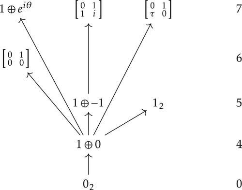
Lemma 3.4
The closure graph for the action (Equation7(7)
(7) ) is drawn in Figure . It contains an infinite set of vertices corresponding to the orbits with normal forms
indexed by the parameters θ, τ
respectively.
Figure 1. The closure graph for the action (Equation7(7)
(7) );
,
. (Orbits at the same horizontal level have the same dimension and these are indicated on the right.)
Furthermore, let A be normal forms in Figure , and let
for some
. Then one of the following statements holds:
If
If
Table 2. Given , , , , the moduli of the expressions listed in the fourth column are bounded from above by . (The constant depends only on A, .)
Remark 3.5
Constants μ or ν in Lemma 3.4 are calculated for any given pair (see Lemma 3.1 and the proof of Lemma 3.4). The existence of the constant ρ (computable as well) in the converse in Lemma 3.4 (2) is showed only in those cases where it turns to be useful in the proof of Theorem 3.6, though it is expected to be proved (possibly by a slight modification) for most of the cases.
We are ready to state the main results of the paper. The following theorem describes the closure graph for the action (Equation6(6)
(6) ). Its proof is given in Section 5. It is expected that by adapting the proof a similar result should hold for the restriction of the action (Equation6
(6)
(6) ) with c = 1; in this case there are few more types of orbits.
Theorem 3.6
Orbits with normal forms from Lemma 2.2 are vertices in the closure graph for the action (Equation6(6)
(6) ). The graph has the following properties:
There is a path from
There exist paths from
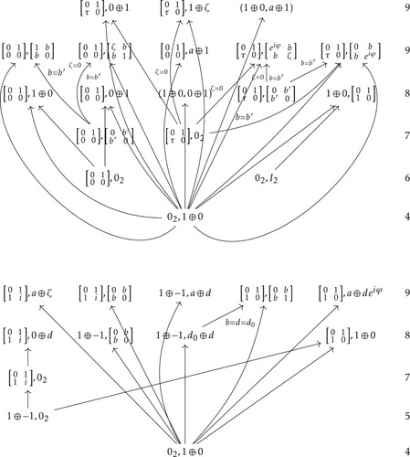
All nontrivial paths
Figure 2. All nontrivial paths with nontrivial
for
in the closure graph for the action (Equation6
(6)
(6) ). The dimensions of orbits are indicated on the right.
Remark 3.7
If in the closure graph for the action (Equation6
(6)
(6) ), it is possible to give some lower bound for the distance from
to the orbit of
; this bound will be provided as part of the proof of Theorem 3.6 in Section 5. However, it makes the proof of the theorem much longer and more involved. One must work with inequalities instead of inspecting the convergence of sequences (see Lemma 3.1), hence many intrigueing and sometimes tedious estimates need to be done. Note also that the non-existence of certain paths in the closure graph (sometimes with a bound for the distances) follow already from Lemmas 3.3, 3.4 and 3.1 (a) (2) (i), (ii).
It would be interesting to have the closure graph for bundles of matrices with respect to the action (Equation6(6)
(6) ) (see (Equation5
(5)
(5) )) or its restriction. One would need to consider the same equations as in our case, but possibly with less constraints.
Let M be a compact codimension 2 submanifold in a complex manifold X. Since the complex dimension of the complex tangent spaces near a regular point of M is preserved under small perturbations, complex points of a small deformation of M can arise only near complex points of M. Recall that
(a normal form up to quadratic terms) can be associated to a complex point
, so that in a neighborhood of p the submanifold M is of the form (Equation1
(1)
(1) ) for
,
. If
is a
-small deformation of M, then it is seen near p as a graph:
where
are local coordinates with
,
,
small, and
,
close to
,
, respectively. Similarly as in the exposition in Section 1 a complex point on this graph is put into the standard position (Equation1
(1)
(1) ) for
,
. (Translate the complex point to
, use a complex-linear transformation close to identity to insure the tangent space at
to be
, and finally eliminate z-terms.) The next result is hence a direct consequence of Theorem 3.6.
Corollary 3.8
Let M be a compact real 4-manifold embedded -smoothly in a complex 3-manifold X and let
be its isolated complex points with the corresponding normal forms up to quadratic terms
. Assume further that
is a deformation of M obtained by a smooth isotopy of M, and let
be a complex point with the corresponding normal form up to quadratic terms
. If the isotopy is sufficiently
-small then p is arbitrarily close to some
and there is a path
in the closure graph for the action (Equation6
(6)
(6) ).
Remark 3.9
In the proof of Theorem 3.6 the lower estimates for the distances from normal forms to other orbits are provided, therefore it can be told how small the isotopy (of M) in the assumption of Corollary 3.8 needs to be.
4. Proof of Lemma 3.4
In this section we prove Lemma 3.4. We start with the following technical lemma related to actions (Equation7(7)
(7) ) and (Equation8
(8)
(8) ).
Lemma 4.1
Suppose
If
Proof.
First, we observe the following simple fact. For :
(19)
(19) Indeed, we have
with
, hence
and
.
Next, the right-hand side of (Equation12(12)
(12) ) leads to
(20)
(20) By assuming
and applying (Equation19
(19)
(19) ) to (Equation20
(20)
(20) ) we obtain
(21)
(21) We apply
to
,
and after simplifying we get
(22)
(22) From (Equation21
(21)
(21) ) for
, D = E and (Equation22
(22)
(22) ) it follows that
,
,
with ψ as in (Equation21
(21)
(21) ) with
, D = E. Using well known facts
and
for
, we deduce (Equation16
(16)
(16) ). Furthermore, (Equation20
(20)
(20) ) for
, D = E and (Equation22
(22)
(22) ) for
, D = F give
(23)
(23) respectively. To conclude the proof we observe another simple fact. If
then
(24)
(24) To see this, we take
to be the square root of 1 + s (thus
) with
and
. It yields
. For
and
(
in (Equation23
(23)
(23) )), we apply (Equation24
(24)
(24) ) to (Equation23
(23)
(23) ) for s = p and s = q, respectively. It implies (Equation17
(17)
(17) ) and (2).
Proof
Proof of Lemma 3.4
For actions Ψ, (see (Equation6
(6)
(6) ) and (Equation7
(7)
(7) )), it follows that
if and only if
and
. Hence
, where dimensions of orbits of
are obtained from Lemma 2.2.
To prove it is sufficient to find
,
such that
(25)
(25) It is straightforward to see that
with
in (Equation25
(25)
(25) ) yields
, while to prove
,
, and
, we take
and
, respectively, and in both cases again with
. (Compositions of these paths represent paths as well.) It is then left to find necessary (sufficient) conditions for the existence of these paths, i.e. given A,
, E satisfying
(26)
(26) we must find out how c, P depend on E (how E depends on c, P).
On the other hand, if (Equation26(26)
(26) ) fails for every sufficiently small E, it gives
. To prove (1), upper estimates for
will be provided in such cases. This has already been done for
, A = 0 and
,
(see Lemma 3.1 (1) (i)).
Throughout the rest of the proof we denote
(27)
(27) and split our consideration of the remaining paths
into several cases.
Case I. It is straightforward to compute
Multiplying Equations (Equation26
(26)
(26) ) by
and then writing them componentwise yields
(28)
(28) The real and the imaginary parts of the first and the last equation of (Equation28
(28)
(28) ) give:
(29)
(29) while by adding (subtracting) the second and the complex-conjugated third equation of (Equation28
(28)
(28) ) for
we deduce
(30)
(30)
For
If
The first and the last equation of (Equation28
respectively. Next, from (Equation30
Thus the first part of (2) for (C4) follows; the converse is immediate by (Equation28
By (Equation16
Observe that for
After multiplying the third and the fifth equation of (Equation32
Combining it with (Equation31
The statement (2) for (C6) follows immediately from (Equation32
Case II. ,
We have
Thus (Equation26(26)
(26) ) multiplied by
and written componentwise (also rearranged) yields:
(34)
(34) Subtracting the second complex-conjugated equation (and multiplied by λ) from the third equation (and multiplied by
) for
further gives
(35)
(35)
By taking the imaginary and the real parts ob the first and the last equation of (Equation34
If
It is left to consider
Applying the triangle inequality to the second equation of (Equation34
By (Equation16
Finally, for
Applying these estimates to the second equation of (Equation34
If
The second (third) equation of (Equation34
By (Equation16
We now take the imaginary parts of Equations (Equation38
Next, let
If
Case III. ,
We calculate
Thus (Equation26
(26)
(26) ) multiplied by
and rearranged is equivalent to
(42)
(42) Rearranging the terms of the first and the last equation immediately yields
(43)
(43) while multiplying the third (second) complex-conjugated equation with τ, subtracting it from the second (third) equation, and rearranging the terms, give
(44)
(44)
Since
Conversely, we assume that the expressions (C3) for
From (Equation43
Equations (Equation44
By (Equation16
From (Equation44
This completes the proof of the lemma.
5. Proof of Theorem 3.6
Proof
Proof of Theorem 3.6
Recall that the existence of a path in the closure graph for the action (Equation6
(6)
(6) ), immediately implies (see Lemma 3.1):
(51)
(51) When any of the conditions (Equation51
(51)
(51) ) is not fulfilled, then
and we already have a lower estimate on the distance from
to the orbit of
(see Lemmas 3.1, 3.3, 3.4). Further,
if and only if
, and trivially
for any A, B.
From now on we suppose ,
, and such that (Equation51
(51)
(51) ) is valid. Let
(52)
(52) Due to Lemmas 3.4, 4.1 the first equation of (Equation52
(52)
(52) ) yields the restrictions on P, c imposed by
. Using these we then analyse the second equation of (Equation52
(52)
(52) ). When it implies an inequality that fails for any sufficiently small E, F, it proves
. The inequality just mentioned also provides the estimates how small E, F should be; this calculation is very straightforward but is often omitted.
On the other hand, if given matrices A, B, ,
we can choose E and F in (Equation52
(52)
(52) ) to be arbitrarily small, this will yield
. In most cases we find
,
such that
(53)
(53) However, to confirm the existence of a path we can also prove the existence of suitable solutions of (Equation52
(52)
(52) ) by using the last part of Lemma 3.4 (2).
Throughout the rest of the proof we denote (the constant
is provided by Lemma 3.4),
,
where sometimes polar coordinates for x, y, u, v in P might be preferred:
(54)
(54) The second matrix equation of (Equation52
(52)
(52) ) can thus be written componentwise as:
(55)
(55) For the sake of simplicity some estimates in the proof are crude, and it is always assumed
. When applying Lemma 4.1 with
or
nonsingular we in addition take
or
, respectively. Furthermore, we use the notation
when the existence of a path is yet to be considered.
We split our analysis into several cases. (For normal forms recall Lemma 2.2.)
Case I. ,
,
Denoting ,
and slightly rearranging the terms in (Equation55
(55)
(55) ) yields
(56)
(56) From Lemma 3.4 (2) for (C5) we get
and
(therefore
,
). By applying the triangle inequality we conclude from the first equation of (Equation56
(56)
(56) ) that
and similarly the last two equations of (Equation56
(56)
(56) ) yield
Since
, a comparison of the left-hand and the right-hand sides of the above inequalities implies that at least one of them fails for
such that
Case II. ,
From Lemma 3.4 (2) for (C8) for ,
we have
(57)
(57)
From (Equation55
Applying the triangle inequality to (Equation58
Using the notation (Equation54
From (Equation55
From (Equation55
Case III. ,
,
It is easy to check that and
with
in (Equation53
(53)
(53) ) prove
and
, respectively.
By Lemma 3.4 (2) for (C7) we have
(67)
(67) Set
,
,
and after rearranging the terms we write (Equation55
(55)
(55) ) as
(68)
(68)
. Applying the triangle inequality to the second equation gives
(69)
(69) Next, multiplying
and
with
(see (Equation67
(67)
(67) )) gives
and
, respectively (recall
). Thus either
or
or
,
(or more of them) are bounded by
.
From (Equation67
We deal with this case in the same manner as in Case III (a), we only replace
Here the inequality (Equation69
First, let
For
Next, let
From (Equation71
Case IV .
Lemma 3.4 (2) with (C6) for ,
,
, k = 0 (since
) gives
(74)
(74)
From (Equation55
We have the same equations as in (Equation63
By slightly rearranging the terms in (Equation55
a = 0 or
If a = 0,
Inequalities (Equation75
If
The first equation of (Equation58
Case V .
From Lemma 3.4 (2) with (C6) for ,
we obtain
(77)
(77)
For
We have the same equations as in (Equation58
We have Equations (Equation65
The first equation of (Equation55
The first and the last equation of (Equation63
Case VI.
Lemma 3.4 (2) with (C6) for ,
yields
(78)
(78)
Setting
Since
From (Equation55
Case VII.
Lemma 3.4 (2) with (C3) for ,
gives
(82)
(82) with
.
First, consider
For
From (Equation55
The first and the last equation of (Equation84
If uv = 0, then (Equation84
For
From (Equation55
The first (the second) equation of (Equation82
The first two equations of (Equation82
Case VIII.
Lemma 3.4 (2) for (C10) gives
(91)
(91)
We have Equation (Equation58
Next, let a = d. By combining (Equation61
Combining the first and the last equality of (Equation91
The first equation of (Equation79
The same proof as in Case VI (b) (ii) works here, too.
We consider
Case IX. ,
(see Lemma 2.2 and (Equation51
(51)
(51) ))
Lemma 3.4 (2) with (C3) for ,
and with some
gives
(93)
(93)
Due to the second equation of (Equation87
It is clear that either
We write the first and the last equality of (Equation93
First, let
If v = 0, then (Equation87
In this case it is convenient to conjugate
Similarly as in (Equation94
We have Equation (Equation84
Case X.
For
From Lemma 3.4 (2) with (C4) for
When
To prove
We prove
By Lemma 3.4 (2) for (C2) with
Case XI.
From Lemma 3.4 (2) with (C9) for we get that
(95)
(95)
The first equation of (Equation63
From (Equation55
When
Finally,
We have
Case XII.
By Lemma 3.4 (2) for (C1) we have
Next, let
Next, we observe the range of the function
Provided that
Furthermore
From Lemma 3.4 (2) for (C8) for
We take
Case XIII.
Lemma 3.4 (2) for (C3) for
From the first estimate in (Equation101
To prove the existence of a path for any
In view of the notation (Equation54
Let x, u be as in (Equation54
To prove the existence of a path we use the same argument as in Case XIII (a) (ii). For a given s>0 it suffices to solve the equations
It is equivalent to consider
When
Case XIV .
From Lemma 3.4 (2) for (C2) with
From (Equation109
If
Next, if
As in Case XII (a) we argue that (Equation52
Observe that since
Set
Denoting further x, y, u, v as in (Equation54
If
Since
If a = d = 0 the second equation of (Equation110
Next, suppose
If
Finally, let
Case XV .
If
Next, let
We have Equation (Equation58
In case d = 0,
Next, let a = 0 (hence d>0). The first equation of (Equation58
It is left to consider the case a>0,
Thic completes the proof of the theorem.
Acknowledgments
The author wishes to thank M. Slapar for helpful discussions considering the topic of the paper.
Disclosure statement
No potential conflict of interest was reported by the authors.
Additional information
Funding
References
- Bishop E. Differential manifolds in complex Euclidean space. Duke Math J. 1965;32:1–21. doi: 10.1215/S0012-7094-65-03201-1
- Kenig CE, Webster SM. The local hull of holomorphy of a surface in the space of two complex variables. Invent Math. 1982;67(1):1–21. doi: 10.1007/BF01393370
- Moser JK, Webster SM. Normal forms for real surfaces in C2 near complex tangents and hyperbolic surface transformations. Acta Math. 1983;150(3–4):255–296. doi: 10.1007/BF02392973
- Burcea V. A normal form for a real 2-codimensional submanifold in CN+1 near a CR singularity. Adv Math. 2013;243:262–295. doi: 10.1016/j.aim.2013.04.018
- Coffman A. CR singularities of real fourfolds in C3. Illinois J Math. 2009;53(3):939–981. doi: 10.1215/ijm/1286212924
- Gong X. Real analytic submanifolds under unimodular transformations. Proc Amer Math Soc. 1995;123(1):191–200. doi: 10.1090/S0002-9939-1995-1231299-8
- Gong X, Stolovitch L. Real submanifolds of maximum complex tangent space at a CR singular point I. Invent Math. 2016;206(1):293–377. doi: 10.1007/s00222-016-0654-8
- Lai HF. Characteristic classes of real manifolds immersed in complex manifolds. Trans AMS. 1972;172:1–33. doi: 10.1090/S0002-9947-1972-0314066-8
- Forstnerič F. Complex tangents of real surfaces in complex surfaces. Duke Math J. 1992;67(2):353–376. doi: 10.1215/S0012-7094-92-06713-5
- Slapar M. Cancelling complex points in codimension 2. Bull Aus Math Soc. 2013;88(1):64–69. doi: 10.1017/S0004972712000652
- Slapar M. Modeling complex points up to isotopy. J Geom Anal. 2013;23(4):1932–1943. doi: 10.1007/s12220-012-9312-6
- Slapar M. On complex points of codimension 2 submanifolds. J Geom Anal. 2016;26(1):206–219. doi: 10.1007/s12220-014-9545-7
- Arnold VI. Geometric methods in the theory or ordinary differential equations. New York (NY): Springer-Verlag; 1988.
- Izotov GE. Simultaneous reduction of a quadratic and a Hermitian form. Izv Vysš Učebn Zaved Matematika. 1957;1:143–159.
- Slapar M, Starčič T. On normal forms of complex points of codimension 2 submanifolds. J Math Anal Appl. 2018;461(2):1308–1326. doi: 10.1016/j.jmaa.2018.01.039
- Hong Y. A canonical form for Hermitian matrices under complex orthogonal congruence. SIAM J Matrix Anal Appl. 1989;10(2):233–243. doi: 10.1137/0610018
- Markus AS, Parilis EÉ. The change of the Jordan structure of a matrix under small perturbations. Mat Issled. 1980;54:98–109. English translation: Linear Algebra Appl. 1983;54:139–152.
- Edelman E, Elmroth E, Kågström B. A geometric approach to perturbation theory of matrices and matrix pencils. Part II: A stratification enhanced staircase algorithm. SIAM J Matrix Anal Appl. 1999;20:667–699. doi: 10.1137/S0895479896310184
- Elmroth E, Johansson P, Kågström B. Computation and presentation of graph displaying closure hierarchies of Jordan and Kronecker structures. Numer Linear Algebra Appl. 2001;8:381–399. doi: 10.1002/nla.253
- Dmytryshyn AR, Futorny V, Kågström B, et al. Change of the congruence canonical form of 2-by-2 and 3-by-3 matrices under perturbations and bundles of matrices under congruence. Linear Algebra Appl. 2015;469:305–334. doi: 10.1016/j.laa.2014.11.004
- Dmytryshyn AR, Futorny V, Sergeichuk VV. Miniversal deformations of matrices of bilinear forms. Liner Algebra Appl. 2012;436:2670–2700. doi: 10.1016/j.laa.2011.11.010
- Futorny V, Klimenko L, Sergeichuk VV. Change of the ∗-congruence canonical form of 2-by-2 matrices under perturbations. Electr J Lin Alg. 2014;27:146–154.
- Guralnick R. Similarity of holomorphic matrices. Linear Algebra Appl. 1988;99:85–96. doi: 10.1016/0024-3795(88)90126-7
- Leiterer J. On the similarity of holomorphic matrices. J Geom Anal. 2018. doi:10.1007/s12220-018-0008-4
- Boothby WM. An introduction to differentiable manifolds and riemannian geometry. New York (NY): Academic Press; 1975.
- Huang X, Yin W. Flattening of CR singular points and analyticity of local hull of holomorphy I. Math Ann. 2016;365(1–2):381–399. doi: 10.1007/s00208-015-1228-6
- Huang X, Yin W. Flattening of CR singular points and analyticity of local hull of holomorphy II. Adv Math. 2017;308:1009–1073. doi: 10.1016/j.aim.2016.12.008
- Fang H, Huang X. Flattening a non-degenerate CR singular point of real codimension two. arXiv:1703.09135.
- Horn RA, Johnson CR. Matrix analysis. Cambridge: Cambridge University Press; 1990.
- Bochnak J, Coste M, Roy MF. Real algebraic geometry. Berlin: Springer-Verlag; 1988.
- Tauvel P, Yu RWT. Lie algebras and algebraic groups. Berlin: Springer-Verlag; 2005.
- Harris J. Algebraic geometry a first course. New York (NY): Springer-Verlag; 1992.
- Hubbard JH, Hubbard BB. Vector calculus, linear algebra, and differential forms: a unified approach. Upper Saddle River (NJ): Prentice Hall; 1999.
- Coffman A. CR singular immersions of complex projective spaces. Beiträge Algebra Geom. 2002;43:451–477.