Quantitative analysis of a conceptual system dynamics maintenance performance model using multi-objective optimisation

Abstract

This paper presents a quantitative analysis of a conceptual, system dynamics (SD) model by the application of multi-objective optimisation (MOO). The SD model investigates the strategic development of maintenance performance, using a system view of maintenance costs, while the execution of MOO evaluates multiple simulation runs, seeking the simultaneous trade-off solutions of the three conflicting objectives: maximise availability, minimise maintenance costs, and minimise maintenance consequential costs. The study explores three scenarios that represent companies at different states of developed maintenance performance. The application of this integrated, simulation-based optimisation approach reveals multiple analyses of system behaviour of the SD model, which are presented in a compact format to a decision-maker. Actually, notwithstanding the application to a conceptual model, the study results make explicit the nonlinearity between invested maintenance cost and its consequent effects. Furthermore, the approach demonstrates the contribution to the process of strengthening the usefulness of the conceptual maintenance performance model.

Keywords:

• Simulation-based optimisation
• system dynamics
• multi-objective optimisation
• maintenance performance
• maintenance costs

1. Introduction

For manufacturing industries, maintenance has become a critical capability in order to compete in the marketplace. The increasing levels of technology and automation mean that more capital is tied up in production equipment (Garg & Deshmukh, 2006) and more prevalent consequences occur as a result of unplanned breakdowns (Swanson, 1997). Further, it is known that the cost of maintenance constitutes a considerable part of the manufacturing budget, e.g., Salonen and Deleryd (2011). However, it is hard to evaluate the indirect consequential maintenance costs which are appearing in other parts in the organisation (Pascual, Meruane, & Rey, 2008; Vorster & De La Garza, 1990), such as overtime in operations, quality issues, and downtime costs. Moreover, the consequential maintenance costs are considering the larger portion of the actual total cost. For instance, according to Wireman (2004), downtime costs can be up to 14 times more than the cost of a repair. In order to manage the situation, resources need to be intelligently invested in a proactive maintenance strategy and, according to Sherwin (2000), such a strategy must be well-grounded in top management by translating it into economic terms. In accordance with Simões, Gomes, and Yasin (2011), the previously narrow operational perspective of maintenance has now shifted to an organisational strategic perspective.

Hence, these recent developments and the increasing complexity of the manufacturing sector require improved methods that are capable of supporting development towards proactive maintenance actions traded off against their consequent effects. Accordingly, this study uses a recently developed system dynamics (SD) model, presented in Linnéusson, Ng, and Aslam (2018). The novelty of their model is its promotion of a system’s view of maintenance costs that also include the dynamic consequential costs as the combined result of several interacting maintenance levels throughout the constituent feedback structures. According to Bertrand and Fransoo (2002), it can be considered as a conceptual model, since it is more theoretical and academic in nature. Nonetheless, it was developed addressing the practical problem of how to achieve a sustainable strategic development of maintenance performance in the automotive industry. Furthermore, the model aims to support the situation, described by Woodhouse (2001), that it is the short-term cost perspective that causes the present insufficient management of maintenance assets, where known best practices do not align with the implemented ones. Thus, it can be useful to evaluate the consequences of a maintenance strategy, with respect to generated costs, both short- and long-term in character which, according to Pascual et al. (2008), the current inadequate economical efforts cannot handle.

Therefore, in order to explore such a model thoroughly, this paper extends the previous work by applying simulation-based optimisation (SBO). While SBO can be used as an effective approach to seeking some optimal solution in an automated manner, see, e.g., (Fu, 2015), the concept of multi-objective optimisation (MOO), has endowed SBO to not only seek a single optimal solution with a simulation model but multiple Pareto-optimal solutions that have a high spread in the objective space (Deb, 2014). Except for a few studies (Aslam, 2013; Dudas, Hedenstierna, & Ng, 2011; Duggan, 2008; Hedenstierna, 2010), the integration of MOO and SD models has, in general, been much less reported.

The presented study, integrating MOO with an SD model, examines the results of three scenarios which represent three disassociated starting points of preventive maintenance (PM) that an industrial manufacturer might deal with. MOO enables the critical applicability of the simultaneous evaluation of several conflicting objectives, in which both the decision and objective landscape of maximising availability, minimising maintenance costs, and minimising maintenance consequential costs can be analysed.

Essentially for this paper, we first review maintenance optimisation and simulation, motivating MOO together with SD, to address system costs in maintenance from a strategic perspective. Thereafter, an overview of the SD modelling process is provided. Followed by an overview of the applied SD model, presented in Linnéusson et al. (2018), a description of the general procedure for an MOO + SD analysis and the presentation of the model formulation and policy experimentation of applying MOO with SD exploring three scenarios. The results and analysis section reviews the quantified Pareto-front solutions from which the analyses are drawn. This is supported by two types of visualisation plots; the scatter plots that provide an overview of the possible objective landscape obtained from the trade-off and the parallel coordinate heat maps that enable the comparison of decision parameters in order to fulfil the conflicting objectives.

2. Maintenance optimisation and simulation

Maintenance optimisation quantifies maintenance costs and benefits (Dekker, 1996). According to Dekker (1996), there are several problems regarding the practical applicability of recent maintenance optimisation research and many current maintenance researchers have also pointed out that the analytical approach is inadequate (Alrabghi & Tiwari, 2015; Lad & Kulkarni, 2011; Sinkkonen, Marttonen, Tynninen, & Kärri, 2013; Van Horenbeek, Pintelon, & Muchiri, 2010). Nicolai and Dekker (2008) assert that many maintenance policies are not analytically traceable, and therefore, maintenance optimisation requires simulation. Hence, the application of simulation for maintenance optimisation has increased (Garg & Deshmukh, 2006), and is considered an emerging trend, according to Sharma, Yadava, and Deshmukh (2011). In their review, they sought even more simulation studies on optimising maintenance costs for different combinations of maintenance activity.

However, recently Ding and Kamaruddin (2015) criticised the practical applicability of current maintenance policy optimisation research and consequently indicated that the latest developments with simulation are insufficient. In fact, despite the emerging development of simulation and SBO in maintenance research, Alabdulkarim, Ball, and Tiwari (2013) claim that maintenance problems are commonly treated in isolation. Moreover, in their state of the art review of SBO applications in maintenance modelling, Alrabghi and Tiwari (2015) identified that the maintenance literature generally suffers from oversimplified studies that neglect many of the interconnections found in real systems. According to Wang (2002), one major problem that the maintenance optimisation literature exposes is that only using the minimised maintenance cost rate as the single optimisation criterion results in most cases having unacceptably low levels of system reliability. Instead, Wang (2002) argues that the trade-off between maximised reliability and minimised maintenance costs should be the criteria being sought, which requires a simultaneous consideration of both objectives. Although a simultaneous evaluation is attainable using MOO algorithms, according to Alrabghi and Tiwari (2015), a limited number of MOO studies are available in the maintenance literature. For example, several authors recently considered the application of MOO for maintenance optimisation, e.g., (Alrabghi & Tiwari, 2015, 2016; Ilgin & Tunali, 2007; Van Horenbeek, Buré, Cattrysse, Pintelon, & Vansteenwegen, 2013; Van Horenbeek et al., 2010). However, as a final remark, de Almeida, Pires, Rodrigo, and Cavalcante (2015) generally disqualified current maintenance and reliability models for not considering the multi-criteria nature of decision-making. They conclude, “there is an inability to translate the multiple objectives of the problem in terms of cost or financial impact” (de Almeida et al., 2015, p. 261). Moreover, they see potential in an increased focus on better representing the decision-makers’ preferences regarding the decision problem, including the conflicting trade-offs and using MOO to achieve more realistic analysis (de Almeida et al., 2015, p. 253).

The above-mentioned aspects could be enhanced with a discussion regarding the purpose of maintenance optimisation models, such as what system level of investigation is under consideration and why is it appropriate? For instance, the discussion in Van Horenbeek et al. (2010) concerns the possibility that the selection of optimisation objectives may lead to sub-optimised solutions. However, they do not discuss how the construct, or boundary of the model, may delimit the investigation. The above review reveals that maintenance optimisation, with its traditional, technical, and analytical approach, has resulted in overly extensive simplifications and delimitations of the problems under study. As a response to including more practical maintenance perspective, Alabdulkarim et al. (2013) specifically emphasise that discrete-event simulation (DES) has the capabilities to replicate the production system and provide more realistic analyses. Moreover, although the above review identifies researchers who point out that the application of MOO is the next step, only a few of them advocate the need to incorporate the decision-maker’s preferences, as de Almeida et al. (2015) do. According to Sterman (2000), this is one of the most important criteria that should be addressed first in a modelling project. Furthermore, to enlighten what we mean by the level of analysis, we provide the following example: Alabdulkarim et al. (2013) promote the application of DES to evaluate different maintenance strategies, in order to support a wider system perspective, rather than the previous analytical maintenance optimisation methods which may provide analyses that are too narrow. However, according to Günal and Pidd (2010), utilising DES as a tool also tends to focus on the operational level of specific areas. Further, they declare that if the policy-level analysis is of interest, it may not be relevant to utilise DES, nor is feedback behaviour adequately visualised to support the answer to why certain behaviours arise. In order to support the overall view of the policy-level analyses and appropriately address the strategical perspective, several researchers argue for the application of SD, e.g., (Keating, Oliva, Repenning, Rockart, & Sterman, 1999; Morecroft, 2007; Repenning & Sterman, 2001; Warren, 2005). However, research on the application of SD in maintenance is still overrepresented by qualitative studies, with few published simulation models (for further details see Linnéusson et al., 2018).

A relevant example of applying SD in maintenance is found in Ledet and Paich (1994) where the authors analyse the contribution of maintenance to manufacturing and focus on the relationships that generate the performance of, e.g., mean time to failure and mean time to repair. Hence, SD models may include the underlying conditions required for the development of an organisation’s maintenance performance. Linnéusson et al. (2018) present a base model of maintenance performance using SD simulation, with a system’s view on maintenance costs, in which short-term benefits and costs can be evaluated for their long-term effects, including consequent levels of future costs, based on theory and studies at two large maintenance organisations in the Swedish automotive industry. Their model was subsequently applied to investigate, for example, the impacts of using condition-based maintenance to move from a reactive maintenance approach to more proactive behaviour, which is one of the identified key areas of future research in Alabdulkarim et al. (2013). However, despite the capabilities of addressing the strategical perspective, multiple analyses of SD models to explore the solution space are time consuming. Therefore, the combination of MOO and SD has been motivated (see, e.g., Aslam, 2013; Duggan, 2008) to quantitatively analyse the trade-off solutions in the objective space.

In conclusion, the above review of maintenance optimisation and simulation can be summarised accordingly. Applying analytical modelling to quantify maintenance costs and benefits is not enough. Furthermore, current simulation contributions do not seem to achieve enough practical relevance, due to their oversimplified system boundaries. Maintenance optimisation models have a history of only focusing on maintenance costs, thus, it has been argued that the application of MOO would be better if it included the multi-criteria nature of decision-making. DES is considered applicable at the operational level to support the execution of maintenance but may be insufficient to support understanding the feedback behaviours at the strategic level. Finally, the SD approach may support the formulation of policies to develop maintenance performance for the strategic level, however, few simulation applications on maintenance performance are available and, thus, the applications of MOO on such SD models, beside ours, are non-existent. In summary, it motivates the integrated SBO approach in which the application of MOO potentially supports the exploration of the applied SD model in its aim to support the investigation of the strategic development of maintenance performance, using a system’s view to quantify maintenance costs and benefits.

3. The modelling process in SD

Table 1 in this section presents an overview of the modelling process in SD projects in general together with how our process has been carried out, following the modelling steps from Sterman (2000).

Table 1. Overview of the modelling process.

Problem articulation	Understand the problem and articulate it and select the boundary	Regular meetings during a one year period with experts and managers of the clients resulted in using SD. The modelling aim was to contain maintenance behaviour in order to answer questions such as: what are the dynamic effects from more or less planned maintenance in a production line, in the long and the short-term? And, the question: what are the optimum levels of maintenance in terms of maximising benefits from invested resources, led to exploring the application of MOO. The model boundary selection is further treated in the next section
Dynamic hypothesis	Formulate a dynamic hypothesis regarding how the problem dynamics are endogenously generated from the feedback structure within the selected boundaries. Such formulation includes studying the relevant literature on problem phenomena and investigating the situation at the studied companies	The model focused on the relation between more developed PM work and its assumed effects on a more proactive behaviour in operations, favouring planned maintenance interventions resulting in higher efficiency. Yet, requiring the accurate levels of resources in order to realise such change, where an initial inertia is present requiring higher levels of resources initially to tip the reactive behaviour into a more proactive future behaviour. Hence, applying MOO could support searching the solutions leading to best trade-off performance according to presented experiments
Formulation	Build a simulation model based on the dynamic problem and test the hypothesis. This is a highly intuitive process (Sterman, 2000) and there are no formal descriptions of how to implement system dynamics projects (Linnéusson, 2009). The model includes specifications of structure and decision rules, parameter estimation, behavioural relationships, initial conditions, and tests for consistency with the aim of the model	The model was created with an interacting decision-maker in mind with the purpose to generate learning of connections between aspects of the modelled system. The model includes existing ideas from the literature and tacit real-world descriptions based on above-mentioned meetings with client and interviews among people with different roles in a relatively unstructured and open-ended character to understand their experiences. Searching literature, see Linnéusson et al. (2018), resulted in identifying qualitative sub-structures to create the basic structures. Simplicity to exemplify maintenance dynamics has been searched, which, for example, led to the inclusion of only one continuous improvement mechanism; learning from breakdowns
Testing	Examine whether the model reproduces adequately, with respect to its purpose. SD models are causal-descriptive as well as “statements as to how real systems actually operate in some aspects” (Barlas, 1996; p. 185). The internal structure validation of the model, together with its capacity to explain how the behaviour arises, is therefore crucial. While correlational black-box models are validated using statistical tests, this is not applicable for validating behaviours in an SD model, due to the problems of autocorrelations and multicollinearity (Barlas, 1996). Moreover, judging the validity of the internal structure of a model is very problematic and most methods are informal and qualitative in nature (Barlas, 1996) (see, for instance, Luna-Reyes & Andersen, 2003). Therefore, it is largely the usefulness of the model in explaining problem phenomena that determines its validation (Sterman, 2000). In other words, if the model can be considered acceptable, relevant and its usage may assist managers’ decision-making in the real world, it supports validation (Bertrand & Fransoo, 2002)	Tests for consistency were applied continuously during modelling where each sub-structure and equation formulation have been carefully processed. As soon as all feedback loops were closed and units checked, the manual and automated parameter testing identified improvements of consistency. Direct structure tests to confirm structure and parameter estimations were made during modelling and a set of four model walk-through workshops was carried out with an expert group from the partner companies. Moreover, simulation allowed extreme condition and behaviour sensitivity tests in the Vensim software
		The process of applying MOO to the developed SD model strengthened the testing substantially by multiple evaluations of trade-off solutions of the conflicting objectives. Numerous attempts and model improvements to assure viable evaluations were iterated until satisfying output was achieved. It required improvements of formulations and changing some minor structures from the model presented in Linnéusson et al. (2018). The presentation of the experiments here furthermore makes explicit the resulting near-optimal trade-off solutions, showing the performance of the SD model. Besides assuring the capacity of the model to represent valid solutions the process of applying MOO did not change any parameter settings from the previous presentation of the SD model
Policy formulation and evaluation	Apply the model to explore possible “what if” scenarios, test their sensitivity to implementation and examine synergy policies and so on	A set of “what if” scenarios were presented in Linnéusson et al. (2018) to illustrate the application of the SD model as a vehicle for support understanding the dynamics of the maintenance behaviour. As presented in the subsequent analysis section, the effective search of the objective landscape using MOO mainly supports the policy formulation and evaluation step

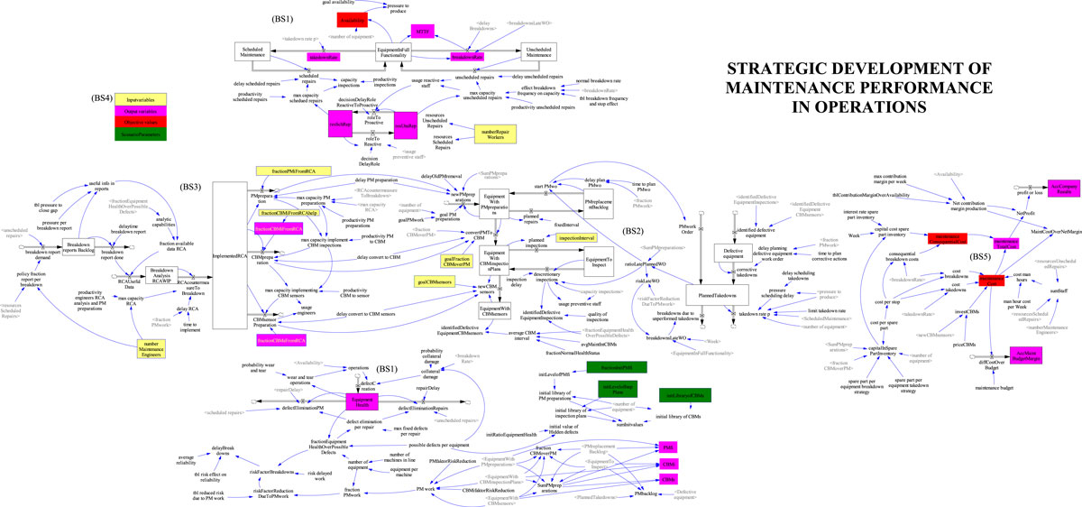
4. Overview of the conceptual SD model

This section presents a concise overview of the applied SD model in the MOO analysis. The full model includes a large feedback structure which requires much space for transcription (for the full structure and equations review, see Linnéusson et al. (2018) and the Appendix 1 where the 1:1 structure is provided together with model equations from the Vensim model). Managing maintenance in the economic short-termism framework is challenging. Therefore, the purpose of the model is to support investigating the causal relationships between strategic initiatives and performance results as well as enable analyses that take into consideration the time delays between different actions, which Tsang (2000) has sought from future researchers. The model boundary selection (BS) includes, according to Linnéusson et al. (2018), aspects such as:

BS1.	Equipment health and its interaction with the operating load of production.
BS2.	Enable the analysis of different applied maintenance methodologies and their optional mix.
BS3.	Evaluate processes of continuous improvement of maintenance performance.
BS4.	Direct and indirect maintenance resources working reactively or proactively.
BS5.	Estimate the total costs for the complete analysis, such as reactive and proactive trade-offs.

The SD model overview in Figure 1 concisely describes the maintenance performance model, including the boundary selections (BS) above, to clearly point out their relevance to the model with their subsequent descriptions below. Each box in the figure has structures of stocks and flows of a different size, which are the building blocks in SD modelling (accessible in the Appendix 1).

Figure 1. Overview of the maintenance performance SD model.

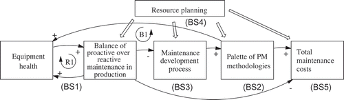
BS1 includes the equipment health (EH) structure and its interaction with the maintenance performance in production (MPP), which at any moment in time has a certain balance of proactive over reactive maintenance in production (MPP). The EH is represented by a stock of accumulated defects, whose flows are governed by the result of the MPP, where defects are reduced by planned or unplanned repairs and defects are generated by collateral damage from the breakdown rate in production and the continuous operation load. There is a reinforcing feedback (R1) in these flows of hidden defects, where the poorer EH causes more reactive breakdowns and thus more collateral damage, making EH even poorer. Reversely, better EH leads to less need for reactive maintenance, however, it depends on the support of BS2. Availability (A _T) is the result of the MPP, where reactive work and proactive work both aim at retaining equipment at full functionality; however, they do so through different feedback structures in the model, thus, with different effects on total costs (C _T).

BS2 supports the improvement of EH by the wise application of preventive maintenance methodologies (PMM). Therefore, with an improved palette of PMM, it supports the efficiency of defect identification where, for instance, condition-based monitoring using sensors (CBM_s), through its online monitoring, is perhaps more efficient than PM using fixed interval (PM_fi). The applied palette of PM methodologies also includes CBM using discretionary inspections by maintenance staff at the interval (CBM_i). These three methodologies are different in character. They have different planning triggers for work orders and different capabilities for detecting anomalies. For example, PM_fi has a fixed average delay for initiating work orders and a fixed number of parts to repair. CBM_i, on the other hand, is initiated at the interval and each inspection is performed if the staff are available. This results in a certain number of parts to repair, depending on the level of EH. However, the optimal mix is not evident, as the results of the MOO analysis in this study indicate.

BS3 indicates that the palette of PM methodologies can be improved, while the maintenance development process is a delay structure that transforms information from breakdown reports into countermeasures based on root cause analyses (RCA) of available information. Different policies for retrieving information and the process to transform it can be formulated, for instance, whether the number of maintenance engineers (S _E) affects the flow of RCA. Its delayed output may be new PM preparations, or the development of old ones, changing the mix between PM_fi, CBM_i, and CBM_s and its total relation to all parts of the system. This means any scenario of between 0 and 100% PM work can be subject to experimentation as well as any of the varying optional mix of the methodologies.

Now the balancing loop B1 can be closed, which describes the continuous improvement generated by the need for increased capabilities to maintain EH at an acceptable level. Poorer EH leads to poorer MPP with a high rate of breakdowns (R _BD), for which repair workers document, if known, their causes. Through the analyses of engineers (S _E), this eventually results in improved PM preparations of either PM_fi, CBM_i, or CBM_s. It also leads to more efficient PM work and has a greater impact on the EH through the more proactive balance of preventive repairs in production.

BS4 nonetheless regards that the dedicated resource planning, to a large extent, decides upon the effective result through the above-mentioned feedback mechanisms. Three types of staff resources are included, engineers (S _E) and repair workers (S _R) working proactively or reactively. S _E is dedicated to their tasks throughout the simulation period, while the S _R move between their working pools according to the workload created from the R _BD. If R _BD persists, S _R cannot work proactively, however, if the R _BD increases, proactive S _R staff will help and support the acute need.

BS5 sums up the total maintenance costs (C _T) as a consequence of the palette of PMM, including maintenance costs (C _M) of staff and spare parts, investment costs in CBM_s and consequential maintenance costs (C _Q) from breakdowns and tied up capital in the spare parts inventory. This structure also contains the accumulation of the maintenance budget accomplishment and the accumulated profits throughout the simulation period – the accumulated economic result (E _R). As the overview in Figure 1 illustrates, there is no feedback from the C _T back to the other structure, hence, the measures in BS5 do not impact any of the endogenously created dynamics, which could be the case for another system boundary.

5. Validation SD model

Validation of the SD model has considered the normal techniques in SD, applying the formal validation tests according to Barlas (1996):

• Direct structure tests have been followed, which constitute purely qualitative comparisons with the literature and knowledge about the real-world system provided by the study of two large maintenance organisations.

• Structure-oriented behaviour tests have been followed to a large extent. Such tests utilise the quantitative simulation to evaluate the capability of the structures to represent the expected feedback behaviours, by the application of extreme condition tests, behaviour sensitivity tests, and boundary adequacy tests.

• Behaviour pattern tests do not provide added value to validate the model structure (Barlas, 1996), but validates the generated behaviour. However, the conceptual model does not include parameter face values which need an application case where direct input data is taken from the real-world system.

The tests have resulted, to some extent, in justifying the overall model behaviour. They have also included the testing of assumptions, with the help of industrial maintenance experts. Furthermore, the application of MOO has resulted in strengthening the structure-oriented behaviour test, by exploring errors in the model, as mentioned previously and described schematically in Figure 3. Consequently, model equations have been improved, adding some parameters and new structures, compared to the conceptual SD model presented in the study by Linnéusson et al. (2018).

6. Model formulation and policy experimentation: Applying MOO with SD

The simulation principle for evaluating SD models using MOO follows the general SBO process illustrated in Figure 2, where the “Simulation Model” is regarded as a “Black Box” for the optimisation engine. The SD model was built in Vensim DSS and the MOO simulation model in modeFrontier. The integration of MOO and SD has followed the MOO + SD methodology developed by Aslam (2013), which in detail describes the steps of decision space sampling, global objective space search, and local objective space refinement. This leads to the presentation of optimal solutions which are part of step 4 in the general procedure for an MOO + SD analysis, illustrated in Figure 3. The MOO simulation model utilises the NSGA-II algorithm and the evaluation process activates and executes multiple runs of the SD model. In the literature, Fast Elitist Non-Dominated Sorting Genetic Algorithm (NSGA-II), developed by Deb, Pratap, Agarwal, and Meyarivan (2002), is probably the best-known population-based metaheuristic algorithm for giving very good approximations of the Pareto front; according to Zhou et al. (2011), a majority of research and application areas applying multi-objective evolutionary algorithms are sharing more or less the same framework as that of NSGA-II. Three major features have rendered the outstanding performance of NSGA-II which make it to be chosen for this work: (1) an elitism principle, based on a λ + μ elitism selection procedure; (2) the calculation of crowding distance value for an explicit and efficient diversity preserving mechanism that eliminates an extra niching parameter used in other MOO algorithms; (3) non-dominated solutions is emphasised by equipping with a fast non-dominated sorting approach that has a complexity of O(mN²), instead of O(mN³) like Multi-Objective Genetic Algorithm (Babbar, Lakshmikantha, & Goldberg, 2003).

Figure 2. The general SBO process, adapted from (Aslam, 2013).

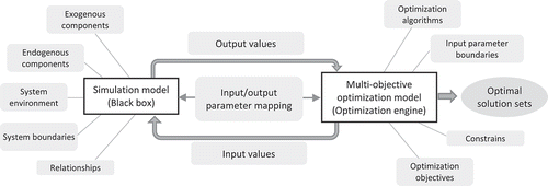
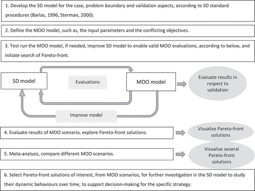
Figure 3. The general procedure for an MOO + SD analysis.

Furthermore, the presented optimisation scenarios in this study are the result of applying an initial DOE (design of experiments) with 50 randomised values on the inputs, presented in Table 2, run for 100 generations, totalling 5000 evaluations. The generated initial population of Pareto-front solutions was then used as “a trained DOE”, run for the number of generations that resulted in a final solution set of at least 50,000 evaluations.

Table 2. Input parameter data for the MOO.

Input parameter in SD model	Notation	Range	Step	Note
numberRepairWorkers	S R	4–50	1	Total work pool of repair staff
numberMaintenanceEngineers	S E	0–30	1	Staff dedicated to develop new PM work
fractionPMiFromRCA	F PM	0–1	0.05	These two parameters control the distribution between PMfi, CBMi, and CBMs
fractionCBMiFromRCAhelp	F CBM	0–1	0.05
goalFractionCBMoverPM	PMFCBM	0–1	0.05	Goal for CBMi + CBMs over all PM work
inspectionInterval	I I	4–52	2	Interval for inspections for CBMi
goalCBMsensors	PMCBMs	0–500	25	Goal for CBMs

The procedure for the MOO + SD analysis can generally be described according to Figure 3. Step 1 is the ordinary modelling procedure for an SD model. Step 2 includes setting up the optimisation model in the optimisation engine, based on the selected conflicting objectives in the SD model and output parameters of interest. Step 3 includes evaluating the initial results, which most certainly will require further improvements of the validity of the SD model since the MOO evaluations expose any inability of the SD model to generate a valid answer. When step 3 reveals valid answers, step 4 can start with the aim to generate analysable results, such as the subsequent scatter plots and parallel coordinates in the results and analysis section. Step 5 represents the comparison of several scenarios, as performed in this study. Step 6 represents post-analyses of solutions of interest, where a Pareto-front solution can be analysed in the SD software more deeply, in order to investigate the feedback dynamics of its performance; however, this is not explored further in this paper.

7. Application of MOO to the maintenance performance model

The MOO scenarios represent companies at different states of developed maintenance performance.

Thus, each scenario seeks to evaluate the same input parameters, and the same ranges of these, according to Table 2. The input parameters are selected in the SD model on the basis of their expected effects that can lead to the attainment of a proactive behaviour in maintenance. The aim of each optimisation scenario is to identify the most beneficial development towards a future state in the SD model, which uses a time horizon of 10 years. This is applied using the optimisation objectives of maximising availability, max (A _T), minimising maintenance costs, min (C _M), and minimising maintenance consequential costs, min (C _Q).

The scenarios represent three different initial conditions, to which some companies can relate, which differ accordingly:

• Scenario S1 represents companies applying a Run-To-Failure (RTF) strategy, using PM_fi on 5% of the equipment, including, for example, lubrication and the minimal activities due to warranty requirements.

• Scenario S2 represents companies applying a somewhat mediocre PM performance, with an RTF strategy for 50% of the equipment and 50% using PM_fi.

• Scenario S3 represents companies with highly developed and well-performing PM work, with 75% PM_fi, 20% of CBM_i, and 5% CBM_s.

8. Results and analysis

To pursue the analysis, firstly, the scatter plots of the optimised trade-off behaviour between the three conflicting objectives are analysed. Secondly, the parallel coordinate heat maps (PCHM), covering a set of selected parameters, are analysed to identify their patterns of dependence.

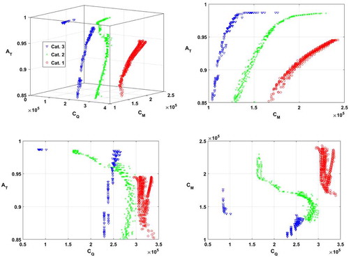
8.1. Meta-analysis of MOO scenarios using scatter plots

The results, in Figure 4, include four perspectives of the same sets of solutions, where scenario S1 is the category 1 circular dots, scenario S2 is the category 2 x-shaped dots and scenario S3 is the category 3 triangle-shaped dots. The left-hand side upper plot has a 3D perspective, including all three optimisation objectives, which the other 2D plots are oriented toward. All Pareto-front solutions for scenarios S1, S2, and S3 are significantly apart. The right-hand side upper plot reveals a linear dependency between availability (A _T) and maintenance cost (C _M), where the consequence of increased equipment utilisation leads to a higher C _M. Both S2 and S3 exhibit a knee region, characterised by the fact that a small increase in A _T has induced a considerably higher C _M. S1 solutions do not have such a “knee” region and reach about A _T = 0.95. In the left-hand side lower plot, especially S2 and S3 solutions reveal a non-linear characteristic, where increased A _T leads to decreased maintenance consequential costs (C _Q), although initially, they follow a near linear dependency on higher C _Q as A _T increases. It means that the high-performing solutions probably achieve the availability through a proactive behaviour in the SD model since attaining high availability through a reactive behaviour generates substantial consequential breakdown costs and a larger spare parts inventory. With this in mind, S1 solutions in the C _Q A _T plot on the left-hand side exhibit a rather linear shape. Interestingly, at about A _T = 0.95, there are S2 solutions that perform lower C _Q than the S3 solutions. Nonetheless, the top-performing solutions in S3 outperform all others, with respect to C _Q. The right-hand side lower plot reveals the characteristic relation between the performance of C _M and the C _Q. Studying S1 in that plot reveals that there is little benefit from increasing C _M. However, in S2 and S3, the relation between C _M and C _Q has shown some dramatic changes. In S2, at higher C _M than about 150,000, a further increase in availability causes a steady decrease in C _Q until at about 200,000, where no further benefit is shown. S3 solutions behave similarly, but much more rapidly, with a large gap between Pareto-front solutions on the scale of C _Q.

Figure 4. Scatter plots for the three scenarios.

Hence, the Pareto-front results in Figure 4 clearly reveal the trade-off between the three optimising objectives: max (A _T), min (C _M), and min (C _Q). Firstly, they can be considered very different in character, as comparing the patterns of solutions for each scenario reveals. Secondly, they exhibit a perception of the possible path to development within each scenario, as indicated in the characteristics of system inertia, depending on the scenario and selected strategies.

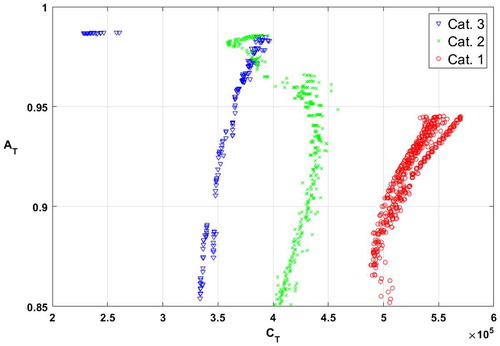
The x-axis of the 2D scatter plot in Figure 5 represents the summation of the two cost objectives: C _T = C _M + C _Q. In S1, C _T increases with higher A _T until 0.94, but when A _T approaches 0.95, C _T are lower for some solutions. S2 solutions clearly produce a non-linear behaviour, where higher A _T up to about 0.92 is linear. From that area, each increase in A _T leads to a considerable decrease in C _T, until a point where a further increase is very expensive. Studying the PCHM in Figure 7 reveals that these solutions are characterised by having fewer breakdowns (R _BD) and more takedowns (R _TD). S3 solutions exhibit a behaviour which at first shows that there is a small increase in C _T as A _T increases, then above 0.98, there are radically better solutions with a gap in between; in the PCHM of Figure 8, this appears as two clusters of solutions.

Figure 5. 2D scatter plot for the three scenarios.

8.2. Meta-analysis of MOO scenarios using PCHM

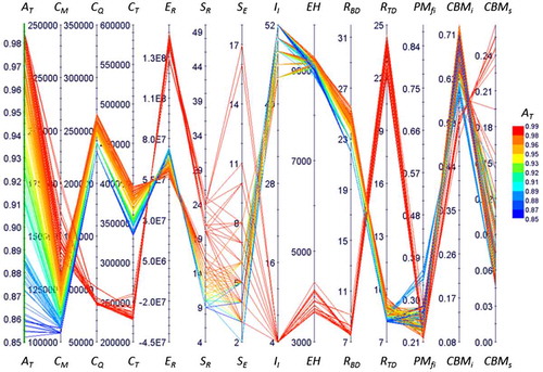
The parallel coordinate heat maps (PCHM) of the scenarios enable a meta-analysis of the results. Each line in the PCHM represents one set of Pareto-front solutions, which enables analysing the dependency between parameter results and distinguishes the characteristics of the solutions from each other. The first four axes in Figures 6–8 are the parameters presented in the above scatter plots: A _T, C _M, C _Q, and C _T, respectively. Thus, the same information is presented in the PCHM-format. For instance, studying the 3D scatter plot 3 in Figure 5 reveals that some solutions in S2 are better than in S3; identify these on the 3rd axis and follow the lines to the breakdown rate (R _BD) and the takedown rate (R _TD) axis, where the best S2 solutions have more planned maintenance activities compared to the inferior cluster of solutions in S3. In addition, looking at the accumulated economic results (E _R) on the 5th axis in the PCHMs shows that all S1 solutions have a negative result, thus, they may not be worth aiming for with respect to profit. However, S2 and S3 have solutions with positive E _R and in addition S3 has some very high performing solutions. The next two parameters are the staff of repair workers (S _R) and maintenance engineers (S _E), where S1 solutions require high levels of S _R and S _E. S2 solutions are represented on a large range of S _R and more S _E than S1. Furthermore, S3 manages with fewer S _R and has even more S _E. The next parameter, the inspection interval (I _I), shows that all solutions for S1 use a short interval, solutions for S2 are represented on the complete range and S3 solutions are either concentrated on short intervals or long intervals. The performance of S1 solutions, on the EH axis of the equipment health parameter, is on a rather narrow range and on quite a high level of hidden defects, which is its units. For S2, there is a large range spanning from a high to a low level of hidden defects and, for S3, there are two clear clusters of solutions at both ends of the S2 range on EH. The next two parameters indicate the result of unplanned and planned maintenance interventions, where S1 solutions have a high breakdown rate (R _BD), with a narrow range and few takedowns (R _TD). A similar pattern is found for the poor performing solutions in S2, while the better performing cluster has an opposite relation. For S3, there are clearly two separate clusters that either perform very well, or similar, on the poor performing solutions in S2. The last three parameters in the PCHMs provide information on the distribution between the different maintenance methodologies, namely, PM_fi, CBM_i, and CBM_s respectively. By comparing S1, S2, and S3, three different patterns are obvious. S1 solutions generally use the most PM_fi, then CBM_i and thereafter CBM_s. In S2 solutions, three patterns can be distinguished; first, solutions using more than 50% PM_fi, which also use about 10% CBM_i and most CBM_s. The second clear pattern which also represents solutions that perform best on A _T contains solutions that use less than 50% PM_fi, almost 50% CBM_i or more, as well as a low level of CBM_s. The third pattern can be distinguished in the middle of the PM_fi axis. These solutions use approximately 50% PM_fi and about 40% CBM_i, as well as CBM_s on an almost 10% range. S3 solutions, whose results on previous parameters have been very clearly divided into two patterns, are not so different here, where solutions are rather concentrated for both PM_fi and CBM_i. However, for S3 solutions on the CBM_s axis, some of the best-performing solutions on availability differ with a higher level of CBM_s, but they also exist on the lower range down to 5% CBM_s.

Figure 6. PCHM for scenario 1.

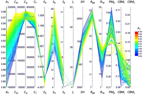
Figure 7. PCHM for scenario 2.

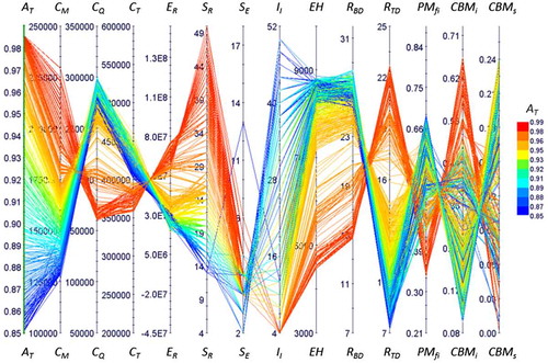
Figure 8. PCHM for scenario 3.

8.3. Summary MOO meta-analysis

Generally, the meta-analysis indicates that S1 solutions are more homogenous, whereas S2 and S3 have at least two clusters of behaviour. Studying all the top performing solutions in all the graphs on the axes of different parameters; S _E is a common denominator, indicating the significance of engineers to the development process of more proactive maintenance. Another aspect is the considerable diversity of maintenance methodologies (PM_fi, CBM_i, CBM_s) for the solutions. Each scenario exhibits its own separate pattern, indicating the importance of considering the initial condition when choosing the strategy to apply in order to achieve the most successful PM behaviour in production.

S1 reveals that a journey towards a proactive maintenance behaviour, with the initial condition of using an RTF strategy, may not provide enough profit, see E _R. It means that the profit per production volume needs to be higher for a company in S1 than for a company in S2 and S3. It indicates that companies with inadequately developed and poor-performing PM work may be better off by continuing with reactive maintenance. This result could clarify the statement, according to Sharma, Kumar, and Kumar (2005), that using a breakdown maintenance strategy is a feasible approach in situations with high customer demands and large profit margins. However, as a matter of fact, the MOO analysis reveals that the potential to be proactive is still prominent in such a system that S1 represents, see Figure 6, where solutions with a higher R _TD perform best in A _T and C _Q. Hence, if profit margins are large enough, the negative spiral of reactiveness can be broken if such a strategy is pursued.

S2 solutions perform on a large range of C _M, see Figure 7, where high-cost solutions clearly result in the overall best PM performance, with lowest C _Q. S2 represents a company with an initial, mediocre level of maintenance performance and, in order to attain the higher region of A _T, the analysis clearly indicates the need for S _R. Comparing the high A _T solutions to the low A _T solutions, which have low C _M, indicates they definitively suffer from an overbalance toward R _BD instead of planned R _TD.

S3 reveals that distinctly better performing future states are attainable, see Figure 8. S3 stands out from S1 and S2 using considerably more engineers (S _E), which indicates that the initial conditions may be highly significant for whether the capabilities of S _E can be put into effect or whether doing so is just a waste of resources. Nevertheless, S3 clearly indicates that, when the inertia in the maintenance and production system overcomes the tipping point into a proactive maintenance behaviour, it excels in performance. The characteristics, seen in S3, that generate such proactive maintenance behaviour is keeping the hidden defects in the parameter EH at a low level. The strategy applied in the top performing solution sets is attained by a high R _TD based on identified defects mainly through CBM_i, followed by a rather high level of CBM_s and PM_fi on the lowest share. Nevertheless, such a strategy must also be supported by accurate levels of S _R and S _E, to enable the corresponding development of precision activities, based on facts about the equipment and its failure behaviours.

9. Conclusions and future work

This paper presents a study which applies simulation-based optimisation (SBO), using multi-objective optimisation (MOO) on a conceptual, system dynamics (SD) maintenance performance model. This integration provides a method for the thorough analysis of the trade-offs between conflicting objectives, such as maximise availability, minimise maintenance costs, and minimise maintenance consequential costs.

The study compares three MOO scenarios with different initial conditions of preventive maintenance, which result in a certain performance and behaviour in the model. The results strongly indicate the nonlinearity between maintenance costs and maintenance consequential costs, especially at the higher levels of developed, preventive maintenance performance. The results clearly reveal that the different initial conditions require different strategies for the development of maintenance performance. The use of parallel coordinate heat maps (PCHM) enables the analysis to identify why the scenarios perform differently and explains the characterisation of solutions on the efficient frontiers. The results make explicit the implication of path dependency, regarding the development rate of maintenance performance for the different scenarios. This depends both on the current state and on how policies are formulated on the journey towards an improved future state. Consequently, using MOO with an SD model, as proposed in this paper, exhibits a very rich quantitative analysis to support the decision-making on a possible, future action strategy for the system under study.

The results and insights gained from the conceptual model, described in this paper, cannot be generalised for all practical maintenance situations which require the development of more detailed models of production facilities and complex cost models. However, it is believed that the SBO framework, using MOO analysis on SD models, is readily applicable to more complex, detailed models for more complicated analyses of maintenance performance. In other words, it can be said that the limitation of the paper is posed by the detailed level of the SD models, but not the SBO framework.

Additionally, with respect to validation, an MOO analysis allows an extreme and thorough evaluation of possible simulation runs of the applied SD model, which clearly reveals its capacity to calculate reasonable results. For this study, the applied model had to be improved to show any meaningful results, hence applying MOO to explore a conceptual SD model has contributed to strengthening its use. As such, this can be considered a positive side effect in the process of achieving increased validation for its applicability.

In this regard, the application of MOO to explore an SD model can be considered a valuable contribution to support the formulation of a maintenance strategy, compared to experimenting in an SD model without knowing whether the experiments are close or far from the optimal trade-offs. Nonetheless, in order to connect strategy and operational execution, future work will investigate the combination of this proposed framework with discrete event simulation (DES) to prioritise maintenance activities at the operational level. Combining SD with DES is an evolving research topic, and has been promoted, due to its ability to dramatically increase the size of the scenario landscape, as well as utilising the strengths of the two approaches, such as feedback into DES and details into SD (Sasdad et al., 2014). In other words, future work will explore a mixed method approach that considers both the planning of the short-term, maintenance tasks and the improvement of long-term strategic planning as in this paper. By integrating the DES and SD modelling approaches using MOO, it will be possible to explore an integrated SBO framework with the potential to address industrial maintenance problems that stretch the interface between strategic and operational levels. Overall speaking, such a framework can allow maintenance to be in charge of its own optimal planning, instead of reacting and following other requirements set by production or poorly defined priorities of activities.

Disclosure statement

No potential conflict of interest was reported by the authors.

Funding

This work was partially financed by the Knowledge Foundation (KKS), Sweden, through the IPSI Research School.

Acknowledgements

The authors gratefully acknowledge their provision of the research funding and the support of the industrial partners Volvo Car Corporation and Volvo Group Trucks Operations.

Appendix 1.

Model structure

Model equations from Vensim

Table

Variable name	Expression	Unit
AccCompanyResults	INTEG (profit or loss,0)	$
AccMaintBudgetMargin	INTEG (diffCostOverBudget, 0)	$
analytic capabilities	1-fractionEquipmentHealthOverPossibleDefects	Dmnl
Availability	EquipmentInFullFunctionality/number of equipment	Dmnl
average CBM interval	avgMaintIntCBMs/(fractionEquipmentHealthOverPossibleDefects/fractionNormalHealthStatus)	Week
average reliability	52	Week
avgMaintIntCBMs	104	weeks
breakdown report demand	unscheduled repairs*policy fraction report per breakdown	info/Week
breakdown report done	Breakdown reports Backlog/delaytime breakdown report	info/Week
Breakdown reports Backlog	INTEG ( breakdown report demand-breakdown report done, 0)	info
BreakdownAnalysisRCAWIP	INTEG (RCAUsefulData-RCAcountermeasureToBreakdown, 0)	info
breakdownRate	EquipmentInFullFunctionality/delayBreakdowns + breakdownsLateWO	equipment/Week
breakdowns due to unperformed takedowns	breakdownsLateWO	equipment/Week
breakdownsLateWO	riskLateWO*EquipmentInFullFunctionality/Week	equipment/Week
capacity inspections	MAX(max capacity scheduled repairs – scheduled repairs , 0) * productivity inspections	equipment/Week
capital cost spare part inventory	interest rate spare part inventory/Week * capitalInSparePartInventory	$/Week
capitalInSparePartInventory	(spare part per equipment breakdown strategy*(number of equipment-SumPM preparations) + spare part per equipment takedown strategy*((1-fractionCBMoverPM) + 0.5*fractionCBMoverPM) * SumPMpreparations) * cost per spare part	$
CBMi	(EquipmentToInspect + EquipmentWithCBMinspectionPlans)/SumPMpreparations	Dmnl
CBMifaktorRiskReduction	0.8	Dmnl
CBMpreparation	MIN(ImplementedRCA*fractionCBMiFromRCA/delay convert to CBM , max capacity implement CBM inspections)	info/Week
CBMs	EquipmentWithCBMsensors/SumPMpreparations	Dmnl
CBMsensorPreparation	MIN(ImplementedRCA*fractionCBMsFromRCA/delay convert to CBM sensors , max capacity implementing CBM sensors)	info/Week
collateral damage	breakdownRate*probability collateral damage*possible defects per equipment	defects/Week
consequential breakdown costs	4*cost per stop * breakdownRate	$/Week
convertPMToCBM	MIN(MAX(0,(goalFractionCBMoverPM*EquipmentWithPMpreparations-fractionCBMoverPM* EquipmentWithPMpreparations)/delay convert to CBM), CBMpreparation*PM preparation release)	equipment/Week
corrective takedowns	Defective equipment/delay planning defective equipment work order	equipment/Week
cost breakdowns	cost per stop*breakdownRate	$/Week
cost man hours	man hour cost per Week*sumStaff	$/Week
cost per spare part	2000	$/equipment
cost per stop	1.25*cost per spare part	$/equipment
cost takedowns	cost per stop*takedownRate	$/Week
decisionDelayRole	12	weeks
decisionDelayRoleReactiveTo Proactive	4	weeks
defect elimination per repair	MAX(max fixed defects per repair* fractionEquipmentHealthOverPossibleDefects , 1)	defects/equipment
defectCreation	operations + collateral damage	defects/Week
defectEliminationPM	MIN(scheduled repairs*defect elimination per repair, EquipmentHealth/repairDelay)	defects/Week
defectEliminationRepairs	MIN(unscheduled repairs*defect elimination per repair, EquipmentHealth/repairDelay)	defects/Week
Defective equipment	INTEG (identified defective equipment-corrective takedowns, 1)	equipment
delay convert to CBM	26	Week
delay convert to CBM sensors	52	Week
delay plan PMwo	time to plan PMwo/(MIN(fractionPMwork , 0.5)*2)	Week
delay planning defective equipment work order	time to plan corrective actions/(MIN(fractionPMwork , 0.5)*2	Week
delay PM preparation	13	Week
delay RCA	time to implement/(MIN(fractionPMwork , 0.8)*2)	weeks
delay scheduled repairs	0.05	Week
delay scheduling takedowns	1	Week
delay unscheduled repairs	0.1	Week
delayBreakdowns	tbl risk effect on reliability(riskFactorBreakdowns) * average reliability	Week
delayOldPMremoval	26	weeks
delaytime breakdown report	1	weeks
diffCostOverBudget	maintenance budget –maintenanceCost	$/Week
discretionary inspections	IF THEN ELSE(ratioLatePlannedWO> = 0.1, 0, IF THEN ELSE(capacity inspections> = 2* (EquipmentToInspect/inspection delay), MIN(2*EquipmentToInspect/inspection delay, capacity inspections), MIN(EquipmentToInspect/inspection delay, capacity inspections)))	equipment/Week
effect breakdown frequency on capacity	tbl breakdown frequency and stop effect(breakdownRate/normal breakdown rate)	Dmnl
equipment per machine	25	equipment/machine
EquipmentHealth	INTEG (defectCreation-defectEliminationPM-defectEliminationRepairs, initial value of Hidden defects*number of equipment)	defects
EquipmentInFullFunctionality	INTEG (scheduled repairs + unscheduled repairs-breakdownRate-takedownRate, 0.622*number of equipment)	equipment
EquipmentToInspect	INTEG (planned inspections-descretionary inspections, 0)	equipment
EquipmentWithCBMinspectionPlans	INTEG (convertPMToCBM-newCBMsensors-planned inspections + descretionary inspections, initial library of inspection plans)	equipment
EquipmentWithCBMsensors	INTEG (newCBMsensors, initial library of CBMs)	equipment
EquipmentWithPMpreparations	INTEG (newPMpreparations + start PMwo-convertPMToCBM-planned repairs, initial library of PM preparations)	equipment
FINAL TIME	520	Week
fixedInterval	52	Week
fraction available data RCA	useful info in reports * analytic capabilities	Dmnl
fractionCBMiFromRCA	(1-fractionPMiFromRCA)*fractionCBMiFromRCAhelp	Dmnl
fractionCBMiFromRCAhelp	0.45	Dmnl
fractionCBMoverPM	(EquipmentToInspect + EquipmentWithCBMinspectionPlans + EquipmentWithCBM sensors)/(PMreplacementBacklog + EquipmentToInspect + EquipmentWithCBM inspectionPlans + EquipmentWithCBMsensors + EquipmentWithPMpreparations)	Dmnl
fractionCBMsFromRCA	1-fractionCBMiFromRCA-fractionPMiFromRCA	Dmnl
fractionEquipmentHealthOverPossibleDefects	EquipmentHealth/(number of equipment*possible defects per equipment)	Dmnl
fractionInitPMfi	0.5	Dmnl
fractionNormalHealthStatus	0.7	Dmnl
fractionPMiFromRCA	0.5	Dmnl
fractionPMwork	PM work/number of equipment	Dmnl
goal availability	0.9	Dmnl
goal PM preparations	number of equipment*goalPMwork	equipment
goalCBMsensors	25	equipment
goalFractionCBMoverPM	0.3	Dmnl
goalPMwork	1	Dmnl
identified defective equipment	identifiedDefectiveEquipmentInspections + identifiedDefectiveEquipmentCBMsensors	equipment/Week
identifiedDefectiveEquipment CBMsensors	EquipmentWithCBMsensors/average CBM interval	equipment/Week
identifiedDefectiveEquipment Inspections	discretionary inspections * fractionEquipmentHealthOverPossibleDefects * quality of inspections	equipment/Week
ImplementedRCA	INTEG (RCAcountermeasureToBreakdown-CBMpreparation-CBMsensorPreparation-PMpreparation,1)	info
initial library of CBMs	initLibraryofCBMs*number of equipment	equipment
initial library of inspection plans	initLevelofInspPlans * number of equipment	equipment
initial library of PM preparations	initLevelofPMfi*number of equipment	equipment
INITIAL TIME	0	Week
initial value of Hidden defects	initRatioEquipmentHealth*possible defects per equipment	defects/equipment
initLevelofInspPlans	0.001	Dmnl
initLevelofPMfi	fractionInitPMfi	Dmnl
initLibraryofCBMs	0.001	Dmnl
initRatioEquipmentHealth	0.7737	Dmnl
inspection delay	2	Week
inspectionInterval	4	Week
inspectionInterval	4	Week
interest rate spare part inventory	0.4	Dmnl
investCBMs	newCBMsensors*priceCBMs	$/Week
limit takedown rate	0.05	Dmnl
MaintCostOverNetMargin	maintenanceCost/Net contribution margin production	Dmnl
maintenance budget	100,000	$/Week
maintenanceConsequentialCost	consequential breakdown costs + capital cost spare part inventory	$/Week
maintenanceCost	cost man hours + cost breakdowns + cost takedowns + investCBMs	$/Week
maintenanceTotalCost	maintenanceConsequentialCost + maintenanceCost	$/Week
man hour cost per Week	2400	$/(Person*Week)
max capacity implement CBM inspections	(max capacity PM preparations-PMpreparation) * productivity PM to CBM	info/Week
max capacity implementing CBM sensors	(max capacity implement CBM inspections-CBMpreparation) * productivity CBM to sensor	info/Week
max capacity PM preparations	(max capacity RCA – RCAcountermeasureToBreakdown)*productivity PM preparations	info/Week
max capacity RCA	numberMaintenanceEngineers*productivity engineers RCA analysis and PM preparations	info/Week
max capacity schedued repairs	resSchRep*productivity scheduled repairs	equipment/Week
max capacity unscheduled repairs	resUnsRep*productivity unscheduled repairs/effect breakdown frequency on capacity	equipment/Week
max contribution margin per week	600,000	$/Week
max fixed defects per repair	8	defects/equipment
MTTF	EquipmentInFullFunctionality/breakdownRate	Week
Net contribution margin production	Availability * max contribution margin per week * tblContributionMarginOverAvailability(Availability)	$/Week
NetProfit	Net contribution margin production – maintenanceTotalCost	$/Week
newCBMsensors	IF THEN ELSE(goalCBMsensors > EquipmentWithCBMsensors, MIN( CBMsensor Preparation*PM preparation release, MIN((goalCBMsensors-EquipmentWithCBM sensors)/delay convert to CBM sensors, MAX(0 , EquipmentWithCBMinspectionPlans/delay convert to CBM sensors))) , 0)	equipment/Week
newPMpreparations	MIN((goal PM preparations-SumPMpreparations)/delay PM preparation, PMpreparation*PM preparation release) – IF THEN ELSE(goal PM preparations < SumPMpreparations, EquipmentWithPMpreparations/delayOldPMremoval, 0)	equipment/Week
normal breakdown rate	18	equipment/Week
number of equipment	number of machines in line*equipment per machine	equipment
number of machines in line	20	machines
numberMaintenanceEngineers	3	people
numberRepairMen	10	people
operations	Availability * wear and tear operations	defects/Week
planned inspections	EquipmentWithCBMinspectionPlans/inspectionInterval	equipment/Week
planned repairs	EquipmentWithPMpreparations/fixedInterval	equipment/Week
PlannedTakedowns	INTEG (corrective takedowns + PMworkOrder-breakdowns due to unperformed takedowns-takedown rate p – breakdowns due to unperformed takedowns, 4)	equipment
PM preparation release	1	equipment/info
PM work	EquipmentWithCBMinspectionPlans*CBMifaktorRiskReduction + EquipmentWithCBM sensors + EquipmentWithPMpreparations*PMfaktorRiskReduction	equipment
PMbacklog	PMreplacementBacklog + EquipmentToInspect + Defective equipment + PlannedTakedowns	equipment
PMfaktorRiskReduction	0.5	Dmnl
PMfi	(EquipmentWithPMpreparations + PMreplacementBacklog)/SumPMpreparations	Dmnl
PMpreparation	MIN(ImplementedRCA*fractionPMiFromRCA/delay PM preparation , max capacity PM preparations)	info/Week
PMreplacementBacklog	INTEG (planned repairs-start PMwo, 0)	equipment
PMtotal	SumPMpreparations/number of equipment	Dmnl
PMworkOrder	start PMwo	equipment/Week
policy fraction report per breakdown	IF THEN ELSE(numberMaintenanceEngineers > 0 :AND: resourcesScheduledRepairs > 0, 1, 0)	info/equipment
possible defects per equipment	20	defects/equipment
pressure per breakdown report	1	1/info
pressure scheduling delay	(delay scheduling takedowns*pressure to produce)	Week
pressure to produce	MIN(MAX(1, goal availability/Availability) , 4)	Dmnl
priceCBMs	10,000	$/equipment
probability collateral damage	0.25	Dmnl
probability wear and tear	0.015	1/Week
productivity CBM to sensor	0.5	Dmnl
productivity engineers RCA analysis and PM preparations	10	info/(Week*people)
productivity inspections	2*0.8	Dmnl
productivity PM preparations	0.5	Dmnl
productivity PM to CBM	0.1	Dmnl
productivity scheduled repairs	36 * 0.2	equipment/(Week*people)
productivity unscheduled repairs	9 * 0.5	equipment/(Week*people)
profit or loss	NetProfit	$/Week
quality of inspections	1	Dmnl
ratioLatePlannedWO	PlannedTakedowns/SumPMpreparations	Dmnl
RCAcountermeasureToBreakdown	MIN(BreakdownAnalysisRCAWIP/delay RCA , max capacity RCA)	info/Week
RCAUsefulData	breakdown report done*fraction available data RCA	info/Week
repairDelay	1	Week
resourcesScheduledRepairs	0.2*numberRepairMen	people
resourcesUnscheduledRepairs	0.8*numberRepairMen	people
resSchRep	INTEG (roleToProactive-roleToReactive, resourcesScheduledRepairs)	people
resUnsRep	INTEG (roleToReactive-roleToProactive, resourcesUnscheduledRepairs)	people
risk delayed work	2	Dmnl
riskFactorBreakdowns	fractionEquipmentHealthOverPossibleDefects * (risk delayed work/riskFactorReductionDueToPMwork)	Dmnl
riskFactorReductionDueToPMwork	tbl reduced risk due to PM work(fractionPMwork)	Dmnl
riskLateWO	ratioLatePlannedWO/riskFactorReductionDueToPMwork	Dmnl
roleToProactive	IF THEN ELSE(resUnsRep < 1, 0, IF THEN ELSE(resUnsRep > 4:AND:usage reactive staff < 0.75, 1, IF THEN ELSE(resUnsRep < 4:AND:usage reactive staff < 0.5, 1, 0)))/decisionDelayRoleReactiveToProactive	people/Week
roleToReactive	IF THEN ELSE(resSchRep < 1, 0, IF THEN ELSE(resSchRep > 4:AND:usage preventive staff < 0.75, 1, IF THEN ELSE(resSchRep > 2:AND:usage preventive staff < 0.5, 1, 0)))/decisionDelayRole	people/Week
SAVEPER	13	Week [0,?]
scheduled repairs	MIN(ScheduledMaintenance/delay scheduled repairs , max capacity schedued repairs)	equipment/Week
ScheduledMaintenance	INTEG ( takedownRate-scheduled repairs, 0)	equipment
spare part per equipment breakdown strategy	5	Dmnl
spare part per equipment takedown strategy	2	Dmnl
start PMwo	IF THEN ELSE(ratioLatePlannedWO>=0.1, 0, PMreplacementBacklog/delay plan PMwo)	equipment/Week
SumPMpreparations	PMreplacementBacklog + EquipmentToInspect + EquipmentWithCBMinspectionPlans + EquipmentWithCBMsensors + EquipmentWithPMpreparations	equipment
sumStaff	numberMaintenanceEngineers + resourcesScheduledRepairs + resourcesUnscheduledRepairs	people
takedown rate p	IF THEN ELSE(ScheduledMaintenance > limit takedown rate*number of equipment/pressure to produce, 0, PlannedTakedowns/pressure scheduling delay)	equipment/Week
takedownRate	takedown rate p	equipment/Week
tbl breakdown frequency and stop effect	([(0,0)–(4,9)],(0,1),(1,1),(2,3),(4,9))	Dmnl
tbl pressure to close gap	([(0,0)-(100,000,1)],(0,1),(1,1),(5,0.9),(10,0.7),(20,0.5),(100,0.2),(100,000,0))	Dmnl
tbl reduced risk due to PM work	([(0,0.8)-(1,2)],(0,1),(0.3,1.05),(0.6,1.4),(0.75,1.9),(1,2))	Dmnl
tbl risk effect on reliability	([(0,0)-(2.1,4)],(0,4),(0.3,3.6),(0.38,3),(0.45,1.5),(0.5,1),(0.65,0.72), (1.05,0.36),(2.1,0.1))	Dmnl
tblContributionMarginOverAvailability	( [(0,0)-(1,1)],(0,1),(0.7,1),(1,0.85))	Dmnl
TIME STEP	0.015625	Week [0,?]
time to implement	13	Week
time to plan corrective actions	1	Week
time to plan PMwo	2	Week
unscheduled repairs	MIN(UnscheduledMaintenance/delay unscheduled repairs , max capacity unscheduled repairs)	equipment/Week
UnscheduledMaintenance	INTEG (breakdownRate-unscheduled repairs, 0.378*number of equipment)	equipment
usage engineers	IF THEN ELSE(max capacity implementing CBM sensors = 0, 1, ZIDZ( CBMsensorPreparation, max capacity implementing CBM sensors))	Dmnl
usage preventive staff	ZIDZ(descretionary inspections, capacity inspections)	Dmnl
usage reactive staff	ZIDZ(unscheduled repairs, max capacity unscheduled repairs)	Dmnl
useful info in reports	tbl pressure to close gap(Breakdown reports Backlog*pressure per breakdown report)	Dmnl
wear and tear operations	tbl probability wear and tear EqpmtAge(EqpmtAge)*probability wear and tear * MIN(EquipmentHealth, 9000)	defects/Week
Week	52	Week

References

- Alabdulkarim, A. A., Ball, P. D., & Tiwari, A. (2013). Applications of simulation in maintenance research. World Journal of Modelling and Simulation, 9(1), 14–37.
- Alrabghi, A., & Tiwari, A. (2015). State of the art in simulation-based optimisation for maintenance systems. Computers & Industrial Engineering, 82, 167–182.10.1016/j.cie.2014.12.022
- Alrabghi, A., & Tiwari, A. (2016). A novel approach for modelling complex maintenance systems using discrete event simulation. Reliability Engineering & System Safety, 154, 160–170.10.1016/j.ress.2016.06.003
- Aslam, T. (2013). Analysis of manufacturing supply chains using system dynamics and multi-objective optimization (PhD thesis). University of Skövde.
- Babbar, M., Lakshmikantha, A., & Goldberg, D. E. (2003). A modified NSGA-II to solve noisy multiobjective problems. In Proceedings of Genetic and Evolutionary Computation Conference, Chicago, USA.
- Barlas, Y. (1996). Formal aspects of model validity and validation in system dynamics. System Dynamics Review, 12(3), 183–210.10.1002/(ISSN)1099-1727
- Bertrand, J. W. M., & Fransoo, J. C. (2002). Operations management research methodologies using quantitative modeling. International Journal of Operations & Production Management, 22(2), 241–264.10.1108/01443570210414338
- de Almeida, A. T., Pires, F., Rodrigo, J., & Cavalcante, C. A. V. (2015). A review of the use of multicriteria and multi-objective models in maintenance and reliability. IMA Journal of Management Mathematics, 26(3), 249–271.10.1093/imaman/dpv010
- Deb, K. (2014). Multi-objective optimization. In E. K. Burke & G. Kendall (Eds.), Search methodologies: Introductory tutorials in optimization and decision support techniques (pp. 403–449). US: Springer.10.1007/978-1-4614-6940-7
- Deb, K., Pratap, A., Agarwal, S., & Meyarivan, T. (2002). A fast and elitist multi-objective genetic algorithm: NSGA-II. IEEE Transaction on Evolutionary Computation, 6(2), 181–197.
- Dekker, R. (1996). Applications of maintenance optimization models: A review and analysis. Reliability Engineering & System Safety, 51(3), 229–240.10.1016/0951-8320(95)00076-3
- Ding, S. H., & Kamaruddin, S. (2015). Maintenance policy optimization – literature review and directions. The International Journal of Advanced Manufacturing Technology, 76(5–8), 1263–1283.10.1007/s00170-014-6341-2
- Dudas, C., Hedenstierna, P., & Ng, A. H. C. (2011). Simulation-based innovization for manufacturing systems analysis using data mining and visual analytics. In Proceedings of 4th International Swedish Production Symposium, Lund, Sweden.
- Duggan, J. (2008). Using system dynamics and multiple objective optimization to support policy analysis for complex systems. In H. Qudrat-Ullah, J. M. Spector, & P. I. Davidsen (Eds.), Complex decision making: Theory and practice (pp. 59–81). Berlin: Springer.
- Fu, M. C. (2015). Handbook of simulation optimization. New York, NY: Springer-Verlag.10.1007/978-1-4939-1384-8
- Garg, A., & Deshmukh, S. G. (2006). Maintenance management: Literature review and directions. Journal of Quality in Maintenance Engineering, 12(3), 205–238.10.1108/13552510610685075
- Günal, M. M., & Pidd, M. (2010). Discrete event simulation for performance modelling in health care: A review of the literature. Journal of Simulation, 4(1), 42–51.10.1057/jos.2009.25
- Hedenstierna, P. (2010). Applying multi-objective optimisation to dynamic supply chain models. Conradi Research Review, 6, 19–31.
- Ilgin, M., & Tunali, S. (2007). Joint optimization of spare parts inventory and maintenance policies using genetic algorithms. The International Journal of Advanced Manufacturing Technology, 34(5–6), 594–604.10.1007/s00170-006-0618-z
- Keating, E. K., Oliva, R., Repenning, N. P., Rockart, S., & Sterman, J. (1999). Overcoming the improvement paradox. European Management Journal, 17(2), 120–134.10.1016/S0263-2373(98)00072-3
- Lad, B. K., & Kulkarni, M. S. (2011). Optimal maintenance schedule decisions for machine tools considering the user’s cost structure. International Journal of Production Research, 50(20), 5859–5871.
- Ledet, W., & Paich, M. (1994). The manufacturing game. Paper presented at the Proceedings from the Goal/QPC Conference Boston, MA.
- Linnéusson, G. (2009). On system dynamics as an approach for manufacturing systems development. Materials and manufacturing technology (Licentiate thesis). Chalmers University of Technology.
- Linnéusson, G., Ng, A. H. C., & Aslam, T. (2018). Towards strategic development of maintenance and its effects on production performance by using system dynamics in automotive industry. International Journal of Production Economics, 200, 151–169.
- Luna-Reyes, L. F., & Andersen, D. L. (2003). Collecting and analyzing qualitative data for system dynamics: Methods and models. System Dynamics Review, 19(4), 271–296.10.1002/(ISSN)1099-1727
- Morecroft, J. (2007). Strategic modelling and business dynamics: A feedback systems approach. Chichester: Wiley.
- Nicolai, R. P., & Dekker, R. (2008). Optimal maintenance of multi-component systems: A review. In H. Pham (Ed.), Complex system maintenance handbook (pp. 263–286). London: Springer.10.1007/978-1-84800-011-7
- Pascual, R., Meruane, V., & Rey, P. A. (2008). On the effect of downtime costs and budget constraint on preventive and replacement policies. Reliability Engineering & System Safety, 93(1), 144–151.10.1016/j.ress.2006.12.002
- Repenning, N. P., & Sterman, J. D. (2001). Nobody ever gets credit for fixing problems that never happened: Creating and sustaining process improvement. California Management Review, 43(4), 64–88.10.2307/41166101
- Salonen, A., & Deleryd, M. (2011). Cost of poor maintenance. Journal of Quality in Maintenance Engineering, 17(1), 63–73.10.1108/13552511111116259
- Sasdad, R., McDonnel, G., Viana, J., Desai, S. M., Harper, P., & Brailsford, S. (2014). Hybrid modelling case studies. In S. Brailsford & B. Dangerfield (Eds.), Discrete-event simulation and system dynamics for management decision making (pp. 295–317). Chichester: John Wiley & Sons.
- Sharma, A., Yadava, G. S., & Deshmukh, S. G. (2011). A literature review and future perspectives on maintenance optimization. Journal of Quality in Maintenance Engineering, 17(1), 5–25.10.1108/13552511111116222
- Sharma, R. K., Kumar, D., & Kumar, P. (2005). FLM to select suitable maintenance strategy in process industries using MISO model. Journal of Quality in Maintenance Engineering, 11(4), 359–374.10.1108/13552510510626981
- Sherwin, D. (2000). A review of overall models for maintenance management. Journal of Quality in Maintenance Engineering, 6(3), 138–164.10.1108/13552510010341171
- Simões, J. M., Gomes, C. F., & Yasin, M. M. (2011). A literature review of maintenance performance measurement. Journal of Quality in Maintenance Engineering, 17(2), 116–137.10.1108/13552511111134565
- Sinkkonen, T., Marttonen, S., Tynninen, L., & Kärri, T. (2013). Modelling costs in maintenance networks. Journal of Quality in Maintenance Engineering, 19(3), 330–344.10.1108/JQME-05-2013-0022
- Sterman, J. (2000). Business dynamics: Systems thinking and modeling for a complex world. Boston, MA: Irwin McGraw-Hill.
- Swanson, L. (1997). An empirical study of the relationship between production technology and maintenance management. International Journal of Production Economics, 53(2), 191–207.10.1016/S0925-5273(97)00113-8
- Tsang, A. H. C. (2000). Maintenance performance management in capital intensive organizations (PhD thesis). University of Toronto.
- Van Horenbeek, A., Buré, J., Cattrysse, D., Pintelon, L., & Vansteenwegen, P. (2013). Joint maintenance and inventory optimization systems: A review. International Journal of Production Economics, 143(2), 499–508.10.1016/j.ijpe.2012.04.001
- Van Horenbeek, A., Pintelon, L., & Muchiri, P. (2010). Maintenance optimization models and criteria. International Journal of System Assurance Engineering and Management, 1(3), 189–200.10.1007/s13198-011-0045-x
- Vorster, M. C., & De La Garza, J. M. (1990). Consequential equipment costs associated with lack of availability and downtime. Journal of Construction Engineering and Management, 116(4), 656–669.10.1061/(ASCE)0733-9364(1990)116:4(656)
- Wang, H. (2002). A survey of maintenance policies of deteriorating systems. European Journal of Operational Research, 139(3), 469–489.10.1016/S0377-2217(01)00197-7
- Warren, K. (2005). Improving strategic management with the fundamental principles of system dynamics. System Dynamics Review, 21(4), 329–350.10.1002/(ISSN)1099-1727
- Wireman, T. (2004). Benchmarking best practices in maintenance management. New York, NY: Industrial Press.
- Woodhouse, J. (2001). Combining the best bits of RCM, RBI, TPM, TQM, Six-Sigma and other ‘solutions’. Retrieved March 31, 2017, from http://www.plant-maintenance.com/articles/Mixing_Maintenance_Methods.pdf
- Zhou, A., Qu, B. Y., Li, H., Zhao, S. Z., Suganthan, P. N., & Zhang, Q. (2011). Multiobjective evolutionary algorithms: A survey of the state of the art. Swarm and Evolutionary Computation, 1(1), 32–49.10.1016/j.swevo.2011.03.001