Deep learning-based rock type identification using drill vibration frequency spectrum images

ABSTRACT

Rock identification is crucial in the mining industry. It provides useful information regarding the geological characteristics of an area, which can be applied to drill-bit selection, optimisation of drilling parameters, and selection of blasting materials. Common methods for this purpose are core drilling and core analysis. Although these methods are dependable, they lag and are expensive. Recent studies have highlighted a need for an automatic and reliable system for rock identification during the drilling process. Hence, this study establishes a new and reliable method for automatically identifying rocks using drill vibrations and deep-learning algorithms. The sample rocks were drilled using a rotary percussion rock drifter with accelerometers mounted on a guide cell. The fast Fourier transform algorithm was used to convert the drill vibration signals into frequency spectrum images, which were subsequently used as inputs to the deep-learning algorithms. Study rock-identification models were constructed using three convolutional neural networks: ResNet-50, Inception-v3, and DenseNet-201. The classification accuracy was used as a metric to assess the performance of the models. Subsequently, a Gradient-weighted Class Activation Mapping (Grad-CAM) algorithm was used to identify noteworthy frequencies responsible for rock predictions. With the help of deep-learning algorithms, drill vibrations could be used to identify different rocks during the drilling process. The Inception-v3 model exhibited optimum performance, with a classification accuracy of 99.0%. Grad-CAM indicated that frequencies from 0 to 8000 Hz are important for rock classification. This approach offers an automatic, low-latency, and dependable rock-identification system.

KEYWORDS:

• Rock identification, drill vibration
• frequency spectrum images
• deep learning

1. Introduction

Conventional core drilling is one of the most common methods used for lithological identification in mining. In this method, drilling is performed to collect core samples from underground, which subsequently undergo numerous laboratory tests and analyses. However, this method lags and is expensive [1]. Methods based on instrumentation into drill holes include geophysical methods, such as gamma, spectral gamma, and resistivity. These methods have been successfully used to assess the physical properties of underground rocks [2]. One limitation of these methods is that the holes must be prepared before measurement, which causes production delays and disturbances. Furthermore, in unstable rocks, insertion of expensive instruments may be risky [1]. Measurement while drilling (MWD) is another technique used to characterise rocks. It was first introduced in mining operations in the 1970s [3]. The MWD technique is appreciated for its cost effectiveness and high data resolution, as data are recorded during drilling operations that do not halt production [1]. The petroleum exploration industry first developed MWD technology as a system for taking measurements while drilling downhole by using measuring sensors near the bit to detect and record drilling data. The concepts of MWD can be applied to the mining industry and are slowly gaining popularity in coal mines and underground constructions [4]. Vezhapparambu et al. [5], used MWD data from a marble open pit mine to classify rocks. A Hidden Markov Model (HMM) analysed the sequential MWD data, classifying marble class, intrusions, and fractures by modelling probabilistic transitions based on the drilling parameters. Leung and Scheding [6] proposed a Modulated Specific Energy (SEM) method together with MWD to characterise drilled material in coal mining. The results demonstrated that accurate coal seam detection is possible with the usage of MWD data. Manzoor et al. [7]. applied MWD for rock mass characterisation in an open pit mine. The MWD data was collected from drill rigs to identify different zones of the rock mass. The results indicated that MWD data variations can be used to predict the nature of rock mass. Despite the positive results obtained from utilising MWD for rock characterisation, the limitations of this method are that it is influenced by rock mass characteristics, operators, bit wear, and measurement errors. To apply this method to lithology identification, a distinction between rock-dependent variations and other influences must be made [3], making this method time-consuming and difficult to apply in real time. In contrast to the MWD method, the use of acoustic waves and drill vibrations is popular in the field of mining. Numerous studies have been conducted to predict rock properties using acoustic and drill vibrations [8–10]. Zborovjan et al. [8] analysed the noise produced during drilling to identify rocks using a continuous HMM. The HMM model gave satisfactory results in rock class acoustic identification. Shreedharan et al. [9] studied rock identification using the frequency of sounds produced during drilling and concluded that rock-class-based identification can be performed using Fast Fourier Transformation (FFT) analysis. Khoshouei and Bagherpour [10] showed that the acoustic and vibration signals propagated during drilling could be measured using sensors mounted on a rotary drilling machine. Statistical analysis was performed to investigate the relationship between rock properties and acoustic parameters. Khoshouei and Bagherpour [10] concluded that the sound pressure level, first dominant frequency, and vibration level were important for predicting rock properties. Signal analysis has proven its capability for rock identification as demonstrated by the studies previously discussed [8–10]; however, the process is time-consuming and difficult to apply in real time. Although improvements in data acquisition could enhance the efficiency of traditional signal analysis methods, they are still limited by their complexity and the need for manual intervention. Therefore, there is a need for automatic, time-efficient, and accurate approaches for rock identification, which makes the application of machine-learning algorithms crucial. Machine learning can handle large datasets, adapt to new data, and provide rapid and accurate classifications, which are essential for real-time applications. With the rise of artificial intelligence (AI) in recent years, numerous studies have used machine-learning models for rock classification and geomechanical property prediction [11–13]. Li et al. [14] utilised various rock variables, including porosity, density, compressional and shear wave velocity, to develop a coal permeability prediction system. Multiple linear regression and gene expression programming (GEP) models were applied to predict coal permeability. The models were evaluated using statistical indices, revealing that GEP-based models achieved superior prediction accuracy compared to the others. In another study, Yu et al. [15] employed GEP to construct a rock strength prediction model under true triaxial stress conditions. The GEP model was optimised through dynamic restriction on individual size, local search in the neighbourhood of the optimal individual, and multithreaded evaluation. As a result, the optimised GEP model accurately predicted the strength of various rocks. Kumar et al. [16] developed artificial neural network (ANN) models to predict the geomechanical properties of sedimentary rock types using acoustic signal dominant frequencies. These ANNs were trained to analyse the frequencies and accurately classify rock properties. Kumar et al. [16] used a microphone to record the drilling sounds during the core drilling operations in the laboratory. The microphone had a frequency response range of 10 kHz–20 kHz. The ANN models were efficient in determining both the physical and mechanical rock properties. Xie et al. [17] evaluated five machine-learning methods for formation lithology identification using well-log data: Naïve Bayes, Support Vector Machine, ANN, Random Forest, and Gradient Tree Boosting. These models were used to analyse well-log data and accurately classify different lithologies. Gradient Tree Boosting outperformed the other four models due to its robustness to overfitting. This is achieved by sequentially growing trees and adjusting the weight of the training data distribution to minimise a loss function. Another study by Imamverdiyev and Sukhostat [18] proposed a one-dimensional convolutional neural network (1D CNN) model for facies classification. The model used well-log data as input. Five parameters from the log data were used as inputs: the photoelectric effect, gamma ray, resistivity logging, neutron-density porosity difference, average neutron density porosity, and geologic constraining variables. The 1D CNN model yielded positive results. Notably, although these studies achieved successful results, some required considerable data preprocessing and several inputs for machine-learning algorithms and feature selection. Models with many input parameters require additional computation during training and inference because each additional parameter increases the complexity of the model [19]. This increased complexity can lead to higher resource requirements, longer processing times, potential performance hold-ups, and longer inference time, making real-time implementation difficult. Hence, a simple and low-latency lithology identification system suitable for real-time implementation is required to accelerate exploration and decision-making and reduce the workload of operators.

This study proposes a novel rock-identification model that utilises drill vibration frequency spectrum images as inputs to a CNN algorithm. The key contributions of this paper are summarised as follows. 1) This paper proposes a cost-effective, automatic, and no-feature selection lithology identification system. The system utilises drill vibrations, which are easily accessible as byproducts of the drilling process. This helps to minimise additional expenses related to data acquisition and extensive laboratory work. The method requires minimal data preprocessing and a single input parameter compared to previous studies [4–7]. With only one input parameter, the computational load required for processing and inference is minimal, resulting in faster and more efficient real-time performance. The computational burden and time consumption owing to feature extraction are eliminated, making it more time- and cost-effective. 2) This paper investigates the application of Gradient-weighted Class Activation Mapping (Grad-CAM) to extract valuable information relative to the predicted outcome of the CNN lithology identification model. Grad-CAM is a visualisation technique that enhances the clarity of CNNs by highlighting the specific areas within an input image that are most influential in generating the model’s prediction. This technique effectively provides valuable insights into the decision-making process of CNNs. This transparency is crucial in building trust in the model’s decisions, and it assists in validating that the model is focusing on the relevant features for accurate predictions such as frequency ranges and amplitudes. Most previous machine and deep learning studies disregard model interpretability and focus mainly on optimising accuracy. This study compared three CNN algorithms, viz., ResNet-50, Inception-v3, and DenseNet-201.

2. Methods

2.1. Data acquisition

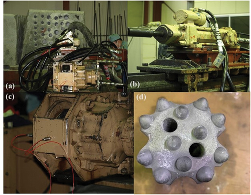
We applied the methods proposed by Senjoba et al. [20] to the proposed rock-identification system. The drilling experiment was conducted using a YH-70 stationary drifter (Yamamoto Rock Machine Ltd, Tokyo, Japan) with a rotary percussion drilling method (Figure 1a,b). The drifter contained a piston and motor inside, which served as a power source for the striking and rotational forces. These forces were transmitted to the rod, which secured the drilling length and straight drill hole. A bit was attached to the rod to interact with the drilling surface. In this study, a tungsten carbide drill bit was used to drill two types of rocks (Figure 1d), granite and marble, with uniaxial compression strengths of 117 and 105 MPa, respectively. The dimensions of both rocks were approximately 4.2 m³ with a drilling surface area of 2.61 m². The impact pressure, striking frequency, rotation pressure, and the number of hits per minute were 13.5–13.7, 52 Hz, 4–6 MPa, and 3120, respectively. Holes 1 m in length were drilled for 60 seconds in each rock. A piezoelectric acceleration transducer (600 series; TEAC Corporation, Tokyo, Japan) was mounted on the guide cell of the rock drifter facing the drilling direction to measure drill vibrations in the longitudinal direction. The accelerometer had a sensitivity of 0.04 ± 20% pc/m/s², a transverse sensitivity of 5%, and a frequency response range of 1.6 Hz–50 kHz. In drilling operations, vibration frequencies can reach several kilohertz. Therefore, a sampling frequency of 50 kHz was chosen for all experiments to ensure the accurate capture of a wide range of vibration signals, including crucial high-frequency components necessary for rock type identification. According to the Nyquist theorem, the sampling frequency should be at least twice the highest frequency present in the signal to avoid aliasing [21]. By setting the sampling frequency at 50 kHz, it allows for sufficient sampling and analysis of the relevant frequency components. Using the accelerometer, vibration data were transmitted to an NR-500 series data logger (Keyence, Itasca, IL, USA) with a built-in amplifier. The information was saved on a personal computer as comma-separated values (CSV) files.

Figure 1. Experimental setup and equipment used for data collection; (a) experimental setup, (b) rotary percussion rock drifter, (c) accelerometers mounted on the guide cell of the rock drifter, and (d) tungsten carbide tapered drill bit used for drilling.

2.2. Data preprocessing

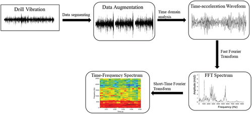
Signal segmentation was carried out to improve the computational efficiency and temporal resolution of the signals. This process involves dividing signals into distinct segments. The waveform of one drill hole was 60 seconds long and had 3,000,000 data points, divided into 0.06 seconds segments, each segment formed a data window containing 3,000 data points with no overlapping. This ensured that each segmentation signal contained at least three drill-bit hits. Using larger window sizes allows for more data to be processed, but increases the complexity of the model, whilst shorter windows simplify the model’s complexity, making it easier for the model to learn and generalise from the data. Approximately 1000 segments were obtained from one drill hole. After data segmentation, each rock contained 7,147 data samples. Thereafter, the time-domain data segments were converted into frequency domain using FFT. This conversion helps in revealing the frequency components of the signals. The analysis is further expanded by utilising the Short-Time Fourier Transform (STFT), which allows for time-frequency analysis. This is essential in understanding how the frequency content of the signal evolves over time. By applying FFT and STFT, we can analyse the drill vibration signals in both the time and frequency domains. This enables us to identify different rock types based on their distinctive spectral characteristics. Figure 2 illustrates the data preprocessing technique used in this study.

Figure 2. Data preprocessing technique. The drill vibrations were augmented to increase the number of samples. Fast Fourier transform (FFT) was used to transform the augmented segments into the frequency domain and short time–frequency transform was used to acquire the time–frequency spectra.

3. Signal analysis

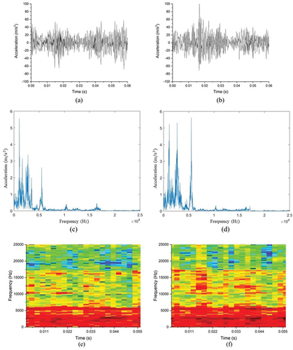
Several studies have shown that it is possible to identify different rocks by performing signal analysis as there is a correlation between rock properties and the vibration signal of the rock drill operation [8–10]. Hence, the time-domain waveforms, frequency spectra, and time–frequency spectra of each rock were analysed. Figure 3 shows the time-series waveforms, frequency spectra, and spectrogram comparisons of the two rocks. The acceleration of the time-series for granite rock oscillated between −80 m/s² and 80 m/s², whereas it was between −100 m/s² and 100 m/s² for marble rock (Figure 3a,b). On average, granite has a smaller amplitude than marble. Based on the time-series analysis, it was concluded that it was possible to distinguish the two rocks. Subsequently, the frequency spectra of the two rocks were analysed. The corresponding spectra are shown in (Figure 3c,d). Generally, it was observed that both rocks had similar dominant frequencies, in the range of 0–6,000 Hz. The dominant frequency peaks of granite were lower than those of marble rock. In a study by Khoshouei et al. [22], it was concluded that the dominant frequencies of igneous rocks are usually greater than those of metamorphic rocks and those of metamorphic rocks are greater than those of sedimentary rocks, owing to the particle composition of these rocks. Based on the comparison of the dominant frequency peaks of each rock, a distinction can be made to identify the two rocks. STFT was used to understand the frequency variations of the signal over time. (Figure 3e,f) show spectrograms of the two rocks. The spectrograms further confirmed that the dominant frequencies of both rocks were in the range of 0–6,000 Hz. Both rocks exhibited similar frequency behaviours over time. The intensities of the frequencies were stable across the time intervals because the vibration signals were stationary. Although the process of signal analysis is dependable, it is tedious; hence, a deep-learning approach is needed.

Figure 3. Conventional signal analysis results from (a) the granite rock time-acceleration waveform, (b) marble rock time-acceleration waveform, (c) granite rock frequency spectrum, (d) marble rock time–frequency spectrum, (e) granite rock time–frequency spectrum, and (f) marble rock time–frequency spectrum.

4. Proposed approach for rock identification using deep learning

The CNN is a powerful machine-learning method applied in different fields. It is a type of feed-forward ANN with a data-processing structure characterised by local receptive fields and sparse connections between layers. CNNs can be trained to automatically extract hierarchical features in input data through their processing layers while exhibiting high computational efficiency in image processing compared to other CNN variants. Peng et al. [23] established that CNNs can learn more robust features with better generalisation performance and save training costs through weight sharing and pooling operations, compared with traditional fully connected neural networks. A typical CNN is composed of an input layer, multiple convolutional and pooling layers, fully connected layers, and an output (classification) layer [24]. The input layer introduces the data into the system, from there the kernels perform convolution operations on the time series of the preceding layer. The convolution stride, the filter numbers, and the size of the kernels are some of the parameters to be determined depending on domain knowledge or experiments. The Pooling layer feature map is divided into equal-length segments, and then every segment is represented by its average or maximum value. The advantage of the pooling operation is downsampling the convolutional output bands, thus reducing variability in the hidden activations. After several convolution and pooling operations, the original time series is represented by a series of feature maps. All the feature maps are connected to generate a long new time series as the final representation of the original input which is fully connected via weights to the output layer. The values from the fully connected layers are transferred to a non-linear activation function such as the softmax layer, which returns the probability of each class. The output layer has n neurons, corresponding to n classes of the time series [25]. The weights and biases are learned during the training process using the stochastic gradient descent method whilst the gradients are computed by the backpropagation method [20].

Over the years, CNNs have achieved successful results in image recognition tasks. CNNs can provide excellent classification performance; however, the parameters inside the models are inexplicable owing to the black-box nature of neural networks. Using explainable AI, CNNs can be made transparent and insightful for humans. Gradient-weighted Class Activation Mapping (Grad-CAM) is a technique for producing ‘visual explanations’ for decisions from a large class of CNN-based models, making them more transparent and explainable. Grad-CAM uses the gradients of any target concept flowing into the final convolutional layer to produce a coarse localisation map, highlighting important regions in the image for predicting the concept [26]. Equation 1 represents the Grad-CAM operation. ‘First, the gradient $\frac{\mathrm{\partial }{y}^c}{\mathrm{\partial }{A}^k}$of the score $y^c$ for class c before the final soft-max layer is computed for the feature map activation $A^k$ of convolution k from the deepest convolutional layer. Then, the backpropagated gradients are globally max-pooled to yield the importance of the convolution for the class, ${\alpha }_k^c$: this is called the neuron importance weight. Finally, a localisation map $L^c$ is obtained by computing the weighted sum, followed by a ReLU, to obtain only positive contributions’ [27].

(1) $L^c=\mathit{ReLU}\left(\sum _k{\alpha }_k^c{A}^k\right)$(1)

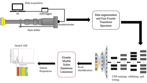
By observing and analysing attention maps, CNN models can be explained and verified. Figure 4 shows a flowchart of the proposed rock-identification system. Accelerometers are mounted on the rock drifter to capture drill vibration data. Afterwards, data segmentation and Fast Fourier Transformation are performed to obtain frequency spectrum images. These frequency spectrum images are then used as input for training and testing a convolutional neural network (CNN) algorithm. Finally, Gradient-weighted Class Activation Mapping (Grad-CAM) is applied to explain the network’s predictions.

Figure 4. Overview of the proposed lithology identification system.

4.1. Comparison of neural networks

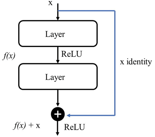
The CNN architecture influences computational efficiency, memory space, and model accuracy. As various CNNs perform differently on the same dataset, it is important to compare different CNN structures and select the best one [28]. ResNet-50 extends neural networks to extremely deep structures by adding shortcut connections to each residual block, to enable a gradient flow directly through the bottom layers. Figure 5 shows a residual block in a ResNet-50 model. By adding the shortcut connections, the output of a layer is transformed from H(x)=f(x) to H(x)=f(x)+x, where H (x) refers to the layer’s output, f () is the activation function and x is the input. It is easy to optimise the entire model as the shortcut connections decrease the model’s computational complexity and number of parameters [29].

Figure 5. Residual block of ResNet-50 models. The Rectified Linear Unit (ReLU) activation function is applied within the residual block.

Inception-v3 [30] is another CNN model that is 42 layers deep and much wider than other CNNs. Multiple filters of different sizes are used at the same level. It is composed of symmetric and asymmetric building blocks. The architecture consists of convolutions, average pooling, max pooling, concatenations, dropouts, and fully connected layers. There are various series of inception networks, and experiments [31] have shown that the structure of Inception-v3 is superior to those of other versions. Inception-v3 models are optimised by factorised convolutions, regularisation, dimension reduction, and parallelised computations. The convolutions are factorised by replacing one 5 × 5 convolution with two 3 × 3 convolutions, as a way of reducing the number of parameters in the model [30].

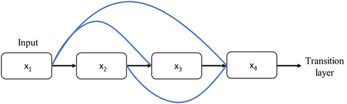
The final model considered in this study was DenseNet-201, which was 201 layers deep. In a traditional CNN model, images pass through several convolutions to obtain high-level features, a network with L layers has L connections; one between each layer and its subsequent layer; however, a dense network has $\frac{L\left(L^2+1\right)}{2}$ direct connections, each layer obtains feature maps from all preceding layers, making the network thinner and more compact. According to Huang et al. [31] the model achieves higher computational and memory efficiency owing to its dense blocks and connections, which eliminates the vanishing gradient problem [31]. Figure 6 illustrates the layout of a dense block.

Figure 6. A four-layer dense block. In each layer, the feature maps of all preceding layers are used as inputs, and the feature maps of that layer are used as inputs to all subsequent layers.

4.2. Network training and implementation details

All the models were trained with the same parameter settings: data splitting, learning rate, batch size, and number of epochs. The models were then evaluated using classification accuracy as a performance metric. The 7147 images from each rock sample were randomly split into 5147 training sets, 1000 validating sets, and 1000 testing sets using the hold-out cross-validation method. The training process was performed using MATLAB R2020b with a deep-learning toolbox on a workstation with a Windows 10, 64-bit operating system, an Intel Core i7-8750 H CPU @ 2.2 central processing unit, 16 Gb memory, and an NVIDIA GeForce GTX graphics processing unit. The hyperparameters listed in Table 1 were used to maintain consistency across all experiments.

Table 1. Experimental implementation details.

Hyperparameters	Value
Optimization algorithm	Adaptive moment estimation (ADAM)
Learning rate	0.001
Loss function	Cross entropy
Epochs	5
Batch size	8

5. Results

A comparative study of three machine-learning algorithms ResNet-50, Inception-v3, and DenseNet-201 was conducted to evaluate which model could better distinguish rocks based on frequency spectrum images. Table 2 lists the training and validation accuracies, number of parameters, and computational efficiencies of the three CNN models. Training and validation accuracies were used to measure the performance of the models. All models performed well, as there was a marginal difference between the validation and training accuracies. ResNet-50, Inception-v3, and DenseNet-201 had an accuracy value of 100% on the training dataset and that of 96.70%, 99.10%, and 97.780%, respectively, on the validation dataset. Notably, there was no overfitting observed, as the training and validation accuracies were consistent. Table 2 shows that DenseNet-201 had the lowest number of parameters and the shortest training time of 173 min, while ResNet-50 had 23.5 million parameters and a training time of 283 min. The Inception-v3 model required the most training time, using 21.8 million parameters in 332 min. By assessing the loss curves of the three models shown in Figure 7, it can be observed that the ResNet-50 model demonstrated a stable loss curve throughout most of the training process. Although a few disturbances were observed towards the end of training. Inception-v3 had a fluctuating loss curve at the initial stages of training. However, as training progressed, the loss converged to a steady state. DenseNet-201 exhibited a volatile loss curve at approximately 500–700 iterations.

Figure 7. Training loss curve for the ResNet-50, Inception-v3, and DenseNet-201 models.

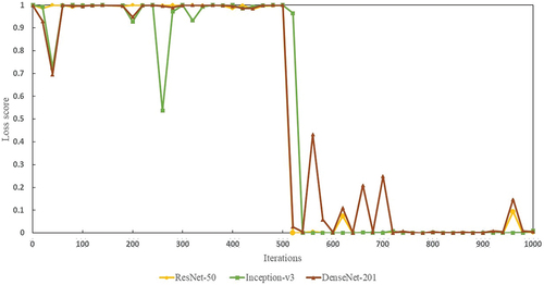
Table 2. Experimental implementation details.

Model	Training accuracy (%)	Validation accuracy (%)	Number of parameters	Computation time (min)
ResNet-50	100	96.70	23.5 M	283
Inception-v3	100	99.10	21.8 M	332
DenseNet-201	100	97.80	18.1 M	173

The classification accuracy was used as a metric to assess the performance of the models on unseen test data. Unseen test data demonstrates the model’s ability to handle real-world data that extends beyond its training scope. This metric calculates the percentage of samples that are correctly classified. Equation 2 represents the accuracy metric:

(2) $\mathit{Accuracy}=\frac{\mathit{TP}+\mathit{TN}}{\mathit{TP}+\mathit{TN}+\mathit{FP}+\mathit{FN}}$(2)

where TP (true positive) refers to samples correctly classified as positive, TN (true negative) refers to those correctly classified as negative, FP (false positive) refers to those misclassified as positive, and FN (false negative) refers to those misclassified as negative.

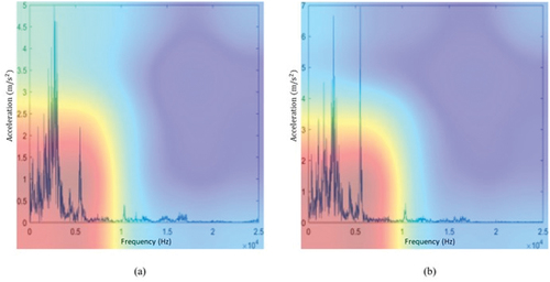
Figure 8 shows the confusion matrix obtained for each model. These represent the predicted results for the test set. Using the confusion matrix, the TN, FN, FP, TP, and classification accuracies can be easily assessed. All models achieved a classification accuracy higher than 95%. Inception had the highest classification accuracy of 99.0%, followed by ResNet-50 with 98.4%, and DenseNet-201 with 97.4%. From the confusion matrices and Figure 9, it is evident that the ResNet-50 model had a marginally higher number of misclassified granite rocks, and 14 frequency spectra were misidentified. Marble was the most misclassified rock using DenseNet-201, with 18 misclassifications. Inception-v3 was considered the best model. To gain insight into the decision-making of the Inception-v3 model, the Grad-CAM algorithm was used to highlight the noteworthy frequencies and accelerations responsible for a given prediction. Figure (10a,b) show the attention maps produced using Grad-CAM. The high-attention area is shown in orange, whereas the low-attention area is shown in blue. To predict both rocks, the model focused on a frequency range of 0–8,000 Hz. This indicates that the model identifies the most distinct characteristics within this frequency band. There was no correlation observed between the acceleration peaks.

Figure 8. Confusion matrices showing the classification results of the three models on test data. The x-coordinate shows the target class, while the y-coordinate shows the output class. The overall classification accuracy is denoted by the yellow square; (a) ResNet-50’s confusion matrix, (b) Inception-v3’s confusion matrix, and (c) DenseNet-201’s confusion matrix.

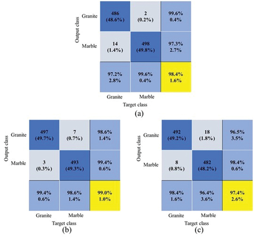
Figure 9. Misclassified examples for the three models.

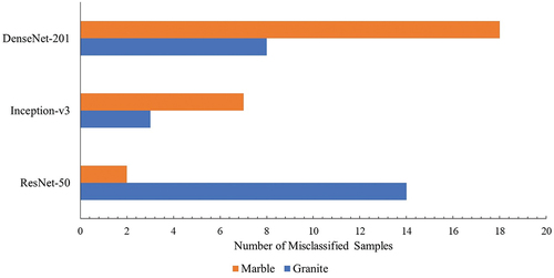
Figure 10. Heatmaps of Gradient-weighted Class Activation Mapping (Grad-CAM) from the Inception-v3 model. It highlights important frequencies for predicting rock samples. The high-attention and low-attention region is indicated by orange-yellow and blue color, respectively. (a) Granite rock, and (b) Marble rock. Note: For optimal interpretation, color versions of these Figures should be used, as the heatmaps may not reproduce well in greyscale or photocopied versions.

6. Discussion

An investigation was completed to compare three machine learning algorithms: ResNet-50, Inception-v3, and DenseNet-201, with the aim of assessing their abilities in differentiating rocks using frequency spectrum images. The aim was to analyse the model’s trade-offs in terms of accuracy, computational efficiency, and memory usage.

Inception-v3 consistently demonstrated a competitive edge in terms of validation and classification accuracies; 99.10% and 99.0% respectively. Its complex architecture and utilisation of multiple inception modules allowed it to capture intricate patterns within the frequency spectrum images. ResNet-50 and DenseNet-201 models also exhibited high validation and classification accuracies; however, the DenseNet-201 model exhibited a volatile loss curve due to its densely connected layers and the vanishing gradient problem associated with training deep networks. ResNet-50 emerged as the most computationally efficient model among the three. Its skip connections facilitated the training of deeper networks with fewer computations in each layer, contributing to faster convergence. Inception-v3’s complex architecture led to longer training times, increased computational demands, and memory requirements. This could be a potential drawback when deploying the model on resource-constrained devices. In contrast, ResNet-50 and DenseNet-201 demonstrated more memory-friendly performance, making them suitable choices for applications where memory constraints are critical. The selection of the most appropriate model depends on the specific task requirements and available resources, emphasising the importance of considering these trade-offs during model selection and deployment.

The Inception-v3 model was selected as the optimal model due to its notably high accuracy, fewer instances of misclassification, and steady convergence, despite the extended training time. The proposed method introduces a low-latency technique for rock identification, as deep-learning models can process large amounts of data faster and more efficiently. This system has the potential to enhance efficiency in rock identification by leveraging the speed and capacity of deep learning models. Our findings concerning the application of deep learning in rock identification complement the work of Chen et al. [32], who used time–frequency images from drill string vibration data as inputs for CNN models. The findings of Chen et al. [32] showed that machine-learning algorithms provide a superior and time-efficient method for lithology identification. Another study by Xie et al. [17] confirmed the importance of machine-learning algorithms in formation lithology identification. However, the study used well-log data as input to machine-learning algorithms, with substantial data preprocessing techniques. The proposed study offers a minimal data preprocessing procedure and a single input parameter, making it more efficient, and because drill vibrations are more readily available during drilling than well-log data, the method can be easily implemented in real-time.

Furthermore, with the application of Grad-CAM, we identified the noteworthy frequencies of the two rocks. Yoo and Jeong [33] established that Grad-CAM can be used as an alternative method for vibration analysis. The results of this study indicated that the model focused on frequencies ranging from 0 to 8,000 Hz for both rocks. However, it was found that the dominant frequencies and acceleration peaks of each rock were difficult to distinguish from one another. This could be due to the fact that both Marble and granite rocks exhibit overlapping frequency responses within the 0–8,000 Hz range, making it challenging to visually differentiate between them. The results of this analysis are comparable with those of the signal analysis method, demonstrating that the CNN model was able to extract salient characteristics from the drill vibrations of the two rocks. This is supported by a study performed by Qin et al. [34], who indicated that a frequency range of 0–25,000 Hz can be used as distinguishable characteristics for pattern recognition in lithology. Kumar et al. [16] also established that dominant acoustic frequencies between 4,000 and 9,000 Hz can be used to estimate rock properties during diamond core drilling.

7. Conclusion

This study introduces an economical, automated, and no-feature selection rock identification system that uses drill vibration. The approach involves minimal data preparation and relies on one input parameter. This eliminates the need for resource-intensive feature extraction and complex computations, resulting in a more efficient alternative that can be implemented in real-time compared to previous studies and conventional methods presently employed in the industry. The main conclusions are as follows:

1. Signal analysis was performed to distinguish rock samples. A comparative study of the signals was performed in the time, frequency, and time–frequency domains. The results indicated that the time-series waveforms and frequency spectra of each rock were distinct and can be used to classify the two rocks. Both rocks had dominant frequencies ranging from 0 Hz to 6,000 Hz, and the dominant frequency peaks of granite were lower than those of marble. The results showed that it is not possible to differentiate rock samples using time–frequency spectra.

2. The ResNet-50, Inception-v3, and DenseNet-201 algorithms were used to build rock-identification models. The frequency spectrum images were used as inputs for the CNN algorithms. In terms of accuracy, the Inception-v3 model demonstrated the highest precision achieving a classification accuracy of 99.0%. This accomplishment highlights the model’s ability to automatically abstract high-level features from spectral images.

3. The Grad-CAM algorithm was applied to automatically detect the dominant frequencies used by the Inception-v3 model to classify rock samples. The investigation showed that frequency ranges of 0–8,000 Hz are important for rock classification in this case. This verified that the Inception-v3 model was focusing on salient frequencies when classifying the rocks.

The proposed approach identifies rocks at high speed, high precision, and because deep learning can process large amounts of data in a time and cost-effective manner, this could increase productivity by facilitating immediate adjustments to drilling strategies, ensuring that the drilling process is optimised for the encountered geological conditions. The system can aid in choosing the appropriate drilling techniques, equipment, and tools. In this study, we considered only two rock samples, which limits generalising the results. More rock samples may be evaluated in the future to reach more comprehensive conclusions. Finally, as the mining field embraces mining 4.0, to optimise safety, sustainability, productivity, and efficiency, there is a need to integrate deep learning into mining operations and to present a capable system for identifying rocks during drilling operations in real time.

CrediT statement

Lesego Senjoba: Conceptualisation, Methodology, Software, Formal analysis, Writing- original draft, writing-review & editing. Hajime Ikeda: Investigation, writing-review & editing. Hisatoshi Toriya: Software, Project administration. Tsuyoshi Adachi: Supervision, Resources. Youhei Kawamura: Supervision, Conceptualisation, writing-review & editing, Validation.

Acknowledgments

The authors would like to express their gratitude to Mitsubishi Materials Corporation for their assistance with data collection.

Disclosure statement

No potential conflict of interest was reported by the author(s).

Additional information

Funding

This study did not receive any specific grants from funding agencies in the public, commercial, or non-profit sectors.

References

- R. Ghosh, Assessment of Rock Mass Quality and Its Effects on Charge Ability Using Drill Monitoring Technique, Luleå University of Technology, Luleå, 2017.
- D.V. Ellis, Well Logging for Earth Scientists, 2nd ed. Springer, Dordrecht, The Netherlands, 2007.
- V. Isheyskiy and J.A. Sanchidrián, Prospects of applying MWD technology for quality management of drilling and blasting operations at mining enterprises, Minerals 10 (10) (2020), pp. 925. doi:10.3390/min10100925.
- Z. Li, K. Itakura, and Y. Ma, Survey of measurement-while-drilling technology for small-diameter drilling machines, Electron. J. Geotechnical. Eng. 19 (n.d), pp. 17.
- V. Vezhapparambu, J. Eidsvik, and S. Ellefmo, Rock classification using multivariate analysis of measurement while drilling data: Towards a better sampling strategy, Minerals 8 (9) (2018), pp. 384. doi:10.3390/min8090384.
- R. Leung and S. Scheding, Automated coal seam detection using a modulated specific energy measure in a monitor-while-drilling context, Int. J. Rock Mech. Min. Sci. 75 (2015), pp. 196–209. doi:10.1016/j.ijrmms.2014.10.012.
- S. Manzoor, Rock mass characterization using MWD data and photogrammetry, in Mining Goes Digital C. Mueller, ed. 1st ed. CRC Press, London, 2019, pp. 217–225. doi: 10.1201/9780429320774-25.
- M. Zborovjan and I. Leššo, Acoustic identification of rocks during drilling. Acta Montan. Slovaca. 8 (2003), pp. 3.
- S. Shreedharan, C. Hegde, S. Sharma, and H. Vardhan, Acoustic fingerprinting for rock identification during drilling, IJMME 5 (2) (2014), pp. 89. doi:10.1504/IJMME.2014.060193.
- M. Khoshouei and R. Bagherpour, Predicting the geomechanical properties of hard rocks using analysis of the acoustic and vibration signals during the drilling operation, Geotech. Geol. Eng. 39 (3) (2021), pp. 2087–2099. doi:10.1007/s10706-020-01611-z.
- B.B. Sinaice, Y. Kawamura, J. Kim, N. Okada, I. Kitahara, and H. Jang, Application of deep learning approaches in igneous rock hyperspectral imaging. In: E. Topal, ed. Proceedings of the 28th International Symposium on Mine Planning and Equipment Selection - MPES 2019, Springer Series in Geomechanics and Geoengineering, Springer International Publishing, Cham, 2020, pp. 228–235. doi:10.1007/978-3-030-33954-8_29.
- Z. Xu, W. Ma, P. Lin, H. Shi, D. Pan, and T. Liu, Deep learning of rock images for intelligent lithology identification, Comput. Geosci. 154 (2021), pp. 104799. doi:10.1016/j.cageo.2021.104799.
- dos Anjos, CEM, M.R.V. Avila, A.G.P. Vasconcelos, A.M. Pereira Neta, L.C. Medeiros, A.G. Evsukoff, R. Surmas, and L. Landau, Deep learning for lithological classification of carbonate rock micro-CT images, Comput. Geosci. 25 (3) (2021), pp. 971–983. doi:10.1007/s10596-021-10033-6.
- D. Li, R. Shirani Faradonbeh, A. Lv, X. Wang, and H. Roshan, A data-driven field-scale approach to estimate the permeability of fractured rocks, Int. J. Min. Reclam. Environ. 36 (10) (2022), pp. 671–687. doi:10.1080/17480930.2022.2086769.
- B. Yu, D. Zhang, B. Xu, Y. Liu, H. Zhao, and C. Wang, Modeling of true triaxial strength of rocks based on optimized genetic programming, Appl. Soft Comput. 129 (2022), pp. 109601. Available at. 10.1016/j.asoc.2022.109601.
- C. Kumar, H. Vardhan, C. Murthy, and N.C. Karmakar, Estimating rock properties using sound signal dominant frequencies during diamond core drilling operations, J. Rock Mech. Geotech. Eng. 11 (4) (2019), pp. 850–859. doi:10.1016/j.jrmge.2019.01.001.
- Y. Xie, C. Zhu, W. Zhou, Z. Li, X. Liu, and M. Tu, Evaluation of machine learning methods for formation lithology identification: A comparison of tuning processes and model performances, J. Pet. Sci. Eng. 160 (2018), pp. 182–193. doi:10.1016/j.petrol.2017.10.028.
- Y. Imamverdiyev and L. Sukhostat, Lithological facies classification using deep convolutional neural network, J. Pet. Sci. Eng. 174 (2019), pp. 216–228. doi:10.1016/j.petrol.2018.11.023.
- X. Hu, L. Chu, J. Pei, W. Liu, and J. Bian, Model complexity of deep learning: A survey, Knowl. Inf. Syst. 63 (10) (2021), pp. 2585–2619. doi:10.1007/s10115-021-01605-0.
- L. Senjoba, Y. Kosugi, M. Hisada, and Y. Kawamura, Lithology identification during rotary percussion drilling based on acceleration waveform 1D convolutional neural network, in Rock Mechanics and Engineering Geology in Volcanic Fields, CRC Press, London, 2022, pp. 435–441. doi:10.1201/9781003293590-54.
- A. Lesne, The discrete versus continuous controversy in physics, Math. Struct. Comp. Sci. 17 (2) (2007), pp. 185–223. doi:10.1017/S0960129507005944.
- M. Khoshouei, R. Bagherpour, and M.H. Jalalian, Rock type identification using analysis of the acoustic signal frequency contents propagated while drilling operation, Geotech. Geol. Eng. 40 (3) (2022), pp. 1237–1250. doi:10.1007/s10706-021-01957-y.
- D. Peng, Z. Liu, H. Wang, Y. Qin, and L. Jia, A novel deeper one-dimensional CNN with residual learning for fault diagnosis of wheelset bearings in high-speed trains, IEEE. Access 7 (2019), pp. 10278–10293. doi:10.1109/ACCESS.2018.2888842.
- J. Grezmak, P. Wang, C. Sun, and R.X. Gao, Explainable convolutional neural network for gearbox fault diagnosis, Procedia. CIRP 80 (2019), pp. 476–481. doi:10.1016/j.procir.2018.12.008.
- B. Zhao, H. Lu, S. Chen, J. Liu, and D. Wu, Convolutional neural networks for time series classification, J. Syst. Eng. Electron. 28 (1) (2017), pp. 162–169. doi:10.21629/JSEE.2017.01.18.
- D. Cian, J. van Gemert, and A. Lengyel, Evaluating the performance of the LIME and Grad-CAM explanation methods on a LEGO multi-label image classification task, arXiv: 2008.01584 [cs]. (2020), [Preprint]. http://arxiv.org/abs/2008.01584.
- R.R. Selvaraju, M. Cogswell, A. Das, R. Vedantam, D. Parikh, and D. Batra, Grad-CAM: Visual explanations from deep networks via gradient-based localization, Int. J. Comput. Vis. 128 (2020), pp. 336–359. doi:10.1007/s11263-019-01228-7.
- F. Chen and J.Y. Tsou, Assessing the effects of convolutional neural network architectural factors on model performance for remote sensing image classification: An in-depth investigation, Int. J. Appl. Earth Obs. Geoinf. 112 (2022), pp. 102865. doi:10.1016/j.jag.2022.102865.
- K. He, X. Zhang, S. Ren, and J. Sun, Deep residual learning for image recognition, Proceedings of the IEEE Conference on Computer Vision and Pattern Recognition (CVPR), Las Vegas, NV, USA, 2016, pp. 770–778.
- C. Szegedy, V. Vanhoucke, S. Ioffe, J. Shlens, and Z. Wojna, Rethinking the inception architecture for computer vision, Proceedings of the IEEE Conference on Computer Vision and Pattern Recognition (CVPR), Las Vegas, NV, USA, 2016, pp. 2818–2826.
- G. Huang, Z. Liu, L. van der Maaten, and K.Q. Weinberger, Densely connected convolutional networks, Proceedings of the IEEE Conference on Computer Vision and Pattern Recognition (CVPR), Honolulu, HI, USA, 2017, pp. 4700–4708.
- G. Chen, M. Chen, G. Hong, Y. Lu, B. Zhou, and Y. Gao, A new method of lithology classification based on convolutional neural network algorithm by utilizing drilling string vibration data, Energies 13 (4) (2020), pp. 888. doi:10.3390/en13040888.
- Y. Yoo and S. Jeong, Vibration analysis process based on spectrogram using gradient class activation map with selection process of CNN model and feature layer, Displays 73 (2022), pp. 102233. doi:10.1016/j.displa.2022.102233.
- M. Qin, K. Wang, K. Pan, T. Sun, and Z. Liu, Analysis of signal characteristics from rock drilling based on vibration and acoustic sensor approaches, Appl. Acoust. 140 (2018), pp. 275–282. doi:10.1016/j.apacoust.2018.06.003.