
Abstract
In this paper, we study the dynamics behaviour of a stratum of plant–herbivore which is modelled through the following F(x, y)=(f(x, y), g(x, y)) two-dimensional map with four parameters defined by
where x≥0, y≥0, and the real parameters a, b, r, k are all positive. We will focus on the case a≠b. We study the stability of fixed points and do the analysis of the period-doubling and the Neimark–Sacker bifurcations in a standard way.
Introduction
The dynamics of a discrete-time mathematical model arises in a variety of applications especially in ecology and mathematical biology and is still a current topic of research. In ecology, predator–prey or plant–herbivore models can be formulated as discrete-time models. A plant–herbivore model (which is also of host–parasite type) applies to study the interaction between a plant species and a herbivore species. Discrete models described by difference equations for interacting populations are of considerable interest to biologists and agricultural ecologists. These models are actually more reasonable than the continuous-time models when populations have non-overlapping generations. This certainly happens for a population that has a one-year life cycle, such as insects. For example, gypsy moth larvae hatch from the egg mass after bud-break and feed on new leaves. At the end of the season, adult gypsy moths lay eggs and die. The gypsy moth is a notorious forest pest in North Central USA whose outbreaks are almost periodic and cause significant damage to the infested forests. A discrete-time model can exhibit more plentiful and hence more complicated dynamical behaviours than a continuous-time model of the same type. Jing and Yang [Citation16] and Liu and Xiao [Citation19] remarked that discrete-time prey–predator models have more complicated dynamics than those in continuous models.
In recent years, a significant number of published papers have been on mathematical models in biology. Mathematical models on prey–predator systems have created a major interest during the last few decades. Study of such systems with discrete- and continuous-time models can be found in [Citation1,Citation4,Citation8,Citation11–15,Citation17,Citation19].
Summers and colleagues [Citation7] have analysed four typical discrete-time ecosystem models under the effects of periodic forcing. They observed that periodic forcing can produce a chaotic dynamics. Agiza et al. [Citation2] found chaotic dynamics of a discrete prey–predator model with Holling's Type II response function. They did not consider the natural death rate of the predators. Kang and colleagues [Citation4] observed quasi-periodicity, period-doubling and chaos in plant–herbivore interaction in the form of a host–parasite model. It is observed that the continuous model of such a system shows global stability of an interior equilibrium point.
Discrete-generation host–parasite models of the general form
The simplest version of this model is that of Nicholson–Bailey [Citation5]:
Beddington et al. [Citation6] considered an extension of the Nicholson–Bailey host–parasite model:
In order to have a more realistic model, one can consider the system
In the case b=a, this is the density-dependent predator–prey model studied by Beddington et al. [Citation6]. By choosing an appropriate family chart (a parameter-dependent family of coordinate changes), one can assume b=r, and then the behaviour of the two populations just depends on the three positive parameters a, r and k. This system has the advantage that the dynamics restricted to is given by the Ricker difference equation
, so the growth of the prey is limited and does not become unbounded.
Density-dependent models of the general form
The existence of a Neimark–Sacker bifurcation in the model implies that both the host and parasite populations can oscillate around some mean values, and that these oscillations are stable and will continue indefinitely under suitable conditions.
It is proved in [Citation12] that system (11) and (12) has a non-trivial steady-state solution which is stable for a certain range of parameter values, which is explicitly determined, and also undergoes a Neimark–Sacker bifurcation that produces an attracting invariant curve in some areas of the parameter space and a repelling one in others.
A general plant–herbivore model of the form
Assumption 1 Pn represents the biomass of the plant population (nutritious) after the attacks by the herbivore but before its defoliation. Hn represents the biomass of the herbivore population before they die at the end of the season n.
Assumption 2 Without the herbivore, the biomass of the plant population follows the dynamics of the Ricker model [Citation21], namely
Assumption 3 It is supposed that the herbivores search for food randomly. The leaf area consumed is measured by the parameter a, i.e. a is a constant that correlates the total amount of the biomass that an herbivore consumes. The herbivore has a one-year life cycle, the larger the a, the faster is the feeding rate.
Assumption 4 After attacks by herbivores, the biomass in the plant population is reduced to a fraction of that present in the absence of herbivores. Hence,
Assumption 5 The amount of decreased biomass in the plants is converted to the biomass of the herbivore. It is assumed that the biomass conversion constant c is 1. Therefore, at the end of the season n, one has that
The bifurcation diagram in the parameter space of Equations (13) and (14) was presented by Armbruster et al. [Citation4]. Two control strategies are suggested in [Citation4]: reducing the population of the herbivore under some threshold and increasing the growth rate of the plant leaves.
Our paper is organized as follows. In Section 2, we give a brief discussion on the model under consideration. Fixed points and their stability are discussed in Section 3. Bifurcations analysis of the model is performed in Section 4.
2. Model
Consider the following two-dimensional map with four parameters defined by
In this paper, we study the stability of fixed points and do the analysis of the period-doubling and the Neimark–Sacker bifurcations in a standard way. Using an appropriate rescaling , we can without loss of generality suppose that b=r>0 and a≠r. One can, of course, choose another family chart which permits to take b=1 and a≠1. For convenience, we prefer here to take b=r and a≠r. In that case, we can have at most three fixed points at
, where
and y* is the unique positive solution of
Also we have the following estimates on x*, y*:
Let
Then the interior equilibria are the intersection points of the functions f1 and f2 in the first quadrant. In addition, we have the following observations: f1(0)=0, ,
; f2(0)=0,
,
;
for y∈(0, 1) and a≤1/k while it has a unique zero at some y∈(0, 1) when a>1/k; and that
Thus if ak>1, then F(y)>0 for 0<y≪1 and if ak≤1, then F(y)<0 for 0<y≪1. Hence, the intersection of f1(y) and f2(y) in the first quadrant has 1 () or 0 () positive fixed point depending on the sign of ak−1. Therefore, we have the following propositions:
Figure 1. Graph of the functions f1 and f2 in the case 0<a≤1/k.
Figure 2. Graph of the functions f1 and f2 in the case a>1/k.
Proposition 2.1
For any r>0 and 0<a≤1/k, system (17) has no positive fixed points ().
Proposition 2.2
For any r>0 and a>1/k, system (17) has a unique positive fixed point ().
Now we turn to investigate the stability of system (17) by taking b=r and a≠r.
3. Stability of fixed points
In this section, we study the stability of fixed points via linearization, namely using the linear part of Equation (16) evaluated at each fixed point. To this end, we need the partial derivatives of f and g, which are as follows:
Since , then the Jacobian matrix at the origin is
Hence, the extinction fixed point (0, 0) is a saddle point. This implies that plants cannot die out. It is noted that the lines and
are invariant under the dynamics of Equation (16) such that
is the stable manifold of the origin (0, 0) and
denotes the unstable manifold. The map restricted to
is the Ricker map given by
It is noted that the Schwartz derivative of the Ricker map R(x) defined in Equation (19) at x=k is calculated as follows:
This derivative is negative provided that r≠1. Since for r=2 we have and
, in this case, by the well-known arguments, any trajectory with the initial condition (x0, 0) on the x-axis with x0>0 goes towards the exclusion fixed point (k, 0). To obtain the Jacobian matrix at the exclusion fixed point (k, 0), we have that
The eigenvalues of the above matrix are given by and
. Depending on the location of the eigenvalues in the complex plane w.r.t. the unit circle, we have the following statements on (k, 0):
Proposition 3.1
The following hold.
If ak<1 and 0<r<2, then it is an attracting node.
If ak<1 and r>2, then it is a saddle point.
If ak>1 and r>2, then it is a repelling node.
If ak>1 and 0<r<2, then it is a saddle point.
Proof The proof is straightforward. For example, if ak<1 and 0<r<2, then and
; hence, we have a stable node at (k, 0).
Proposition 3.2
When ak=1 and 0<r<2, we have a non-hyperbolic fixed point at (k, 0), which is unstable.
Proof In the case ak=1 and 0<r<2, we compute below the centre manifold at (k, 0) and the dynamics restricted to the centre manifold to determine the orbit structure near (k, 0) in the first quadrant . First, we bring the fixed point (k, 0) to the origin by using a linear translation, i.e.
. This yields the following
two-dimensional map with two parameters defined by
Next, we put the linear part of Equation (21) in Jordan normal form by using the linear transformation
This induces the following two-dimensional map:
Thus, the centre manifold is given by the graph of
Then the dynamics on the centre manifold is given by the following scalar map:
which shows that v=0 is unstable. If we return to the original coordinates, then the centre manifold at (k, 0) takes the form
This centre manifold looks like a line near (k, 0).
Proposition 3.3
When r=2 and ak<1, the exclusion fixed point (k, 0) is asymptotically stable.
Proof Similar to the proof of Proposition 3.2, for the case r=2 and ak<1, we can get and
This shows that u=0 is asymptotically stable. This fact is consistent with Equation (20) for r=2.
Remark 3.4 If either ak>1, r=2 or ak=1, r>2, then we have either or
, respectively. In consequence, there is a one-dimensional unstable direction and a one-dimensional centre direction at the point (k, 0). Therefore, this fixed point is unstable. Using the centre manifold theory, one can compute the centre manifold at this point.
Remark 3.5 In the case b=r=2 and a=1/k, system (17) reduces to
Because of having the estimates and g(y)≤1/k, we see that
Here we write e for exp(1). As a result, after two iterations, our orbit lies entirely in the square
defined as
.
In this way, we are finished with (k, 0). Now, we pay our attention to the positive fixed point (x*, y*) that exists for ak>1. The Jacobian matrix of Equation (16) at this fixed point is given by the following:
A direct computation implies that
By the Jury test [Citation9], we see that the positive fixed point is locally asymptotically stable if . The biological implication of this inequality is simple: if it holds, then the plant–herbivore interaction exhibits simple stable steady-state dynamics. In domain
of the parameter space, we have that (x*, y*) is locally attractive. It follows from Equation (18) that
Since the function
is strictly increasing on (0, k/(k+1)) and E(0)=0, then E(y)>E(0)=0 and hence
Under the assumption det(J)<1 and using Equation (23), we get
It is easily seen that
Let us define the following functions:
Then and for k>1 we have the following properties:
;
;
. This implies that for k>1 and Y∈(0, 1), each one of the two functions g1 and g2 has a unique zero ().
Figure 3. Graph of the functions g1 and g2 in the case k>1.
For k>1, let be the unique zeros of g1(Y) and g2(Y), respectively. Next we define
Then, the unique solution of the equation
that exists for
, in which det(J)=1 and tr(J)=−2, lies in the interval
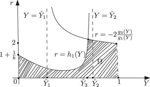
(). Now, we can determine the basin of attraction Ω of (x*, y*), keeping a>1/k fixed, as
Figure 4. Position of Ŷ3(k) for k∈(⅓, 1].
![Figure 4. Position of Ŷ3(k) for k∈(⅓, 1].](/cms/asset/a3227bd9-bd49-4af1-94d2-0ff69ef50a9b/tjbd_a_927596_f0004_b.gif)
The shape of the region Ω in (Y, r)-plane is shown in . It is noted that Elaydi et al. [Citation10] obtain the stability region for positive fixed point in parameter space by using a numerical method.
Figure 5. Shape of Ω in the case k>1.
3.1. Case 0<k≤1
For the functions g1(Y) and g2(Y) defined in Equations (27) and (28), in this case, we have the following properties: for Y<1;
;
;
. This implies that for 0<k≤1 and Y∈(0, 1) the function g1 has no zero, while g2 has a unique zero (). For 0<k≤1, suppose that
be the unique zero of g2(Y) and let Ŷ3(k) be as before, i.e. the unique solution of
where
and the functions h1 and h2 are given by Equations (30) and (31). Then we have
. Therefore, the stability region Ω for the positive fixed point, in this case, is also determined by
Figure 6. Graph of the functions g1 and g2 in the case 0<k≤1.
For a picture of Ω in this case, see .
Figure 7. Shape of Ω in the case 0<k≤1.
It is worth noting that for a given k>0, when one chooses a pair (Y*, r) of Ω, the value of the parameter a>1/k is immediately specified by Equation (23).
Here, the local stability analysis of the fixed points is finished. Now we are in a position that our attention goes to treat bifurcations in the biological model under consideration. This will be done shortly in the next section.
4. Bifurcations of fixed points
In this section, we are planning to do the analysis of the local bifurcations of the fixed points of the system (16), including Neimark–Sacker and period-doubling bifurcations.
4.1. The Neimark–Sacker bifurcation
In the discrete setting, the Neimark–Sacker bifurcation is the analogue of the Hopf bifurcation that occurs in the continuous systems. It was discovered by Neimark [Citation20], and independently by Sacker [Citation22], who originally studied it in (connection) line with the stability of periodic solutions of ordinary differential equations, where it arises from the map obtained by taking a Poincare section transverse to the periodic flow. Hopf bifurcations create limit cycles in the phase plane of continuous models. On the other hand, Neimark–Sacker bifurcations generate dynamically invariant circles. As a result, we may find isolated periodic orbits as well as trajectories that cover the invariant circle densely. We seek conditions for Equation (16) to have a non-hyperbolic fixed point with a pair of complex conjugate eigenvalues of modulus 1. This happens surely at the interior fixed point (x*, y*). The associated Jacobian matrix has two complex conjugate eigenvalues with modulus 1 in the case det(J)=1 and
. Hence, the candidate for the bifurcation curve is the curve
We consider (k, a) as fixed and take r>0 as a parameter and write it as r=r*+μ, where
Following the standard way, we first must do some preliminary (linear or affine) transformations in order to put the linear part of the two-dimensional map (16) into normal form. This will be done shortly. Utilizing the linear transformation
we get the following
two-dimensional map defined by
In the expanded form, we obtain that
Now, the eigenvalues of the linear part of Equation (35) are given by
More precisely, it follows from Equation (35) that
With a linear change of coordinates, we can put the two-dimensional map defined by Equation (34) in the following form:
where
, i=1, 2, are nonlinear in
and
. To simplify the notation, let us define
We make the linear transformation
to obtain the following two-dimensional map defined by
To analyse the corresponding bifurcation, we introduce the complex variables
By Equation (39), the equation for w reads
Now it follows from the normal form theorem for the Neimark–Sacker bifurcation that the one-dimensional map defined by Equation (40) can be transformed by an invertible parameter-dependent change of complex coordinate, which is smoothly dependent on the parameter,
for μ near zero, into a map with only the resonant cubic term:
Remark 4.1 Any such map (39) has the normal form (41) near μ=0 provided that for q=1, 2, 3, 4. Subject to the further condition that
, for sufficiently small μ the map has an invariant closed curve enclosing the origin when
. In the case that
, the bifurcation is said to be supercritical, and there is a stable attracting invariant curve for small enough μ>0, while a subcritical bifurcation arises for
, when there is a repelling invariant curve for small μ<0 (see [Citation18] for more details).
Writing and
, expression (41) can be written as
Remark 4.2 Due to the technical nature of the coefficients (depending on the parameter) appeared for the expressions of N1, N2, D1, D2 in Equation (46) and for the expressions of N, D in Equation (47), we decided to choose some values for the parameters (a, k) and then follow the whole procedure constructed along the paper. By this choice of parameters, we can obtain the exact value of the positive fixed point (x*, y*).
By following computations presented in the paper, we can finally find the value of a(0). For example, if we choose a=10 and k=0.5, then we find that and then
. Thus, for r>r* we have a closed invariant curve which is stable (). On this bases, is constructed by using numerical computations. In order to support the results, phase diagrams for some particular parameter values would be presented for the Neimark–Sacker bifurcation in .
Figure 8. Phase diagram when r=3.7, a=10, k=0.5, (x0, y0)=(0.3, 0.3) and n=25, 000.
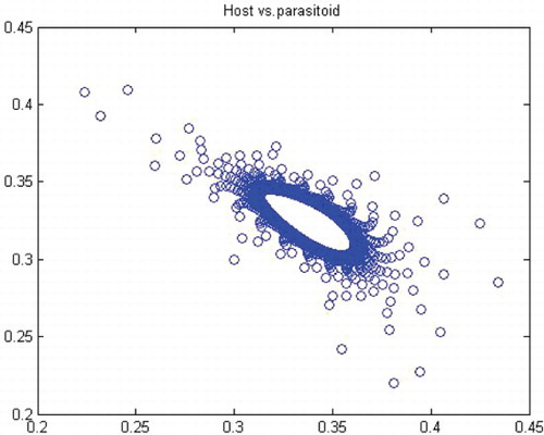
Figure 9. Phase diagram when r=3.6, a=10, k=0.5, (x0, y0)=(0.3, 0.3) and n=25, 000.
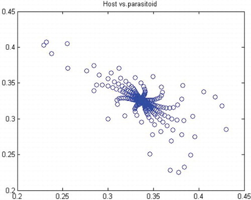
Figure 10. Phase diagram when r=1.6, a=27, k=2, (x0, y0)=(0.6, 0.6) and n=25, 000.
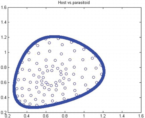
Figure 11. Phase diagram when r=1.49, a=27, k=2, (x0, y0)=(0.6, 0.6) and n=25, 000.
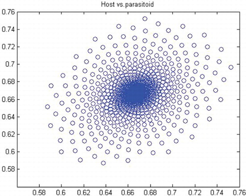
Figure 12. Phase diagram when r=2.2, a=50, k=0.9, (x0, y0)=(0.5, 0.5) and n=25, 000.
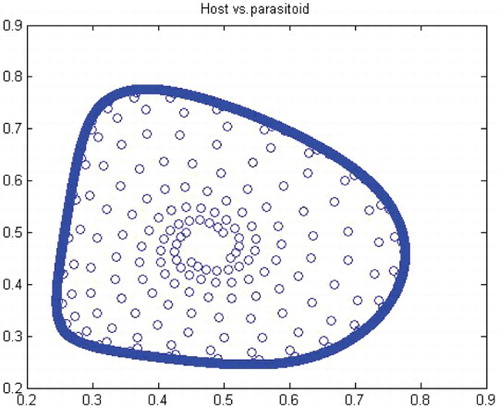
Figure 13. Phase diagram when r=2.0, a=50, k=0.9, (x0, y0)=(0.5, 0.5) and n=25, 000.
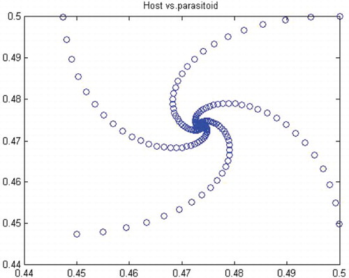
Table 1. The numerical exact values for the positive fixed point (x*, y*) and for the coefficient a(0) corresponding to the chosen values of the parameters (a, k).
4.2. Period-doubling bifurcation
In this subsection, we are planning to do the analysis of the period-doubling bifurcation. In the first step, let k>0 be fixed and consider the function
Then
Moreover,
For k>1 we have E1(Y)>0 when , where Ŷ1 is the unique solution of g1(Y)=0. Clearly the values of Ŷ1 depend on 1<k<∞ adding that
as
,
as
, and Ŷ1=0.5 when k=3.38630. For 0<k≤1 the function E1(Y) is strictly decreasing and positive in the interval (0, 1). When k=1 this function is strictly decreasing from +∞ to +2.
We note that λ=1 is an eigenvalue of the Jacobian matrix J of the system (17) at the fixed point (x*, y*) if and only if which yields r=0. Note that r=0 is not biologically of interest. On the other hand, λ=−1 is an eigenvalue of the Jacobian matrix J of the system (17) at the fixed point (x*, y*) if and only if
which yields r=r1, where
defined by Equation (48). The other eigenvalue of J for r=r1 is given by
, where
We have the following properties of the function E2(Y) defined by Equation (49):
For 0<k<1, the function E2(Y) is strictly increasing on the interval (0, 1) and its values change from 2k/(k−1) to 1 when Y increases. When k>1, let be the unique zero of g1(Y). Then one has for
that
. Now, we treat the dynamics on the centre manifold of the fixed point (x*, y*) in the case r=r1 with
. To do this, we have to place the fixed point at the origin. Let
Then according to Equation (17) and using Equation (37), we get the following two-dimensional map defined by
For we have the eigenvalues
with eigenvectors
Introducing the change of variables
and applying to the previous map, we obtain the following two-dimensional map defined by
Here, we do not give the explicit expressions for the other coefficients of Equation (50), because they are out of use. In fact, the centre manifold will be given as a graph over u and ,
, and be at least O(2). Thus, by computing the centre manifold as
we can immediately see that the reduced map
is given by
A direct calculation yields that
Therefore, the one-dimensional map defined by Equation (51) undergoes a period-doubling bifurcation at
provided that
By an easy computation, we can find that
Remark 4.3 Due to the complicated nature of the expressions (depending on the parameter) in Equations (50)–(52), we decided to choose some particular values for the parameters (a, k) and then follow the whole procedure made along this section. By this choice of parameters, we can determine the exact value of . By following computations presented in this section, we can compute the value of F given by Equation (52). For this reason, is constructed by using numerical computations.
Table 2. The numerical exact values for (r1, λ2, F) corresponding to the chosen parameter values for (a, k).
4.3. Conclusions
In this paper, we studied a discrete-time predator–prey model which was a generalized Beddington–Nicholson–Bailey model. It is also a generalization of the system studied by Hone, Irle and Thurura. We investigated the stability and bifurcations of a generalized Beddington host–parasitoid model. We were able to compute the normal form coefficients of the Neimark–Sacker bifurcation without having the explicit form of the positive fixed point. The coefficients were very long and involved so that we decided to give numerical results along with phase diagrams ( and and ) to verify our findings. The presence of the Neimark–Sacker bifurcation was shown. The same process was done for the period-doubling bifurcation in standard way without knowing the exact value of the positive fixed point. For the positive fixed point, the stability region was obtained in (Y, r)-space. Moreover, the stability condition of the extinction fixed point (0, 0) and the exclusion fixed point (k, 0) was investigated in a standard way. Our system for values b=r=2 and a=1/k seems to have simple dynamics, but it needs further study to obtain the global dynamics. Future research will focus on the global stability of the system and on the study of the other types of bifurcations and dynamics phenomena. This includes a deeper discussion and a further study.
Acknowledgement
This research is supported by Isfahan University of Technology. R.A. thanks Isfahan University of Technology for support.
References
- S. Agarwal and M. Fan, Periodic solutions of non-autonomous discrete predator–prey system of Lotka–Volterra type, Appl. Anal. 81 (2002), pp. 801–812. doi: 10.1080/0003681021000004438
- H.N. Agiza, E. Elabbasy, A.A. Elasdany, and M.H. Metwally, Chaotic dynamics of a discrete prey–predator model with Holling type II, Nonlinear Anal. Real World Appl. 10 (2009), pp. 116–119. doi: 10.1016/j.nonrwa.2007.08.029
- R.M. Anderson, M.P. Hassell, R.M. May, and D.W. Tonkyn, Density dependence in host–parasitoid models, J. Anim. Ecol. 50 (1981), pp. 855–865. doi: 10.2307/4080
- D. Armbruster, Y. Kang, and Y. Kuang, Dynamics of a plant–herbivore model, J. Biol. Dyn. 2 (2008), pp. 89–101. doi: 10.1080/17513750801956313
- V.A. Bailey and A.J. Nicholson, The balance of animal populations, I Proc. Zool. Soc. Lond. 3 (1935), pp. 551–598.
- J.R. Beddington, C.A. Free, and J.H. Lawton, Dynamic complexity in predator–prey models framed in difference equations, Nature 225 (1975), pp. 58–60. doi: 10.1038/255058a0
- H. Brian, C. Justian, and D. Summers, Chaos in periodically forced discrete-time ecosystem models, Chaos Solitons Fractals 11 (2000), pp. 2331–2342. doi: 10.1016/S0960-0779(99)00154-X
- B.D. Corbett, and S.M. Moghadas, Limit cycles in a generalized Gause-type predator–prey model, Chaos Solitons Fractals 37 (2008), pp. 1343–1355. doi: 10.1016/j.chaos.2006.10.017
- L. Edelstein-Keshet, Mathematical Models in Biology, SIAM, Philadelphia, PA, 2005.
- S. Elaydi, S. Kapçak, and U. Ufuktepe, Stability and invariant manifolds of a generalized Beddington host–parasitoid model, J. Biol. Dyn. 7(1) (2013), pp. 233–253. doi: 10.1080/17513758.2013.849764
- M. Fan and K. Wang, Periodic solutions of a discrete time nonautonomous ratio-dependent predator–prey system, Math. Comput. Model. 35 (2002), pp. 951–961. doi: 10.1016/S0895-7177(02)00062-6
- A.N. Hone, M.V. Irle, and G.W. Thurura, On the Neimark–Sacker bifurcation in a discrete predator–prey system, J. Biol. Dyn. 4(6) (2010), pp. 594–606. doi: 10.1080/17513750903528192
- H.F. Huo and W.T. Li, Existence and global stability of periodic solutions of a discrete predator–prey system with delays, Appl. Math. Comput. 153 (2004), pp. 337–351. doi: 10.1016/S0096-3003(03)00635-0
- G. Jiang and Q. Lu, Impulsive state feedback of a predator–prey model, J. Comput. Appl. Math. 200 (2007), pp. 193–207. doi: 10.1016/j.cam.2005.12.013
- G. Jiang, Q. Lu, and L. Qian, Complex dynamics of a Holling type II prey–predator system with state feedback control, Chaos Solitons Fractals 31 (2007), pp. 448–461. doi: 10.1016/j.chaos.2005.09.077
- Z. Jing and J. Yang, Bifurcation and chaos in discrete time predatorprey system, Chaos Solitons Fractals 27 (2000), pp. 259–277. doi: 10.1016/j.chaos.2005.03.040
- B.E. Kendall, Cycles, Chaos and noise in predator–prey dynamics, Chaos Solitons Fractals 12 (2001), pp. 321–332. doi: 10.1016/S0960-0779(00)00180-6
- Y. Kuznetsov, Elements of Applied Bifurcation Theory, Springer, New York, 1998.
- X. Liu and D. Xiao, Complex dynamic behaviour of a discrete time predator–prey system, Chaos Solitons Fractals 32 (2007), pp. 80–94. doi: 10.1016/j.chaos.2005.10.081
- Y. Neimark, On some cases of periodic motions depending on parameters, Dokl. Acad. Nauk. SSSR 129 (1959), pp. 736–739.
- W.E. Ricker, Stock and recruitment, J. Fish. Res. Board Can. 11 (1954), pp. 559–623. doi: 10.1139/f54-039
- R.J. Sacker, On invariant surfaces and bifurcation of periodic solutions of ordinary differential equations, Ph.D. thesis, IMM-NYU 333, Courant Institute, New York University, 1964.