A new approach for designing disease intervention strategies in metapopulation models

ABSTRACT

We describe a new approach for investigating the control strategies of compartmental disease transmission models. The method rests on the construction of various alternative next-generation matrices, and makes use of the type reproduction number and the target reproduction number. A general metapopulation SIRS (susceptible–infected–recovered–susceptible) model is given to illustrate the application of the method. Such model is useful to study a wide variety of diseases where the population is distributed over geographically separated regions. Considering various control measures such as vaccination, social distancing, and travel restrictions, the procedure allows us to precisely describe in terms of the model parameters, how control methods should be implemented in the SIRS model to ensure disease elimination. In particular, we characterize cases where changing only the travel rates between the regions is sufficient to prevent an outbreak.

KEYWORDS:

• Metapopulation epidemic models
• intervention strategies
• type reproduction number
• target reproduction number
• alternative next-generation matrix

AMS SUBJECT CLASSIFICATION:

• 92D30

1. Introduction

In mathematical epidemiology, one of the most important issues is to determine whether an infectious disease can invade a susceptible population. The basic reproduction number (${\mathcal{R}}_0$), defined as the expected number of secondary cases generated by a typical infected host introduced into a susceptible population [1, 7, 17], serves as a threshold quantity for epidemic outbreaks. The next-generation matrix (NGM), initially introduced by Diekmann et al. [7], provides a powerful approach to derive the basic reproduction number. This matrix (often denoted by $\mathbf{K}\mathbf{=}\mathbf{\left[}{\mathbf{k}}_{\mathbf{i}\mathbf{j}}\mathbf{\right]}$) gives the average number of new infections among the susceptible individuals of type i, generated by an infected individual of type j. The NGM is nonnegative, and ${\mathcal{R}}_0$ is identified as its dominant eigenvalue, that is, ${\mathcal{R}}_0=\rho \left(\mathbf{K}\mathbf{\right)}$.

If ${\mathcal{R}}_0>1$ then the disease can persist in the population. For successful disease elimination, it is necessary to decrease ${\mathcal{R}}_0$ below 1, that may be achieved by implementing intervention strategies. Vaccination targets particular or all individual groups, and decreases the fraction of the population susceptible to the disease, thereby reducing the reproduction number. Another powerful tool in endemic situations is to decrease the probability of transmission, by reducing the interaction between particular groups within the population, or by reducing the contact between infected and susceptible individuals.

When modelling the prevention and control strategies of infectious diseases, the goal is to bring ${\mathcal{R}}_0$ below 1 by controlling various model parameters. However, in many models the reproduction number is often obtained as a complicated expression of the parameters, and it may be difficult to determine how the parameters should be changed to decrease ${\mathcal{R}}_0$. Entries of the NGM usually arise by less complicated formulas than that one of the reproduction number. Assume that by controlling model parameters, for each entry of the NGM a proportion more than $1-1/{\mathcal{R}}_0$ of the entry is reduced. Then it follows from the definition ${\mathcal{R}}_0=\rho \left(\mathbf{K}\mathbf{\right)}$ (where $\mathbf{K}$ is the NGM) that the dominant eigenvalue of the NGM drops below 1 and the outbreak is prevented. Not only is the basic reproduction number a threshold for epidemic outbreaks, but it also determines the critical effort needed to eliminate infection from the population, provided that all entries of the NGM can be controlled.

In some situations, however, there are limitations in implementing intervention strategies, so there may be some entries of the NGM that are not subject to change. This was noted by Heesterbeek and Roberts [10], Roberts and Heesterbeek [13], and Shuai et al. [15], who developed methods to decrease ${\mathcal{R}}_0$ by reducing only particular elements of the NGM. The procedure of Heesterbeek and Roberts [10] and Roberts and Heesterbeek [13] applies to entire columns or rows of the NGM, and is based on the consideration that control is often aimed at only particular disease compartments, such as specific host types in multi-host models (e.g. vector control) or a particular group of individuals in heterogeneous population models. Shuai et al. [15] extend the ideas of the above works, and address the cases where control targets the interactions between different types of individuals. The method of Shuai et al. [15] reduces individual entries of the NGM, or sets of such entries. In both approaches mentioned above, new quantities are introduced – the type reproduction number in [10,13] and the target reproduction number in [15] – that measure the strength of the effort needed to prevent outbreaks. However, when applied to specific disease transmission models, these procedures do not characterize in terms of the model parameters, how the intervention should be executed. In fact, control strategies are often aimed at particular model parameters rather than entries of the NGM.

In this paper, we address the gap in previous works, and present an approach for the design of control strategies that determines how model parameters should be changed to prevent outbreaks. Our procedure rests on various ‘alternative’ next-generation matrices that one can define for a disease transmission model. Applying this method, we systematically investigate the intervention strategies of a general SIRS (susceptible–infected–recovered–susceptible) model, that is appropriate for the spread of an infectious disease in a geographically dispersed metapopulation of individuals. While the qualitative properties of metapopulation (patchy) epidemic models have been widely studied in the literature, evaluating the intervention strategies in these models has received less attention (see, for instance, [2, 3, 6, 11, 14, 18, 19] and the references therein). It is particularly challenging to understand the dependence of movement between populations on the reproduction number [2, 4,5]. Our procedure allows for the design of intervention strategies that target exclusively the movement of particular groups in the metapopulation SIRS model. Making use of the methods proposed in [10, 13, 15], we identify controllable model parameters, and characterize various control strategies in terms of the targeted parameters. The procedure of how these parameters should be changed to execute control will be precisely described. We give conditions for cases where changing movement rates exclusively is sufficient for disease elimination, and provide recommendation for intervention in both local (patch-wise) and global scale.

The paper is organized as follows. After describing our approach in Section 2, we demonstrate the use of the method on a two-patch SIRS model in Section 3, where feasible control approaches will be systematically investigated. Section 4 is devoted to the intervention strategies of a more general metapopulation SIRS model in r patches. Finally, we discuss our findings in the last section.

2. Description of the method

First, we recall the main steps of the procedure described by Diekmann et al. [8], for the calculation of the basic reproduction number in compartmental epidemic models. For this approach, the population of infected individuals is divided into discrete categories, and one needs to derive the average number of secondary cases per one infected individual in the various categories, in the initial phase of the epidemic. This way, the NGM is constructed (denoted by $\mathbf{K}$), and ${\mathcal{R}}_0$ is identified as the dominant eigenvalue of the NGM, that is, ${\mathcal{R}}_0=\rho \left(\mathbf{K}\mathbf{\right)}$.

To derive the NGM, one identifies the infection subsystem in the compartmental model, that is, the equations that describe the generation of new infections and changes in the epidemiological statuses among infected individuals. The matrix of the linearization of the infection subsystem about the disease-free equilibrium (DFE) gives the Jacobian $\mathbf{J}$. Then, $\mathbf{J}$ is decomposed as $\mathbf{F}\mathbf{-}\mathbf{V}$, where $\mathbf{F}$ describes the production of new infections (transmission part in the linear approximation), and $\mathbf{V}$ represents changes in status, as recovery or death (transition part in the linear approximation). Under the conditions that are satisfied in epidemic models, the inverse of $\mathbf{V}$ exists and ${\mathbf{V}}^{\mathbf{-}\mathbf{1}}\ge \mathbf{0}$, and the product of $\mathbf{F}$ and ${\mathbf{V}}^{\mathbf{-}\mathbf{1}}$ gives ‘the NGM with Large domain’ (see [8]). In some cases (e.g. for SLIR-based models with latent period), further steps are required to obtain $\mathbf{K}$ (the NGM) from $\mathbf{F}\cdot {\mathbf{V}}^{\mathbf{-}\mathbf{1}}$, since the decomposition relates the expected offspring of individuals of any status (both latent and infected statuses in the SLIR model) and not just new infections. However, these matrices have the same spectral radii, that is, $\rho \left(\mathbf{K}\mathbf{\right)}\mathbf{=}\rho \mathbf{(}\mathbf{F}\cdot {\mathbf{V}}^{\mathbf{-}\mathbf{1}}\mathbf{)}$. In SIR- and SIRS-type models, it holds that $\mathbf{F}\cdot {\mathbf{V}}^{\mathbf{-}\mathbf{1}}\mathbf{=}\mathbf{K}$. Nevertheless, it is meaningful to define ${\mathcal{R}}_0$ as ${\mathcal{R}}_0=\rho (\mathbf{F}\cdot {\mathbf{V}}^{\mathbf{-}\mathbf{1}}\mathbf{)}$ [8].

The criterion saying that the disease can invade into the population if ${\mathcal{R}}_0>1$ whereas it cannot if ${\mathcal{R}}_0<1$, follows from the result that the dominant eigenvalue (the spectral radius) of $\mathbf{F}\cdot {\mathbf{V}}^{\mathbf{-}\mathbf{1}}$ gives a threshold for the stability of the DFE [8]. This result is shown in terms of M-matrices by van den Driessche and Watmough [17]. We say that a square matrix $\mathbf{A}$ has the Z-sign pattern if all entries of $\mathbf{A}$ are non-positive except possibly those in the diagonal. If $\mathbf{A}$ has the Z-sign pattern and ${\mathbf{A}}^{\mathbf{-}\mathbf{1}}\ge \mathbf{0}$ holds then we say that $\mathbf{A}$ is a non-singular M-matrix (several definitions exist for M-matrices, see [9, Theorem 5.1]). In the vast majority of epidemic models – including the ones considered in this paper – these conditions are satisfied for the matrix $\mathbf{V}$. By the definition of $\mathbf{F}$, it also holds that $\mathbf{F}$ is a nonnegative matrix.

Now, we discuss how to construct ‘alternative’ next-generation matrices. Besides the matrices $\mathbf{F}$ for new infections and $\mathbf{V}$ for transfer between classes, there may exist different splittings of the Jacobian that satisfy the same conditions as $\mathbf{F}$ and $\mathbf{V}$. Consider matrices $\tilde{\mathbf{V}}$ and $\tilde{\mathbf{V}}$ such that $\mathbf{J}\mathbf{=}\stackrel{\mathbf{~}}{\mathbf{F}}\mathbf{-}\stackrel{\mathbf{~}}{\mathbf{V}}$, $\tilde{\mathbf{V}}$ is a nonnegative matrix and $\tilde{\mathbf{V}}$ is a non-singular M-matrix. Then, the matrix $\tilde{\mathbf{K}}$, defined by $\tilde{\mathbf{K}}:=\tilde{\mathbf{F}}\cdot {\tilde{\mathbf{V}}}^{-1}$, serves as an alternative NGM. Albeit the NGM is not necessarily irreducible, here we only consider splittings such that $\tilde{\mathbf{K}}$ is irreducible. As $\tilde{\mathbf{V}}$ and $\tilde{\mathbf{V}}$ have the same properties as $\mathbf{F}$ and $\mathbf{V}$, respectively, it follows that $\rho (\tilde{\mathbf{F}}\cdot {\tilde{\mathbf{V}}}^{-1})$ and $\rho (\mathbf{F}\cdot {\mathbf{V}}^{\mathbf{-}\mathbf{1}}\mathbf{)}$ agree at the threshold value 1. In fact, we can say more:

Proposition 2.1:

Consider a splitting $\tilde{\mathbf{F}}-\tilde{\mathbf{V}}$ of the Jacobian of the infected subsystem about the DFE, where $\tilde{\mathbf{V}}$ is a nonnegative matrix and $\tilde{\mathbf{V}}$ is a non-singular M-matrix. Then for the matrix $\tilde{\mathbf{K}}=\tilde{\mathbf{F}}\cdot {\tilde{\mathbf{V}}}^{-1},$ it holds that ${\mathcal{R}}_0<1$ if and only if $\rho \left(\tilde{\mathbf{K}}\right)<1,$ ${\mathcal{R}}_0=1$ if and only if $\rho \left(\tilde{\mathbf{K}}\right)=1,$ and ${\mathcal{R}}_0>1$ if and only if $\rho \left(\tilde{\mathbf{K}}\right)>1$.

Proof:

By similar arguments as in the proof of Theorem 2 in [17], we claim that $s\left(\mathbf{J}\right)<0$ if and only if $\rho (\tilde{\mathbf{F}}\cdot {\tilde{\mathbf{V}}}^{-1})<1$, $s\left(\mathbf{J}\right)=0$ if and only if $\rho (\tilde{\mathbf{F}}\cdot {\tilde{\mathbf{V}}}^{-1})=1$, and $s\left(\mathbf{J}\right)>0$ if and only if $\rho (\tilde{\mathbf{F}}\cdot {\tilde{\mathbf{V}}}^{-1})>1$, where $s\left(\mathbf{J}\right)$ denotes the maximum real part of all eigenvalues of $\mathbf{J}$. Note that this statement holds true for any $\tilde{\mathbf{V}}$ and $\tilde{\mathbf{V}}$ that satisfy the conditions of the proposition. The matrix for new infections $\mathbf{F}$, and $\mathbf{V}$ for the transitions between infected statuses, give special cases of such $\tilde{\mathbf{V}}$ and $\tilde{\mathbf{V}}$, respectively. We remind that ${\mathcal{R}}_0=\rho (\mathbf{F}\cdot {\mathbf{V}}^{-1})$ and $\tilde{\mathbf{K}}=\tilde{\mathbf{F}}\cdot {\tilde{\mathbf{V}}}^{-1}$, that complete the proof.

Next, we give a brief overview of how the methods of Heesterbeek and Roberts [10, 13], and Shuai et al. [15] (see also [16] for Erratum) work on the NGM. We follow the terminology of the latter as it generalizes the former. For the NGM $\mathbf{K}\mathbf{=}\mathbf{\left[}{\mathbf{k}}_{\mathbf{i}\mathbf{j}}\mathbf{\right]}$, one identifies the set of targeted entries S, that is, the set of entries in $\mathbf{K}$ that are subject to change in control. The target matrix ${\mathbf{K}}_{\mathbf{S}}$ is identified as $[{\mathbf{K}}_{\mathbf{S}}{\mathbf{]}}_{\mathbf{i}\mathbf{j}}\mathbf{=}{\mathbf{k}}_{\mathbf{i}\mathbf{j}}$ if $(i,j)\in S$, and zero otherwise. The target reproduction number ${\mathcal{T}}_S$ is defined as ${\mathcal{T}}_S=\rho ({\mathbf{K}}_{\mathbf{S}}\cdot \mathbf{(}\mathbf{I}\mathbf{-}\mathbf{K}\mathbf{+}{\mathbf{K}}_{\mathbf{S}}{\mathbf{)}}^{\mathbf{-}\mathbf{1}}\mathbf{)}$ provided that $\rho (\mathbf{K}\mathbf{-}{\mathbf{K}}_{\mathbf{S}}\mathbf{)}\mathbf{<}\mathbf{1}$, where $\mathbf{I}$ is the identity matrix. The last condition can be referred to as the condition for controllability, since if the spectral radius is greater than 1 then the disease cannot be eliminated by targeting only S (in such case, ${\mathcal{T}}_S$ is not defined [15]). The controlled NGM ${\mathbf{K}}_{\mathbf{c}}$ is formulated by replacing the entry $k_{ij}$ in $\mathbf{K}$ by $k_{ij}/{\mathcal{T}}_S$ whenever $(i,j)\in S$.

Theorem 2.1 in [15] states that if $\mathbf{K}$ is irreducible and the condition for controllability holds, then ${\mathcal{T}}_S>1$ if and only if ${\mathcal{R}}_0>1$. According to Shuai et al. [15, Theorem 2.2], the controlled next-generation matrix satisfies $\rho \left({\mathbf{K}}_{\mathbf{c}}\mathbf{\right)}\mathbf{=}\mathbf{1}$. Similar to the basic reproduction number, the target reproduction number ${\mathcal{T}}_S$ serves as a quantity to measure the effort needed to eliminate the disease, when control is applied on the set S.

Now, we are ready to describe a procedure that will allow us to design and systematically investigate the intervention strategies of compartmental epidemic models. Assume that ${\mathcal{R}}_0>1$ and the disease can invade the population; otherwise no control is necessary. First, we identify a set of model parameters $\mathrm{\Omega }=({\omega }_1,\dots ,{\omega }_n)$ that are subject to change in the control. Then, we decompose the Jacobian of the infected subsystem as $\mathbf{J}\mathbf{=}\stackrel{\mathbf{~}}{\mathbf{F}}\mathbf{-}\stackrel{\mathbf{~}}{\mathbf{V}}$, to construct an alternative NGM $\tilde{\mathbf{K}}:=\tilde{\mathbf{F}}\cdot {\tilde{\mathbf{V}}}^{-1}.$ $\tilde{\mathbf{V}}$ and $\tilde{\mathbf{V}}$ in the decomposition must satisfy the conditions of Proposition 2.1, moreover we only consider splittings such that $\tilde{\mathbf{K}}$ is irreducible. Next, we select the entries of $\tilde{\mathbf{K}}=\left[{\tilde{k}}_{ij}\right]$ that depend on the parameters in Ω, and define the target set $\tilde{S}$ as the set of the indices of the entries. With $\tilde{S}=\left(\right(i_1,j_1),\dots ,(i_m,j_m\left)\right),$ the entry ${\tilde{k}}_{ij}$ depends on some of the parameters ${\omega }_1,\dots ,{\omega }_n$ for $(i,j)=(i_1,j_1),\dots ,$ $(i_m,j_m)$, and otherwise ${\tilde{k}}_{ij}$ is independent of each parameter in Ω. Given $\tilde{S}$, we follow the description above to construct the target matrix ${\tilde{\mathbf{K}}}_{\tilde{\mathbf{S}}}$ as $[{\tilde{\mathbf{K}}}_{\tilde{\mathbf{S}}}{]}_{ij}:=\left\{\begin{array}{ll}{\tilde{k}}_{ij}& \mathrm{if}(i,j)\in \tilde{S},\\ 0& \mathrm{otherwise},\end{array}\right.$ and obtain the controllability condition $\rho (\tilde{\mathbf{K}}-{\tilde{\mathbf{K}}}_{\tilde{\mathbf{S}}})<1.$ Provided that the controllability condition holds, the target reproduction number is defined as ${\mathcal{T}}_{\tilde{S}}:=\rho ({\tilde{\mathbf{K}}}_{\tilde{\mathbf{S}}}\cdot (\mathbf{I}\mathbf{-}\stackrel{\mathbf{~}}{\mathbf{K}}\mathbf{+}{\stackrel{\mathbf{~}}{\mathbf{K}}}_{\stackrel{\mathbf{~}}{\mathbf{S}}}{\mathbf{)}}^{\mathbf{-}\mathbf{1}}\mathbf{)}\mathbf{,}$ and the controlled alternative NGM ${\tilde{\mathbf{K}}}_{\mathbf{c}}$ is formulated as $\begin{array}{r}[{\tilde{\mathbf{K}}}_{\mathbf{c}}{]}_{ij}:=\left\{\begin{array}{ll}\frac{{\tilde{k}}_{ij}}{{\mathcal{T}}_{\tilde{S}}}& \mathrm{if}(i,j)\in \tilde{S},\\ {\tilde{k}}_{ij}& \mathrm{otherwise}.\end{array}\right.\end{array}$

The assumption that ${\mathcal{R}}_0>1$, implies by [15, Theorem 2.1] that ${\mathcal{T}}_{\tilde{S}}>1$. The goal is to reduce the proportion $1-1/{\mathcal{T}}_{\tilde{S}}$ of all entries in $\tilde{S}$, since this way $\tilde{\mathbf{K}}$ is transformed into ${\tilde{\mathbf{K}}}_{\mathbf{c}}$ and $\rho \left({\tilde{\mathbf{K}}}_{\mathbf{c}}\right)=1$ implies that the disease can be eradicated (see [15, Theorem 2.2]). Thus, our last step is to characterize how each targeted parameter ${\omega }_1,\dots ,{\omega }_n$ should be changed such that $\tilde{\mathbf{K}}$ is transformed into ${\tilde{\mathbf{K}}}_{\mathbf{c}}$. To formalize this, we think of $\tilde{\mathbf{K}}=\tilde{\mathbf{K}}\left(\mathrm{\Omega }\right)$ as a matrix that is dependent of the targeted parameters, and look for ${\mathrm{\Omega }}_c=({\omega }_1^c,\dots ,{\omega }_n^c)$ such that $\tilde{\mathbf{K}}\left({\mathrm{\Omega }}_c\right)={\tilde{\mathbf{K}}}_{\mathbf{c}}$ holds, where ${\mathrm{\Omega }}_c$ is the set of targeted parameters after control. To this end, the functions ${\phi }_1,\dots ,{\phi }_n$ need to be identified that transform targeted parameters such that ${\phi }_1\left({\omega }_1\right)={\omega }_1^c,\dots ,{\phi }_n\left({\omega }_n\right)={\omega }_n^c.$

Different control approaches (that is, different choices of the set of targeted parameters) may require the construction of different alternative next-generation matrices. We will see in the analysis of the proposed models that some splittings of the Jacobian are easier to handle than others. Each alternative NGM provides an alternative threshold quantity for disease elimination (see Proposition 2.1); this number, however, is not equal to the basic reproduction number. Hence, the significance of this alternative threshold quantity is that reducing it to 1 by means of epidemic control ensures disease elimination, but this number is not useful for estimating ${\mathcal{R}}_0$.

The above-described procedure readily allows us to compare control approaches, by means of their properties as the controllability condition and the target reproduction number. We will give examples when the controllability condition (a condition of the model parameters) holds for one control strategy but cannot be satisfied for another. By the transformation of targeted parameters that ensures disease eradication, we can determine the critical control effort needed to prevent an outbreak. Doing so for each feasible intervention strategy, we become capable of evaluating the advantages of one over another. Hence, the analysis is applicable to provide recommendation, when it comes to making decisions about which control strategy is best to implement.

3. Control in a two-patch SIRS model

We consider the classical SIRS model in two patches that are connected by individuals' travel. In patch i ($i\in \{1,2\}$), we denote the total population at time t by $N_i\left(t\right)$, whereas $S_i\left(t\right)$, $I_i\left(t\right)$, and $R_i\left(t\right)$ give the numbers of susceptible, infected, and recovered individuals, respectively, at time t. It holds for any $t\ge 0$ that $S_i\left(t\right)+I_i\left(t\right)+R_i\left(t\right)=N_i\left(t\right)$. Recruitment into the susceptible class of patch i is described by ${\mathrm{\Lambda }}_i\left(N_i\right)$, and $d_i$ is the constant death rate. Disease transmission in patch i is modelled by the term ${\beta }_i{S}_i\left(t\right)I_i\left(t\right)/N_i\left(t\right)$ (standard incidence), where ${\beta }_i$ is the constant transmission rate. We denote by ${\alpha }_i$ the recovery rate of infected individuals, and ${\theta }_i$ is the rate of losing immunity. Note that if ${\theta }_i=0$ then the model in patch i reduces to the classical SIR model, whereas with ${\theta }_i\to \mathrm{\infty }$ it is assumed that the period of immunity is so short that it can be ignored, and we arrive at a model equivalent to the SIS model. To incorporate movements between the patches, we introduce the parameters $m_{12}$ and $m_{21}$ for the travel rate from patch 2 to 1, and from patch 1 to 2, respectively. Based on the above assumptions, we give the following system of ODEs to describe the spread of an infectious disease in and between two patches: (M1) $\begin{array}{rl}{S}_1^{\prime }& ={\mathrm{\Lambda }}_1\left(N_1\right)-{\beta }_1\frac{S_1{I}_1}{N_1}-d_1{S}_1+{\theta }_1{R}_1-m_{21}{S}_1+m_{12}{S}_2,\\ I_1^{\prime }& ={\beta }_1\frac{S_1{I}_1}{N_1}-({\alpha }_1+d_1)I_1-m_{21}{I}_1+m_{12}{I}_2,\\ R_1^{\prime }& ={\alpha }_1{I}_1-({\theta }_1+d_1)R_1-m_{21}{R}_1+m_{12}{R}_2,\\ S_2^{\prime }& ={\mathrm{\Lambda }}_2\left(N_2\right)-{\beta }_2\frac{S_2{I}_2}{N_2}-d_2{S}_2+{\theta }_2{R}_2-m_{12}{S}_2+m_{21}{S}_1,\\ I_2^{\prime }& ={\beta }_2\frac{S_2{I}_2}{N_2}-({\alpha }_2+d_2)I_2-m_{12}{I}_2+m_{21}{I}_1,\\ R_1^{\prime }& ={\alpha }_2{I}_2-({\theta }_2+d_2)R_2-m_{12}{R}_2+m_{21}{R}_1.\end{array}$(M1) For the dynamics of the total population in patch 1 and patch 2, we obtain the system $\begin{array}{rl}{N}_1^{\prime }& ={\mathrm{\Lambda }}_1\left(N_1\right)-d_1{N}_1-m_{21}{N}_1+m_{12}{N}_2,\\ N_2^{\prime }& ={\mathrm{\Lambda }}_2\left(N_2\right)-d_2{N}_2-m_{12}{N}_2+m_{21}{N}_1,\end{array}$ for which we assume that there exists a unique equilibrium $({\overline{N}}_1,{\overline{N}}_2)$ (if, for instance, ${\mathrm{\Lambda }}_i\left(N_i\right)=d_i{N}_1$, or if the recruitment is constant, then this assumption is fulfilled). It is easy to see that $({\overline{N}}_1,0,0,{\overline{N}}_2,0,0)$ gives the unique DFE of the system (1(M1) $\begin{array}{rl}{S}_1^{\prime }& ={\mathrm{\Lambda }}_1\left(N_1\right)-{\beta }_1\frac{S_1{I}_1}{N_1}-d_1{S}_1+{\theta }_1{R}_1-m_{21}{S}_1+m_{12}{S}_2,\\ I_1^{\prime }& ={\beta }_1\frac{S_1{I}_1}{N_1}-({\alpha }_1+d_1)I_1-m_{21}{I}_1+m_{12}{I}_2,\\ R_1^{\prime }& ={\alpha }_1{I}_1-({\theta }_1+d_1)R_1-m_{21}{R}_1+m_{12}{R}_2,\\ S_2^{\prime }& ={\mathrm{\Lambda }}_2\left(N_2\right)-{\beta }_2\frac{S_2{I}_2}{N_2}-d_2{S}_2+{\theta }_2{R}_2-m_{12}{S}_2+m_{21}{S}_1,\\ I_2^{\prime }& ={\beta }_2\frac{S_2{I}_2}{N_2}-({\alpha }_2+d_2)I_2-m_{12}{I}_2+m_{21}{I}_1,\\ R_1^{\prime }& ={\alpha }_2{I}_2-({\theta }_2+d_2)R_2-m_{12}{R}_2+m_{21}{R}_1.\end{array}$(M1) ).

We let ${\gamma }_i={\alpha }_i+d_i$, and define the local reproduction number in patch i ($i\in \{1,2\}$) as ${\mathcal{R}}_i=\frac{{\beta }_i}{{\gamma }_i},$ that gives a threshold for the stability of the DFE $({\overline{N}}_i,0,0)$ in the absence of travelling. In the SIRS model (1(M1) $\begin{array}{rl}{S}_1^{\prime }& ={\mathrm{\Lambda }}_1\left(N_1\right)-{\beta }_1\frac{S_1{I}_1}{N_1}-d_1{S}_1+{\theta }_1{R}_1-m_{21}{S}_1+m_{12}{S}_2,\\ I_1^{\prime }& ={\beta }_1\frac{S_1{I}_1}{N_1}-({\alpha }_1+d_1)I_1-m_{21}{I}_1+m_{12}{I}_2,\\ R_1^{\prime }& ={\alpha }_1{I}_1-({\theta }_1+d_1)R_1-m_{21}{R}_1+m_{12}{R}_2,\\ S_2^{\prime }& ={\mathrm{\Lambda }}_2\left(N_2\right)-{\beta }_2\frac{S_2{I}_2}{N_2}-d_2{S}_2+{\theta }_2{R}_2-m_{12}{S}_2+m_{21}{S}_1,\\ I_2^{\prime }& ={\beta }_2\frac{S_2{I}_2}{N_2}-({\alpha }_2+d_2)I_2-m_{12}{I}_2+m_{21}{I}_1,\\ R_1^{\prime }& ={\alpha }_2{I}_2-({\theta }_2+d_2)R_2-m_{12}{R}_2+m_{21}{R}_1.\end{array}$(M1) ), the infected subsystem reads $\begin{array}{rl}{I}_1^{\prime }& ={\beta }_1\frac{S_1{I}_1}{N_1}-{\gamma }_1{I}_1-m_{21}{I}_1+m_{12}{I}_2,\\ I_2^{\prime }& ={\beta }_2\frac{S_2{I}_2}{N_2}-{\gamma }_2{I}_2-m_{12}{I}_2+m_{21}{I}_1,\end{array}$ which we linearize at the DFE to give the $2\times 2$ Jacobian matrix $\mathbf{J}\mathbf{=}\left(\begin{array}{cc}{\beta }_{\mathbf{1}}\mathbf{-}{\gamma }_{\mathbf{1}}\mathbf{-}{\mathbf{m}}_{\mathbf{21}}& m_{12}\\ m_{21}& {\beta }_2-{\gamma }_2-m_{12}\end{array}\right)\mathbf{.}$ To calculate the NGM, we decompose $\mathbf{J}$ into $\mathbf{F}\mathbf{-}\mathbf{V}$, with $\mathbf{F}\mathbf{=}\left(\begin{array}{cc}{\beta }_{\mathbf{1}}& 0\\ 0& {\beta }_2\end{array}\right)\mathbf{,}\mathbf{V}\mathbf{=}\left(\begin{array}{cc}{\gamma }_{\mathbf{1}}\mathbf{+}{\mathbf{m}}_{\mathbf{21}}& -m_{12}\\ -m_{21}& {\gamma }_2+m_{12}\end{array}\right)\mathbf{,}$ to separate new infections from transitions between disease classes in the linear approximation. The matrix $\mathbf{F}$ is nonnegative, and $\mathbf{V}$ has the Z-sign pattern and a nonnegative inverse ($\mathbf{V}$ is a non-singular M-matrix). We derive the NGM $\begin{array}{r}\mathbf{K}\mathbf{=}\mathbf{F}\cdot {\mathbf{V}}^{\mathbf{-}\mathbf{1}}\mathbf{=}\left(\begin{array}{cc}\frac{{\beta }_{\mathbf{1}}\mathbf{(}{\gamma }_{\mathbf{2}}\mathbf{+}{\mathbf{m}}_{\mathbf{12}}\mathbf{)}}{\mathbf{(}{\gamma }_{\mathbf{1}}\mathbf{+}{\mathbf{m}}_{\mathbf{21}}\mathbf{)}\mathbf{(}{\gamma }_{\mathbf{2}}\mathbf{+}{\mathbf{m}}_{\mathbf{12}}\mathbf{)}\mathbf{-}{\mathbf{m}}_{\mathbf{12}}{\mathbf{m}}_{\mathbf{21}}}& \frac{{\beta }_1{m}_{12}}{({\gamma }_1+m_{21})({\gamma }_2+m_{12})-m_{12}{m}_{21}}\\ \frac{{\beta }_2{m}_{21}}{({\gamma }_1+m_{21})({\gamma }_2+m_{12})-m_{12}{m}_{21}}& \frac{{\beta }_2({\gamma }_1+m_{21})}{({\gamma }_1+m_{21})({\gamma }_2+m_{12})-m_{12}{m}_{21}}\end{array}\right)\mathbf{,}\end{array}$ and the basic reproduction number $\begin{array}{rl}{\mathcal{R}}_0& =\rho (\mathbf{F}\cdot {\mathbf{V}}^{\mathbf{-}\mathbf{1}}\mathbf{)}\\ & =\frac{1}{2}\left(\frac{{\beta }_1({\gamma }_2+m_{12})+{\beta }_2({\gamma }_1+m_{21})}{({\gamma }_1+m_{21})({\gamma }_2+m_{12})-m_{12}{m}_{21}}\right.\\ & \left.+\sqrt{{\left(\frac{{\beta }_1({\gamma }_2+m_{12})-{\beta }_2({\gamma }_1+m_{21})}{({\gamma }_1+m_{21})({\gamma }_2+m_{12})-m_{12}{m}_{21}}\right)}^2+\frac{4{\beta }_1{m}_{12}{\beta }_2{m}_{21}}{\left(\right({\gamma }_1+m_{21}\left)\right({\gamma }_2+m_{12})-m_{12}{m}_{21}{)}^2}}\right).\end{array}$

Assuming that ${\mathcal{R}}_0>1$ implying that the disease can invade into the population, potential control strategies may target transmission rates (${\beta }_1$, ${\beta }_2$), travel rates ($m_{12}$, $m_{21}$), or a combination of those above. It is easy to see that decreasing both ${\beta }_1$ and ${\beta }_2$ will decrease all elements of $\mathbf{K}$, and hence ${\mathcal{R}}_0$ as well. However, it is difficult to tell from the formulas of ${\mathcal{R}}_0$ and $\mathbf{K}$ if controlling travel rates can contribute to disease elimination. To answer the above question, it is more convenient to decompose the Jacobian in a way different from $\mathbf{F}\mathbf{-}\mathbf{V}$. With the splitting $\mathbf{J}\mathbf{=}\stackrel{\mathbf{~}}{\mathbf{F}}\mathbf{-}\stackrel{\mathbf{~}}{\mathbf{V}}$, $\tilde{\mathbf{F}}=\left(\begin{array}{cc}{\beta }_1& m_{12}\\ m_{21}& {\beta }_2\end{array}\right),\tilde{\mathbf{V}}=\left(\begin{array}{cc}{\gamma }_1+m_{21}& 0\\ 0& {\gamma }_2+m_{12}\end{array}\right),$ the alternative NGM $\tilde{\mathbf{K}}$ arises as $\tilde{\mathbf{K}}:=\tilde{\mathbf{F}}\cdot {\tilde{\mathbf{V}}}^{-1}=\left(\begin{array}{cc}\frac{{\beta }_1}{{\gamma }_1+m_{21}}& \frac{m_{12}}{{\gamma }_2+m_{12}}\\ \frac{m_{21}}{{\gamma }_1+m_{21}}& \frac{{\beta }_2}{{\gamma }_2+m_{12}}\end{array}\right).$ It is easy to check that $\tilde{\mathbf{F}}$ is nonnegative, $\tilde{\mathbf{V}}$ is a non-singular M-matrix, and $\tilde{\mathbf{K}}$ is irreducible. By Proposition 2.1 and the assumption that ${\mathcal{R}}_0>1$, it follows that $\rho \left(\tilde{\mathbf{K}}\right)>1$. We identify three possible approaches for control:

1. control targets one or both of the transmission rates ${\beta }_1$ and ${\beta }_2$;

2. control targets one or both of the travel rates $m_{12}$ and $m_{21}$;

3. a combination of the above two.

3.1. The approach (A)

We begin with investigating the approach (A), which covers intervention strategies that decrease the probability of transmission, like social distancing. We first show conditions when controlling a single transmission rate is sufficient for disease elimination. Assume we want to change ${\beta }_1$. This parameter appears in only one entry of $\tilde{\mathbf{K}}$, hence the target set is $S=\left\{\right(1,1\left)\right\}$. The target matrix ${\tilde{\mathbf{K}}}_{\mathbf{S}}$ is defined as $[{\tilde{\mathbf{K}}}_{\mathbf{S}}{]}_{1,1}={\beta }_1/{\gamma }_1+m_{21}$ and $[{\tilde{\mathbf{K}}}_{\mathbf{S}}{]}_{i,j}=0$ otherwise, so the controllability condition $\rho (\tilde{\mathbf{K}}-{\tilde{\mathbf{K}}}_{\mathbf{S}})<1$ reads (1) $\frac{1}{2}\left(\frac{{\beta }_2}{{\gamma }_2+m_{12}}+\sqrt{{\left(\frac{{\beta }_2}{{\gamma }_2+m_{12}}\right)}^2+\frac{4m_{12}{m}_{21}}{({\gamma }_2+m_{12})({\gamma }_1+m_{21})}}\right)<1.$(1) If the condition (2(1) $\frac{1}{2}\left(\frac{{\beta }_2}{{\gamma }_2+m_{12}}+\sqrt{{\left(\frac{{\beta }_2}{{\gamma }_2+m_{12}}\right)}^2+\frac{4m_{12}{m}_{21}}{({\gamma }_2+m_{12})({\gamma }_1+m_{21})}}\right)<1.$(1) ) holds, then the definition of the target reproduction number – as the dominant eigenvalue of ${\tilde{\mathbf{K}}}_{\mathbf{S}}\cdot (\mathbf{I}\mathbf{-}\stackrel{\mathbf{~}}{\mathbf{K}}\mathbf{+}{\stackrel{\mathbf{~}}{\mathbf{K}}}_{\mathbf{S}}{\mathbf{)}}^{\mathbf{-}\mathbf{1}}$ – is meaningful; this number reads ${\mathcal{T}}_S=\rho ({\tilde{\mathbf{K}}}_{\mathbf{S}}\cdot (\mathbf{I}\mathbf{-}\stackrel{\mathbf{~}}{\mathbf{K}}\mathbf{+}{\stackrel{\mathbf{~}}{\mathbf{K}}}_{\mathbf{S}}{\mathbf{)}}^{\mathbf{-}\mathbf{1}}\mathbf{)}\mathbf{,}$ that is larger than 1 because of $\rho \left(\tilde{\mathbf{K}}\right)>1$ ([see 15,]Theorem 2.1]). Control is executed as we replace the targeted entry $[\tilde{\mathbf{K}}{]}_{1,1}$ by $[\tilde{\mathbf{K}}{]}_{1,1}/{\mathcal{T}}_S$ in the next-generation matrix $\tilde{\mathbf{K}}$; this way, we arrive to the controlled matrix ${\tilde{\mathbf{K}}}_{\mathbf{c}}$ corresponding to the target set S, and it holds that $\rho \left({\tilde{\mathbf{K}}}_{\mathbf{c}}\right)=1$. Such transformation on the matrix is achieved as we replace ${\beta }_1$ by ${\beta }_1^c:={\beta }_1/{\mathcal{T}}_S$ in $[\tilde{\mathbf{K}}{]}_{1,1}$, and leave all other parameters intact. By ${\mathcal{T}}_S>1$ it is clear that ${\beta }_1^c<{\beta }_1$, that means that the transmission rate needs to be decreased for disease elimination.

Note that if ${\beta }_2/{\gamma }_2+m_{12}\ge 2$ then the condition (2(1) $\frac{1}{2}\left(\frac{{\beta }_2}{{\gamma }_2+m_{12}}+\sqrt{{\left(\frac{{\beta }_2}{{\gamma }_2+m_{12}}\right)}^2+\frac{4m_{12}{m}_{21}}{({\gamma }_2+m_{12})({\gamma }_1+m_{21})}}\right)<1.$(1) ) is never satisfied, otherwise by the computations (equivalent to Equation (2(1) $\frac{1}{2}\left(\frac{{\beta }_2}{{\gamma }_2+m_{12}}+\sqrt{{\left(\frac{{\beta }_2}{{\gamma }_2+m_{12}}\right)}^2+\frac{4m_{12}{m}_{21}}{({\gamma }_2+m_{12})({\gamma }_1+m_{21})}}\right)<1.$(1) )) $\begin{array}{rl}& {\left(\frac{{\beta }_2}{{\gamma }_2+m_{12}}\right)}^2+4\frac{m_{12}{m}_{21}}{({\gamma }_2+m_{12})({\gamma }_1+m_{21})}<{\left(2-\frac{{\beta }_2}{{\gamma }_2+m_{12}}\right)}^2\\ & ⟹\frac{m_{12}{m}_{21}}{({\gamma }_2+m_{12})({\gamma }_1+m_{21})}<1-\frac{{\beta }_2}{{\gamma }_2+m_{12}}\\ & ⟹m_{12}{m}_{21}<({\gamma }_1+m_{21})({\gamma }_2+m_{12}-{\beta }_2)\\ & ⟹({\gamma }_1+m_{21})({\beta }_2-{\gamma }_2)<m_{12}{\gamma }_1\\ & ⟹({\mathcal{R}}_2-1){\gamma }_2({\gamma }_1+m_{21})<m_{12}{\gamma }_1,\end{array}$ we obtain that if ${\mathcal{R}}_2<1$ then targeting ${\beta }_1$ alone is sufficient for control. However, if ${\mathcal{R}}_2\ge 1$ then controllability depends on the travel rates, and it follows that the above inequality is satisfied if $m_{12}$ is sufficiently large, moreover it can also hold for small $m_{21}$ if $({\mathcal{R}}_2-1){\gamma }_2<m_{12}$. These arguments suggest that mutual control of ${\beta }_1$ and ${\beta }_2$ (that is, decreasing ${\mathcal{R}}_2$) is always sufficient for disease elimination, moreover the approach (C) that involves the travel rates might also be successful.

Indeed, let $U=\left\{\right(1,1),(2,2\left)\right\}$ for the mutual control of ${\beta }_1$ and ${\beta }_2$, so we have ${\tilde{\mathbf{K}}}_{\mathbf{U}}=\mathrm{diag}({\beta }_1/{\gamma }_1+m_{21},{\beta }_2/{\gamma }_2+m_{12})$ and obtain the condition for the controllability (2) $\rho (\tilde{\mathbf{K}}-{\tilde{\mathbf{K}}}_{\mathbf{U}})<1⟺\sqrt{\frac{m_{12}{m}_{21}}{({\gamma }_2+m_{12})({\gamma }_1+m_{21})}}<1,$(2) that is satisfied for any travel rates. The target reproduction number ${\mathcal{T}}_U$ is defined as $\begin{array}{rl}{\mathcal{T}}_U& =\rho \left(\left(\begin{array}{cc}\frac{{\beta }_1}{{\gamma }_1+m_{21}}& 0\\ 0& \frac{{\beta }_2}{{\gamma }_2+m_{12}}\end{array}\right)\cdot {\left(\begin{array}{cc}1& -\frac{m_{12}}{{\gamma }_2+m_{12}}\\ -\frac{m_{21}}{{\gamma }_1+m_{21}}& 1\end{array}\right)}^{-1}\right)\\ & =\rho \left(\left(\begin{array}{cc}\frac{{\beta }_1}{{\gamma }_1+m_{21}}& 0\\ 0& \frac{{\beta }_2}{{\gamma }_2+m_{12}}\end{array}\right)\right.\\ & \left.\cdot \left(\begin{array}{cc}\frac{({\gamma }_2+m_{12})({\gamma }_1+m_{21})}{({\gamma }_2+m_{12})({\gamma }_1+m_{21})-m_{12}{m}_{21}}& \frac{m_{12}({\gamma }_1+m_{21})}{({\gamma }_2+m_{12})({\gamma }_1+m_{21})-m_{12}{m}_{21}}\\ \frac{m_{21}({\gamma }_2+m_{12})}{({\gamma }_2+m_{12})({\gamma }_1+m_{21})-m_{12}{m}_{21}}& \frac{({\gamma }_2+m_{12})({\gamma }_1+m_{21})}{({\gamma }_2+m_{12})({\gamma }_1+m_{21})-m_{12}{m}_{21}}\end{array}\right)\right),\end{array}$ and $\rho \left(\tilde{\mathbf{K}}\right)>1$ implies by (see [15, Theorem 2.1]) that ${\mathcal{T}}_U>1$. The controlled matrix ${\tilde{\mathbf{K}}}_{\mathbf{c}}$ corresponding to the target set U, arises as we replace $[\tilde{\mathbf{K}}{]}_{i,i}$ by $[\tilde{\mathbf{K}}{]}_{i,i}/{\mathcal{T}}_U$, $i=1,2$. It follows that the diagonal elements of $\tilde{\mathbf{K}}$ decrease, that is achieved by reducing ${\beta }_1$ and ${\beta }_2$ to ${\beta }_1^c:={\beta }_1/{\mathcal{T}}_U$ and ${\beta }_2^c:={\beta }_2/{\mathcal{T}}_U$, respectively.

3.2. The approach (C)

The approach (A) might be insufficient for disease elimination in situations when it is not possible to control both transmission rates. If ${\mathcal{R}}_1$ is targeted through ${\beta }_1$ but ${\mathcal{R}}_2\ge 1$ cannot be controlled, then based on the arguments above, intervention strategies must be extended to travel rates (unless $m_{12}$ and $m_{21}$ are already such that ${\beta }_2/{\gamma }_2+m_{12}<2$ and $({\mathcal{R}}_2-1){\gamma }_2({\gamma }_1+m_{21})<m_{12}{\gamma }_1$ hold, in which case the condition (2(1) $\frac{1}{2}\left(\frac{{\beta }_2}{{\gamma }_2+m_{12}}+\sqrt{{\left(\frac{{\beta }_2}{{\gamma }_2+m_{12}}\right)}^2+\frac{4m_{12}{m}_{21}}{({\gamma }_2+m_{12})({\gamma }_1+m_{21})}}\right)<1.$(1) ) is satisfied).

Assume that we can control the transmission rate and the travel rate of individuals in patch 1, that is, ${\beta }_1$ and $m_{21}$ are subject to change. Such intervention affects the two entries $[\tilde{\mathbf{K}}{]}_{1,1}$ and $[\tilde{\mathbf{K}}{]}_{2,1}$, so the target set is defined as $W=\left\{\right(1,1),(2,1\left)\right\}$, and the target matrix ${\tilde{\mathbf{K}}}_{\mathbf{W}}$ is defined as $[{\tilde{\mathbf{K}}}_{\mathbf{W}}{]}_{1,1}={\beta }_1/{\gamma }_1+m_{21}$, $[{\tilde{\mathbf{K}}}_{\mathbf{W}}{]}_{2,1}=m_{21}/{\gamma }_1+m_{21}$, $[{\tilde{\mathbf{K}}}_{\mathbf{W}}{]}_{1,2}=0$, $[{\tilde{\mathbf{K}}}_{\mathbf{W}}{]}_{2,2}=0$. We assume that the controllability condition (3) $\rho (\tilde{\mathbf{K}}-{\tilde{\mathbf{K}}}_{\mathbf{W}})=\frac{{\beta }_2}{{\gamma }_2+m_{12}}<1$(3) holds, and give the target reproduction number $\begin{array}{rl}{\mathcal{T}}_W& =\rho \left(\left(\begin{array}{cc}\frac{{\beta }_1}{{\gamma }_1+m_{21}}& 0\\ \frac{m_{21}}{{\gamma }_1+m_{21}}& 0\end{array}\right)\cdot {\left(\begin{array}{cc}1& -\frac{m_{12}}{{\gamma }_2+m_{12}}\\ 0& 1-\frac{{\beta }_2}{{\gamma }_2+m_{12}}\end{array}\right)}^{-1}\right)\\ & =\rho \left(\begin{array}{cc}\frac{{\beta }_1}{{\gamma }_1+m_{21}}& \frac{{\beta }_1{m}_{12}}{({\gamma }_1+m_{21})({\gamma }_2+m_{12}-{\beta }_2)}\\ \frac{m_{21}}{{\gamma }_1+m_{21}}& \frac{m_{12}{m}_{21}}{({\gamma }_1+m_{21})({\gamma }_2+m_{12}-{\beta }_2)}\end{array}\right)\\ & =\frac{{\beta }_1}{{\gamma }_1+m_{21}}+\frac{m_{12}{m}_{21}}{({\gamma }_1+m_{21})({\gamma }_2+m_{12}-{\beta }_2)}.\end{array}$ Again, ${\mathcal{T}}_W>1$ follows from $\rho \left(\tilde{\mathbf{K}}\right)>1$ and [15, Theorem 2.1], that implies that the targeted entries of $\tilde{\mathbf{K}}$ need to be decreased. In the controlled matrix ${\tilde{\mathbf{K}}}_{\mathbf{c}}$ corresponding to W, we have $[{\tilde{\mathbf{K}}}_{\mathbf{c}}{]}_{i,1}=[\tilde{\mathbf{K}}{]}_{i,1}/{\mathcal{T}}_W$, $i=1,2$.

The entry $\left[\tilde{\mathbf{K}}{]}_{2,1}\right(m_{21})=m_{21}/{\gamma }_1+m_{21}$ is zero at $m_{21}=0$, and monotonically increasing in $m_{21}$. Thus for every $m_{21}$ there exists a unique $m_{21}^c<m_{21}$ such that $[{\tilde{\mathbf{K}}}_{\mathbf{c}}{]}_{2,1}=m_{21}/{\mathcal{T}}_W({\gamma }_1+m_{21})$ is equal to $\left[\tilde{\mathbf{K}}{]}_{2,1}\right(m_{21}^c)=m_{21}^c/{\gamma }_1+m_{21}^c$. Once we found $m_{21}^c$, we need ${\beta }_1^c$ such that $[{\tilde{\mathbf{K}}}_{\mathbf{c}}{]}_{1,1}={\beta }_1/{\mathcal{T}}_W({\gamma }_1+m_{21})$ and $\left[\tilde{\mathbf{K}}{]}_{1,1}\right({\beta }_1^c,m_{21}^c)={\beta }_1^c/{\gamma }_1+m_{21}^c$ are equal. From the linearity of $[\tilde{\mathbf{K}}{]}_{1,1}$ in ${\beta }_1$ it is clear that there exists such ${\beta }_1^c$, that is unique and smaller than ${\beta }_1$.

Summarizing, controlling the epidemic by decreasing the transmission rate of region 1 (${\beta }_1$) and the rate of travel outflow from region 1 ($m_{21}$) is possible; in fact, the controlled parameters are given as $\begin{array}{rl}{m}_{21}^c& =\frac{m_{21}{\gamma }_1}{{\mathcal{T}}_W({\gamma }_1+m_{21})-m_{21}},\\ {\beta }_1^c& =\frac{{\beta }_1{m}_{21}^c}{m_{21}}.\end{array}$

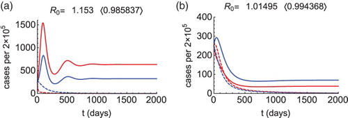
Our results for the control approaches (A) and (C) are illustrated in Figure 1. In the numerical simulations, we let ${\mathrm{\Lambda }}_i\left(N_i\right)=d_i{N}_i$, so the total population of the two patches (denoted here by $N^{\ast }$) is constant. In the DFE it must hold that $m_{12}{\overline{N}}_1=m_{21}{\overline{N}}_2$, that is ensured with $N_1\left(0\right)=m_{12}{N}^{\ast }/(m_{12}+m_{21})$, $N_2\left(0\right)=m_{21}{N}^{\ast }/(m_{12}+m_{21})$. We let $I_i\left(0\right)=250$, $R_i\left(0\right)=0$, $S_i\left(0\right)=N_i\left(0\right)-I_i\left(0\right)$ for the initial conditions, and choose parameter values as $N^{\ast }=2\cdot {10}^5$, $1/d_i=70$ years, $1/{\gamma }_i=5$ days, ${\theta }_i=200d_i$ ($i=1,2$), ${\mathcal{R}}_1=1.2$, ${\mathcal{R}}_2=1.05$, $m_{12}=0.015$, $m_{21}=0.015$, that makes ${\mathcal{R}}_0=1.153$. Figure 1(a) shows that reducing ${\beta }_1$ is sufficient for disease elimination if the condition (2(1) $\frac{1}{2}\left(\frac{{\beta }_2}{{\gamma }_2+m_{12}}+\sqrt{{\left(\frac{{\beta }_2}{{\gamma }_2+m_{12}}\right)}^2+\frac{4m_{12}{m}_{21}}{({\gamma }_2+m_{12})({\gamma }_1+m_{21})}}\right)<1.$(1) ) is satisfied. If, however, a higher outflow rate $m_{21}=0.1$ from the patch 1 is considered, then the condition (2(1) $\frac{1}{2}\left(\frac{{\beta }_2}{{\gamma }_2+m_{12}}+\sqrt{{\left(\frac{{\beta }_2}{{\gamma }_2+m_{12}}\right)}^2+\frac{4m_{12}{m}_{21}}{({\gamma }_2+m_{12})({\gamma }_1+m_{21})}}\right)<1.$(1) ) does not hold, yet ${\mathcal{R}}_0=1.07455>1$ and a different approach is necessary. As illustrated in Figure 1(b), the condition (4(3) $\rho (\tilde{\mathbf{K}}-{\tilde{\mathbf{K}}}_{\mathbf{W}})=\frac{{\beta }_2}{{\gamma }_2+m_{12}}<1$(3) ) is satisfied and the approach (C) can be applied, that includes the control of $m_{21}$ and ${\beta }_1$.

Figure 1. Morbidity curves of patch 1 (red) and patch 2 (blue), without control (solid curves) and with control (dashed curves). We let ${\mathcal{R}}_1=1.2$ (${\beta }_1=0.240047$), ${\mathcal{R}}_2=1.05$, $m_{12}=0.015$, and $m_{21}=0.015$ for (a) and $m_{21}=0.1$ for (b). Other parameters are as described in the text. Figure (a): When $m_{21}=0.015$, then ${\mathcal{R}}_0=1.153>1$ (solid curves), the condition (2(1) $\frac{1}{2}\left(\frac{{\beta }_2}{{\gamma }_2+m_{12}}+\sqrt{{\left(\frac{{\beta }_2}{{\gamma }_2+m_{12}}\right)}^2+\frac{4m_{12}{m}_{21}}{({\gamma }_2+m_{12})({\gamma }_1+m_{21})}}\right)<1.$(1) ) is satisfied ($0.981714<1$), so we calculate ${\mathcal{T}}_S=1.41186$ and ${\beta }_1^c=0.170022$. Choosing ${\beta }_1=0.1<{\beta }_1^c$ (dashed curves), the reproduction number drops below 1 (see in the bracket) and the outbreak is prevented. Figure (b): When $m_{21}=0.1$, then ${\mathcal{R}}_0=1.07455>1$ (solid curves), the condition (4(3) $\rho (\tilde{\mathbf{K}}-{\tilde{\mathbf{K}}}_{\mathbf{W}})=\frac{{\beta }_2}{{\gamma }_2+m_{12}}<1$(3) ) is satisfied ($0.976758<1$), so we calculate ${\mathcal{T}}_W=1.80031$ and ${\beta }_1^c=0.109093$, $m_{21}^c=0.0454465$. Choosing ${\beta }_1=0.1<{\beta }_1^c$ and $m_{21}=0.04<m_{21}^c$ (dashed curves), the reproduction number drops below 1 (see in the bracket) and the outbreak is prevented.

Despite the fact that in some cases changing only ${\beta }_1$ is sufficient for disease elimination, it is beneficial to include further parameters in the intervention strategy because it requires less effort. Following the terminology of Shuai et al. [15], the strategies defined by the sets W and U are stronger than S since $S\subset W$ and $S\subset U$. Then, by [15, Theorem 4.3] it holds that ${\mathcal{T}}_W<{\mathcal{T}}_S$ and ${\mathcal{T}}_U<{\mathcal{T}}_S$, provided that the target reproduction numbers are well defined (that is, the conditions for the controllability are satisfied). For each strategy, the controlled transmission rate ${\beta }_1^c$ is defined as we divide ${\beta }_1$ by the target reproduction number. Hence, the relationship between ${\mathcal{T}}_W$, ${\mathcal{T}}_U$, and ${\mathcal{T}}_S$ implies that in the strategy S that changes only ${\beta }_1$, the transmission rate needs to be decreased more compared to when other parameters are also involved (${\beta }_2$ in the strategy U, and $m_{21}$ in the strategy W). Moreover, the conditions for controllability (3(2) $\rho (\tilde{\mathbf{K}}-{\tilde{\mathbf{K}}}_{\mathbf{U}})<1⟺\sqrt{\frac{m_{12}{m}_{21}}{({\gamma }_2+m_{12})({\gamma }_1+m_{21})}}<1,$(2) ) and (4(3) $\rho (\tilde{\mathbf{K}}-{\tilde{\mathbf{K}}}_{\mathbf{W}})=\frac{{\beta }_2}{{\gamma }_2+m_{12}}<1$(3) ) in the strategies U and W, respectively, are less restrictive than the condition (2(1) $\frac{1}{2}\left(\frac{{\beta }_2}{{\gamma }_2+m_{12}}+\sqrt{{\left(\frac{{\beta }_2}{{\gamma }_2+m_{12}}\right)}^2+\frac{4m_{12}{m}_{21}}{({\gamma }_2+m_{12})({\gamma }_1+m_{21})}}\right)<1.$(1) ) in the strategy S, that means that stronger strategies can be applied more widely.

3.3. The approach (B)

We investigate the approach (B) for the control of the epidemic with changing the travel rates exclusively. We first show two situations when movement has no effect on whether an outbreak occurs. A standard result for nonnegative matrices (see, e.g. [12, Theorem 1.1]) says that the dominant eigenvalue of a nonnegative matrix is bounded below and above by the minimum and maximum of its column sums. Using basic calculus, we derive bounds for the column sums of $\tilde{\mathbf{K}}$ as $\begin{array}{rl}1& <\frac{{\beta }_1+m_{21}}{{\gamma }_1+m_{21}}\le \frac{{\beta }_1}{{\gamma }_1}={\mathcal{R}}_1\text{if}{\beta }_1-{\gamma }_1>0,\\ {\mathcal{R}}_1=\frac{{\beta }_1}{{\gamma }_1}& \le \frac{{\beta }_1+m_{21}}{{\gamma }_1+m_{21}}<1\text{if}{\beta }_1-{\gamma }_1<0,\end{array}$ and $\begin{array}{rl}1& <\frac{{\beta }_2+m_{12}}{{\gamma }_2+m_{12}}\le \frac{{\beta }_2}{{\gamma }_2}={\mathcal{R}}_2\text{if}{\beta }_2-{\gamma }_2>0,\\ {\mathcal{R}}_2& =\frac{{\beta }_2}{{\gamma }_2}\le \frac{{\beta }_2+m_{12}}{{\gamma }_2+m_{12}}<1\text{if}{\beta }_2-{\gamma }_2<0.\end{array}$ Thus, if ${\mathcal{R}}_1={\beta }_1/{\gamma }_1>1$ and ${\mathcal{R}}_2={\beta }_2/{\gamma }_2>1$ then the dominant eigenvalue of $\tilde{\mathbf{K}}$ is larger than 1, that also implies ${\mathcal{R}}_0>1$; with other words, if both local reproduction numbers are greater than 1 then so is ${\mathcal{R}}_0$, and no travel rates can reduce it below 1. On the other hand, when both ${\mathcal{R}}_1$ and ${\mathcal{R}}_2$ are less than 1 then it holds for every $m_{12},m_{21}$ that $\rho \left(\tilde{\mathbf{K}}\right)<1$ which is equivalent to ${\mathcal{R}}_0<1$, so the DFE is locally asymptotically stable and movement is unable to destabilize the situation.

If, however, ${\mathcal{R}}_1<1$ but ${\mathcal{R}}_2>1$ then ${\mathcal{R}}_1\le \rho \left(\tilde{\mathbf{K}}\right)\le {\mathcal{R}}_2$, and epidemic control might be necessary. In fact, with the approach (C) we are unable to apply the method of the target reproduction number on the alternative NGM $\tilde{\mathbf{K}}$. The approach (C) targets one or both of the travel rates, so assume without loss of generality that $m_{12}$ is subject to change. For those two entries of $\tilde{\mathbf{K}}$ that depend on this parameter, we note that the monotonicity of $[\tilde{\mathbf{K}}{]}_{1,2}$ in $m_{12}$ is opposite of that of $[\tilde{\mathbf{K}}{]}_{2,2}$. This means that the procedure of reducing related entries of $\tilde{\mathbf{K}}$ cannot be successful without controlling ${\beta }_2$ and/or ${\gamma }_2$.

We can, however, use another alternative NGM, that has the same properties as $\mathbf{K}$ and $\tilde{\mathbf{K}}$. Define $\breve{\mathbf{F}}=\left(\begin{array}{cc}{\beta }_1& 0\\ 0& {\beta }_2-{\gamma }_2\end{array}\right),\breve{\mathbf{V}}=\left(\begin{array}{cc}{\gamma }_1+m_{21}& -m_{12}\\ -m_{21}& m_{12}\end{array}\right),$ that satisfy $\mathbf{J}\mathbf{=}\stackrel{\mathbf{˘}}{\mathbf{F}}\mathbf{-}\stackrel{\mathbf{˘}}{\mathbf{V}}$, and $\breve{\mathbf{F}}$ is a nonnegative matrix by ${\mathcal{R}}_2={\beta }_2/{\gamma }_2>1$. If there is no travel outflow from the patch 2 then it is clear from ${\mathcal{R}}_2>1$ that the outbreak cannot be prevented. Otherwise, $m_{12}\ne 0$ and $\breve{\mathbf{V}}$ is a non-singular M-matrix, with nonnegative inverse. Thus, $\breve{\mathbf{K}}:=\breve{\mathbf{F}}\cdot {\breve{\mathbf{V}}}^{-1}$ gives an alternative NGM, which is also irreducible. $\breve{K}=\left(\begin{array}{cc}\frac{{\beta }_1}{{\gamma }_1}& \frac{{\beta }_1}{{\gamma }_1}\\ \frac{({\beta }_2-{\gamma }_2)m_{21}}{{\gamma }_1{m}_{12}}& \frac{({\beta }_2-{\gamma }_2)({\gamma }_1+m_{21})}{{\gamma }_1{m}_{12}}\end{array}\right).$ Our target set is $Z=\left\{\right(2,1),(2,2\left)\right\}$, the target matrix ${\breve{\mathbf{K}}}_{\mathbf{Z}}$ is given by $[{\breve{\mathbf{K}}}_{\mathbf{Z}}{]}_{1,1}=0$, $[{\breve{\mathbf{K}}}_{\mathbf{Z}}{]}_{1,2}=0$, $[{\breve{\mathbf{K}}}_{\mathbf{Z}}{]}_{2,1}=\left(\right({\beta }_2-{\gamma }_2\left)m_{21}\right)/{\gamma }_1{m}_{12}$, $[{\breve{\mathbf{K}}}_{\mathbf{Z}}{]}_{2,2}=({\beta }_2-{\gamma }_2)({\gamma }_1+m_{21})/{\gamma }_1{m}_{12}$, and the controllability condition reads (4) $\rho (\breve{\mathbf{K}}-{\breve{\mathbf{K}}}_{\mathbf{Z}})=\frac{{\beta }_1}{{\gamma }_1}<1,$(4) that holds since ${\mathcal{R}}_1<1$. The target reproduction number is calculated as $\begin{array}{rl}{\mathcal{T}}_Z& =\rho \left(\left(\begin{array}{cc}0& 0\\ \frac{({\beta }_2-{\gamma }_2)m_{21}}{{\gamma }_1{m}_{12}}& \frac{({\beta }_2-{\gamma }_2)({\gamma }_1+m_{21})}{{\gamma }_1{m}_{12}}\end{array}\right)\cdot {\left(\begin{array}{cc}1-\frac{{\beta }_1}{{\gamma }_1}& -\frac{{\beta }_1}{{\gamma }_1}\\ 0& 1\end{array}\right)}^{-1}\right)\\ & =\frac{{\beta }_1({\beta }_2-{\gamma }_2)m_{21}}{m_{12}{\gamma }_1({\gamma }_1-{\beta }_1)}+\frac{({\beta }_2-{\gamma }_2)({\gamma }_1+m_{21})}{{\gamma }_1{m}_{12}},\end{array}$ and by Proposition 2.1, ${\mathcal{R}}_0>1$ is equivalent to $\rho \left(\breve{\mathbf{K}}\right)>1$, hence ${\mathcal{T}}_Z>1$ (see [15, Theoreom 2.1]).

The controlled matrix ${\breve{\mathbf{K}}}_{\mathbf{c}}$ corresponding to the strategy Z, is defined by $[{\breve{\mathbf{K}}}_{\mathbf{c}}{]}_{2,i}=[\breve{\mathbf{K}}{]}_{2,i}/{\mathcal{T}}_Z$, $i=1,2$, while control does not affect the first row of $\breve{\mathbf{K}}$. To determine how this transformation of $\breve{\mathbf{K}}$ is achieved in terms of the targeted parameters, we need to derive $m_{12}^c$ and $m_{21}^c$ that satisfy $[{\breve{\mathbf{K}}}_{\mathbf{c}}{]}_{2,i}=[\breve{\mathbf{K}}{]}_{2,i}(m_{12}^c,m_{21}^c)$, $i=1,2$. To this end, we solve the system $\begin{array}{rl}\frac{({\beta }_2-{\gamma }_2)m_{21}}{{\mathcal{T}}_Z\cdot {\gamma }_1{m}_{12}}& =\frac{({\beta }_2-{\gamma }_2)m_{21}^c}{{\gamma }_1{m}_{12}^c},\\ \frac{({\beta }_2-{\gamma }_2)({\gamma }_1+m_{21})}{{\mathcal{T}}_Z\cdot {\gamma }_1{m}_{12}}& =\frac{({\beta }_2-{\gamma }_2)({\gamma }_1+m_{21}^c)}{{\gamma }_1{m}_{12}^c},\end{array}$ that reduces to $\begin{array}{rl}\frac{m_{21}}{{\mathcal{T}}_Z\cdot m_{12}}& =\frac{m_{21}^c}{m_{12}^c},\\ \frac{{\gamma }_1}{{\mathcal{T}}_Z\cdot m_{12}}& =\frac{{\gamma }_1}{m_{12}^c}.\end{array}$ It follows that $m_{12}^c={\mathcal{T}}_Z\cdot m_{12}$ and $m_{21}^c=m_{21}$, which means that the travel inflow rate into patch 1 with ${\mathcal{R}}_1<1$ (that rate is also the travel outflow rate of patch 2 with ${\mathcal{R}}_2>1$) needs to be increased, and the other travel rate must remain unchanged.

We close this section with some concluding remarks. Three control approaches were investigated for the SIRS model with individuals' travel between two patches. Intervention strategies that target transmissibility are powerful tools in epidemic control; as shown in this section, preventing outbreaks by reducing the transmission rates ${\beta }_1$ and ${\beta }_2$, is possible for any movement rates and for any value of the basic reproduction number ${\mathcal{R}}_0$. We also described cases in the approach (A) when changing (reducing) only one of the transmission rates is sufficient, and showed that allowing the additional control of travel rates requires less effort. In particular, if ${\mathcal{R}}_1,{\mathcal{R}}_2<1$ then ${\mathcal{R}}_0<1$ and no control is necessary, but if $max({\mathcal{R}}_1,{\mathcal{R}}_2)>1$ and ${\mathcal{R}}_0>1$ then bringing the basic reproduction number below 1 is possible by targeting ${\beta }_1$ and $m_{21}$ if ${\beta }_2/{\gamma }_2+m_{12}<1$ holds. Hence, the approach (C) is successful if ${\mathcal{R}}_1>1$ and ${\mathcal{R}}_2<1$ (since ${\mathcal{R}}_2={\beta }_2/{\gamma }_2\ge {\beta }_2/{\gamma }_2+m_{12}$), but more interestingly, the strategy might also be feasible even when ${\mathcal{R}}_2>1$, if $m_{12}$ is such that ${\beta }_2/{\gamma }_2+m_{12}<1$. 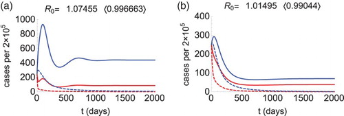Biologically, the case when ${\mathcal{R}}_1<1$, ${\mathcal{R}}_2>1$, and ${\beta }_2/{\gamma }_2+m_{12}<1$ means that if the travel rate from an endemic area (patch 2) is large enough, then disease control is feasible by decreasing the transmission rate in the non-endemic patch (patch 1) and reducing the travel inflow to the endemic area. See Figure 2(a) that illustrates this phenomenon. We let ${\mathcal{R}}_1=0.95$, ${\mathcal{R}}_2=1.05$, $m_{12}=0.015$, $m_{21}=0.015$, and other parameters are as described for Figure 1.

Figure 2. Morbidity curves of patch 1 (red) and patch 2 (blue), without control (solid curves) and with control (dashed curves). We let ${\mathcal{R}}_1=0.95$ (${\beta }_1=0.190037$), ${\mathcal{R}}_2=1.05$, $m_{12}=0.015$, $m_{21}=0.015$. Other parameters are as described in the text. These parameters make ${\mathcal{R}}_0=1.01495>1$ (solid curves). Figure (a): The condition (4(3) $\rho (\tilde{\mathbf{K}}-{\tilde{\mathbf{K}}}_{\mathbf{W}})=\frac{{\beta }_2}{{\gamma }_2+m_{12}}<1$(3) ) is satisfied ($0.976758<1$), so we calculate ${\mathcal{T}}_W=1.01495$, and ${\beta }_1^c=0.172752$, $m_{21}^c=0.0136356$. Choosing ${\beta }_1=0.15<{\beta }_1^c$ and $m_{21}=0.012<m_{21}^c$ (dashed curves), the reproduction number drops below 1 (see in the bracket) and the outbreak is prevented. Figure (b): The condition (5(4) $\rho (\breve{\mathbf{K}}-{\breve{\mathbf{K}}}_{\mathbf{Z}})=\frac{{\beta }_1}{{\gamma }_1}<1,$(4) ) is satisfied (${\mathcal{R}}_1<1$), so we calculate ${\mathcal{T}}_Z=1.66667$, and $m_{12}^c=0.025$. Choosing $m_{12}=0.03>m_{21}^c$ (dashed curves), the reproduction number drops below 1 (see in the bracket) and the outbreak is prevented.

Lastly, we investigated for the approach (B) whether epidemic control is possible without changing any of the transmission rates. If both local reproduction numbers are greater than 1 then it is impossible for movement to prevent the outbreak, since ${\mathcal{R}}_0$ is greater than 1 for any travel rates. On the other hand, we learned that ${\mathcal{R}}_0$ can be reduced to 1 by increasing the inflow rate to a patch where the local reproduction number is less than 1. Figure 2(b) illustrates such a case, where ${\mathcal{R}}_1=0.95<1$, ${\mathcal{R}}_2=1.05>1$, and ${\mathcal{R}}_0=1.01495>1$, so we increase $m_{12}$ to eliminate the disease. We point out that if both local reproduction numbers are below 1 then movement cannot destabilize the DFE, hence no outbreak will occur.

4. A generalized SIRS model for r patches

In this section, control strategies are investigated in a general demographic SIRS model with individuals' travel between r patches, where $r\ge 2$ is positive integer. Understanding the dynamics of such high-dimensional models remains a challenging problem in mathematical epidemiology. We give the system of $3r$ ODEs (M2) $\begin{array}{rl}{S}_i^{\prime }& ={\mathrm{\Lambda }}_i\left(N_i\right)-{\beta }_i\frac{S_i{I}_i}{N_i}-d_i{S}_i+{\theta }_i{R}_i-\sum _{j=1}^r{m}_{ji}^S{S}_i+\sum _{j=1}^r{m}_{ij}^S{S}_j,\\ I_i^{\prime }& ={\beta }_i\frac{S_i{I}_i}{N_i}-({\alpha }_i+{\delta }_i+d_i)I_i-\sum _{j=1}^r{m}_{ji}^I{I}_i+\sum _{j=1}^r{m}_{ij}^I{I}_j,i=1,\dots ,r.\\ R_i^{\prime }& ={\alpha }_i{I}_i-({\theta }_i+d_i)R_i-\sum _{j=1}^r{m}_{ji}^R{R}_i+\sum _{j=1}^r{m}_{ij}^R{R}_j.\end{array}$(M2) The parameter $m_{ji}^X$ is the travel rate in the class X, from region i to j ($X\in \{S,I,R\}$, $i,j\in \{1,\dots ,r\}$, $j\ne i$), and we define $m_{ii}^X=0$ for $i=1,\dots ,r$, $X=S,I,R$. Besides that we allow different movement rates of the three disease classes, it is also incorporated that the disease increases mortality by rate ${\delta }_i>0$. All other parameters, model variables and functions have been introduced in Section 2. Following the arguments made for a similar model in [6], we assume that there is a unique DFE $({\overline{N}}_1,0,0,\dots ,{\overline{N}}_r,0,0)$ in the model (6(M2) $\begin{array}{rl}{S}_i^{\prime }& ={\mathrm{\Lambda }}_i\left(N_i\right)-{\beta }_i\frac{S_i{I}_i}{N_i}-d_i{S}_i+{\theta }_i{R}_i-\sum _{j=1}^r{m}_{ji}^S{S}_i+\sum _{j=1}^r{m}_{ij}^S{S}_j,\\ I_i^{\prime }& ={\beta }_i\frac{S_i{I}_i}{N_i}-({\alpha }_i+{\delta }_i+d_i)I_i-\sum _{j=1}^r{m}_{ji}^I{I}_i+\sum _{j=1}^r{m}_{ij}^I{I}_j,i=1,\dots ,r.\\ R_i^{\prime }& ={\alpha }_i{I}_i-({\theta }_i+d_i)R_i-\sum _{j=1}^r{m}_{ji}^R{R}_i+\sum _{j=1}^r{m}_{ij}^R{R}_j.\end{array}$(M2) ). With ${\gamma }_i={\alpha }_i+{\delta }_i+d_i$, we define the local reproduction number of patch i as ${\mathcal{R}}_i=\frac{{\beta }_i}{{\gamma }_i}$. With $m_{ij}:=m_{ij}^I$, the infected subsystem is obtained as $I_i^{\prime }={\beta }_i\frac{S_i{I}_i}{N_i}-{\gamma }_i{I}_i-\sum _{j=1}^r{m}_{ji}{I}_i+\sum _{j=1}^r{m}_{ij}{I}_j,i=1,\dots ,r.$ We define $\mathbf{M}$ as the movement matrix of infected individuals, and $M_i$ as the total outflow of infected individuals from region i, $i\in \{1,\dots ,r\}$: $\begin{array}{rl}\mathbf{M}& =(m_{ji}{)}^{r\times r},\\ M_i& =\sum _{\begin{array}{c}j=1\\ j\ne i\end{array}}^r{m}_{ji}.\end{array}$ In the sequel, we will simply say ‘movement matrix’ for $\mathbf{M}$ and ‘total outflow from region i’ for $M_i$, and the reference to infected individuals will be omitted. It is reasonable to assume that $\mathbf{M}$ is irreducible. Otherwise, the patches are not strongly connected with respect to the disease, so a subsets of the patches can be constructed to where the epidemic cannot spread from other patches. Linearization of the infected subsystem about the DFE gives the Jacobian $\mathbf{J}\in {\mathbb{R}}^{\mathbf{r}\times \mathbf{r}}$, as $\mathbf{J}\mathbf{=}\mathrm{diag}\mathbf{(}{\beta }_{\mathbf{1}}\mathbf{-}{\gamma }_{\mathbf{1}}\mathbf{-}{\mathbf{M}}_{\mathbf{1}}\mathbf{,}\dots \mathbf{,}{\beta }_{\mathbf{r}}\mathbf{-}{\gamma }_{\mathbf{r}}\mathbf{-}{\mathbf{M}}_{\mathbf{r}}\mathbf{)}\mathbf{+}\mathbf{M}\mathbf{.}$ The basic reproduction number is defined as we follow the usual procedure of decomposing the Jacobian as $\mathbf{F}\mathbf{-}\mathbf{V}$, where $\mathbf{F}\mathbf{=}\mathrm{diag}\mathbf{(}{\beta }_{\mathbf{1}}\mathbf{,}\dots \mathbf{,}{\beta }_{\mathbf{r}}\mathbf{)}\mathbf{,}\mathbf{V}\mathbf{=}\mathrm{diag}\mathbf{(}{\gamma }_{\mathbf{1}}\mathbf{+}{\mathbf{M}}_{\mathbf{1}}\mathbf{,}\dots \mathbf{,}{\gamma }_{\mathbf{r}}\mathbf{+}{\mathbf{M}}_{\mathbf{r}}\mathbf{)}\mathbf{-}\mathbf{M}\mathbf{,}$ $\mathbf{F}$ is the matrix representing new infections and $\mathbf{V}$ represents transitions between and out of infected classes. It is easy to see that $\mathbf{F}\ge \mathbf{0}$ and $\mathbf{V}$ has the Z-sign pattern. As $\mathbf{V}$ is diagonally dominant, the equivalence of the properties 3 and 11 in [9, Theorem 5.1] implies that ${\mathbf{V}}^{\mathbf{-}\mathbf{1}}$ exists and it is nonnegative. Following van den Driessche and Watmough [17], the basic reproduction number ${\mathcal{R}}_0$ is defined as the dominant eigenvalue of the NGM $\mathbf{K}\mathbf{:=}\mathbf{F}\cdot {\mathbf{V}}^{\mathbf{-}\mathbf{1}}$, that is, ${\mathcal{R}}_0=\rho \left(\mathbf{K}\mathbf{\right)}\mathbf{=}\rho \mathbf{(}\mathbf{F}\cdot {\mathbf{V}}^{\mathbf{-}\mathbf{1}}\mathbf{)}$. Note that the entries of ${\mathbf{V}}^{\mathbf{-}\mathbf{1}}$ and $\mathbf{K}$ arise by complicated expressions, and hence no closed formula is derived for ${\mathcal{R}}_0$.

An alternative way to decompose the Jacobian is $\mathbf{J}\mathbf{=}\stackrel{\mathbf{~}}{\mathbf{F}}\mathbf{-}\stackrel{\mathbf{~}}{\mathbf{V}}$, where $\tilde{\mathbf{F}}=\mathrm{diag}({\beta }_1,\dots ,{\beta }_r)+\mathbf{M}\mathbf{,}\stackrel{\mathbf{~}}{\mathbf{V}}\mathbf{=}\mathrm{diag}\mathbf{(}{\gamma }_{\mathbf{1}}\mathbf{+}{\mathbf{M}}_{\mathbf{1}}\mathbf{,}\dots \mathbf{,}{\gamma }_{\mathbf{r}}\mathbf{+}{\mathbf{M}}_{\mathbf{r}}\mathbf{)}\mathbf{.}$ $\tilde{\mathbf{F}}$ is nonnegative and $\tilde{\mathbf{V}}$ has the Z-sign pattern, so with $\tilde{\mathbf{K}}:=\tilde{\mathbf{F}}\cdot {\tilde{\mathbf{V}}}^{-1}$ an alternative NGM arises. By Proposition 2.1, $\rho \left(\tilde{\mathbf{K}}\right)$ gives another threshold quantity for the stability of the DFE; more precisely, $\rho \left(\tilde{\mathbf{K}}\right)<1$ if and only if ${\mathcal{R}}_0<1$, $\rho \left(\tilde{\mathbf{K}}\right)=1$ if and only if ${\mathcal{R}}_0=1$, and $\rho \left(\tilde{\mathbf{K}}\right)>1$ if and only if ${\mathcal{R}}_0>1$. The alternative NGM $\tilde{\mathbf{K}}$ is obtained as $\begin{array}{rl}\tilde{\mathbf{K}}& =\left(\begin{array}{cccc}\frac{{\beta }_1}{{\gamma }_1+M_1}& \frac{m_{12}}{{\gamma }_2+M_2}& \cdots & \frac{m_{1r}}{{\gamma }_r+M_r}\\ \frac{m_{21}}{{\gamma }_1+M_1}& \frac{{\beta }_2}{{\gamma }_2+M_2}& \cdots & \frac{m_{2r}}{{\gamma }_r+M_r}\\ ⋮& ⋮& \ddots & ⋮\\ \frac{m_{r1}}{{\gamma }_1+M_1}& \frac{m_{r2}}{{\gamma }_2+M_2}& \cdots & \frac{{\beta }_r}{{\gamma }_r+M_r}\end{array}\right),\end{array}$ that is irreducible since $\mathbf{M}$ is irreducible.

Assume that the disease can invade into the population and ${\mathcal{R}}_0>1$, that is equivalent to $\rho \left(\tilde{\mathbf{K}}\right)>1$ (see Proposition 2.1). Intervention strategies can potentially target:

1. various transmission rates;

2. various movement rates;

3. the combination of the above, in frames of local control.

For the model (1(M1) $\begin{array}{rl}{S}_1^{\prime }& ={\mathrm{\Lambda }}_1\left(N_1\right)-{\beta }_1\frac{S_1{I}_1}{N_1}-d_1{S}_1+{\theta }_1{R}_1-m_{21}{S}_1+m_{12}{S}_2,\\ I_1^{\prime }& ={\beta }_1\frac{S_1{I}_1}{N_1}-({\alpha }_1+d_1)I_1-m_{21}{I}_1+m_{12}{I}_2,\\ R_1^{\prime }& ={\alpha }_1{I}_1-({\theta }_1+d_1)R_1-m_{21}{R}_1+m_{12}{R}_2,\\ S_2^{\prime }& ={\mathrm{\Lambda }}_2\left(N_2\right)-{\beta }_2\frac{S_2{I}_2}{N_2}-d_2{S}_2+{\theta }_2{R}_2-m_{12}{S}_2+m_{21}{S}_1,\\ I_2^{\prime }& ={\beta }_2\frac{S_2{I}_2}{N_2}-({\alpha }_2+d_2)I_2-m_{12}{I}_2+m_{21}{I}_1,\\ R_1^{\prime }& ={\alpha }_2{I}_2-({\theta }_2+d_2)R_2-m_{12}{R}_2+m_{21}{R}_1.\end{array}$(M1) ) in Section 3 for two patches, the control approaches (A), (B), and (C) have been thoroughly investigated. We derived precise conditions for controllability and described in details the procedures that lead to the decrease of ${\mathcal{R}}_0$ to 1 (that is, we gave the formulas for the targeted parameters in the various strategies). In this section, we present theorems that generalize to r regions our results obtained for the 2-patch SIRS model (1(M1) $\begin{array}{rl}{S}_1^{\prime }& ={\mathrm{\Lambda }}_1\left(N_1\right)-{\beta }_1\frac{S_1{I}_1}{N_1}-d_1{S}_1+{\theta }_1{R}_1-m_{21}{S}_1+m_{12}{S}_2,\\ I_1^{\prime }& ={\beta }_1\frac{S_1{I}_1}{N_1}-({\alpha }_1+d_1)I_1-m_{21}{I}_1+m_{12}{I}_2,\\ R_1^{\prime }& ={\alpha }_1{I}_1-({\theta }_1+d_1)R_1-m_{21}{R}_1+m_{12}{R}_2,\\ S_2^{\prime }& ={\mathrm{\Lambda }}_2\left(N_2\right)-{\beta }_2\frac{S_2{I}_2}{N_2}-d_2{S}_2+{\theta }_2{R}_2-m_{12}{S}_2+m_{21}{S}_1,\\ I_2^{\prime }& ={\beta }_2\frac{S_2{I}_2}{N_2}-({\alpha }_2+d_2)I_2-m_{12}{I}_2+m_{21}{I}_1,\\ R_1^{\prime }& ={\alpha }_2{I}_2-({\theta }_2+d_2)R_2-m_{12}{R}_2+m_{21}{R}_1.\end{array}$(M1) ). We also derive novel conclusions.

Proposition 4.1:

If ${\mathcal{R}}_0>1$ then there is at least one patch with local reproduction number greater than 1. If the local reproduction number is greater than 1 in all patches then it holds that $\rho \left(\tilde{\mathbf{K}}\right)>1,$ that is equivalent to ${\mathcal{R}}_0>1$.

Proof:

Indeed, we look at the column sums of $\tilde{\mathbf{K}}$ to give upper and lower bounds on the dominant eigenvalue. As the column sum in column j is $({\beta }_j+M_j)/({\gamma }_j+M_j)$, we derive by the result of Minc [12, Theorem 1.1] that $\underset{1\le j\le r}{min}\frac{{\beta }_j+M_j}{{\gamma }_j+M_j}\le \rho \left(\tilde{\mathbf{K}}\right)\le \underset{1\le j\le r}{max}\frac{{\beta }_j+M_j}{{\gamma }_j+M_j}.$ The expression $({\beta }_j+x)/({\gamma }_j+x)$ is increasing in x if ${\beta }_j<{\gamma }_j$, and it is bounded above by 1, hence if ${\mathcal{R}}_j={\beta }_j/{\gamma }_j<1$ for every $j\in \{1,\dots ,r\}$ then $\rho \left(\tilde{\mathbf{K}}\right)\le 1$ follows. The last inequality is equivalent to ${\mathcal{R}}_0\le 1$ that contradicts our assumption that ${\mathcal{R}}_0>1$, hence there must be an i such that ${\mathcal{R}}_i>1$.

On the other hand, $({\beta }_j+x)/({\gamma }_j+x)$ decreases in x if ${\beta }_j>{\gamma }_j$, and it is bounded below by 1. Summarizing, we have $\begin{array}{rl}1& <\frac{{\beta }_j+M_j}{{\gamma }_j+M_j}\le \frac{{\beta }_j}{{\gamma }_j}={\mathcal{R}}_j\text{if}{\beta }_j-{\gamma }_j>0,\\ {\mathcal{R}}_j& =\frac{{\beta }_j}{{\gamma }_j}\le \frac{{\beta }_j+M_j}{{\gamma }_j+M_j}<1\text{if}{\beta }_j-{\gamma }_j<0,\end{array}$ thus 1 gives the lower bound of $\rho \left(\tilde{\mathbf{K}}\right)$ if all local reproduction numbers are greater than 1. The last statement implies that if ${\mathcal{R}}_j>1$ in all patches then ${\mathcal{R}}_0$ is greater than 1 for any travel rates. This completes the proof.

Theorem 4.2 (For the approach (A))

The epidemic can be controlled by decreasing the transmission rate in some regions, if the local reproduction number is less than 1 in all other patches. This implies that decreasing the transmission rate in all regions with local reproduction numbers greater than 1, can be sufficient for epidemic control. In particular, the intervention strategy where all transmission rates are subject to change, leads to disease elimination.

Proof:

Since ${\mathcal{R}}_0>1$ by assumption, there is an $i\in \{1,\dots ,r\}$ such that ${\mathcal{R}}_i>1$. Without loss of generality, we can assume that ${\mathcal{R}}_i={\beta }_i/{\gamma }_i>1$ for $i=1,\dots ,p$ whereas ${\mathcal{R}}_j={\beta }_j/{\gamma }_j<1$ for $j=p+1,\dots ,r$ ($1\le p<r$).

First, consider that ${\beta }_1,\dots ,{\beta }_p$ are targeted and ${\beta }_{p+1},\dots ,{\beta }_r$ are not subject to change. The target set is $S=\left\{\right(1,1),\dots ,(p,p\left)\right\}$, the target matrix is ${\tilde{\mathbf{K}}}_{\mathbf{S}}=\mathrm{diag}({\beta }_1/(\gamma +M_1),\dots ,{\beta }_p/({\gamma }_p+M_p),0,\dots ,0)$, and the controllability condition reads (5) $\rho (\tilde{\mathbf{K}}-{\tilde{\mathbf{K}}}_{\mathbf{S}})<1.$(5) Column sums of the matrix $\tilde{\mathbf{K}}-{\tilde{\mathbf{K}}}_{\mathbf{S}}$ are calculated as $\frac{M_1}{{\gamma }_1+M_1},\dots \frac{M_p}{{\gamma }_p+M_p},\frac{{\beta }_{p+1}+M_{p+1}}{{\gamma }_{p+1}+M_{p+1}},\dots \frac{{\beta }_r+M_r}{{\gamma }_r+M_r}.$ Obviously, $M_i/({\gamma }_i+M_i)<1$ for $i=1,\dots ,p$, and it is easy to check that ${\beta }_j/{\gamma }_j\le ({\beta }_j+M_j)/({\gamma }_j+M_j)<1$ if ${\mathcal{R}}_j={\beta }_j/{\gamma }_j<1$, that implies that $({\beta }_j+M_j)/({\gamma }_j+M_j)<1$ for $j=p+1,\dots ,r$. It is known that the dominant eigenvalue of a nonnegative matrix is bounded above by the maximum of the column sums (see [12, Theorem 1.1]), so applying this result to $\tilde{\mathbf{K}}-{\tilde{\mathbf{K}}}_{\mathbf{S}}$ we obtain that the condition (7(5) $\rho (\tilde{\mathbf{K}}-{\tilde{\mathbf{K}}}_{\mathbf{S}})<1.$(5) ) for controllability holds.

The target reproduction number for the strategy S is given by ${\mathcal{T}}_S=\rho ({\tilde{\mathbf{K}}}_{\mathbf{S}}\cdot (\mathbf{I}-\tilde{\mathbf{K}}+{\tilde{\mathbf{K}}}_{\mathbf{S}}{)}^{-1}),$ and we define the controlled transmission rates as ${\beta }_i^c:={\beta }_i/{\mathcal{T}}_S$, $i=1,\dots ,p$. For $i=1,\dots ,p$, we replace ${\beta }_i$ by ${\beta }_i^c$ in $\tilde{\mathbf{K}}$ and arrive to the controlled matrix ${\tilde{\mathbf{K}}}_{\mathbf{c}}$, that satisfies $\rho \left({\tilde{\mathbf{K}}}_{\mathbf{c}}\right)=1$ (see [15, Theorem 2.2]). The assumption that ${\mathcal{R}}_0>1$ implies by Proposition 2.1 and [15, Theorem 2.1] that ${\mathcal{T}}_S>1$, hence targeted transmission rates need to be reduced for successful control.

Theorem 4.3 in [15] says that extending the control strategy to a wider set of entries of $\tilde{\mathbf{K}}$ requires less effort for disease elimination. If, in addition to ${\beta }_1,\dots ,{\beta }_p$, we also control the transmission rates ${\beta }_{p+1},\dots ,{\beta }_{p+q}$ ($q\ge 1$), then some regions with local reproduction numbers less than 1 are also targeted. However, it remains true that ${\mathcal{R}}_j<1$ for all $j>p+q$, that is, for all j such that ${\beta }_j$ is not subject to change. The target set is $U=\left\{\right(1,1),\dots ,(p+q,p+q\left)\right\}$, and the control strategy U is stronger than S because of $S\subset U$. Since ${\tilde{\mathbf{K}}}_{\mathbf{S}}\le {\tilde{\mathbf{K}}}_{\mathbf{U}}$, it holds that $\tilde{\mathbf{K}}-{\tilde{\mathbf{K}}}_{\mathbf{U}}\le \tilde{\mathbf{K}}-{\tilde{\mathbf{K}}}_{\mathbf{S}}$, and by a basic result on nonnegative matrices (see, for instance, [9, Lemma 4.6]) we obtain $\rho (\tilde{\mathbf{K}}-{\tilde{\mathbf{K}}}_{\mathbf{U}})<\rho (\tilde{\mathbf{K}}-{\tilde{\mathbf{K}}}_{\mathbf{S}})$, that implies that the strategy U is also feasible for control. Theorem 4.3 in [15] says $1<{\mathcal{T}}_U\le {\mathcal{T}}_S$, thus, stronger control strategies require less effort. Note that these conclusions are valid for the case when $p+q=r$, that is, when all transmission rates are targeted.

Theorem 4.3 (For the approach (C))

Local control in some regions, that involves the control of transmission rates and travel outflow of those regions, can be sufficient if $({\beta }_j+M_j)/({\gamma }_j+M_j)<1$ in all other regions. This implies that if all patches with $({\beta }_i+M_i)/({\gamma }_i+M_i)>1$ are under control then the outbreak can be prevented. In particular, the intervention strategy where all transmission rates and travel rates are subject to change, leads to disease elimination.

Proof:

We have seen that for ${\mathcal{R}}_0>1$ it is necessary that ${\mathcal{R}}_i>1$ for some i. As $1<({\beta }_i+M_i)/{\gamma }_i+M_i\le {\mathcal{R}}_i$ holds for any $M_i\ge 0$ if ${\mathcal{R}}_i>1$, we can assume without loss of generality that there is a $p\ge 1$ such that $({\beta }_i+M_i)/({\gamma }_i+M_i)>1$ for $i=1,\dots ,p$, and $({\beta }_j+M_j)/({\gamma }_j+M_j)<1$ for $j=p+1,\dots ,r$.

If the patches $1,\dots ,p$ are under local control, then the parameters ${\beta }_i$ and $m_{ji}$ are subject to change, where $i\in \{1,\dots ,p\}$, $j\in \{1,\dots ,r\}$, $j\ne i$, so we introduce $\mathrm{\Omega }={\cup }_{i=1}^p{\cup }_{j=1}^r\{{\beta }_i,m_{ji}\}$ for the set of targeted parameters. The target set (of entries in the NGM $\tilde{\mathbf{K}}$) is $W=\left\{\right(j,1),\dots ,(j,p\left)\right\}$ with $j\in \{1,\dots ,r\}$, the target matrix ${\tilde{\mathbf{K}}}_{\mathbf{W}}$ is defined as $[{\tilde{\mathbf{K}}}_{\mathbf{W}}{]}_{j,i}=[\tilde{\mathbf{K}}{]}_{j,i}$ if $i\in \{1,\dots ,p\}$ and 0 otherwise, and the controllability condition reads (6) $\rho (\tilde{\mathbf{K}}-{\tilde{\mathbf{K}}}_{\mathbf{W}})<1.$(6) The matrix $\tilde{\mathbf{K}}-{\tilde{\mathbf{K}}}_{\mathbf{W}}$ is lower triangular with a zero-block in the diagonal and another diagonal block of size $(r-p)\times (r-p)$, that we denote by $\mathbf{B}$: $\tilde{\mathbf{K}}-{\tilde{\mathbf{K}}}_{\mathbf{W}}=\left(\begin{array}{cc}0& \ast \\ 0& B\end{array}\right),\mathbf{B}=\left(\begin{array}{cccc}\frac{{\beta }_{p+1}}{{\gamma }_{p+1}+M_{p+1}}& \frac{m_{p+1,p+2}}{{\gamma }_{p+2}+M_{p+2}}& \cdots & \frac{m_{p+1,r}}{{\gamma }_r+M_r}\\ \frac{m_{p+2,p+1}}{{\gamma }_{p+1}+M_{p+1}}& \frac{{\beta }_{p+2}}{{\gamma }_{p+2}+M_{p+2}}& \cdots & \frac{m_{p+2,r}}{{\gamma }_r+M_r}\\ ⋮& ⋮& \ddots & ⋮\\ \frac{m_{r,p+1}}{{\gamma }_{p+1}+M_{p+1}}& \frac{m_{r,p+2}}{{\gamma }_{p+2}+M_{p+2}}& \cdots & \frac{{\beta }_r}{{\gamma }_r+M_r}\end{array}\right).$ Due to the special structure of $\tilde{\mathbf{K}}-{\tilde{\mathbf{K}}}_{\mathbf{W}}$, the dominant eigenvalue arises as the dominant eigenvalue of the square matrix $\mathbf{B}$. Again, by [12, Theorem 1.1] and the assumption that $({\beta }_j+M_j)/({\gamma }_j+M_j)<1$ for $j=p+1,\dots ,r$, we obtain that $\begin{array}{rl}\rho (\tilde{\mathbf{K}}-{\tilde{\mathbf{K}}}_{\mathbf{W}})=\rho \left(\mathbf{B}\right)& \le \underset{p+1\le j\le r}{max}\left(\frac{{\beta }_j+\sum _{i=p+1}^r{m}_{ij}}{{\gamma }_j+M_j}\right)\\ & \le \underset{p+1\le j\le r}{max}\left(\frac{{\beta }_j+M_j}{{\gamma }_j+M_j}\right)\\ & <1,\end{array}$ that implies that the controllability condition (8(6) $\rho (\tilde{\mathbf{K}}-{\tilde{\mathbf{K}}}_{\mathbf{W}})<1.$(6) ) holds. We can thus define the target reproduction number ${\mathcal{T}}_W=\rho ({\tilde{\mathbf{K}}}_{\mathbf{W}}\cdot (\mathbf{I}-\tilde{\mathbf{K}}+{\tilde{\mathbf{K}}}_{\mathbf{W}}{)}^{-1})$ for the strategy W, that is greater than 1 because of $\rho \left(\tilde{\mathbf{K}}\right)>1$. For successful control, each parameter in the set $\mathrm{\Omega }={\cup }_{i=1}^p{\cup }_{j=1}^r\{{\beta }_i,m_{ji}\}$ needs to be changed such that $\left[\tilde{\mathbf{K}}\right({\mathrm{\Omega }}_c){]}_{j,i}=[\tilde{\mathbf{K}}\left(\mathrm{\Omega }\right){]}_{j,i}/{\mathcal{T}}_W$ for $(j,i)\in W$, where ${\mathrm{\Omega }}_c$ is the set of targeted parameters after the control. This way, $\tilde{\mathbf{K}}\left({\mathrm{\Omega }}_c\right)$ is equal to the controlled next-generation matrix ${\tilde{\mathbf{K}}}_{\mathbf{c}}$, and $\tilde{\mathbf{K}}\left({\mathrm{\Omega }}_c\right)=1$ follows from $\rho \left({\tilde{\mathbf{K}}}_{\mathbf{c}}\right)=1$ (see [15, Theorem 2.2]).

Controlled parameters need to satisfy the systems $\begin{array}{r}\left\{\begin{array}{l}\frac{{\beta }_1^c}{{\gamma }_1+M_1^c}=\frac{{\beta }_1}{({\gamma }_1+M_1){\mathcal{T}}_W},\\ \frac{m_{21}^c}{{\gamma }_1+M_1^c}=\frac{m_{21}}{({\gamma }_1+M_1){\mathcal{T}}_W},\\ ⋮\\ \frac{m_{r1}^c}{{\gamma }_1+M_1^c}=\frac{m_{r1}}{({\gamma }_1+M_1){\mathcal{T}}_W},\end{array}\right.\dots \left\{\begin{array}{l}\frac{{\beta }_p^c}{{\gamma }_p+M_p^c}=\frac{{\beta }_p}{({\gamma }_p+M_p){\mathcal{T}}_W},\\ \frac{m_{1p}^c}{{\gamma }_p+M_p^c}=\frac{m_{1p}}{({\gamma }_p+M_p){\mathcal{T}}_W},\\ ⋮\\ \frac{m_{rp}^c}{{\gamma }_p+M_p^c}=\frac{m_{rp}}{({\gamma }_p+M_p){\mathcal{T}}_W},\end{array}\right.\end{array}$ that are pairwise independent so it is sufficient to solve one of them (e.g. the first one), and then generalize. To find the controlled parameters ${\beta }_1^c,m_{21}^c,\dots ,m_{r1}^c$, we first solve the system $\begin{array}{rl}\frac{m_{21}^c}{{\gamma }_1+M_1^c}& =\frac{m_{21}}{({\gamma }_1+M_1){\mathcal{T}}_W},\\ & ⋮\\ \frac{m_{r1}^c}{{\gamma }_1+M_1^c}& =\frac{m_{r1}}{({\gamma }_1+M_1){\mathcal{T}}_W},\end{array}$ where $M_1^c=\sum _{j=2}^r{m}_{j1}^c$. We obtain that $m_{j1}^c/m_{j1}=m_{k1}^c/m_{k1}$ whenever $m_{j1}\ne 0$, $m_{k1}\ne 0$, thus there is a $c_1$ such that $m_{j1}^c=m_{j1}/c_1$ for every j such that $m_{j1}\ne 0$. If $m_{j1}=0$ for some j then define $m_{j1}^c=0$. It follows that $M_1^c=M_1/c_1$, and $m_{j1}/c_1/{\gamma }_1+M_1/c_1=m_{j1}/({\gamma }_1+M_1){\mathcal{T}}_W$ has to be satisfied, so $c_1$ is given by $c_1=\left(\right({\gamma }_1+M_1){\mathcal{T}}_S-M_1)/{\gamma }_1$. It is easy to see that $c_1>1$, which means that travel outflow rates from patch 1 need to be decreased for disease elimination. However, the transmission rate of patch 1 needs to be changed such that $\frac{{\beta }_1^c}{{\gamma }_1+M_1^c}=\frac{{\beta }_1}{({\gamma }_1+M_1){\mathcal{T}}_W}$ is satisfied. Using $m_{j1}/c_1/({\gamma }_1+M_1^c)=m_{j1}/\left(\right({\gamma }_1+M_1\left){\mathcal{T}}_W\right)$ we derive the controlled transmission rate ${\beta }_1^c={\beta }_1/c_1$, that is smaller than ${\beta }_1$ since $c_1>1$. The constant $c_1$ gives the general reduction parameter for patch 1, and one can similarly define $c_2,\dots ,c_p$ for the rest of the patches that undergo local control.

Similarly as for Theorem 4.2, one can show that less effort is needed for local control if more patches contribute to the intervention (including when all transmission rates and movement rates are subject to change).

Note that the conditions of Theorem 4.3 allow successful disease prevention when ${\mathcal{R}}_j>1$ in some regions that are not part of the intervention strategy. This is in contrast to the findings of Theorem 4.2, that say that all patches with local reproduction number greater than 1 must be targeted. There are, although, further conditions in Theorem 4.3 that need to hold true, but they are weaker than those in Theorem 4.2, meaning that the results of Theorem 4.3 can be applied more widely than the results of Theorem 4.2. In the same time, $S\subset W$ holds for the sets of targeted entries in Theorems 4.2 and 4.3, that again explains why the controllability condition is weaker and the target reproduction number is smaller in the latter than in the former one.

Theorem 4.4 (For the approach (B))

Assume that there are some patches $i=1,\dots ,p$ where ${\mathcal{R}}_i>1(1\le p<r),$ and ${\mathcal{R}}_j<1$ holds for the patches $j=p+1,\dots ,r$. Assume that from each patch $i\in \{1,\dots ,p\}$ there is a single outflow link. Then, the outbreak can be prevented by increasing the travel outflow of the patches $1,\dots ,p$.

Proof:

From the assumption that ${\mathcal{R}}_i>1$ for $i=1,\dots ,p$, it follows that ${\beta }_i>{\gamma }_i$. Define $\begin{array}{rl}\breve{\mathbf{F}}& =\mathrm{diag}({\beta }_1-{\gamma }_1,\dots ,{\beta }_p-{\gamma }_p,{\beta }_{p+1},\dots ,{\beta }_r)+M,\\ \breve{\mathbf{V}}& =\mathrm{diag}(M_1,\dots ,M_p,{\gamma }_{p+1}+M_{p+1},\dots ,{\gamma }_r+M_r).\end{array}$

It is easy to see that $\breve{\mathbf{F}}$ is a nonnegative matrix and $\breve{\mathbf{V}}$ is a non-singular M-matrix, moreover $\breve{\mathbf{F}}-\breve{\mathbf{V}}$ yields a splitting of the Jacobian. Hence $\breve{\mathbf{F}}\cdot {\breve{\mathbf{V}}}^{-1}$ gives another alternative NGM $\breve{\mathbf{K}}$, $\breve{\mathbf{K}}=\left(\begin{array}{cccccc}\frac{{\beta }_1-{\gamma }_1}{M_1}& \cdots & \frac{m_{1p}}{M_p}& \frac{m_{1,p+1}}{{\gamma }_{p+1}+M_{p+1}}& \cdots & \frac{m_{1r}}{{\gamma }_r+M_r}\\ ⋮& \ddots & ⋮& ⋮& \ddots & ⋮\\ \frac{m_{p1}}{M_1}& \cdots & \frac{{\beta }_p-{\gamma }_p}{M_p}& \frac{m_{p,p+1}}{{\gamma }_{p+1}+M_{p+1}}& \cdots & \frac{m_{pr}}{{\gamma }_r+M_r}\\ \frac{m_{p+1,1}}{M_1}& \cdots & \frac{m_{p+1,p}}{M_p}& \frac{{\beta }_{p+1}}{{\gamma }_{p+1}+M_{p+1}}& \cdots & \frac{m_{p+1,r}}{{\gamma }_r+M_r}\\ ⋮& \ddots & ⋮& ⋮& \ddots & ⋮\\ \frac{m_{r1}}{M_1}& \cdots & \frac{m_{rp}}{M_p}& \frac{m_{r,p+1}}{{\gamma }_{p+1}+M_{p+1}}& \cdots & \frac{{\beta }_r}{{\gamma }_r+M_r}\end{array}\right),$ that is irreducible because $\mathbf{M}$ is assumed irreducible. It follows by the properties of $\breve{\mathbf{F}}$ and $\breve{\mathbf{V}}$ that $\rho \left(\breve{\mathbf{K}}\right)$ and ${\mathcal{R}}_0$ agree at 1, and ${\mathcal{R}}_0>1$ implies $\rho \left(\breve{\mathbf{K}}\right)>1$ (see Proposition 2.1).

By assumption, for every $i\in \{1,\dots ,p\}$ there is a $k_i\ne i$ such that $m_{k_i,i}>0$ while all other travel rates from patch i are zero. This is equivalent to $[\breve{\mathbf{K}}{]}_{k_i,i}=1$ while all other non-diagonal elements in the column are 0. Moreover, by the irreducibility assumption on $\mathbf{M}$, there is an $i\in \{1,\dots ,p\}$ such that $j_i>p$. With words, for each patch $i\in \{1,\dots ,p\}$ there only is a single way out, and at least one of these patches connects to a patch with index $\{p+1,\dots ,r\}$. The last assumption guarantees that the block $(\breve{\mathbf{K}}{)}_{p+1,\dots ,r}^{1,\dots ,p}$ is not identically zero (otherwise $\breve{\mathbf{K}}$ would be reducible).

When $M_1,\dots ,M_p$ are targeted then only the entries $[\breve{\mathbf{K}}{]}_{1,1},\dots ,[\breve{\mathbf{K}}{]}_{p,p}$ are subject to change. Indeed, all non-diagonal elements in the columns $1,\dots ,p$ are either 1 or 0, thus constants. Similarly as in Theorem 4.2 for the alternative NGM $\tilde{\mathbf{K}}$, we choose $Z=\left\{\right(1,1),\dots ,(p,p\left)\right\}$ for the target set, hence the target matrix is ${\tilde{\mathbf{K}}}_{\mathbf{Z}}=\mathrm{diag}(({\beta }_1-{\gamma }_1)/M_1,\dots ,({\beta }_p-{\gamma }_p)/M_p,0,\dots ,0)$, and the controllability condition reads (7) $\rho (\breve{\mathbf{K}}-{\breve{\mathbf{K}}}_{\mathbf{Z}})<1.$(7) Similarly as in Theorem 4.2, we argue that the dominant eigenvalue of $(\breve{\mathbf{K}}-{\breve{\mathbf{K}}}_{\mathbf{Z}})$ is bounded above by the maximum of the column sums. Note that the column sum equals 1 in columns $1,\dots ,p$, and is less than 1 in columns $p+1,\dots ,r$, as ${\mathcal{R}}_j<1$ for $j\in \{p+1,\dots ,r\}$. Thus, the dominant eigenvalue of $(\breve{\mathbf{K}}-{\breve{\mathbf{K}}}_{\mathbf{Z}})$ is less than or equal to 1, and now we show that 1 is not an eigenvalue of $\breve{\mathbf{K}}-{\breve{\mathbf{K}}}_{\mathbf{Z}}$; then, these statements yield that the condition (9(7) $\rho (\breve{\mathbf{K}}-{\breve{\mathbf{K}}}_{\mathbf{Z}})<1.$(7) ) holds.

Assume that 1 is an eigenvalue of $\breve{\mathbf{K}}-{\breve{\mathbf{K}}}_{\mathbf{Z}}$. Then, there is a positive left eigenvector $\mathbf{v}=(v_1,\dots ,v_r)$ associated to 1, and the equality (8) $(v_1,\dots ,v_p,v_{p+1},\dots ,v_r)\cdot (\breve{\mathbf{K}}-{\breve{\mathbf{K}}}_{\mathbf{Z}})=(v_1,\dots ,v_p,v_{p+1},\dots ,v_r)$(8) is satisfied. Again, the column sums of $\breve{\mathbf{K}}-{\breve{\mathbf{K}}}_{\mathbf{Z}}$ are less than 1 in the columns $p+1,\dots ,r$, so we derive $\begin{array}{rl}\sum _{k=1}^r(v_k\cdot [\breve{\mathbf{K}}-{\breve{\mathbf{K}}}_{\mathbf{Z}}{]}_{k,j})& =v_j,\\ \sum _{k=1}^r\left(\left(\underset{1\le n\le r}{max}{v}_n\right)\cdot [\breve{\mathbf{K}}-{\breve{\mathbf{K}}}_{\mathbf{Z}}{]}_{k,j}\right)& \ge v_j,\\ \left(\underset{1\le n\le r}{max}{v}_n\right)\cdot \sum _{k=1}^r\left(\right[\breve{\mathbf{K}}-{\breve{\mathbf{K}}}_{\mathbf{Z}}{]}_{k,j})& \ge v_j,\\ \underset{1\le n\le r}{max}{v}_n& >v_j\end{array}$ for $j\in \{p+1,\dots ,r\}$, hence it follows that (9) $\begin{array}{rl}\underset{1\le i\le p}{max}{v}_i& =\underset{1\le n\le r}{max}{v}_n,\\ \underset{1\le i\le p}{max}{v}_i& >v_j,j\in \{p+1,\dots ,r\}.\end{array}$(9) For each patch $i\in \{1,\dots ,p\}$, there is a unique outflow link $i\to k_i$. By the irreducibility assumption, there is no closed loop of links within $\{1,\dots ,p\}$, so every patch i is linked (possibly via other patches) to a patch outside of $\{1,\dots ,p\}$. Without loss of generality, we can assume that the structure of the movement network is $1\to \cdots \to p_1\to j_1,s_2\to \cdots \to p_2\to j_2,\dots ,s_m\to \cdots \to p_m\to j_m,$ where $p_1,\dots ,p_m,s_2,\dots ,s_m\in \{1,\dots ,p\}$ and $j_1,\dots ,j_m\in \{p+1,\dots ,r\}$, $m\ge 1$. The sets $\{1,\dots ,p_1\}$, $\{s_2,\dots ,p_2\},\dots ,\{s_m,\dots ,p_m\}$ are disjoint and the union gives $\{1,\dots ,p\}$. Recall that for each $i\in \{1,\dots ,p\}$ the column i of $\breve{\mathbf{K}}-{\breve{\mathbf{K}}}_{\mathbf{Z}}$ contains a single non-zero element, $[\breve{\mathbf{K}}-{\breve{\mathbf{K}}}_{\mathbf{Z}}{]}_{k_i,i}=1$. Hence, using Equation (10(8) $(v_1,\dots ,v_p,v_{p+1},\dots ,v_r)\cdot (\breve{\mathbf{K}}-{\breve{\mathbf{K}}}_{\mathbf{Z}})=(v_1,\dots ,v_p,v_{p+1},\dots ,v_r)$(8) ), we derive that $v_{k_i}=v_i$ for $i\in \{1,\dots ,p\}$, and with the movement network given above, we obtain the following equalities: $\begin{array}{rl}{v}_1& =\cdots =v_{p_1}=v_{j_1},\\ v_{s_2}& =\cdots =v_{p_2}=v_{j_2},\\ & ⋮\\ v_{s_m}& =\cdots =v_{p_k}=v_{j_m}.\end{array}$ From the above equations, we derive that for every $i\in \{1,\dots ,p\}$ there is a $j^i\in \{p+1,\dots ,r\}$ such that $v_i=v_{j^i}$. However, this contradicts (11(9) $\begin{array}{rl}\underset{1\le i\le p}{max}{v}_i& =\underset{1\le n\le r}{max}{v}_n,\\ \underset{1\le i\le p}{max}{v}_i& >v_j,j\in \{p+1,\dots ,r\}.\end{array}$(9) ). Summarizing, we showed that the condition (9(7) $\rho (\breve{\mathbf{K}}-{\breve{\mathbf{K}}}_{\mathbf{Z}})<1.$(7) ) for controllability holds.

The target reproduction number can be defined in the usual way ${\mathcal{T}}_Z=\rho ({\breve{\mathbf{K}}}_{\mathbf{Z}}\cdot (\mathbf{I}-\breve{\mathbf{K}}+{\breve{\mathbf{K}}}_{\mathbf{Z}}{)}^{-1}),$ and the strategy to decrease the targeted entries of the NGM $\breve{\mathbf{K}}$ is executed as one replaces $M_i$ by $M_i^c:=M_i\cdot {\mathcal{T}}_Z$ in $\breve{\mathbf{K}}$, for $i=1,\dots ,p$ (note that $M_1,\dots ,M_p$ appear in the denominators of the targeted entries). Each $M_i$ that is subject to change, is a single travel rate $m_{\cdot ,i}$. The procedure yields the controlled matrix ${\breve{\mathbf{K}}}_{\mathbf{c}}$ that satisfies $\rho \left({\breve{\mathbf{K}}}_{\mathbf{c}}\right)=1$ (see [15, Theorem 2.2]).

Theorem 4.4 describes a way to apply the intervention approach (B) (changing movements rates only) on a special movement network. The question, whether the approach of controlling movement rates exclusively, is possible on more complex movement networks (that is, when the restriction on the travel outflows is lifted), remains open. However, the results of Theorem 4.4 enable us to give recommendation for designing intervention strategies. We have seen that, with changing movements only, the outbreak cannot be prevented if all local reproduction numbers are greater than 1; however, if there are patches with ${\mathcal{R}}_j<1$ then the regions with ${\mathcal{R}}_i>1$ can potentially reallocate their travel outflow volumes in a way such that the conditions of Theorem 4.4 hold. In this case, the procedure described in the proof of Theorem 4.4 provides instructions for control such that the reproduction number ${\mathcal{R}}_0$ is decreased to 1. Note that the approaches (B) and (C) that include the control of movement, only aim at the travel rates of infected individuals, and such interventions do not require any restriction on the movement of non-infecteds. Increasing the travel outflow of an infected class is equivalent to shortening the period of stay in that class; such control measure is applied upon entry screening at airports, when infected individuals are denied entrance and after spending only a few hours at the airport, they fly back to their original location.

Summarizing, Theorems 4.2–4.4 provide various strategies for successful intervention. Control of transmission rates and movement rates (potential cancellation of some travel routes) are powerful tools in epidemic prevention and intervention.

5. Discussion

We illustrated with a demographic metapopulation SIRS model, how our method described in Section 2 can be used to design intervention strategies for disease transmission models. Considering public health measures like social distancing (reducing the likelihood of transmission) and travel restrictions between distant locations, we determined the critical efforts required for disease elimination, and compared these intervention approaches to provide recommendation for more effective control strategies. In particular, we demonstrated that controlling only the movement of infected individuals may be sufficient for preventing an outbreak.

The SIRS model in Section 4 is applicable to an array of communicable diseases that spread in spatially heterogeneous populations. However, the methodology described in Section 2 can be readily used to investigate the control strategies of compartmental models more general than the SIRS model. Based on the dynamical properties of the infection classes in the initial phase of an epidemic, the procedure in Section 2 allows for the construction of alternative next-generation matrices, each designed for a particular control strategy. This way, we are better able to understand the dependence of the dynamics on targeted model parameters, even in high-dimensional models in which these relations are rather complex. Such knowledge greatly contributes to the design of more successful intervention strategies.

Disclosure statement

No potential conflict of interest was reported by the author.

References

- R.M. Anderson and R.M. May, Infectious Diseases of Humans, Oxford University, Oxford, 1991.
- J. Arino, Diseases in metapopulations, in Modeling and Dynamics of Infectious Diseases, Series of Contemporary Applied Mathematics. Vol. 11, Higher Education Press, Beijing, 2009, pp. 65–123.
- J. Arino, J.R. Davis, D. Hartley, R. Jordan, J.M. Miller, and P. van den Driessche, A multi-species epidemic model with spatial dynamics, Math. Med. Biol. 22(2) (2005), pp. 129–142. Available at http://dx.doi.org/10.1093/imammb/dqi003.
- J. Arino, R. Jordan, and P. van den Driessche, Quarantine in a multi-species epidemic model with spatial dynamics, Math. Biosci. 206(1) (2007), pp. 46–60. Available at http://dx.doi.org/10.1016/j.mbs.2005.09.002.
- J. Arino and P. van den Driessche, A multi-city epidemic model, Math. Popul. Stud. 10(3) (2003), pp. 175–193. Available at http://dx.doi.org/10.1080/08898480306720.
- J. Arino and P. van den Driessche, Disease spread in metapopulations, Nonlinear Dyn. Evol. Equ. 48 (2006), pp. 1–13.
- O. Diekmann, J.A.P. Heesterbeek, and J.A.J. Metz, On the definition and computation of the basic reproduction ratio R0 in models for infectious diseases in heterogeneous populations, J. Math. Biol. 28 (1990), pp. 365–382. doi: 10.1007/BF00178324
- O. Diekmann, J.A.P. Heesterbeek, and M.G. Robert, The construction of next-generation matrices for compartmental epidemic models, J. R. Soc. Interface 7 (2010), pp. 873–885. doi: 10.1098/rsif.2009.0386
- M. Fiedler, Special Matrices and Their Applications in Numerical Mathematics, Martinus Nijhoff Publishers, Dodrecht, The Netherlands, 1986.
- J.A.P. Heesterbeek and M.G. Roberts, The type-reproduction number T in models for infectious disease control, Math. Biosci. 206(1) (2007), pp. 3–10. Available at http://dx.doi.org/10.1016/j.mbs.2004.10.013.
- Y. Jin and W. Wang, The effect of population dispersal on the spread of a disease, J. Math. Anal. Appl. 308(1) (2005), pp. 343–364. Available at http://dx.doi.org/10.1016/j.jmaa.2005.01.034.
- H. Minc, Nonnegative Matrices, John Wiley and Sons, New York, 1988.
- M.G. Roberts and J.A.P. Heesterbeek, A new method to estimate the effort required to control an infectious disease, Proc. R. Soc. London, Ser. B 270 (2003), pp. 1359–1364. doi: 10.1098/rspb.2003.2339
- M. Salmani and P. van den Driessche, A model for disease transmission in a patchy environment, Discret. Contin. Dyn. Sys. Ser. B 6(1) (2006), pp. 185–202.
- Z. Shuai, J.A.P. Heesterbeek, and P. van den Driessche, Extending the type reproduction number to infectious disease control targeting contacts between types, J. Math. Biol. 67(5) (2013), pp. 1067–1082. Available at http://dx.doi.org/10.1007/s00285-012-0579-9.
- Z. Shuai, J.A.P. Heesterbeek, and P. van den Driessche, Erratum to: Extending the type reproduction number to infectious disease control targeting contacts between types, J. Math. Biol. 71(1) (2015), pp. 1–3. Available at http://dx.doi.org/10.1007/s00285-015-0858-3.
- P. van den Driessche and J. Watmough, Reproduction numbers and sub-threshold endemic equilibria for compartmental models of disease transmission, Math. Biosci. 180(1) (2002), pp. 29–48. Available at http://dx.doi.org/10.1016/S0025-5564(02)00108-6.
- W. Wang and G. Mulone, Threshold of disease transmission in a patch environment, J. Math. Anal. Appl. 285(1) (2003), pp. 321–335. Available at http://dx.doi.org/10.1016/S0022-247X(03)00428-1.
- W. Wang and X.Q. Zhao, An epidemic model in a patchy environment, Math. Biosci. 190(1) (2004), pp. 97–112. Available at http://dx.doi.org/10.1016/j.mbs.2002.11.001.