Modelling and analysis of impulsive releases of sterile mosquitoes

ABSTRACT

To study the impact of releasing sterile mosquitoes on mosquito-borne disease transmissions, we propose two mathematical models with impulsive releases of sterile mosquitoes. We consider periodic impulsive releases in the first model and obtain the existence, uniqueness, and globally stability of a wild-mosquito-eradication periodic solution. We also establish thresholds for the control of the wild mosquito population by selecting the release rate and the release period. In the second model, the impulsive releases are determined by the closely monitored wild mosquito density, or the state feedback. We prove the existence of an order one periodic solution and find a relatively small attraction region, which ensures the wild mosquito population is under control. We provide numerical analysis which shows that a smaller release rate and more frequent releases are more efficient in controlling the wild mosquito population for the periodic releases, but an early release of sterile mosquitoes is more effective for the state feedback releases.

KEYWORDS:

• Sterile mosquitoes
• impulsive release
• semi-continuous dynamical system
• periodic solution

AMS SUBJECT CLASSIFICATION:

• 4D20
• 92D25
• 92D30
• 92D40

1. Introduction

Despite centuries of control efforts, mosquito-borne diseases, such as malaria and dengue fever, are still flourishing worldwide. Most of these diseases are transmitted from an infected human to a susceptible one through blood-feeding mosquitoes, and there are still no available vaccines for mosquito-borne diseases although scientists of several countries have been trying to create an effective vaccine for a long time. Controlling the mosquito population is considered to be the key to prevent the epidemics.

Mosquitoes breed in stagnant water. Removing the stagnant water in the environment is of prime importance to the prevention of mosquito breeding, which is highlighted in the practice of mosquito control, but it may not be most effective considering the frequent rainfalls and the existence of large open areas. In the past many years, the wide use of insecticides has been one of the major efforts. However, it is well known that heavy insecticide usage may bring environment pollution and mosquitoes also develop resistance to pesticides, which are drawbacks of this method [26]. Other than eliminating breeding sites and massive spraying of insecticides, the sterile insect technique (SIT) has been proven to be useful and effective in reducing or eradicating the wild mosquitoes in the recent years.

The SIT is a method of biological control in which the natural reproductive process of mosquitoes is disrupted. Utilizing radical or other chemical or physical methods, male mosquitoes are genetically modified to be sterile which are incapable of producing offspring despite being sexually active. These sterile mosquitoes are then released into the environment to mate with wild mosquitoes that are present in the environment. A wild female that mates with a sterile male will either not reproduce, or produce eggs but the eggs will not hatch. Repeated releases of sterile mosquitoes or releasing a significantly large number of sterile mosquitoes may eventually wipe out or control a wild mosquito population [1,7,32].

The idea of SIT was originally conceived in several extremely diverse intellectual environments during the 1930s and 1940s, and there was much research conducted on mosquito SIT in 1970s [13]. A extensive body of research, including not only the laboratory studies but also field experiments in some countries, has demonstrated that SIT is an effective weapon for fighting vector-borne diseases [1]. As a biological control method, mosquito SIT disrupts the natural reproductive process of mosquitoes. To genetically modify the male mosquitoes to be sterile, chemical and physical methods are applied. These sterile male mosquitoes are still sexually active and able to compete with the wild mosquitoes when they are released into the environment. After mating with a sterile male mosquito, the wild female will not reproduce, or even it produces eggs, these eggs can not hatch, so repeated releases of sterile mosquitoes may eventually wipe out a wild mosquito population [8,24].

The new development and laboratory studies have shown promising of the mosquito SIT. However, real applications in the field is still extremely challenging. While complete eradication of wild mosquitoes sounds more exciting, it is indeed more realistic and practicable to control the wild mosquito population rather than eradicate it [1,7,32], since eliminating a single vector may leave an empty niche that will be invaded by another one which is perhaps more harmful [1].

To keep a wild mosquito population under control by utilizing sterile mosquitoes, an important strategy, we should determine is when is the best time to release sterile mosquitoes and how big the sterile mosquito population should be for the releases each time. In the present practice, sterile mosquitoes are applied when people's normal life has already been seriously hampered or a mosquito-borne disease, such as dengue fever, has already raged in a region. In the field experiments, sterile mosquitoes are usually released in bulk. For example, the research team from Sun Yat-sen University – Michigan State University Joint Center of Vector Control for Tropical Diseases released sterile mosquitoes three times every week in March for the summer of 2015 in Sand island, a small island in Guangdong province in China, and every time about 7000 to 100,000 sterile mosquitoes were released into the environment [34]. From the economic consideration, sterile mosquitoes are usually released when the density of the wild ones reaches certain level.

In this paper we propose two new strategies of releases and formulate corresponding models to study the impact of impulsive releases of sterile mosquitoes on the interactive dynamics of mosquitoes. The first model is based on periodic-time releases; that is, sterile mosquitoes are released into the environment in the fashion of periodic impulses. The second model is based on state-feedback releases; that is, the sterile mosquito releases are determined by closely monitoring the wild mosquito density when it reaches a threshold value. We study the existence and stability of periodic solutions and an attraction region of the system for the two models.

The paper is organized as follows. In Section 2, we formulate the two models for the impulsive releases of sterile mosquitoes. In Section 3, qualitative analysis for the model with periodic impulsive releases is given, and a feasible method to control wild mosquito population within an ideal range is discussed. In Section 4, we investigate the dynamics of the model with state feedback impulsive releases, and obtain the existence of the order one periodic solution and the attraction region of the system. A brief discussion is finally given in Section 5.

2. Model formulation

Mathematical models for mosquito-borne diseases have played an important role in understanding a variety of epidemic diseases, and they are also used to anticipate and plan for the future. In order to design effective control strategies, a large number of mathematical models have been formulated to study the application of SIT and the interactive dynamics of mosquito populations. For example, the control of insects through sterile insect releases was studied in [15,27], and White et al. [31] used a stage-structured mathematical model incorporating pulsed releases of sterile insects to study the impact of an insect fitness cost on control strategies. There are also many works in the literature on models for vector-borne diseases incorporating transgenic or sterile mosquitoes [12,14,25,30]. Diaz et al. [10], Rafikov et al. [26], and Li [22] proposed models to investigate the malaria transmission control using genetically modified vectors. Besides, H. Barclay and his co-authors formulated several models involving releasing sterile individuals into a wild population and examined their various stability characteristics [5,6,13]. Flores [16] worked on a mathematical model for wild and sterile species in competition when immigration is present and discussed the impact of different immigration fluxes. J. Li constructed and studied both discrete-time models and continuous-time models for interacting wild and transgenic mosquito populations [19–21,23,24]. Cai et al. formulated several continuous-time mathematical models for the interactive dynamics of the wild and sterile mosquitoes and studied the impact of the SIT on disease transmission [8]. Beside Aedes species, SIT modelling has also been studied for other mosquito species. For example, Anguelov et al. [2] proposed a model which governs the dynamics of anopheles mosquitoes.

Notice that most of the models in the literatures are based on continuous dynamical systems, and the transgenic or sterile mosquitoes are assumed to be released continuously. However, a typical characteristic of releasing sterile mosquitoes is that the releases are relatively instantaneous, and in most cases, the releases should be performed several times to make the wild mosquito population under control. Clearly, the typical continuous dynamical systems have their disadvantages in describing such control processes with the nature of impulsiveness of releases. Nevertheless, impulsive dynamical systems can be applied to make up for a lack of such capacity. Motivated by the work in [8,17,33], we construct new models, taking into account impulsive releases of sterile mosquitoes either periodically or by monitoring the wild mosquito population density, as follows.

To study the periodic impulsive releases of sterile mosquitoes, we formulate the following impulsive differential equation model: (1) $\begin{array}{r}\left\{\begin{array}{l}\left.\begin{array}{cc}& \frac{\mathrm{d}w\left(t\right)}{\mathrm{d}t}=w\left(\frac{aw}{w+g}-{\mu }_1-{\xi }_1(w+g)\right),\\ & \frac{\mathrm{d}g\left(t\right)}{\mathrm{d}t}=-g({\mu }_2+{\xi }_2(w+g\left)\right),\end{array}\right\}t\ne k\tau \\ \left.\begin{array}{c}w\left(t^{+}\right)=w\left(t\right),\\ g\left(t^{+}\right)=g\left(t\right)+b,\end{array}\right\}t=k\tau ,\end{array}\right.\end{array}$(1) where $w\left(t\right)$ and $g\left(t\right)$ are the densities of the wild and sterile mosquitoes at time t, respectively, and a is the birth rate per wild mosquito [8,20]. In the absence of interaction, both the wild and sterile mosquito populations follow logistic growth such that ${\xi }_i$ and ${\mu }_i$, i=1,2, are the density-dependent and density-independent death rates, respectively. Throughout the paper, we assume $a>{\mu }_1$ which guarantees the wild mosquito population can approach its carrying capacity. Parameter τ is the period of impulsive sterile mosquito releases and b is the release rate, or the number of sterile mosquitoes released per unit of time. We denote the moment immediately after the kth release by $t=k{\tau }^{+}$, and $w\left(t^{+}\right)=\underset{h\to 0^{+}}{lim}w(t+h)$.

In model (1(1) $\begin{array}{r}\left\{\begin{array}{l}\left.\begin{array}{cc}& \frac{\mathrm{d}w\left(t\right)}{\mathrm{d}t}=w\left(\frac{aw}{w+g}-{\mu }_1-{\xi }_1(w+g)\right),\\ & \frac{\mathrm{d}g\left(t\right)}{\mathrm{d}t}=-g({\mu }_2+{\xi }_2(w+g\left)\right),\end{array}\right\}t\ne k\tau \\ \left.\begin{array}{c}w\left(t^{+}\right)=w\left(t\right),\\ g\left(t^{+}\right)=g\left(t\right)+b,\end{array}\right\}t=k\tau ,\end{array}\right.\end{array}$(1) ), sterile mosquitoes are released into the wild mosquito population periodically, which is in agreement with how the field experiments operate for most studies of impulsive releases in SIT modelling.

On the other hand, while periodic releases are easily carried out, we consider another method of release in a state feedback fashion in which the sterile mosquitoes are released only as a threshold value is reached and the threshold value is determined by the density of the wild mosquito population where the sterile mosquitoes are to be released. Such information can be obtained by a monitoring system, and fortunately, modern devices and measurement techniques can be used to determine it in a given environment [29]. To this end, we propose the following model governed by a semi-continuous dynamical system: (2) $\left\{\begin{array}{l}\left.\begin{array}{cc}& \frac{\mathrm{d}w\left(t\right)}{\mathrm{d}t}=w\left(\frac{aw}{w+g}-{\mu }_1-{\xi }_1(w+g)\right),\\ & \frac{\mathrm{d}g\left(t\right)}{\mathrm{d}t}=-g({\mu }_2+{\xi }_2(w+g\left)\right),\end{array}\right\}w<w_1\text{or}\{w=w_1\text{and}g>g_1\},\\ \left.\begin{array}{c}w\left(t^{+}\right)=w\left(t\right),\\ g\left(t^{+}\right)=g\left(t\right)+b,\end{array}\right\}w=w_1\text{and}g\le g_1,\end{array}\right.$(2) where $w_1<(a-{\mu }_1)/{\xi }_1$ is an adjustable constant threshold value of wild mosquito density. As the wild mosquito density reaches the threshold value, the impulsive release of sterile mosquitoes with rate b is performed. The quantity (3) $g_1:=\frac{-({\mu }_1+2{\xi }_1{w}_1)+\sqrt{{\mu }_1^2+4a{\xi }_1{w}_1}}{2{\xi }_1}$(3) is determined by the intersection of the isocline $aw/(w+g)-{\mu }_1-{\xi }_1(w+g)=0$ and the vertical line $w=w_1$ in the $(w,g)$-plane. It is easy to see that the wild mosquito density decreases when the sterile mosquito density surpasses the point $g_1$.

3. Analysis of model (1) for periodic impulsive releases of sterile mosquitoes

In this section, we mainly discuss the dynamical features of system (1(1) $\begin{array}{r}\left\{\begin{array}{l}\left.\begin{array}{cc}& \frac{\mathrm{d}w\left(t\right)}{\mathrm{d}t}=w\left(\frac{aw}{w+g}-{\mu }_1-{\xi }_1(w+g)\right),\\ & \frac{\mathrm{d}g\left(t\right)}{\mathrm{d}t}=-g({\mu }_2+{\xi }_2(w+g\left)\right),\end{array}\right\}t\ne k\tau \\ \left.\begin{array}{c}w\left(t^{+}\right)=w\left(t\right),\\ g\left(t^{+}\right)=g\left(t\right)+b,\end{array}\right\}t=k\tau ,\end{array}\right.\end{array}$(1) ). We first consider the wild-mosquito-eradication periodic solution to understand the survive ability of the sterile mosquito and we show that such a solution exists and it is globally asymptotically stable in certain cases. We then give a theoretical and practical method for selecting the release rate b and the release period τ to keep the wild mosquito population under control.

3.1. Preliminary

For the sake of convenience, we first give the following notations and definitions.

Write $R_{+}=[0,\mathrm{\infty })$, $R_{+}^2=\left\{\right(x,y)\in R_{+}^2:x\ge 0,y\ge 0\}$, and denote $f=(f_1,f_2{)}^{\mathrm{T}}$ as the mapping defined by the right-hand side of the first two equations of system (1(1) $\begin{array}{r}\left\{\begin{array}{l}\left.\begin{array}{cc}& \frac{\mathrm{d}w\left(t\right)}{\mathrm{d}t}=w\left(\frac{aw}{w+g}-{\mu }_1-{\xi }_1(w+g)\right),\\ & \frac{\mathrm{d}g\left(t\right)}{\mathrm{d}t}=-g({\mu }_2+{\xi }_2(w+g\left)\right),\end{array}\right\}t\ne k\tau \\ \left.\begin{array}{c}w\left(t^{+}\right)=w\left(t\right),\\ g\left(t^{+}\right)=g\left(t\right)+b,\end{array}\right\}t=k\tau ,\end{array}\right.\end{array}$(1) ). Let $V_0=\{V:R_{+}\times R_{+}^2\to R_{+}\}$, continuous on $(k\tau ,(k+1\left)\tau \right]\times R_{+}^2$, and $\underset{(t,y)\to (k{\tau }^{+},x)}{lim}V(t,y)=V(k{\tau }^{+},x)$ exists.

Definition 3.1

[3]

Let $V\in V_0$. Then for $V(t,x)\in (k\tau ,(k+1\left)\tau \right]\times R_{+}^2$, the upper right derivative of $V(t,x)$ with respect to the impulsive differential system (1(1) $\begin{array}{r}\left\{\begin{array}{l}\left.\begin{array}{cc}& \frac{\mathrm{d}w\left(t\right)}{\mathrm{d}t}=w\left(\frac{aw}{w+g}-{\mu }_1-{\xi }_1(w+g)\right),\\ & \frac{\mathrm{d}g\left(t\right)}{\mathrm{d}t}=-g({\mu }_2+{\xi }_2(w+g\left)\right),\end{array}\right\}t\ne k\tau \\ \left.\begin{array}{c}w\left(t^{+}\right)=w\left(t\right),\\ g\left(t^{+}\right)=g\left(t\right)+b,\end{array}\right\}t=k\tau ,\end{array}\right.\end{array}$(1) ) is defined as $D^{+}V(t,x)=\underset{h\to 0}{lim}sup\frac{1}{h}\left[V\right(t+h,x+hf(t,x))-V(t,x\left)\right].$

Definition 3.2

Bainov and Simeonov [3]

Let $r\left(t\right)=r(t,t_0,x_0)$ be a solution of system (1(1) $\begin{array}{r}\left\{\begin{array}{l}\left.\begin{array}{cc}& \frac{\mathrm{d}w\left(t\right)}{\mathrm{d}t}=w\left(\frac{aw}{w+g}-{\mu }_1-{\xi }_1(w+g)\right),\\ & \frac{\mathrm{d}g\left(t\right)}{\mathrm{d}t}=-g({\mu }_2+{\xi }_2(w+g\left)\right),\end{array}\right\}t\ne k\tau \\ \left.\begin{array}{c}w\left(t^{+}\right)=w\left(t\right),\\ g\left(t^{+}\right)=g\left(t\right)+b,\end{array}\right\}t=k\tau ,\end{array}\right.\end{array}$(1) ) on $[t_0,t_0+l)$. Function $r\left(t\right)$ is called the maximal solution of system (1(1) $\begin{array}{r}\left\{\begin{array}{l}\left.\begin{array}{cc}& \frac{\mathrm{d}w\left(t\right)}{\mathrm{d}t}=w\left(\frac{aw}{w+g}-{\mu }_1-{\xi }_1(w+g)\right),\\ & \frac{\mathrm{d}g\left(t\right)}{\mathrm{d}t}=-g({\mu }_2+{\xi }_2(w+g\left)\right),\end{array}\right\}t\ne k\tau \\ \left.\begin{array}{c}w\left(t^{+}\right)=w\left(t\right),\\ g\left(t^{+}\right)=g\left(t\right)+b,\end{array}\right\}t=k\tau ,\end{array}\right.\end{array}$(1) ) if for any solution $x(t,t_0,x_0)$ of the system (1(1) $\begin{array}{r}\left\{\begin{array}{l}\left.\begin{array}{cc}& \frac{\mathrm{d}w\left(t\right)}{\mathrm{d}t}=w\left(\frac{aw}{w+g}-{\mu }_1-{\xi }_1(w+g)\right),\\ & \frac{\mathrm{d}g\left(t\right)}{\mathrm{d}t}=-g({\mu }_2+{\xi }_2(w+g\left)\right),\end{array}\right\}t\ne k\tau \\ \left.\begin{array}{c}w\left(t^{+}\right)=w\left(t\right),\\ g\left(t^{+}\right)=g\left(t\right)+b,\end{array}\right\}t=k\tau ,\end{array}\right.\end{array}$(1) ) existing on $[t_0,t_0+l)$, then $x\left(t\right)\le r\left(t\right),t\in [t_0,t_0+l).$ The minimal solution $\rho \left(t\right)$ can be defined similarly.

Lemma 3.1

Comparison theorem [3]

Let $m\in V_0,$ and assume that $\begin{array}{rl}& D^{+}m\left(t\right)\le g(t,m(t\left)\right),t\ne t_k,k=1,2,\dots ,\\ & m\left(t_k^{+}\right)\le {\psi }_k\left(m\right(t_k\left)\right),t=t_k,k=1,2,\dots ,\end{array}$ where $g\in C(R_{+}\times R_{+},R),$ ${\psi }_k\in C(R,R)$ and ${\psi }_k\left(u\right)$ is nondecreasing in u for each $k=1,2,\dots$. Let $r\left(t\right)$ be the maximal solution of the scalar impulsive differential equation (4) $\begin{array}{rl}& \dot{u}=g(t,u),t\ne t_k,k=1,2,\dots ,\\ & u\left(t_k^{+}\right)={\psi }_k\left(u\right(t_k\left)\right),t=t_k,t_k>t_0\ge 0,k=1,2,\dots ,\\ & u\left(t_0\right)=u_0,\end{array}$(4) which exists on $[t_0,\mathrm{\infty })$. Then, $m\left(t_0^{+}\right)\le u_0$ implies that $m\left(t\right)\le r\left(t\right)$ for $t\ge t_0$. Similar result can be obtained when all the directions of the inequalities in the lemma are reversed and ${\psi }_k\left(u\right)$ is nonincreasing.

Remark 3.1

In Lemma 3.1, if g is smooth enough to guarantee the existence and uniqueness of solution for the initial value problem of system (13(13) $\begin{array}{rl}g\left(t\right)& \ge y\left(t\right)>y^{\ast }\left(t\right)-\epsilon =\frac{{\tilde{x}}_0{M}_2\exp (-M_2(t-k\tau \left)\right)}{M_2+{\xi }_2{\tilde{x}}_0(1-\exp (-M_2(t-k\tau \left)\right))}-\epsilon \\ & \ge y^{\ast }\left(\tau \right)-\epsilon =\frac{{\tilde{x}}_0{M}_2}{M_2\exp \left(M_2\tau \right)+{\xi }_2{\tilde{x}}_0(\exp \left(M_2\tau \right)-1)}-\epsilon ,t>t_2.\end{array}$(13) ), then $r\left(t\right)$ is indeed the unique solution of Equation  (13(13) $\begin{array}{rl}g\left(t\right)& \ge y\left(t\right)>y^{\ast }\left(t\right)-\epsilon =\frac{{\tilde{x}}_0{M}_2\exp (-M_2(t-k\tau \left)\right)}{M_2+{\xi }_2{\tilde{x}}_0(1-\exp (-M_2(t-k\tau \left)\right))}-\epsilon \\ & \ge y^{\ast }\left(\tau \right)-\epsilon =\frac{{\tilde{x}}_0{M}_2}{M_2\exp \left(M_2\tau \right)+{\xi }_2{\tilde{x}}_0(\exp \left(M_2\tau \right)-1)}-\epsilon ,t>t_2.\end{array}$(13) ).

Let $x\left(t\right)=\left(w\right(t),g(t){)}^{\mathrm{T}}$ be a solution of system (1(1) $\begin{array}{r}\left\{\begin{array}{l}\left.\begin{array}{cc}& \frac{\mathrm{d}w\left(t\right)}{\mathrm{d}t}=w\left(\frac{aw}{w+g}-{\mu }_1-{\xi }_1(w+g)\right),\\ & \frac{\mathrm{d}g\left(t\right)}{\mathrm{d}t}=-g({\mu }_2+{\xi }_2(w+g\left)\right),\end{array}\right\}t\ne k\tau \\ \left.\begin{array}{c}w\left(t^{+}\right)=w\left(t\right),\\ g\left(t^{+}\right)=g\left(t\right)+b,\end{array}\right\}t=k\tau ,\end{array}\right.\end{array}$(1) ). Notice that it is continuous on $(k\tau ,(k+1\left)\tau \right]$, $k\in Z_{+},$ and $x\left(k{\tau }^{+}\right)=\underset{t\to k{\tau }^{+}}{lim}x\left(t\right)$ exists. Thus the global existence and uniqueness of solutions of system (1(1) $\begin{array}{r}\left\{\begin{array}{l}\left.\begin{array}{cc}& \frac{\mathrm{d}w\left(t\right)}{\mathrm{d}t}=w\left(\frac{aw}{w+g}-{\mu }_1-{\xi }_1(w+g)\right),\\ & \frac{\mathrm{d}g\left(t\right)}{\mathrm{d}t}=-g({\mu }_2+{\xi }_2(w+g\left)\right),\end{array}\right\}t\ne k\tau \\ \left.\begin{array}{c}w\left(t^{+}\right)=w\left(t\right),\\ g\left(t^{+}\right)=g\left(t\right)+b,\end{array}\right\}t=k\tau ,\end{array}\right.\end{array}$(1) ) is ensured by the smoothness of $f=(f_1,f_2{)}^{\mathrm{T}}$ [3,4,18].

In the following, we show the positiveness of the solutions of system (1(1) $\begin{array}{r}\left\{\begin{array}{l}\left.\begin{array}{cc}& \frac{\mathrm{d}w\left(t\right)}{\mathrm{d}t}=w\left(\frac{aw}{w+g}-{\mu }_1-{\xi }_1(w+g)\right),\\ & \frac{\mathrm{d}g\left(t\right)}{\mathrm{d}t}=-g({\mu }_2+{\xi }_2(w+g\left)\right),\end{array}\right\}t\ne k\tau \\ \left.\begin{array}{c}w\left(t^{+}\right)=w\left(t\right),\\ g\left(t^{+}\right)=g\left(t\right)+b,\end{array}\right\}t=k\tau ,\end{array}\right.\end{array}$(1) ) and give some lemmas that are useful for our analysis.

It is clear that $\mathrm{d}w\left(t\right)/\mathrm{d}t=0$ when $w\left(t\right)=0$, and $\mathrm{d}g\left(t\right)/\mathrm{d}t=0$ when $g\left(t\right)=0$. Hence, we have the following positivity results.

Proposition 3.1

Positiveness

Suppose that $\left(w\right(t),g(t\left)\right)$ is a solution of system (1(1) $\begin{array}{r}\left\{\begin{array}{l}\left.\begin{array}{cc}& \frac{\mathrm{d}w\left(t\right)}{\mathrm{d}t}=w\left(\frac{aw}{w+g}-{\mu }_1-{\xi }_1(w+g)\right),\\ & \frac{\mathrm{d}g\left(t\right)}{\mathrm{d}t}=-g({\mu }_2+{\xi }_2(w+g\left)\right),\end{array}\right\}t\ne k\tau \\ \left.\begin{array}{c}w\left(t^{+}\right)=w\left(t\right),\\ g\left(t^{+}\right)=g\left(t\right)+b,\end{array}\right\}t=k\tau ,\end{array}\right.\end{array}$(1) ) with $w\left(0\right)\ge 0,g\left(0^{+}\right)\ge 0$. Then $w\left(t\right)\ge 0$ and $g\left(t\right)\ge 0$ for all $t\ge 0$. Furthermore, if $w\left(0\right)>0,g\left(0^{+}\right)>0,$ then $w\left(t\right)>0$ and $g\left(t\right)>0$ for all t>0.

For convenience, we next give basic properties of the following system: (5) $\begin{array}{rl}& \frac{\mathrm{d}g\left(t\right)}{\mathrm{d}t}=-{\mu }_{2}g\left(t\right)-{\xi }_2{g}^2\left(t\right),t\ne k\tau ,\\ & g\left(t^{+}\right)=g\left(t\right)+b,t=k\tau ,\\ & g\left(0^{+}\right)=g_0\ge 0.\end{array}$(5)

Lemma 3.2

System (5(5) $\begin{array}{rl}& \frac{\mathrm{d}g\left(t\right)}{\mathrm{d}t}=-{\mu }_{2}g\left(t\right)-{\xi }_2{g}^2\left(t\right),t\ne k\tau ,\\ & g\left(t^{+}\right)=g\left(t\right)+b,t=k\tau ,\\ & g\left(0^{+}\right)=g_0\ge 0.\end{array}$(5) ) has a unique positive periodic solution $g^{\ast }\left(t\right)$ with period τ such that, for every solution $g\left(t\right)$ of Equation (5(5) $\begin{array}{rl}& \frac{\mathrm{d}g\left(t\right)}{\mathrm{d}t}=-{\mu }_{2}g\left(t\right)-{\xi }_2{g}^2\left(t\right),t\ne k\tau ,\\ & g\left(t^{+}\right)=g\left(t\right)+b,t=k\tau ,\\ & g\left(0^{+}\right)=g_0\ge 0.\end{array}$(5) ), $|g\left(t\right)-g^{\ast }\left(t\right)|\to 0$ as $t\to \mathrm{\infty },$ where $\begin{array}{rl}{g}^{\ast }\left(t\right)& =\frac{x_0{\mu }_2\exp (-{\mu }_2(t-k\tau \left)\right)}{{\mu }_2+{\xi }_2{x}_0(1-\exp (-{\mu }_2(t-k\tau \left)\right))},t\in (k\tau ,(k+1\left)\tau \right],k\in Z_{+},\\ g^{\ast }\left(0^{+}\right)& =x_0,\end{array}$ and $x_0$ is the unique positive root of (6) $x^2+({\mu }_2/{\xi }_2-b)x-\frac{b{\mu }_2}{{\xi }_2(1-\exp (-{\mu }_2\tau ))}=0.$(6)

Proof.

Integrating the first equation in (5(5) $\begin{array}{rl}& \frac{\mathrm{d}g\left(t\right)}{\mathrm{d}t}=-{\mu }_{2}g\left(t\right)-{\xi }_2{g}^2\left(t\right),t\ne k\tau ,\\ & g\left(t^{+}\right)=g\left(t\right)+b,t=k\tau ,\\ & g\left(0^{+}\right)=g_0\ge 0.\end{array}$(5) ) between pulses, we have $g\left(t\right)=\frac{{\mu }_{2}g\left(k{\tau }^{+}\right)\exp (-{\mu }_2(t-k\tau \left)\right)}{{\mu }_2+{\xi }_{2}g\left(k{\tau }^{+}\right)(1-\exp (-{\mu }_2(t-k\tau \left)\right))},$ for $k\tau <t\le (k+1)\tau$.

From the second equation of (5(5) $\begin{array}{rl}& \frac{\mathrm{d}g\left(t\right)}{\mathrm{d}t}=-{\mu }_{2}g\left(t\right)-{\xi }_2{g}^2\left(t\right),t\ne k\tau ,\\ & g\left(t^{+}\right)=g\left(t\right)+b,t=k\tau ,\\ & g\left(0^{+}\right)=g_0\ge 0.\end{array}$(5) ), we have the following stroboscopic map : (7) $\begin{array}{rl}g\left(\right(k+1\left){\tau }^{+}\right)& =g\left(\right(k+1\left)\tau \right)+b\\ & =\frac{{\mu }_{2}g\left(k{\tau }^{+}\right)\exp (-{\mu }_2\tau )}{{\mu }_2+{\xi }_{2}g\left(k{\tau }^{+}\right)(1-\exp (-{\mu }_2\tau ))}+b\triangleq f\left(g\right(k{\tau }^{+}\left)\right).\end{array}$(7)

Consider the equation $x=f\left(x\right)$, that is , $x=\frac{{\mu }_{2}x\exp (-{\mu }_2\tau )}{{\mu }_2+{\xi }_{2}x(1-\exp (-{\mu }_2\tau ))}+b,$ which is equivalent to the standardized quadratic equation $x^2+({\mu }_2/{\xi }_2-b)x-\frac{b{\mu }_2}{{\xi }_2(1-\exp (-{\mu }_2\tau ))}=0.$ Obviously, the quadratic equation has a unique positive root, denoted by $x_0$. Thus, system (5(5) $\begin{array}{rl}& \frac{\mathrm{d}g\left(t\right)}{\mathrm{d}t}=-{\mu }_{2}g\left(t\right)-{\xi }_2{g}^2\left(t\right),t\ne k\tau ,\\ & g\left(t^{+}\right)=g\left(t\right)+b,t=k\tau ,\\ & g\left(0^{+}\right)=g_0\ge 0.\end{array}$(5) ) has a unique positive periodic solution with the form (8) $g^{\ast }\left(t\right)=\frac{x_0{\mu }_2\exp (-{\mu }_2(t-k\tau \left)\right)}{{\mu }_2+{\xi }_2{x}_0(1-\exp (-{\mu }_2(t-k\tau \left)\right))},t\in (k\tau ,(k+1\left)\tau \right],$(8) and $g^{\ast }\left(0^{+}\right)=x_0$.

The positive root $x_0$ of Equation (6(6) $x^2+({\mu }_2/{\xi }_2-b)x-\frac{b{\mu }_2}{{\xi }_2(1-\exp (-{\mu }_2\tau ))}=0.$(6) ) is the unique fixed point of equation $x=f\left(x\right)$. If $0<x<x_0$, then $x<f\left(x\right)<x_0$, and if $x>x_0$, then $x_0<f\left(x\right)<x$. Hence if $x_0$ is globally asymptotically stable for the discrete system (7(7) $\begin{array}{rl}g\left(\right(k+1\left){\tau }^{+}\right)& =g\left(\right(k+1\left)\tau \right)+b\\ & =\frac{{\mu }_{2}g\left(k{\tau }^{+}\right)\exp (-{\mu }_2\tau )}{{\mu }_2+{\xi }_{2}g\left(k{\tau }^{+}\right)(1-\exp (-{\mu }_2\tau ))}+b\triangleq f\left(g\right(k{\tau }^{+}\left)\right).\end{array}$(7) ), then the corresponding period solution $g^{\ast }\left(t\right)$ of system (5(5) $\begin{array}{rl}& \frac{\mathrm{d}g\left(t\right)}{\mathrm{d}t}=-{\mu }_{2}g\left(t\right)-{\xi }_2{g}^2\left(t\right),t\ne k\tau ,\\ & g\left(t^{+}\right)=g\left(t\right)+b,t=k\tau ,\\ & g\left(0^{+}\right)=g_0\ge 0.\end{array}$(5) ) is also globally asymptotically stable. The proof is completed.

For the following system : (9) $\begin{array}{rl}& \frac{\mathrm{d}y\left(t\right)}{\mathrm{d}t}=-y\left(t\right)({\mu }_2+{\xi }_2(a-{\mu }_1)/{\xi }_1+{\xi }_{2}y(t\left)\right),t\ne k\tau ,\\ & y\left(t^{+}\right)=y\left(t\right)+b,t=k\tau ,\\ & y\left(0^{+}\right)=g_0\ge 0,\end{array}$(9) by similar discussion which is skipped, we have the following results.

Lemma 3.3

System (9(9) $\begin{array}{rl}& \frac{\mathrm{d}y\left(t\right)}{\mathrm{d}t}=-y\left(t\right)({\mu }_2+{\xi }_2(a-{\mu }_1)/{\xi }_1+{\xi }_{2}y(t\left)\right),t\ne k\tau ,\\ & y\left(t^{+}\right)=y\left(t\right)+b,t=k\tau ,\\ & y\left(0^{+}\right)=g_0\ge 0,\end{array}$(9) ) has a unique positive periodic solution $y^{\ast }\left(t\right)$ with period τ such that, for every solution $y\left(t\right)$ of Equation (9(9) $\begin{array}{rl}& \frac{\mathrm{d}y\left(t\right)}{\mathrm{d}t}=-y\left(t\right)({\mu }_2+{\xi }_2(a-{\mu }_1)/{\xi }_1+{\xi }_{2}y(t\left)\right),t\ne k\tau ,\\ & y\left(t^{+}\right)=y\left(t\right)+b,t=k\tau ,\\ & y\left(0^{+}\right)=g_0\ge 0,\end{array}$(9) ), $|y\left(t\right)-y^{\ast }\left(t\right)|\to 0$ as $t\to \mathrm{\infty }$. The solution $y^{\ast }\left(t\right)$ is given by $\begin{array}{rl}{y}^{\ast }\left(t\right)& =\frac{{\tilde{x}}_0{M}_2\exp (-M_2(t-k\tau \left)\right)}{M_2+{\xi }_2{\tilde{x}}_0(1-\exp (-M_2(t-k\tau \left)\right))},t\in (k\tau ,(k+1\left)\tau \right],k\in Z_{+},\\ y^{\ast }\left(0^{+}\right)& ={\tilde{x}}_0,\end{array}$

where $M_2={\mu }_2+{\xi }_2(a-{\mu }_1)/{\xi }_1,$ and ${\tilde{x}}_0$ is the positive root of (10) $x^2+(M_2/{\xi }_2-b)x-\frac{b{M}_2}{{\xi }_2(1-\exp (-M_2\tau ))}=0.$(10)

Based on Lemma 3.2, we have the following existence result.

Theorem 3.1

System (1(1) $\begin{array}{r}\left\{\begin{array}{l}\left.\begin{array}{cc}& \frac{\mathrm{d}w\left(t\right)}{\mathrm{d}t}=w\left(\frac{aw}{w+g}-{\mu }_1-{\xi }_1(w+g)\right),\\ & \frac{\mathrm{d}g\left(t\right)}{\mathrm{d}t}=-g({\mu }_2+{\xi }_2(w+g\left)\right),\end{array}\right\}t\ne k\tau \\ \left.\begin{array}{c}w\left(t^{+}\right)=w\left(t\right),\\ g\left(t^{+}\right)=g\left(t\right)+b,\end{array}\right\}t=k\tau ,\end{array}\right.\end{array}$(1) ) has a unique wild-mosquito-eradication periodic solution $(0,g^{\ast }(t\left)\right),$ where $g^{\ast }\left(t\right)=\frac{x_0{\mu }_2\exp (-{\mu }_2(t-k\tau \left)\right)}{{\mu }_2+{\xi }_2{x}_0(1-\exp (-{\mu }_2(t-k\tau \left)\right))},t\in (k\tau ,(k+1\left)\tau \right],k\in Z_{+},$ and $g^{\ast }\left(0^{+}\right)=x_0.$

3.2. Stability of the wild-mosquito-eradication periodic solution

The SIT approach relies on whether sterile mosquitoes are able to survive and compete with wild mosquitoes, so it is important for us to know the survive ability of the sterile mosquitoes. To this end, we consider such a situation: if there are relatively few or no wild mosquitoes in the experimental region (for simplicity, we let w=0), how the sterile mosquitoes behave if they are released in the fashion of periodic impulse. In this subsection, we study the stability of the wild-mosquito-eradication periodic solution and prove that it is always locally asymptotically stable and globally asymptotically stable under certain conditions, which implies that the sterile mosquito population tends to a stable state with appropriate release period and release rate, regardless of their initial values.

We first prove that the τ-period solution $(0,g^{\ast }(t\left)\right)$ is locally stable and then show it is also a global attractor.

Theorem 3.2

The unique wild-mosquito-eradication periodic solution $(0,g^{\ast }(t\left)\right)$ of system (1(1) $\begin{array}{r}\left\{\begin{array}{l}\left.\begin{array}{cc}& \frac{\mathrm{d}w\left(t\right)}{\mathrm{d}t}=w\left(\frac{aw}{w+g}-{\mu }_1-{\xi }_1(w+g)\right),\\ & \frac{\mathrm{d}g\left(t\right)}{\mathrm{d}t}=-g({\mu }_2+{\xi }_2(w+g\left)\right),\end{array}\right\}t\ne k\tau \\ \left.\begin{array}{c}w\left(t^{+}\right)=w\left(t\right),\\ g\left(t^{+}\right)=g\left(t\right)+b,\end{array}\right\}t=k\tau ,\end{array}\right.\end{array}$(1) ) is always locally asymptotically stable.

Proof.

In order to determine the local stability of the τ-period solution, we consider the behaviour of small-amplitude perturbations $\left(u\right(t),v(t\left)\right)$ of the solution.

Define $w\left(t\right)=u\left(t\right),g\left(t\right)=g^{\ast }\left(t\right)+v\left(t\right),$ where $u\left(t\right)$, $v\left(t\right)$ are small perturbations. The linearized system of Equation (1(1) $\begin{array}{r}\left\{\begin{array}{l}\left.\begin{array}{cc}& \frac{\mathrm{d}w\left(t\right)}{\mathrm{d}t}=w\left(\frac{aw}{w+g}-{\mu }_1-{\xi }_1(w+g)\right),\\ & \frac{\mathrm{d}g\left(t\right)}{\mathrm{d}t}=-g({\mu }_2+{\xi }_2(w+g\left)\right),\end{array}\right\}t\ne k\tau \\ \left.\begin{array}{c}w\left(t^{+}\right)=w\left(t\right),\\ g\left(t^{+}\right)=g\left(t\right)+b,\end{array}\right\}t=k\tau ,\end{array}\right.\end{array}$(1) ) is given by $\begin{array}{rl}& \frac{\mathrm{d}u\left(t\right)}{\mathrm{d}t}=-({\mu }_1+{\xi }_1{g}^{\ast }(t\left)\right)u\left(t\right),\\ & \frac{\mathrm{d}v\left(t\right)}{\mathrm{d}t}=-g^{\ast }\left(t\right){\xi }_{2}u\left(t\right)-({\mu }_2+2{\xi }_2{g}^{\ast }(t\left)\right)v\left(t\right),\end{array}$ which can be rewritten as $\left(\begin{array}{c}u\left(t\right)\\ v\left(t\right)\end{array}\right)=\mathrm{\Phi }\left(t\right)\left(\begin{array}{c}u\left(0\right)\\ v\left(0\right)\end{array}\right),$ where $\mathrm{\Phi }\left(t\right)$ satisfies $\begin{array}{r}\frac{\mathrm{d}\mathrm{\Phi }\left(t\right)}{\mathrm{d}t}=\left(\begin{array}{cc}-({\mu }_1+{\xi }_1{g}^{\ast }(t\left)\right)& 0\\ -g^{\ast }\left(t\right){\xi }_2& -({\mu }_2+2{\xi }_2{g}^{\ast }(t\left)\right)\end{array}\right)\mathrm{\Phi }\left(t\right),\end{array}$ with $\mathrm{\Phi }\left(0\right)=I$, and the third and fourth equations of system (1(1) $\begin{array}{r}\left\{\begin{array}{l}\left.\begin{array}{cc}& \frac{\mathrm{d}w\left(t\right)}{\mathrm{d}t}=w\left(\frac{aw}{w+g}-{\mu }_1-{\xi }_1(w+g)\right),\\ & \frac{\mathrm{d}g\left(t\right)}{\mathrm{d}t}=-g({\mu }_2+{\xi }_2(w+g\left)\right),\end{array}\right\}t\ne k\tau \\ \left.\begin{array}{c}w\left(t^{+}\right)=w\left(t\right),\\ g\left(t^{+}\right)=g\left(t\right)+b,\end{array}\right\}t=k\tau ,\end{array}\right.\end{array}$(1) ) become $\left(\begin{array}{c}u\left(k{\tau }^{+}\right)\\ v\left(k{\tau }^{+}\right)\end{array}\right)=\left(\begin{array}{cc}1& 0\\ 0& 1\end{array}\right)\left(\begin{array}{c}u\left(k\tau \right)\\ v\left(k\tau \right)\end{array}\right).$

According to the Floquet theory, the periodic solution $(0,g^{\ast }(t\left)\right)$ is locally stable if the absolute values of both eigenvalues of $M=\left(\begin{array}{cc}1& 0\\ 0& 1\end{array}\right)\mathrm{\Phi }\left(\tau \right)=\mathrm{\Phi }\left(\tau \right)$ are less than one. Through simply calculating, we have $\mathrm{\Phi }\left(\tau \right)=\left(\begin{array}{cc}\exp \left(-{\int }_0^{\tau }({\mu }_1+{\xi }_1{g}^{\ast }(t\left)\right)\mathrm{d}t\right)& 0\\ \cdot & \exp \left(-{\int }_0^{\tau }({\mu }_2+2{\xi }_2{g}^{\ast }(t\left)\right)\mathrm{d}t\right)\end{array}\right)$ and the two eigenvalues of M are $0<{\lambda }_1=\exp \left(-{\int }_0^{\tau }({\mu }_1+{\xi }_1{g}^{\ast }(t\left)\right))\mathrm{d}t\right)<1$ and $0<{\lambda }_2=\exp \left(-{\int }_0^{\tau }({\mu }_2+2{\xi }_2{g}^{\ast }(t\left)\right)\mathrm{d}t\right)<1.$ Hence the periodic solution $(0,g^{\ast }(t\left)\right)$ is locally asymptotically stable. This completes the proof.

In the following, we prove that $(0,g^{\ast }(t\left)\right)$ is a global attractor.

Theorem 3.3

Assume (11) $(a-{\mu }_1{)}^2<{\xi }_1{y}^{\ast }(\tau \left)\right(a+{\xi }_1{y}^{\ast }\left(\tau \right)),$(11) then the wild mosquito-eradication periodic solution $(0,g^{\ast }(t\left)\right)$ is globally asymptotically stable, where $y^{\ast }\left(\tau \right)$ is defined in Lemma 3.3.

Proof.

From system (1(1) $\begin{array}{r}\left\{\begin{array}{l}\left.\begin{array}{cc}& \frac{\mathrm{d}w\left(t\right)}{\mathrm{d}t}=w\left(\frac{aw}{w+g}-{\mu }_1-{\xi }_1(w+g)\right),\\ & \frac{\mathrm{d}g\left(t\right)}{\mathrm{d}t}=-g({\mu }_2+{\xi }_2(w+g\left)\right),\end{array}\right\}t\ne k\tau \\ \left.\begin{array}{c}w\left(t^{+}\right)=w\left(t\right),\\ g\left(t^{+}\right)=g\left(t\right)+b,\end{array}\right\}t=k\tau ,\end{array}\right.\end{array}$(1) ), we have $\frac{\mathrm{d}w}{\mathrm{d}t}\le w\left(t\right)(a-{\mu }_1-{\xi }_{1}w(t\left)\right)$ and $\begin{array}{rl}& \frac{\mathrm{d}g\left(t\right)}{\mathrm{d}t}\le -{\mu }_{2}g\left(t\right)-{\xi }_2{g}^2\left(t\right),t\ne k\tau ,\\ & g\left(t^{+}\right)=g\left(t\right)+b,t=k\tau ,\\ & g\left(0\right)=g_0>0.\end{array}$

Consider the following corresponding comparison system : $\frac{\mathrm{d}z}{\mathrm{d}t}=z\left(t\right)(a-{\mu }_1-{\xi }_{1}z(t\left)\right)$ and (12) $\begin{array}{rl}& \frac{\mathrm{d}x\left(t\right)}{\mathrm{d}t}=-{\mu }_{2}x\left(t\right)-{\xi }_2{x}^2\left(t\right),t\ne k\tau ,\\ & x\left(t^{+}\right)=x\left(t\right)+b,t=k\tau ,\\ & x\left(0\right)=g_0>0.\end{array}$(12) Obviously, $\underset{t\to \mathrm{\infty }}{lim}z\left(t\right)=(a-{\mu }_1)/{\xi }_1$. For system (5(5) $\begin{array}{rl}& \frac{\mathrm{d}g\left(t\right)}{\mathrm{d}t}=-{\mu }_{2}g\left(t\right)-{\xi }_2{g}^2\left(t\right),t\ne k\tau ,\\ & g\left(t^{+}\right)=g\left(t\right)+b,t=k\tau ,\\ & g\left(0^{+}\right)=g_0\ge 0.\end{array}$(5) ) and based on Lemma 3.2, we have $\underset{t\to \mathrm{\infty }}{lim}x\left(t\right)=g^{\ast }\left(t\right)=\frac{x_0{\mu }_2\exp (-{\mu }_2(t-k\tau \left)\right)}{{\mu }_2+{\xi }_2{x}_0(1-\exp (-{\mu }_2(t-k\tau \left)\right))}.$ For $\epsilon >0$ small enough, there exists $t_1>0$ such that $x\left(t\right)<g^{\ast }\left(t\right)+\epsilon$ and $z\left(t\right)<(a-{\mu }_1)/{\xi }_1+\epsilon$, for all $t>t_1$. Thus, it follows from the comparison theorem that $w\left(t\right)\le z\left(t\right)<(a-{\mu }_1)/{\xi }_1+\epsilon \text{and}g\left(t\right)\le x\left(t\right)<g^{\ast }\left(t\right)+\epsilon ,t>t_1.$

From the second and fourth equations of the system (1(1) $\begin{array}{r}\left\{\begin{array}{l}\left.\begin{array}{cc}& \frac{\mathrm{d}w\left(t\right)}{\mathrm{d}t}=w\left(\frac{aw}{w+g}-{\mu }_1-{\xi }_1(w+g)\right),\\ & \frac{\mathrm{d}g\left(t\right)}{\mathrm{d}t}=-g({\mu }_2+{\xi }_2(w+g\left)\right),\end{array}\right\}t\ne k\tau \\ \left.\begin{array}{c}w\left(t^{+}\right)=w\left(t\right),\\ g\left(t^{+}\right)=g\left(t\right)+b,\end{array}\right\}t=k\tau ,\end{array}\right.\end{array}$(1) ), we have $\begin{array}{rl}& \frac{\mathrm{d}g\left(t\right)}{\mathrm{d}t}\ge -g\left(t\right)({\mu }_2+{\xi }_2((a-{\mu }_1)/{\xi }_1+\epsilon )+{\xi }_{2}g(t\left)\right),t\ne k\tau ,\\ & g\left(t^{+}\right)=g\left(t\right)+b,t=k\tau ,\\ & g\left(0\right)=g_0>0.\end{array}$ Then it follows from system (9(9) $\begin{array}{rl}& \frac{\mathrm{d}y\left(t\right)}{\mathrm{d}t}=-y\left(t\right)({\mu }_2+{\xi }_2(a-{\mu }_1)/{\xi }_1+{\xi }_{2}y(t\left)\right),t\ne k\tau ,\\ & y\left(t^{+}\right)=y\left(t\right)+b,t=k\tau ,\\ & y\left(0^{+}\right)=g_0\ge 0,\end{array}$(9) ) and Lemma 3.3 that, if $\epsilon$ is small enough, there exists $t_2>t_1>0$ such that (13) $\begin{array}{rl}g\left(t\right)& \ge y\left(t\right)>y^{\ast }\left(t\right)-\epsilon =\frac{{\tilde{x}}_0{M}_2\exp (-M_2(t-k\tau \left)\right)}{M_2+{\xi }_2{\tilde{x}}_0(1-\exp (-M_2(t-k\tau \left)\right))}-\epsilon \\ & \ge y^{\ast }\left(\tau \right)-\epsilon =\frac{{\tilde{x}}_0{M}_2}{M_2\exp \left(M_2\tau \right)+{\xi }_2{\tilde{x}}_0(\exp \left(M_2\tau \right)-1)}-\epsilon ,t>t_2.\end{array}$(13) Substituting $y^{\ast }\left(\tau \right)-\epsilon$ into the first equation of (1(1) $\begin{array}{r}\left\{\begin{array}{l}\left.\begin{array}{cc}& \frac{\mathrm{d}w\left(t\right)}{\mathrm{d}t}=w\left(\frac{aw}{w+g}-{\mu }_1-{\xi }_1(w+g)\right),\\ & \frac{\mathrm{d}g\left(t\right)}{\mathrm{d}t}=-g({\mu }_2+{\xi }_2(w+g\left)\right),\end{array}\right\}t\ne k\tau \\ \left.\begin{array}{c}w\left(t^{+}\right)=w\left(t\right),\\ g\left(t^{+}\right)=g\left(t\right)+b,\end{array}\right\}t=k\tau ,\end{array}\right.\end{array}$(1) ) for $g\left(t\right)$, we have $\frac{\mathrm{d}w}{\mathrm{d}t}\le w\left(t\right)\left(a\frac{(a-{\mu }_1)/{\xi }_1}{(a-{\mu }_1)/{\xi }_1+\left(y^{\ast }\right(\tau )-\epsilon )}-{\mu }_1-{\xi }_1\left(y^{\ast }\right(\tau )-\epsilon )-{\xi }_{1}w\left(t\right)\right).$

Based on the following comparison system : $\frac{\mathrm{d}{y}_2}{\mathrm{d}t}=y_2\left(t\right)\left(a\frac{(a-{\mu }_1)/{\xi }_1}{(a-{\mu }_1)/{\xi }_1+\left(y^{\ast }\right(\tau )-\epsilon )}-{\mu }_1-{\xi }_1\left(y^{\ast }\right(\tau )-\epsilon )-{\xi }_1{y}_2\left(t\right)\right),$ if $(a-{\mu }_1{)}^2<{\xi }_1(y^{\ast }\left(\tau \right)-\epsilon \left)\right(a+{\xi }_1\left(y^{\ast }\right(\tau )-\epsilon ))$, then $\underset{t\to \mathrm{\infty }}{lim}{y}_2\left(t\right)=0$, and by the comparison theory, if $(a-{\mu }_1{)}^2<{\xi }_1{y}^{\ast }(\tau \left)\right(a+{\xi }_1{y}^{\ast }\left(\tau \right)),$ then for sufficiently small $\epsilon$, there exists $t_3>t_2$ such that $w\left(t\right)\le y_2\left(t\right)\le \epsilon$ for $t>t_3$.

Substituting $\epsilon$ into the second and fourth equations of (1(1) $\begin{array}{r}\left\{\begin{array}{l}\left.\begin{array}{cc}& \frac{\mathrm{d}w\left(t\right)}{\mathrm{d}t}=w\left(\frac{aw}{w+g}-{\mu }_1-{\xi }_1(w+g)\right),\\ & \frac{\mathrm{d}g\left(t\right)}{\mathrm{d}t}=-g({\mu }_2+{\xi }_2(w+g\left)\right),\end{array}\right\}t\ne k\tau \\ \left.\begin{array}{c}w\left(t^{+}\right)=w\left(t\right),\\ g\left(t^{+}\right)=g\left(t\right)+b,\end{array}\right\}t=k\tau ,\end{array}\right.\end{array}$(1) ) for $w\left(t\right)$, we have $\begin{array}{rl}& \frac{\mathrm{d}g\left(t\right)}{\mathrm{d}t}\ge -g\left(t\right)({\mu }_2+{\xi }_2\epsilon +{\xi }_{2}g(t\left)\right),t\ne k\tau ,\\ & g\left(t^{+}\right)=g\left(t\right)+b,t=k\tau ,\\ & g\left(0\right)=g_0>0.\end{array}$ Due to the continuousness of the mapping on the right-hand side of the above inequality, by similar discussions in Lemma 3.2, we obtain that for sufficiently small $\epsilon$, there exists $t_4>t_3$ such that $g\left(t\right)\ge g^{\ast }\left(t\right)-\epsilon$, for $t>t_4$.

With the steps given above, if condition (11(11) $(a-{\mu }_1{)}^2<{\xi }_1{y}^{\ast }(\tau \left)\right(a+{\xi }_1{y}^{\ast }\left(\tau \right)),$(11) ) is satisfied, for sufficiently small $\epsilon$, we have $0\le w\left(t\right)\le \epsilon \text{and}{g}^{\ast }\left(t\right)-\epsilon \le g\left(t\right)\le g^{\ast }\left(t\right)+\epsilon ,t>t_4.$ Letting $\epsilon \to 0$ then yields $w\left(t\right)\to 0$ and $g\left(t\right)\to g^{\ast }\left(t\right)$ as $t\to \mathrm{\infty }$, which means that $(0,g^{\ast }(t\left)\right)$ is a global attractor. Therefore, $(0,g^{\ast }(t\left)\right)$ is both locally asymptotically stable and globally attractive. The proof is completed.

3.3. Wild mosquitoes control

We now discuss control strategies by investigating the effects of the sterile mosquito release rate b and the release period τ on the dynamics of system (1(1) $\begin{array}{r}\left\{\begin{array}{l}\left.\begin{array}{cc}& \frac{\mathrm{d}w\left(t\right)}{\mathrm{d}t}=w\left(\frac{aw}{w+g}-{\mu }_1-{\xi }_1(w+g)\right),\\ & \frac{\mathrm{d}g\left(t\right)}{\mathrm{d}t}=-g({\mu }_2+{\xi }_2(w+g\left)\right),\end{array}\right\}t\ne k\tau \\ \left.\begin{array}{c}w\left(t^{+}\right)=w\left(t\right),\\ g\left(t^{+}\right)=g\left(t\right)+b,\end{array}\right\}t=k\tau ,\end{array}\right.\end{array}$(1) ).

It follows from Equation (10(10) $x^2+(M_2/{\xi }_2-b)x-\frac{b{M}_2}{{\xi }_2(1-\exp (-M_2\tau ))}=0.$(10) ) that ${\tilde{x}}_0\left(b\right)>b-M_2/{\xi }_2$ and then (14) $\frac{\mathrm{d}{\tilde{x}}_0\left(b\right)}{\mathrm{d}b}=\frac{{\tilde{x}}_0+\frac{M_2}{{\xi }_2(1-\exp (-M_2\tau \left)\right)}}{2{\tilde{x}}_0+\frac{M_2}{{\xi }_2}-b}>0.$(14)

We fix τ and let $G_1\left(b\right):={\xi }_1{y}^{\ast }\left(\tau \right)=\frac{{\xi }_1{M}_2{\tilde{x}}_0\left(b\right)}{M_2\exp \left(M_2\tau \right)+{\xi }_2{\tilde{x}}_0\left(b\right)(\exp \left(M_2\tau \right)-1)}$ and $G_2\left(b\right):={\xi }_1{y}^{\ast }\left(\tau \right)(a+{\xi }_1{y}^{\ast }(\tau \left)\right)=G_1\left(b\right)(a+G_1(b\left)\right).$ Then $G_1^{\prime }\left(b\right)=\frac{{\xi }_1{M}_2^2\exp \left(M_2\tau \right){\tilde{x}}_0^{\prime }\left(b\right)}{(M_2\exp \left(M_2\tau \right)+{\xi }_2{\tilde{x}}_0(b\left)\right(\exp \left(M_2\tau \right)-1){)}^2}>0$ and $G_2^{\prime }\left(b\right)=G_1^{\prime }\left(b\right)(a+2G_1(b\left)\right)>0.$ Notice that $G_1\left(0\right)=0$, $\underset{b\to \mathrm{\infty }}{lim}{G}_1\left(b\right)={\xi }_1{M}_2/{\xi }_2(\exp (M_2\tau )-1)$, and $\underset{b\to \mathrm{\infty }}{lim}{G}_2\left(b\right)=\left({\xi }_1{M}_2/{\xi }_2(\exp (M_2\tau )-1)\right)(a+{\xi }_1{M}_2/{\xi }_2(\exp (M_2\tau )-1))$. Assume (15) $(a-{\mu }_1{)}^2<\frac{{\xi }_1{M}_2}{{\xi }_2(\exp (M_2\tau )-1)}\left(a+\frac{{\xi }_1{M}_2}{{\xi }_2(\exp (M_2\tau )-1)}\right):=\overline{\alpha }.$(15) Then there exists a unique positive solution, denoted by $b_g\ge 0$, to equation $G_2\left(b\right)=(a-{\mu }_1{)}^2$ such that the wild-mosquito-eradication periodic solution $(0,g^{\ast }(t\left)\right)$ of system (1(1) $\begin{array}{r}\left\{\begin{array}{l}\left.\begin{array}{cc}& \frac{\mathrm{d}w\left(t\right)}{\mathrm{d}t}=w\left(\frac{aw}{w+g}-{\mu }_1-{\xi }_1(w+g)\right),\\ & \frac{\mathrm{d}g\left(t\right)}{\mathrm{d}t}=-g({\mu }_2+{\xi }_2(w+g\left)\right),\end{array}\right\}t\ne k\tau \\ \left.\begin{array}{c}w\left(t^{+}\right)=w\left(t\right),\\ g\left(t^{+}\right)=g\left(t\right)+b,\end{array}\right\}t=k\tau ,\end{array}\right.\end{array}$(1) ) is globally asymptotically stable if $b>b_g$ from Theorem 3.3.

In summary, under condition (15(15) $(a-{\mu }_1{)}^2<\frac{{\xi }_1{M}_2}{{\xi }_2(\exp (M_2\tau )-1)}\left(a+\frac{{\xi }_1{M}_2}{{\xi }_2(\exp (M_2\tau )-1)}\right):=\overline{\alpha }.$(15) ) and for any fixed τ, if the release rate b is greater than $b_g$, system (1(1) $\begin{array}{r}\left\{\begin{array}{l}\left.\begin{array}{cc}& \frac{\mathrm{d}w\left(t\right)}{\mathrm{d}t}=w\left(\frac{aw}{w+g}-{\mu }_1-{\xi }_1(w+g)\right),\\ & \frac{\mathrm{d}g\left(t\right)}{\mathrm{d}t}=-g({\mu }_2+{\xi }_2(w+g\left)\right),\end{array}\right\}t\ne k\tau \\ \left.\begin{array}{c}w\left(t^{+}\right)=w\left(t\right),\\ g\left(t^{+}\right)=g\left(t\right)+b,\end{array}\right\}t=k\tau ,\end{array}\right.\end{array}$(1) ) has a globally asymptotically stable wild-mosquito-eradication periodic solution $(0,g^{\ast }(t\left)\right)$. If the release rate b of the release is much less than $b_g$, the periodic solution becomes only locally asymptotically stable and there may exist other positive steady state.

Similarly, we have (16) $\frac{\mathrm{d}{\tilde{x}}_0\left(\tau \right)}{\mathrm{d}\tau }=-\frac{b{M}_2^2\exp (-M_2\tau )}{{\xi }_2(1-\exp (-M_2\tau ){)}^2\left(2{\tilde{x}}_0+\frac{M_2}{{\xi }_2}-b\right)}<0.$(16) It is easy to check that $\underset{\tau \to 0+}{lim}{\tilde{x}}_0\left(\tau \right)=+\mathrm{\infty }$ and $\underset{\tau \to \mathrm{\infty }}{lim}{\tilde{x}}_0\left(\tau \right)=b$.

Now we let b be arbitrarily fixed and let $H_1\left(\tau \right):=\frac{{\xi }_1{M}_2{\tilde{x}}_0\left(\tau \right)}{M_2\exp \left(M_2\tau \right)+{\xi }_2{\tilde{x}}_0\left(\tau \right)(\exp \left(M_2\tau \right)-1)}$ and $H_2\left(\tau \right):={\xi }_1{y}^{\ast }\left(\tau \right)(a+{\xi }_1{y}^{\ast }(\tau \left)\right)=H_1\left(\tau \right)(a+H_1(\tau \left)\right).$ Then $H_1^{\prime }\left(\tau \right)={\xi }_1{M}_2^2\exp \left(M_2\tau \right)\frac{{\tilde{x}}_0^{\prime }\left(\tau \right)-{\tilde{x}}_0\left(\tau \right)(M_2+{\xi }_2{\tilde{x}}_0(\tau \left)\right)}{(M_2\exp \left(M_2\tau \right)+{\xi }_2{\tilde{x}}_0(\tau \left)\right(\exp \left(M_2\tau \right)-1){)}^2}<0$ and $H_2^{\prime }\left(\tau \right)=H_1^{\prime }\left(\tau \right)(a+2H_1(\tau \left)\right)<0.$ It is easy to check that $\underset{\tau \to 0+}{lim}{H}_1\left(\tau \right)=+\mathrm{\infty }$ and $\underset{\tau \to \mathrm{\infty }}{lim}{H}_1\left(\tau \right)=0$. Then $\underset{\tau \to 0}{lim}{H}_2\left(\tau \right)=+\mathrm{\infty }$ and $\underset{\tau \to \mathrm{\infty }}{lim}{H}_2\left(\tau \right)=0$. Thus there exists a unique positive solution, denoted by ${\tau }_g$, to $H_2\left(\tau \right)=(a-{\mu }_1{)}^2$. The wild-mosquito-eradication periodic solution $(0,g^{\ast }(t\left)\right)$ of system (1(1) $\begin{array}{r}\left\{\begin{array}{l}\left.\begin{array}{cc}& \frac{\mathrm{d}w\left(t\right)}{\mathrm{d}t}=w\left(\frac{aw}{w+g}-{\mu }_1-{\xi }_1(w+g)\right),\\ & \frac{\mathrm{d}g\left(t\right)}{\mathrm{d}t}=-g({\mu }_2+{\xi }_2(w+g\left)\right),\end{array}\right\}t\ne k\tau \\ \left.\begin{array}{c}w\left(t^{+}\right)=w\left(t\right),\\ g\left(t^{+}\right)=g\left(t\right)+b,\end{array}\right\}t=k\tau ,\end{array}\right.\end{array}$(1) ) is globally asymptotically stable if $\tau <{\tau }_g$ from Theorem 3.3.

In summary, for any fixed b, if the releasing period τ is less than ${\tau }_g$, system (1(1) $\begin{array}{r}\left\{\begin{array}{l}\left.\begin{array}{cc}& \frac{\mathrm{d}w\left(t\right)}{\mathrm{d}t}=w\left(\frac{aw}{w+g}-{\mu }_1-{\xi }_1(w+g)\right),\\ & \frac{\mathrm{d}g\left(t\right)}{\mathrm{d}t}=-g({\mu }_2+{\xi }_2(w+g\left)\right),\end{array}\right\}t\ne k\tau \\ \left.\begin{array}{c}w\left(t^{+}\right)=w\left(t\right),\\ g\left(t^{+}\right)=g\left(t\right)+b,\end{array}\right\}t=k\tau ,\end{array}\right.\end{array}$(1) ) has a globally asymptotically stable wild-mosquito-eradication periodic solution $(0,g^{\ast }(t\left)\right)$. The periodic solution becomes only locally asymptotically stable if τ is much greater than ${\tau }_g$.

We provide an example to demonstrate these results in the following example.

Example 3.1

For given parameters (17) $a=0.55,{\mu }_1=0.2,{\xi }_1=0.3,{\mu }_2=0.2,{\xi }_2=0.3,$(17) we first fix $\tau =1$ and vary b. Since $(a-{\mu }_1{)}^2=0.1225<\overline{\alpha }=0.975,$ condition (15(15) $(a-{\mu }_1{)}^2<\frac{{\xi }_1{M}_2}{{\xi }_2(\exp (M_2\tau )-1)}\left(a+\frac{{\xi }_1{M}_2}{{\xi }_2(\exp (M_2\tau )-1)}\right):=\overline{\alpha }.$(15) ) is satisfied. We have $b_g=\mathrm{0.7033.}$

With $b=0.05<b_g$, system (1(1) $\begin{array}{r}\left\{\begin{array}{l}\left.\begin{array}{cc}& \frac{\mathrm{d}w\left(t\right)}{\mathrm{d}t}=w\left(\frac{aw}{w+g}-{\mu }_1-{\xi }_1(w+g)\right),\\ & \frac{\mathrm{d}g\left(t\right)}{\mathrm{d}t}=-g({\mu }_2+{\xi }_2(w+g\left)\right),\end{array}\right\}t\ne k\tau \\ \left.\begin{array}{c}w\left(t^{+}\right)=w\left(t\right),\\ g\left(t^{+}\right)=g\left(t\right)+b,\end{array}\right\}t=k\tau ,\end{array}\right.\end{array}$(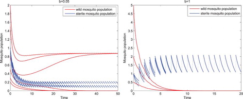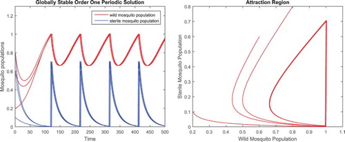1) ) has two steady states coexisting, the wild-mosquito-eradication period solution where the wild mosquito population goes to extinction, and a positive period solution where the wild mosquito population oscillates positively with almost zero amplitude and the sterile mosquito population oscillates positively and periodically as shown in the left figure in Figure 1. With $b=1>b_g$, there exists a globally asymptotically stable wild-mosquito-eradication period solution as shown in the right figure in Figure 1.

Figure 1. Parameters are given in Equation (17(17) $a=0.55,{\mu }_1=0.2,{\xi }_1=0.3,{\mu }_2=0.2,{\xi }_2=0.3,$(17) ).With $b=0.05<b_g$, system (1(1) $\begin{array}{r}\left\{\begin{array}{l}\left.\begin{array}{cc}& \frac{\mathrm{d}w\left(t\right)}{\mathrm{d}t}=w\left(\frac{aw}{w+g}-{\mu }_1-{\xi }_1(w+g)\right),\\ & \frac{\mathrm{d}g\left(t\right)}{\mathrm{d}t}=-g({\mu }_2+{\xi }_2(w+g\left)\right),\end{array}\right\}t\ne k\tau \\ \left.\begin{array}{c}w\left(t^{+}\right)=w\left(t\right),\\ g\left(t^{+}\right)=g\left(t\right)+b,\end{array}\right\}t=k\tau ,\end{array}\right.\end{array}$(1) ) has two period solutions coexisting. For the positive period solution, the wild mosquito population oscillates positively with almost zero amplitude and the sterile mosquito population oscillates positively and periodically. For the wild-mosquito-eradication period solution, the wild mosquito population goes to extinction as shown in the left figure. With $b=1>b_g$, there exists a globally asymptotically stable wild-mosquito-eradication period solution where the wild mosquito population always goes to extinction as shown in the right figure.

We next keep the same parameters but fix b=1, then ${\tau }_g=\mathrm{1.2157.}$ We then vary τ. With ether $\tau =10>{\tau }_g$ or $\tau =30>{\tau }_g$, there exists a locally asymptotically stable positive coexistence period solution for system (1(1) $\begin{array}{r}\left\{\begin{array}{l}\left.\begin{array}{cc}& \frac{\mathrm{d}w\left(t\right)}{\mathrm{d}t}=w\left(\frac{aw}{w+g}-{\mu }_1-{\xi }_1(w+g)\right),\\ & \frac{\mathrm{d}g\left(t\right)}{\mathrm{d}t}=-g({\mu }_2+{\xi }_2(w+g\left)\right),\end{array}\right\}t\ne k\tau \\ \left.\begin{array}{c}w\left(t^{+}\right)=w\left(t\right),\\ g\left(t^{+}\right)=g\left(t\right)+b,\end{array}\right\}t=k\tau ,\end{array}\right.\end{array}$(1) ) where both the wild and sterile mosquito populations oscillate. In addition, there also exists a locally asymptotically stable wild-mosquito-eradication period solution where the wild mosquito population goes to extinction as shown in the upper four figures in Figure 2. Notice that while the wild-mosquito-eradication period solution is only locally asymptotically stable and there exist positive periodic solutions for both $\tau =30$ and $\tau =10$, as the impulsive release period is shorter; that is, the sterile mosquitoes are released more often, the maximum value of the sustained oscillating wild mosquitoes becomes smaller.

Figure 2. With the same parameters given in Equation (17(17) $a=0.55,{\mu }_1=0.2,{\xi }_1=0.3,{\mu }_2=0.2,{\xi }_2=0.3,$(17) ) except b fixed, when $\tau =10$ or $\tau =30$, system (1(1) $\begin{array}{r}\left\{\begin{array}{l}\left.\begin{array}{cc}& \frac{\mathrm{d}w\left(t\right)}{\mathrm{d}t}=w\left(\frac{aw}{w+g}-{\mu }_1-{\xi }_1(w+g)\right),\\ & \frac{\mathrm{d}g\left(t\right)}{\mathrm{d}t}=-g({\mu }_2+{\xi }_2(w+g\left)\right),\end{array}\right\}t\ne k\tau \\ \left.\begin{array}{c}w\left(t^{+}\right)=w\left(t\right),\\ g\left(t^{+}\right)=g\left(t\right)+b,\end{array}\right\}t=k\tau ,\end{array}\right.\end{array}$(1) ) has a locally asymptotically stable positive coexistence period solution as shown in the upper four figures. The maximum value of the sustained oscillating wild mosquitoes for the shorter impulsive release period $\tau =10$ is smaller, as shown in the two top figures than that for the longer impulsive release period $\tau =30$ as shown in the two middle figures. With $\tau =0.9$ or $\tau =0.2$, both less than ${\tau }_g$, there exists a globally asymptotically stable wild-mosquito-eradication period solution, for system (1(1) $\begin{array}{r}\left\{\begin{array}{l}\left.\begin{array}{cc}& \frac{\mathrm{d}w\left(t\right)}{\mathrm{d}t}=w\left(\frac{aw}{w+g}-{\mu }_1-{\xi }_1(w+g)\right),\\ & \frac{\mathrm{d}g\left(t\right)}{\mathrm{d}t}=-g({\mu }_2+{\xi }_2(w+g\left)\right),\end{array}\right\}t\ne k\tau \\ \left.\begin{array}{c}w\left(t^{+}\right)=w\left(t\right),\\ g\left(t^{+}\right)=g\left(t\right)+b,\end{array}\right\}t=k\tau ,\end{array}\right.\end{array}$(1) ), where the wild mosquito population goes to extinction, as shown in the two bottom figures.

For $\tau =0.9<{\tau }_g$ or $\tau =0.2<{\tau }_g$, system (1(1) $\begin{array}{r}\left\{\begin{array}{l}\left.\begin{array}{cc}& \frac{\mathrm{d}w\left(t\right)}{\mathrm{d}t}=w\left(\frac{aw}{w+g}-{\mu }_1-{\xi }_1(w+g)\right),\\ & \frac{\mathrm{d}g\left(t\right)}{\mathrm{d}t}=-g({\mu }_2+{\xi }_2(w+g\left)\right),\end{array}\right\}t\ne k\tau \\ \left.\begin{array}{c}w\left(t^{+}\right)=w\left(t\right),\\ g\left(t^{+}\right)=g\left(t\right)+b,\end{array}\right\}t=k\tau ,\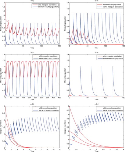end{array}\right.\end{array}$(1) ) has a globally asymptotically stable wild-mosquito-eradication period solution where the wild mosquito population goes to extinction regardless of their initial values as shown in the lower two figures in Figure 2. While the wild-mosquito-eradication period solution is globally asymptotically stable for the both cases, with the shorter impulsive release period $\tau =0.2$, or the more often releases of sterile mosquitoes, the wild mosquito population goes to extinction quicker and the maximum value of the sustained oscillating sterile mosquitoes is larger than that with the longer impulsive release period $\tau =0.9$.

We also notice that when system (1(1) $\begin{array}{r}\left\{\begin{array}{l}\left.\begin{array}{cc}& \frac{\mathrm{d}w\left(t\right)}{\mathrm{d}t}=w\left(\frac{aw}{w+g}-{\mu }_1-{\xi }_1(w+g)\right),\\ & \frac{\mathrm{d}g\left(t\right)}{\mathrm{d}t}=-g({\mu }_2+{\xi }_2(w+g\left)\right),\end{array}\right\}t\ne k\tau \\ \left.\begin{array}{c}w\left(t^{+}\right)=w\left(t\right),\\ g\left(t^{+}\right)=g\left(t\right)+b,\end{array}\right\}t=k\tau ,\end{array}\right.\end{array}$(1) ) has a locally asymptotically stable positive coexistence period solution for both $b<b_g$ and $\tau >{\tau }_g$, the dynamics for fixing τ but varying b are different from those for fixing b but varying τ, where the wild mosquito population oscillates with a very small amplitude (almost zero) in the former case, whereas the wild and sterile mosquito populations both oscillate periodically in the latter case.

4. Analysis of model (2) for the state feedback impulsive releases of sterile mosquitoes

In this section, we study the dynamics of system (2(2) $\left\{\begin{array}{l}\left.\begin{array}{cc}& \frac{\mathrm{d}w\left(t\right)}{\mathrm{d}t}=w\left(\frac{aw}{w+g}-{\mu }_1-{\xi }_1(w+g)\right),\\ & \frac{\mathrm{d}g\left(t\right)}{\mathrm{d}t}=-g({\mu }_2+{\xi }_2(w+g\left)\right),\end{array}\right\}w<w_1\text{or}\{w=w_1\text{and}g>g_1\},\\ \left.\begin{array}{c}w\left(t^{+}\right)=w\left(t\right),\\ g\left(t^{+}\right)=g\left(t\right)+b,\end{array}\right\}w=w_1\text{and}g\le g_1,\end{array}\right.$(2) ) and investigate the existence of periodic solutions and determine the attraction region of the system. Before that, we consider the qualitative features of system (2(2) $\left\{\begin{array}{l}\left.\begin{array}{cc}& \frac{\mathrm{d}w\left(t\right)}{\mathrm{d}t}=w\left(\frac{aw}{w+g}-{\mu }_1-{\xi }_1(w+g)\right),\\ & \frac{\mathrm{d}g\left(t\right)}{\mathrm{d}t}=-g({\mu }_2+{\xi }_2(w+g\left)\right),\end{array}\right\}w<w_1\text{or}\{w=w_1\text{and}g>g_1\},\\ \left.\begin{array}{c}w\left(t^{+}\right)=w\left(t\right),\\ g\left(t^{+}\right)=g\left(t\right)+b,\end{array}\right\}w=w_1\text{and}g\le g_1,\end{array}\right.$(2) ) without impulsive effects which can be written as (18) $\begin{array}{rl}& \frac{\mathrm{d}w\left(t\right)}{\mathrm{d}t}=w\left(\frac{aw}{w+g}-{\mu }_1-{\xi }_1(w+g)\right),\\ & \frac{\mathrm{d}g\left(t\right)}{\mathrm{d}t}=-g({\mu }_2+{\xi }_2(w+g\left)\right).\end{array}$(18) Clearly, system (18(18) $\begin{array}{rl}& \frac{\mathrm{d}w\left(t\right)}{\mathrm{d}t}=w\left(\frac{aw}{w+g}-{\mu }_1-{\xi }_1(w+g)\right),\\ & \frac{\mathrm{d}g\left(t\right)}{\mathrm{d}t}=-g({\mu }_2+{\xi }_2(w+g\left)\right).\end{array}$(18) ) has a globally asymptotically stable node $E(w_0,0)$, where $w_0=(a-{\mu }_1)/{\xi }_1$. In the absence of impulsive releases of sterile mosquitoes, wild mosquitoes persist and approach $w_0$, and sterile mosquitoes go extinct.

As stated in Section 2, $w_1$ is an adjustable constant threshold value for the wild mosquito density which determines what control measures should be implemented to prevent the wild mosquito density from increasing. If $w_1\ge (a-{\mu }_1)/{\xi }_1$, some other quick-acting measure (such as spraying insecticides) is required to bring the wild mosquito density down in a short time. We assume that $w_1<w_0$ throughout this section and focus our study in the region $W=\left\{\right(w,g)|0<w\le w_1,0<g<\mathrm{\infty }\}.$

4.1. Preliminary

To explore the dynamics of system (2(2) $\left\{\begin{array}{l}\left.\begin{array}{cc}& \frac{\mathrm{d}w\left(t\right)}{\mathrm{d}t}=w\left(\frac{aw}{w+g}-{\mu }_1-{\xi }_1(w+g)\right),\\ & \frac{\mathrm{d}g\left(t\right)}{\mathrm{d}t}=-g({\mu }_2+{\xi }_2(w+g\left)\right),\end{array}\right\}w<w_1\text{or}\{w=w_1\text{and}g>g_1\},\\ \left.\begin{array}{c}w\left(t^{+}\right)=w\left(t\right),\\ g\left(t^{+}\right)=g\left(t\right)+b,\end{array}\right\}w=w_1\text{and}g\le g_1,\end{array}\right.$(2) ), we firstly define two point sets $M:=\left\{\right(w,g)|w=w_1\text{and}g\le g_1\},N=\left\{\right(w,g)|w=w_1\text{and}{g}_1<g\le g_1+b\}$ which are called the impulse set and the phase set of system (2(2) $\left\{\begin{array}{l}\left.\begin{array}{cc}& \frac{\mathrm{d}w\left(t\right)}{\mathrm{d}t}=w\left(\frac{aw}{w+g}-{\mu }_1-{\xi }_1(w+g)\right),\\ & \frac{\mathrm{d}g\left(t\right)}{\mathrm{d}t}=-g({\mu }_2+{\xi }_2(w+g\left)\right),\end{array}\right\}w<w_1\text{or}\{w=w_1\text{and}g>g_1\},\\ \left.\begin{array}{c}w\left(t^{+}\right)=w\left(t\right),\\ g\left(t^{+}\right)=g\left(t\right)+b,\end{array}\right\}w=w_1\text{and}g\le g_1,\end{array}\right.$(2) ), respectively.

In the following, we construct a Poincaré map and give the definitions of successor function and order k periodic solution.

Suppose that the trajectory of system (2(2) $\left\{\begin{array}{l}\left.\begin{array}{cc}& \frac{\mathrm{d}w\left(t\right)}{\mathrm{d}t}=w\left(\frac{aw}{w+g}-{\mu }_1-{\xi }_1(w+g)\right),\\ & \frac{\mathrm{d}g\left(t\right)}{\mathrm{d}t}=-g({\mu }_2+{\xi }_2(w+g\left)\right),\end{array}\right\}w<w_1\text{or}\{w=w_1\text{and}g>g_1\},\\ \left.\begin{array}{c}w\left(t^{+}\right)=w\left(t\right),\\ g\left(t^{+}\right)=g\left(t\right)+b,\end{array}\right\}w=w_1\text{and}g\le g_1,\end{array}\right.$(2) ) starting from the point $A(w_1,g_A)$ on N firstly intersects M at point $A^{\prime }(w_1,g_{A^{\prime }})$. After the impulsive effect, it jumps to N at point $A_1(w_1,g_{A_1})$. Repeating the process above, we can get a impulsive sequence $\left\{A_k\right(w_1,g_{A_k}\left)\right\}$. Then the associated Poincaré map defined on N is given by ${\displaystyle P:N\to N,A(w_1,g_A)\to A_1(w_1,g_{A_1})}$.

Definition 4.1

[9]

We call $A_k$ the order k successor point of A, $F_1\left(A\right)=g_{A_1}-g_A$ the order one successor function of point A and $F_k\left(A\right)=g_{A_k}-g_A$ the order k successor function of point A.

Definition 4.2

[9]

A solution $\left(w\right(t),g(t\left)\right)$ of system (2(2) $\left\{\begin{array}{l}\left.\begin{array}{cc}& \frac{\mathrm{d}w\left(t\right)}{\mathrm{d}t}=w\left(\frac{aw}{w+g}-{\mu }_1-{\xi }_1(w+g)\right),\\ & \frac{\mathrm{d}g\left(t\right)}{\mathrm{d}t}=-g({\mu }_2+{\xi }_2(w+g\left)\right),\end{array}\right\}w<w_1\text{or}\{w=w_1\text{and}g>g_1\},\\ \left.\begin{array}{c}w\left(t^{+}\right)=w\left(t\right),\\ g\left(t^{+}\right)=g\left(t\right)+b,\end{array}\right\}w=w_1\text{and}g\le g_1,\end{array}\right.$(2) ) through point$A(w_1,g_A)$ at t=0 is said to be order k periodic if $g_{A_k}=g_A$.

Remark 4.1

If $F_1\left(A\right)=0,A\in N$, then system (2(2) $\left\{\begin{array}{l}\left.\begin{array}{cc}& \frac{\mathrm{d}w\left(t\right)}{\mathrm{d}t}=w\left(\frac{aw}{w+g}-{\mu }_1-{\xi }_1(w+g)\right),\\ & \frac{\mathrm{d}g\left(t\right)}{\mathrm{d}t}=-g({\mu }_2+{\xi }_2(w+g\left)\right),\end{array}\right\}w<w_1\text{or}\{w=w_1\text{and}g>g_1\},\\ \left.\begin{array}{c}w\left(t^{+}\right)=w\left(t\right),\\ g\left(t^{+}\right)=g\left(t\right)+b,\end{array}\right\}w=w_1\text{and}g\le g_1,\end{array}\right.$(2) ) has an order one periodic solution passing through point A.

Lemma 4.1

[9]

The successor function $F_1\left(A\right)$ is continuous on N.

Lemma 4.2

[9]

If there are two points $A\in N,B\in N$ such that $F_1\left(A\right)F_1\left(B\right)<0,$ then there exists a point $C\in N$ between A and B such that $F_1\left(C\right)=0$.

4.2. Existence of order one periodic solutions

Now we study the existence of order one periodic solutions of model (2(2) $\left\{\begin{array}{l}\left.\begin{array}{cc}& \frac{\mathrm{d}w\left(t\right)}{\mathrm{d}t}=w\left(\frac{aw}{w+g}-{\mu }_1-{\xi }_1(w+g)\right),\\ & \frac{\mathrm{d}g\left(t\right)}{\mathrm{d}t}=-g({\mu }_2+{\xi }_2(w+g\left)\right),\end{array}\right\}w<w_1\text{or}\{w=w_1\text{and}g>g_1\},\\ \left.\begin{array}{c}w\left(t^{+}\right)=w\left(t\right),\\ g\left(t^{+}\right)=g\left(t\right)+b,\end{array}\right\}w=w_1\text{and}g\le g_1,\end{array}\right.$(2) ).

Theorem 4.1

Suppose $w_1<(a-{\mu }_1)/{\xi }_1$ and $b>g_1,$ where $g_1$ is given in Equation (3(3) $g_1:=\frac{-({\mu }_1+2{\xi }_1{w}_1)+\sqrt{{\mu }_1^2+4a{\xi }_1{w}_1}}{2{\xi }_1}$(3) ). Then

1. System (2(2) $\left\{\begin{array}{l}\left.\begin{array}{cc}& \frac{\mathrm{d}w\left(t\right)}{\mathrm{d}t}=w\left(\frac{aw}{w+g}-{\mu }_1-{\xi }_1(w+g)\right),\\ & \frac{\mathrm{d}g\left(t\right)}{\mathrm{d}t}=-g({\mu }_2+{\xi }_2(w+g\left)\right),\end{array}\right\}w<w_1\text{or}\{w=w_1\text{and}g>g_1\},\\ \left.\begin{array}{c}w\left(t^{+}\right)=w\left(t\right),\\ g\left(t^{+}\right)=g\left(t\right)+b,\end{array}\right\}w=w_1\text{and}g\le g_1,\end{array}\right.$(2) ) has a unique order one periodic solution in region W.

2. System (2(2) $\left\{\begin{array}{l}\left.\begin{array}{cc}& \frac{\mathrm{d}w\left(t\right)}{\mathrm{d}t}=w\left(\frac{aw}{w+g}-{\mu }_1-{\xi }_1(w+g)\right),\\ & \frac{\mathrm{d}g\left(t\right)}{\mathrm{d}t}=-g({\mu }_2+{\xi }_2(w+g\left)\right),\end{array}\right\}w<w_1\text{or}\{w=w_1\text{and}g>g_1\},\\ \left.\begin{array}{c}w\left(t^{+}\right)=w\left(t\right),\\ g\left(t^{+}\right)=g\left(t\right)+b,\end{array}\right\}w=w_1\text{and}g\le g_1,\end{array}\right.$(2) ) has an attraction region in W.

Proof.

We first prove part $\left(A\right)$ as follows. Suppose that the isocline $aw/(w+g)-{\mu }_1-{\xi }_1(w+g)=0$ intersects the vertical line $w=w_1$ at point $C(w_1,g_1)$. For the point $D(w_1,g_D)$, where $g_D=g_1+b$, the trajectory from point D must intersect line $w=w_1$ at a point $D^{\mathrm{\prime }}(w_1,g_{D^{\mathrm{\prime }}})$, where $0<g_{D^{\mathrm{\prime }}}<g_1$. The point $D^{\mathrm{\prime }}$ is mapped to the point $D_1(w_1,g_{D_1})$ after the impulsive effect, and $g_D>g_{D_1}=g_{D^{\mathrm{\prime }}}+b>g_1$ because $g_1<b$ and $g_D=g_1+b$. Then, the trajectory through point $D_1$ must intersect line $w=w_1$ again at a point $D_1^{\mathrm{\prime }}(w_1,g_{D_1^{\mathrm{\prime }}})$, and the point $D_1^{\mathrm{\prime }}$ is mapped to the point $D_2(w_1,g_{D_2})$ after the impulsive effect, where $g_{D_2}=g_{D_1^{\mathrm{\prime }}}+b$. Since distinct trajectories do not intersect, we can easily get $0<g_{D^{\mathrm{\prime }}}<g_{D_1^{\mathrm{\prime }}}<g_1<g_{D_1}<g_{D_2}<g_D$. Moreover, since points D and $D_1$ are in the phase set, $D_1$ is the successor point of D and $D_2$ is the successor point of $D_1$, the successor function satisfies $F_1\left(D\right)=g_{D_1}-g_D<0$ and $F_1\left(D_1\right)=g_{D_2}-g_{D_1}>0$. By Lemmas 4.1 and 4.2, there is a point M between points $D_1$ and D such that $F_1\left(M\right)=0$, and hence the system (2(2) $\left\{\begin{array}{l}\left.\begin{array}{cc}& \frac{\mathrm{d}w\left(t\right)}{\mathrm{d}t}=w\left(\frac{aw}{w+g}-{\mu }_1-{\xi }_1(w+g)\right),\\ & \frac{\mathrm{d}g\left(t\right)}{\mathrm{d}t}=-g({\mu }_2+{\xi }_2(w+g\left)\right),\end{array}\right\}w<w_1\text{or}\{w=w_1\text{and}g>g_1\},\\ \left.\begin{array}{c}w\left(t^{+}\right)=w\left(t\right),\\ g\left(t^{+}\right)=g\left(t\right)+b,\end{array}\right\}w=w_1\text{and}g\le g_1,\end{array}\right.$(2) ) has an order one periodic solution passing though point M. (See the left figure in Figure 3).

Figure 3. Existence and uniqueness of an order one periodic solution of Equation (2(2) $\left\{\begin{array}{l}\left.\begin{array}{cc}& \frac{\mathrm{d}w\left(t\right)}{\mathrm{d}t}=w\left(\frac{aw}{w+g}-{\mu }_1-{\xi }_1(w+g)\right),\\ & \frac{\mathrm{d}g\left(t\right)}{\mathrm{d}t}=-g({\mu }_2+{\xi }_2(w+g\left)\right),\end{array}\right\}w<w_1\text{or}\{w=w_1\text{and}g>g_1\},\\ \left.\begin{array}{c}w\left(t^{+}\right)=w\left(t\right),\\ g\left(t^{+}\right)=g\left(t\right)+b,\end{array}\right\}w=w_1\text{and}g\le g_1,\end{array}\right.$(2) ).

In the following, we prove that the order one periodic solution is unique.

Suppose points $A_1$ and $A_2$ are arbitrary two points in the phase set, where $g_1<g_{A_1}<g_{A_2}<g_D$. The trajectories through points $A_1$ and $A_2$ must intersect the impulse set at some points $A_1^{\mathrm{\prime }}$ and $A_2^{\mathrm{\prime }}$, respectively, and $g_{D^{\mathrm{\prime }}}<g_{A_2^{\mathrm{\prime }}}<g_{A_1^{\mathrm{\prime }}}<g_1$. Then points $A_1^{\mathrm{\prime }}$ and $A_2^{\mathrm{\prime }}$ are mapped to points $B_1$ and $B_2$ in the phase set, respectively, where $g_{B_1}=g_{A_1^{\mathrm{\prime }}}+b$ and $g_{B_2}=g_{A_2^{\mathrm{\prime }}}+b$. Obviously, point $B_i$ is the successor point of $A_i$, $i=1,2,$ and the successor function satisfies $F_1\left(A_2\right)-F_1\left(A_1\right)=(g_{B_2}-g_{A_2})-(g_{B_1}-g_{A_1})=(g_{B_2}-g_{B_1})+(g_{A_1}-g_{A_2})<0$. Then $F_1\left(A\right)$ is monotone decreasing in the phase set, and thus there is only one point M such that $F_1\left(M\right)=0$. (See the right figure in Figure 3.)

We next prove part $\left(B\right)$. System (2(2) $\left\{\begin{array}{l}\left.\begin{array}{cc}& \frac{\mathrm{d}w\left(t\right)}{\mathrm{d}t}=w\left(\frac{aw}{w+g}-{\mu }_1-{\xi }_1(w+g)\right),\\ & \frac{\mathrm{d}g\left(t\right)}{\mathrm{d}t}=-g({\mu }_2+{\xi }_2(w+g\left)\right),\end{array}\right\}w<w_1\text{or}\{w=w_1\text{and}g>g_1\},\\ \left.\begin{array}{c}w\left(t^{+}\right)=w\left(t\right),\\ g\left(t^{+}\right)=g\left(t\right)+b,\end{array}\right\}w=w_1\text{and}g\le g_1,\end{array}\right.$(2) ) has a unique order one periodic solution passing though the point $M(w_1,g_M)$ as shown in $\left(A\right)$. Denoting the impulse point of M by $M^{\prime }$, we have $g_{M^{\prime }}<g_1<g_M=g_{M^{\prime }}+b<g_D$ where D is defined in part $\left(A\right)$.

For the successor point $D_1$ of point D, we have $g_1<g_{D_1}<g_M$. Suppose that the trajectory through point $D_1$ intersects the impulse set again at a point $D_1^{\mathrm{\prime }}$. Then point $D_1^{\mathrm{\prime }}$ is mapped to a point $D_2$ in the phase set. Since distinct trajectories do not intersect, we have $g_{D^{\mathrm{\prime }}}<g_{M^{\prime }}<g_{D_1^{\mathrm{\prime }}}<g_1$ and $g_M<g_{D_2}<g_D$.

Similarly, the trajectory from point $D_2$ intersects the impulse set again at a point $D_2^{\mathrm{\prime }}$, and then the point $D_2^{\mathrm{\prime }}$ is mapped to a point $D_3$. Thus we have $g_{D^{\mathrm{\prime }}}<g_{D_2^{\mathrm{\prime }}}<g_{M^{\prime }}$ and $g_{D_1}<g_{D_3}<g_M$.

Repeat the above steps, the trajectory from point D will underdo the impulsive effect infinitely times. Suppose that the phase point corresponding to the ith impulsive effect is $D_i$, $i=1,2,\dots$. Then we have $g_1<g_{D_1}<g_{D_3}<g_{D_5}<\cdots <g_{D_{2k+1}}<g_{D_{2(k+1)+1}}<\cdots <g_M,$ and $g_D>g_{D_2}>g_{D_4}>g_{D_6}>\cdots >g_{D_{2k}}>g_{D_{2(k+1)}}>\cdots >g_M.$ Obviously, sequences $\left\{g_{D_{2k+1}}\right\}$ and $\left\{g_{D_{2k}}\right\}$, $k=0,1,2,\dots$, are monotonically increasing and decreasing, respectively. (See Figure  4.) We further suppose $g_{D_{2k+1}}\to g_{M_1}\le g_M,\text{as}k\to \mathrm{\infty };\text{and}{g}_{D_{2k}}\to g_{M_0}\ge g_M,\text{as}k\to \mathrm{\infty },$ where the point $M_1$ may coincide with point $M_0$. Then the three points $M_1$, $M_0$, and M are the same point.

Figure 4. Illustration of the attraction region of the system (2(2) $\left\{\begin{array}{l}\left.\begin{array}{cc}& \frac{\mathrm{d}w\left(t\right)}{\mathrm{d}t}=w\left(\frac{aw}{w+g}-{\mu }_1-{\xi }_1(w+g)\right),\\ & \frac{\mathrm{d}g\left(t\right)}{\mathrm{d}t}=-g({\mu }_2+{\xi }_2(w+g\left)\right),\end{array}\right\}w<w_1\text{or}\{w=w_1\text{and}g>g_1\},\\ \left.\begin{array}{c}w\left(t^{+}\right)=w\left(t\right),\\ g\left(t^{+}\right)=g\left(t\right)+b,\end{array}\right\}w=w_1\text{and}g\le g_1,\end{array}\right.$(2) ).

Denote the impulse points of points $M_1$ and $M_0$ by $M_1^{\mathrm{\prime }}$ and $M_0^{\mathrm{\prime }}$, respectively. We can easily see that the region ${\mathrm{\Omega }}_0$ which is encircled by the closed curve $\overline{M_1{M}_0}\cup \widehat{M_0{M}_0^{\mathrm{\prime }}}\cup \overline{M_0^{\mathrm{\prime }}{M}_1^{\mathrm{\prime }}}\cup \widehat{M_1{M}_1^{\mathrm{\prime }}}$ is an invariant set. If the point $M_1$ coincides with point $M_0$, the invariant set ${\mathrm{\Omega }}_0$ is exactly the unique order one cycle $\widehat{M{M}^{\mathrm{\prime }}}\cup \overline{M^{\prime }M}$.

For any point $A_0\in \overline{D_1{M}_1}$ that is different from $M_1$, there must exist an integer k such that $g_{D_{2k+1}}<g_{A_0}<g_{D_{2(k+1)+1}}$. It is similar to the above discussion that the trajectory from point $A_0$ will also hit the impulse set infinitely times. Denoting the phase point corresponding to the lth impulsive effect by $A_l$, $l=0,1,2,\dots$, we then have $g_{D_{2(k+l+1)}^{\mathrm{\prime }}}<g_{A_{2l+1}}<g_{D_{2(k+l)}^{\mathrm{\prime }}}$ and $g_{D_{(2k+l)+1}}<g_{A_{2l}}<g_{D_{2(k+l+1)+1}^{\mathrm{\prime }}}$. Thus sequences $\left\{g_{A_{2l+1}}\right\}$ and $\left\{g_{A_{2l}}\right\}$, $l=0,1,2,\dots$, are also monotonically increasing and decreasing, respectively, and $g_{A_{2l+1}}\to g_{M_1},l\to \mathrm{\infty };\text{and}{g}_{A_{2l}}\to g_{M_0},l\to \mathrm{\infty }.$ Then the trajectory from $A_0$ is eventually attracted to the region ${\mathrm{\Omega }}_0$.

Similarly, we can show that the trajectory from point $A_0\in \overline{M_{0}D}$ also tends to the region ${\mathrm{\Omega }}_0$. Hence ${\mathrm{\Omega }}_0$ is the attraction region of system (2(2) $\left\{\begin{array}{l}\left.\begin{array}{cc}& \frac{\mathrm{d}w\left(t\right)}{\mathrm{d}t}=w\left(\frac{aw}{w+g}-{\mu }_1-{\xi }_1(w+g)\right),\\ & \frac{\mathrm{d}g\left(t\right)}{\mathrm{d}t}=-g({\mu }_2+{\xi }_2(w+g\left)\right),\end{array}\right\}w<w_1\text{or}\{w=w_1\text{and}g>g_1\},\\ \left.\begin{array}{c}w\left(t^{+}\right)=w\left(t\right),\\ g\left(t^{+}\right)=g\left(t\right)+b,\end{array}\right\}w=w_1\text{and}g\le g_1,\end{array}\right.$(2) ) in the region encircled by the closed curve $\overline{D_{1}D}\cup \widehat{D{D}^{\mathrm{\prime }}}\cup \overline{D^{\mathrm{\prime }}{D}_1^{\mathrm{\prime }}}\cup \widehat{D_1{D}_1^{\mathrm{\prime }}}$ (see Figure 4).

Besides, for any point $A\in W$, the trajectory from point A must pass through the segment $\overline{D_{1}D}$ after undergoing several times of the impulsive effect, and then tend to the region ${\mathrm{\Omega }}_0$. Thus the region ${\mathrm{\Omega }}_0$ is the attraction region of the system (2(2) $\left\{\begin{array}{l}\left.\begin{array}{cc}& \frac{\mathrm{d}w\left(t\right)}{\mathrm{d}t}=w\left(\frac{aw}{w+g}-{\mu }_1-{\xi }_1(w+g)\right),\\ & \frac{\mathrm{d}g\left(t\right)}{\mathrm{d}t}=-g({\mu }_2+{\xi }_2(w+g\left)\right),\end{array}\right\}w<w_1\text{or}\{w=w_1\text{and}g>g_1\},\\ \left.\begin{array}{c}w\left(t^{+}\right)=w\left(t\right),\\ g\left(t^{+}\right)=g\left(t\right)+b,\end{array}\right\}w=w_1\text{and}g\le g_1,\end{array}\right.$(2) ) in the region W.

The proof is completed.

Remark 4.2

If the invariant set ${\mathrm{\Omega }}_0$ is exactly the unique order one cycle $\widehat{M{M}^{\mathrm{\prime }}}\cup \overline{M^{\prime }M}$, then the order one cycle is the attractor and is globally orbitally asymptotically stable in W.

We give an example to demonstrate the results of Theorem 4.1 as follows.

Example 4.1

Given parameters (19) $a=0.55,{\mu }_1=0.2,{\xi }_1=0.3,{\mu }_2=0.2,{\xi }_2=0.3,$(19) we set the adjustable constant threshold value of wild mosquito density $w_1=1$. Then $w_1<(a-{\mu }_1)/{\xi }_1=1.16$ and $g_1=0.0611$.

For $b=0.7>g_1$, there exists a globally asymptotically stable positive order one periodic solution as shown in the left figure in Figure 5, and an attraction region in W as shown in the right figure in Figure 5.

Figure 5. Parameters are given in Equation (19(19) $a=0.55,{\mu }_1=0.2,{\xi }_1=0.3,{\mu }_2=0.2,{\xi }_2=0.3,$(19) ). The conditions in Theorem 4.1 are satisfied. There exists a positive order one periodic solution and the solutions with initial values $w\left(0\right)=0.2,0.6,0.8$, respectively, clearly approach it as shown in the left figure, and there exists an attraction region in W for system (2(2) $\left\{\begin{array}{l}\left.\begin{array}{cc}& \frac{\mathrm{d}w\left(t\right)}{\mathrm{d}t}=w\left(\frac{aw}{w+g}-{\mu }_1-{\xi }_1(w+g)\right),\\ & \frac{\mathrm{d}g\left(t\right)}{\mathrm{d}t}=-g({\mu }_2+{\xi }_2(w+g\left)\right),\end{array}\right\}w<w_1\text{or}\{w=w_1\text{and}g>g_1\},\\ \left.\begin{array}{c}w\left(t^{+}\right)=w\left(t\right),\\ g\left(t^{+}\right)=g\left(t\right)+b,\end{array}\right\}w=w_1\text{and}g\le g_1,\end{array}\right.$(2) ) as shown in the right figure.

4.3. Wild mosquitoes control

The strategies to control wild mosquitoes in system (2(2) $\left\{\begin{array}{l}\left.\begin{array}{cc}& \frac{\mathrm{d}w\left(t\right)}{\mathrm{d}t}=w\left(\frac{aw}{w+g}-{\mu }_1-{\xi }_1(w+g)\right),\\ & \frac{\mathrm{d}g\left(t\right)}{\mathrm{d}t}=-g({\mu }_2+{\xi }_2(w+g\left)\right),\end{array}\right\}w<w_1\text{or}\{w=w_1\text{and}g>g_1\},\\ \left.\begin{array}{c}w\left(t^{+}\right)=w\left(t\right),\\ g\left(t^{+}\right)=g\left(t\right)+b,\end{array}\right\}w=w_1\text{and}g\le g_1,\end{array}\right.$(2) ) are different from those in system (1(1) $\begin{array}{r}\left\{\begin{array}{l}\left.\begin{array}{cc}& \frac{\mathrm{d}w\left(t\right)}{\mathrm{d}t}=w\left(\frac{aw}{w+g}-{\mu }_1-{\xi }_1(w+g)\right),\\ & \frac{\mathrm{d}g\left(t\right)}{\mathrm{d}t}=-g({\mu }_2+{\xi }_2(w+g\left)\right),\end{array}\right\}t\ne k\tau \\ \left.\begin{array}{c}w\left(t^{+}\right)=w\left(t\right),\\ g\left(t^{+}\right)=g\left(t\right)+b,\end{array}\right\}t=k\tau ,\end{array}\right.\end{array}$(1) ). There are two control measures based on the two thresholds $w_1$ and $g_1$, in addition to the release rate b. Threshold $w_1$ determines what level of the wild mosquito abundance is allowed before sterile mosquitoes are released, that is, when to release the sterile mosquitoes, whereas threshold $g_1$ determines the existing size of the sterile mosquito population smaller than that new sterile mosquitoes need to be released, that is, the frequency of the releases or how often the sterile mosquitoes are released. Threshold $g_1$ is not independent of $w_1$, but a convex function of $w_1$ which has a single maximum value at the critical point (20) ${\overline{w}}_1:=\frac{a^2-{\mu }_1^2}{4a{\xi }_1},$(20) such that $g_1^{\prime }\left(w_1\right)=\frac{4a\xi -2{\xi }_1\sqrt{{\mu }_1^2+4a{\xi }_1{w}_1}}{2{\xi }_1\sqrt{{\mu }_1^2+4a{\xi }_1{w}_1}}\left\{\begin{array}{ll}>0,& \mathrm{\forall }{w}_1<{\overline{w}}_1,\\ <0,& \mathrm{\forall }{w}_1>{\overline{w}}_1.\end{array}\right.$

Note that to have the wild mosquitoes under better control, if the level of the wild mosquito abundance is larger when the sterile mosquitoes are released, the sterile mosquitoes need to be released more often; that is, $g_1$ needs to be smaller. Thus, we assume $w_1$ satisfies (21) ${\overline{w}}_1<w_1<w_0.$(21)

The analysis for the impact of the time or frequency of sterile mosquitoes releases on the wild mosquitoes control seems mathematically untractable because we have been unable to find an analytic formula for the solutions or the order one periodic solution for system (2(2) $\left\{\begin{array}{l}\left.\begin{array}{cc}& \frac{\mathrm{d}w\left(t\right)}{\mathrm{d}t}=w\left(\frac{aw}{w+g}-{\mu }_1-{\xi }_1(w+g)\right),\\ & \frac{\mathrm{d}g\left(t\right)}{\mathrm{d}t}=-g({\mu }_2+{\xi }_2(w+g\left)\right),\end{array}\right\}w<w_1\text{or}\{w=w_1\text{and}g>g_1\},\\ \left.\begin{array}{c}w\left(t^{+}\right)=w\left(t\right),\\ g\left(t^{+}\right)=g\left(t\right)+b,\end{array}\right\}w=w_1\text{and}g\le g_1,\end{array}\right.$(2) ). We hence provide numerical examples to illustrate the model dynamics of system with different control measures as follows.

Example 4.2

In this example, we fix $w_1$ and hence $g_1$, the time and frequency of the releases, but vary the size of the releases of the sterile mosquitoes.

The parameters are given as (22) $a=0.55,{\mu }_1=0.2,{\xi }_1=0.3,{\mu }_2=0.2,{\xi }_2=\mathrm{0.3.}$(22) Then ${\overline{w}}_1=0.3977$ and $w_0=1.1667$. We fix $w_1=1$ which is between ${\overline{w}}_1$ and $w_0$, and vary b. The initial values are $w\left(0\right)=0.9=g\left(0\right)$ for all solutions such that they are all in W.

For b=0.05 sufficiently small, the dynamics of system (2(2) $\left\{\begin{array}{l}\left.\begin{array}{cc}& \frac{\mathrm{d}w\left(t\right)}{\mathrm{d}t}=w\left(\frac{aw}{w+g}-{\mu }_1-{\xi }_1(w+g)\right),\\ & \frac{\mathrm{d}g\left(t\right)}{\mathrm{d}t}=-g({\mu }_2+{\xi }_2(w+g\left)\right),\end{array}\right\}w<w_1\text{or}\{w=w_1\text{and}g>g_1\},\\ \left.\begin{array}{c}w\left(t^{+}\right)=w\left(t\right),\\ g\left(t^{+}\right)=g\left(t\right)+b,\end{array}\right\}w=w_1\text{and}g\le g_1,\end{array}\right.$(2) ) are similar to the dynamics of system (18(18) $\begin{array}{rl}& \frac{\mathrm{d}w\left(t\right)}{\mathrm{d}t}=w\left(\frac{aw}{w+g}-{\mu }_1-{\xi }_1(w+g)\right),\\ & \frac{\mathrm{d}g\left(t\right)}{\mathrm{d}t}=-g({\mu }_2+{\xi }_2(w+g\left)\right).\end{array}$(18) ) such that there exists a globally asymptotically stable node $E(w_0,0)$. 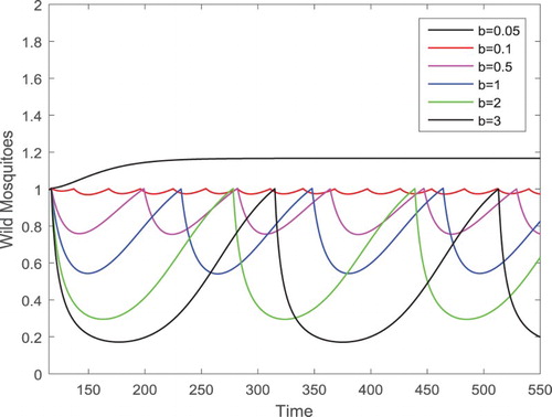We gradually increase b to b=0.1,0.5,1,2,3, respectively. Then there exist periodic solutions with a larger period and amplitude corresponding to the smaller value b as shown in Figure 6 where only the components of the wild mosquitoes are presented for a better view. We notice that the maximum values of the periodic solutions are closely equal for different b, but the minimum values of the periodic solutions are decreased as b increases which implies that the larger amount of releases of the sterile mosquitoes can drive the size of the wild mosquito population down to be smaller periodically.

Figure 6. Parameters are given in Equation (22(22) $a=0.55,{\mu }_1=0.2,{\xi }_1=0.3,{\mu }_2=0.2,{\xi }_2=\mathrm{0.3.}$(22) ). Only the components of the wild mosquitoes are presented in this figure. For the sufficiently small b=0.05, solutions approach the globally asymptotically stable unique fixed point $(w_0,0)$ that the wild mosquito component is shown as the very top curve. For b=0.1,0.5,1,2,3, respectively, corresponding periodic solutions exist as shown. The variance of the maximum values of the periodic solutions are not significant for different b, but the minimum values of the periodic solutions are clearly decreased as b increases.

Example 4.3

We show, in this example, how the dynamics change as b is fixed but $w_1$ and hence the corresponding $g_1$ both vary.

The parameters are given as (23) $a=2.5,{\mu }_1=0.2,{\xi }_1=0.3,{\mu }_2=0.2,{\xi }_2=0.3,$(23) b=10 is fixed, and the initial values $w\left(0\right)=1=g\left(0\right)$ for all solutions are also fixed.

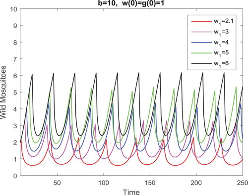
The critical point is ${\overline{w}}_1=2.07$ in this case. We then choose $w_1=2.1,3,4,5,6$, all greater than ${\overline{w}}_1$. As in Example 4.2, we only present the components of the wild mosquitoes in Figure 7. It is clear from Figure 7 that both the maximum and minimum values of the periodic solution with smaller $w_1$ and hence larger $g_1$ are smaller than those with lager $w_1$. Thus, it is better to release the sterile mosquitoes as soon as possible with the level of the wild mosquito abundance still relatively lower. If we wait until the level of the wild mosquito abundance becomes higher, even the sterile mosquitoes are released more often, both the maximum and minimum values of the oscillatory wild mosquito population become higher.

Figure 7. Parameters are given in Equation (23(23) $a=2.5,{\mu }_1=0.2,{\xi }_1=0.3,{\mu }_2=0.2,{\xi }_2=0.3,$(23) ). Only the components of the wild mosquitoes are presented in this figure. Clearly, both the maximum and minimum values of the periodic solution with smaller $w_1$ and hence larger $g_1$ are smaller than those with larger $w_1$ and hence smaller $g_1$.

5. Concluding remarks

The SIT has been applied to reduce or eradicate wild mosquitoes which transmit mosquito-borne diseases. There are many studies with various mathematical models on strategies of releases of sterile mosquitoes available in the literature and the interactive dynamics of wild and sterile mosquitoes are so complex that investigations and assessments of the impact of release strategies are challenging. We, in this paper, proposed two new strategies and formulated models (1(1) $\begin{array}{r}\left\{\begin{array}{l}\left.\begin{array}{cc}& \frac{\mathrm{d}w\left(t\right)}{\mathrm{d}t}=w\left(\frac{aw}{w+g}-{\mu }_1-{\xi }_1(w+g)\right),\\ & \frac{\mathrm{d}g\left(t\right)}{\mathrm{d}t}=-g({\mu }_2+{\xi }_2(w+g\left)\right),\end{array}\right\}t\ne k\tau \\ \left.\begin{array}{c}w\left(t^{+}\right)=w\left(t\right),\\ g\left(t^{+}\right)=g\left(t\right)+b,\end{array}\right\}t=k\tau ,\end{array}\right.\end{array}$(1) ) and (2(2) $\left\{\begin{array}{l}\left.\begin{array}{cc}& \frac{\mathrm{d}w\left(t\right)}{\mathrm{d}t}=w\left(\frac{aw}{w+g}-{\mu }_1-{\xi }_1(w+g)\right),\\ & \frac{\mathrm{d}g\left(t\right)}{\mathrm{d}t}=-g({\mu }_2+{\xi }_2(w+g\left)\right),\end{array}\right\}w<w_1\text{or}\{w=w_1\text{and}g>g_1\},\\ \left.\begin{array}{c}w\left(t^{+}\right)=w\left(t\right),\\ g\left(t^{+}\right)=g\left(t\right)+b,\end{array}\right\}w=w_1\text{and}g\le g_1,\end{array}\right.$(2) ) to describe the strategies. We built a theoretical framework to gain insights into the impact of the strategies on the control of wild mosquitoes.

In model system (1(1) $\begin{array}{r}\left\{\begin{array}{l}\left.\begin{array}{cc}& \frac{\mathrm{d}w\left(t\right)}{\mathrm{d}t}=w\left(\frac{aw}{w+g}-{\mu }_1-{\xi }_1(w+g)\right),\\ & \frac{\mathrm{d}g\left(t\right)}{\mathrm{d}t}=-g({\mu }_2+{\xi }_2(w+g\left)\right),\end{array}\right\}t\ne k\tau \\ \left.\begin{array}{c}w\left(t^{+}\right)=w\left(t\right),\\ g\left(t^{+}\right)=g\left(t\right)+b,\end{array}\right\}t=k\tau ,\end{array}\right.\end{array}$(1) ), we assume that the sterile mosquitoes are released in the fashion of periodic impulses such that the control measures are characterized by the release rate of sterile mosquitoes b and the period of impulsive releases τ. The two control measures are independent. We showed that system (1(1) $\begin{array}{r}\left\{\begin{array}{l}\left.\begin{array}{cc}& \frac{\mathrm{d}w\left(t\right)}{\mathrm{d}t}=w\left(\frac{aw}{w+g}-{\mu }_1-{\xi }_1(w+g)\right),\\ & \frac{\mathrm{d}g\left(t\right)}{\mathrm{d}t}=-g({\mu }_2+{\xi }_2(w+g\left)\right),\end{array}\right\}t\ne k\tau \\ \left.\begin{array}{c}w\left(t^{+}\right)=w\left(t\right),\\ g\left(t^{+}\right)=g\left(t\right)+b,\end{array}\right\}t=k\tau ,\end{array}\right.\end{array}$(1) ) has a unique wild-mosquito-eradication periodic solution $(0,g^{\ast }(t\left)\right)$ which is always locally asymptotically stable. An explicit formula (8(8) $g^{\ast }\left(t\right)=\frac{x_0{\mu }_2\exp (-{\mu }_2(t-k\tau \left)\right)}{{\mu }_2+{\xi }_2{x}_0(1-\exp (-{\mu }_2(t-k\tau \left)\right))},t\in (k\tau ,(k+1\left)\tau \right],$(8) ) for $g^{\ast }\left(t\right)$ is also provided. We then obtained condition (11(11) $(a-{\mu }_1{)}^2<{\xi }_1{y}^{\ast }(\tau \left)\right(a+{\xi }_1{y}^{\ast }\left(\tau \right)),$(11) ) under which the unique wild-mosquito-eradication periodic solution is globally asymptotically stable. Using the sterile mosquito release rate b and the release period τ as control measures, respectively, we derived threshold values $b_g$ and ${\tau }_g$. We first fix τ and vary b. Under condition (15(15) $(a-{\mu }_1{)}^2<\frac{{\xi }_1{M}_2}{{\xi }_2(\exp (M_2\tau )-1)}\left(a+\frac{{\xi }_1{M}_2}{{\xi }_2(\exp (M_2\tau )-1)}\right):=\overline{\alpha }.$(15) ), if b is greater than $b_g$, system (1(1) $\begin{array}{r}\left\{\begin{array}{l}\left.\begin{array}{cc}& \frac{\mathrm{d}w\left(t\right)}{\mathrm{d}t}=w\left(\frac{aw}{w+g}-{\mu }_1-{\xi }_1(w+g)\right),\\ & \frac{\mathrm{d}g\left(t\right)}{\mathrm{d}t}=-g({\mu }_2+{\xi }_2(w+g\left)\right),\end{array}\right\}t\ne k\tau \\ \left.\begin{array}{c}w\left(t^{+}\right)=w\left(t\right),\\ g\left(t^{+}\right)=g\left(t\right)+b,\end{array}\right\}t=k\tau ,\end{array}\right.\end{array}$(1) ) has a globally asymptotically stable wild-mosquito-eradication periodic solution, and if b is much less than $b_g$, the periodic solution becomes only locally asymptotically stable and other positive steady states may appear. We then fix b and vary τ. If τ is less than ${\tau }_g$, system (1(1) $\begin{array}{r}\left\{\begin{array}{l}\left.\begin{array}{cc}& \frac{\mathrm{d}w\left(t\right)}{\mathrm{d}t}=w\left(\frac{aw}{w+g}-{\mu }_1-{\xi }_1(w+g)\right),\\ & \frac{\mathrm{d}g\left(t\right)}{\mathrm{d}t}=-g({\mu }_2+{\xi }_2(w+g\left)\right),\end{array}\right\}t\ne k\tau \\ \left.\begin{array}{c}w\left(t^{+}\right)=w\left(t\right),\\ g\left(t^{+}\right)=g\left(t\right)+b,\end{array}\right\}t=k\tau ,\end{array}\right.\end{array}$(1) ) has a globally asymptotically stable wild-mosquito-eradication periodic solution. The periodic solution becomes only locally asymptotically stable if τ is much greater than ${\tau }_g$. We provided numerical simulations in Example 3.1 to illustrate these phenomena.

In either cases, sufficiently small release rate b or long impulse release period τ lead to the coexistence of both wild and sterile mosquitoes. However, as the release rate b exceeds the threshold $b_g$, or the impulse period of the releases τ is smaller than the threshold ${\tau }_g$, the releases of sterile mosquitoes drive the wild mosquito population to extinct. The dynamics of the interactive mosquitoes are shown in Figures 1 and 2, respectively.

In model system (2(2) $\left\{\begin{array}{l}\left.\begin{array}{cc}& \frac{\mathrm{d}w\left(t\right)}{\mathrm{d}t}=w\left(\frac{aw}{w+g}-{\mu }_1-{\xi }_1(w+g)\right),\\ & \frac{\mathrm{d}g\left(t\right)}{\mathrm{d}t}=-g({\mu }_2+{\xi }_2(w+g\left)\right),\end{array}\right\}w<w_1\text{or}\{w=w_1\text{and}g>g_1\},\\ \left.\begin{array}{c}w\left(t^{+}\right)=w\left(t\right),\\ g\left(t^{+}\right)=g\left(t\right)+b,\end{array}\right\}w=w_1\text{and}g\le g_1,\end{array}\right.$(2) ), we assume that, in addition to the release rate b, a constant threshold value $w_1$ for the wild mosquito density can be preadjusted and preset such that we can determine when the sterile mosquitoes will be released, characterized by $w_1$, and meanwhile how often the sterile mosquitoes will be released, characterized by $g_1$ which is correlated with $w_1$. We choose $g_1$ to be a decreasing function of $w_1$ such that $g_1$ is smaller for larger $w_1$. That is, if we allow a larger wild mosquito population when sterile mosquitoes are released, the releases need to be more frequently to have wild mosquitoes under control. Instead of possibly eradicating the wild mosquitoes, it aims at keeping the wild mosquito population down to an acceptable level. The adoption of this strategy may be due to the release affordability or special environmental situations with significant abundance of existing wild mosquitoes.

Notice that the setting of the releases of sterile mosquitoes in model (2(2) $\left\{\begin{array}{l}\left.\begin{array}{cc}& \frac{\mathrm{d}w\left(t\right)}{\mathrm{d}t}=w\left(\frac{aw}{w+g}-{\mu }_1-{\xi }_1(w+g)\right),\\ & \frac{\mathrm{d}g\left(t\right)}{\mathrm{d}t}=-g({\mu }_2+{\xi }_2(w+g\left)\right),\end{array}\right\}w<w_1\text{or}\{w=w_1\text{and}g>g_1\},\\ \left.\begin{array}{c}w\left(t^{+}\right)=w\left(t\right),\\ g\left(t^{+}\right)=g\left(t\right)+b,\end{array}\right\}w=w_1\text{and}g\le g_1,\end{array}\right.$(2) ) is based on the level of the existing wild mosquito abundance which is different from model (1(1) $\begin{array}{r}\left\{\begin{array}{l}\left.\begin{array}{cc}& \frac{\mathrm{d}w\left(t\right)}{\mathrm{d}t}=w\left(\frac{aw}{w+g}-{\mu }_1-{\xi }_1(w+g)\right),\\ & \frac{\mathrm{d}g\left(t\right)}{\mathrm{d}t}=-g({\mu }_2+{\xi }_2(w+g\left)\right),\end{array}\right\}t\ne k\tau \\ \left.\begin{array}{c}w\left(t^{+}\right)=w\left(t\right),\\ g\left(t^{+}\right)=g\left(t\right)+b,\end{array}\right\}t=k\tau ,\end{array}\right.\end{array}$(1) ) where sterile mosquitoes are released at regular time τ. The wild-mosquito-eradication periodic solution no longer exists in (2(2) $\left\{\begin{array}{l}\left.\begin{array}{cc}& \frac{\mathrm{d}w\left(t\right)}{\mathrm{d}t}=w\left(\frac{aw}{w+g}-{\mu }_1-{\xi }_1(w+g)\right),\\ & \frac{\mathrm{d}g\left(t\right)}{\mathrm{d}t}=-g({\mu }_2+{\xi }_2(w+g\left)\right),\end{array}\right\}w<w_1\text{or}\{w=w_1\text{and}g>g_1\},\\ \left.\begin{array}{c}w\left(t^{+}\right)=w\left(t\right),\\ g\left(t^{+}\right)=g\left(t\right)+b,\end{array}\right\}w=w_1\text{and}g\le g_1,\end{array}\right.$(2) ), and the sterile mosquitoes can go distinct with sufficiently small b. Furthermore, we established conditions under which system (2(2) $\left\{\begin{array}{l}\left.\begin{array}{cc}& \frac{\mathrm{d}w\left(t\right)}{\mathrm{d}t}=w\left(\frac{aw}{w+g}-{\mu }_1-{\xi }_1(w+g)\right),\\ & \frac{\mathrm{d}g\left(t\right)}{\mathrm{d}t}=-g({\mu }_2+{\xi }_2(w+g\left)\right),\end{array}\right\}w<w_1\text{or}\{w=w_1\text{and}g>g_1\},\\ \left.\begin{array}{c}w\left(t^{+}\right)=w\left(t\right),\\ g\left(t^{+}\right)=g\left(t\right)+b,\end{array}\right\}w=w_1\text{and}g\le g_1,\end{array}\right.$(2) ) has a unique order one periodic solution and an attraction region in W. Using numerical examples, we illustrated how we can have the interacting mosquitoes under control by selecting the control measures accordingly. While wild mosquitoes cannot be completely wiped out, with fixed $w_1$, increasing the release rate b can drive the minimum value of the periodically oscillatory wild mosquito population closer to zero shown in Example 4.2. On the other hand, with fixed b, we showed, in Example 4.3, that releasing the sterile mosquitoes as soon as possible with the level of the wild mosquito abundance still relatively lower is more effective than waiting until the level of the wild mosquito abundance becomes larger even with higher frequency of releases then.

The dynamics of system (1(1) $\begin{array}{r}\left\{\begin{array}{l}\left.\begin{array}{cc}& \frac{\mathrm{d}w\left(t\right)}{\mathrm{d}t}=w\left(\frac{aw}{w+g}-{\mu }_1-{\xi }_1(w+g)\right),\\ & \frac{\mathrm{d}g\left(t\right)}{\mathrm{d}t}=-g({\mu }_2+{\xi }_2(w+g\left)\right),\end{array}\right\}t\ne k\tau \\ \left.\begin{array}{c}w\left(t^{+}\right)=w\left(t\right),\\ g\left(t^{+}\right)=g\left(t\right)+b,\end{array}\right\}t=k\tau ,\end{array}\right.\end{array}$(1) ) and (2(2) $\left\{\begin{array}{l}\left.\begin{array}{cc}& \frac{\mathrm{d}w\left(t\right)}{\mathrm{d}t}=w\left(\frac{aw}{w+g}-{\mu }_1-{\xi }_1(w+g)\right),\\ & \frac{\mathrm{d}g\left(t\right)}{\mathrm{d}t}=-g({\mu }_2+{\xi }_2(w+g\left)\right),\end{array}\right\}w<w_1\text{or}\{w=w_1\text{and}g>g_1\},\\ \left.\begin{array}{c}w\left(t^{+}\right)=w\left(t\right),\\ g\left(t^{+}\right)=g\left(t\right)+b,\end{array}\right\}w=w_1\text{and}g\le g_1,\end{array}\right.$(2) ) are complex. While much progress has been achieved and, in particular, the theoretical framework has been established for both model systems and presented in this paper, rigorous proofs of positive periodic solutions for both models are to be obtained, and further investigations into other possible dynamical features should also be carried out, which are in our future research projects. Moreover, other strategies of releases such as proportional to the wild mosquito population size or proportional to the wild mosquito population size but with saturation, incorporating with the periodic impulsive releases, may provide other useful strategies. Besides, several studies [11,28] have considered the spatial component in the SIT modelling for mosquitoes are assumed to move randomly in an environment. So, developing an SIT model incorporating mosquito dispersal is also important for the assessment of the impact of release strategies. These are under our future explorations.

Acknowledgments

The authors thank two anonymous reviewers for their careful reading and valuable comments and suggestions.

Disclosure statement

No potential conflict of interest was reported by the authors.

Additional information

Funding

Mingzhan Huang and Xinyu Song were partially supported by the National Natural Science Foundation of China [11671346, 11501489, 11371305, 11371306 and 11301453], Nanhu Scholars Program of XYNU, Foundation and frontier project of Henan Province [152300410019] and Project of Department of Education of Henan Province [14B110034]. Jia Li was supported partially by U.S. National Science Foundation grant [DMS-1118150].

References

- L. Alphey, M. Benedict, R. Bellini, G.G. Clark, D.A. Dame, M.W. Service, and S.L. Dobson, Sterile-insect methods for control of mosquito-borne diseases: An analysis, Vector-Borne Zoonotic Dis. 10 (2010), pp. 295–311. doi: 10.1089/vbz.2009.0014
- R. Anguelov, Y. Dumont, and J.M.S. Lubuma, Mathematical modeling of sterile insect technology for control of anopheles mosquito, Comput. Math. Appl. 64 (2012), pp. 374–389. doi: 10.1016/j.camwa.2012.02.068
- D.D. Bainov and P.S. Simeonov, Impulsive Differential Equations: Periodic Solutions and Applications, Pitman Monographs and Surveys in Pure and Applied Mathematics, Pitman, London, 1993.
- D.D. Bainov and P.S. Simeonov, System with Impulse Effect Theory and Applications, Ellis Harwood series in Mathematics and its Applications, Ellis Harwood, Chichester, 1993.
- H.J. Barclay, Pest population stability under sterile releases, Res. Popul. Ecol. 24 (1982), pp. 405–416. doi: 10.1007/BF02515585
- H.J. Barclay and M. Mackuer, The sterile insect release method for pest control: A density-dependent model, Environ. Entomol. 9 (1980), pp. 810–817. doi: 10.1093/ee/9.6.810
- A.C. Bartlett and R.T. Staten, The sterile insect release method and other genetic control strategies, in Radcliffe's IPM World Textbook, 1996. Available at http://ipmworld.umn.edu/chapters/bartlett.htm.
- L.M. Cai, S.B. Ai, and J. Li, Dynamics of mosquitoes populations with different strategies for releasing sterile mosquitoes, SIAM J. Appl. Math. 74 (2014), pp. 1786–1809. doi: 10.1137/13094102X
- L.S. Chen, Pest control and geometric theory of Semi-continuous dynamical system, J. Beihua Univ. 12 (2011), pp. 1–9.
- H. Diaz, A.A. Ramirez, A. Olarte, and C. Clavijo, A model for the control of malaria using genetically modified vectors, J. Theoret. Biol. 276 (2011), pp. 57–66. doi: 10.1016/j.jtbi.2011.01.053
- C. Dufourd and Y. Dumont, Impact of environmental factors on mosquito dispersal in the prospect of Sterile Insect Technique control, Comput. Math. Appl. 66 (2013), pp. 1695–1715. doi: 10.1016/j.camwa.2013.03.024
- Y. Dumont and J. M. Tchuenche, Mathematical studies on the sterile insect technique for the Chikungunya disease and Aedes albopictus, J. Math. Biol. 65 (2012), pp. 809–854. doi: 10.1007/s00285-011-0477-6
- V.A. Dyck, J. Hendrichs, and A.S. Robinson, Sterile Insect Technique: Principles and Practice in Area-Wide Integrated Pest Managemen, Springer, Dordrecht, 2005. ISBN: 1-4020-4050-4.
- L. Esteva and H.M. Yang, Mathematical model to assess the control of Aedes aegypti mosquitoes by the sterile insect technique, Math. Biosci. 198 (2005), pp. 132–147. doi: 10.1016/j.mbs.2005.06.004
- K.R. Fister, M.L. McCarthy, S.F. Oppenheimer, and C. Collins, Optimal control of insects through sterile insect release and habitat modification, Math. Biosci. 244 (2013), pp. 201–212. doi: 10.1016/j.mbs.2013.05.008
- J.C. Flores, A mathematical model for wild and sterile species in competition: Immigration, Phys. A. 328 (2003), pp. 214–224. doi: 10.1016/S0378-4371(03)00545-4
- M.Z. Huang, J.X. Li, X.Y. Song, and H.J. Guo, Modeling Impulsive Injections of Insulin: Towards Artificial Pancreas, SIAM J. Appl. Math. 72 (2012), pp. 1524–1548. doi: 10.1137/110860306
- V. Lakshmikantham, D. Bainov, and P. Simeonov, Theory of Impulsive Differential Equations, Vol. 6, World Scientific, Singapore, 1989.
- J. Li, Simple mathematical models for interacting wild and transgenic mosquito populations, Math. Biosci. 189 (2004), pp. 39–59. doi: 10.1016/j.mbs.2004.01.001
- J. Li, Differential equations models for interacting wild and transgenic mosquito populations, J. Biol. Dyn. 2 (2008), pp. 241–258. doi: 10.1080/17513750701779633
- J. Li, Modeling of mosquitoes with dominant or recessive transgenes and Allee effects, Math. Biosci. Eng. 7 (2010), pp. 101–123.
- J. Li, Modelling of transgenic mosquitoes and impact on malaria transmission, J. Biol. Dyn. 5 (2011), pp. 474–494. doi: 10.1080/17513758.2010.523122
- J. Li, Discrete-time models with mosquitoes carrying genetically-modified bacteria, Math. Biosci. 240 (2012), pp. 35–44. doi: 10.1016/j.mbs.2012.05.012
- J. Li and Z.L. Yuan, Modelling releases of sterile mosquitoes with different strategies, J. Biol. Dyn. 9 (2015), pp. 1–14. doi: 10.1080/17513758.2014.977971
- A. Maiti, B. Patra, and G.P. Samanta, Sterile insect release method as a control measure of insect pests: A mathematical model, J. Appl. Math. Comput. 22 (2006), pp. 71–86. doi: 10.1007/BF02832038
- M. Rafikov, L. Bevilacqua, and A.P.P. Wyse, Optimal control strategy of malaria vector using genetically modified mosquitoes, J. Theoret. Biol. 258 (2009), pp. 418–425. doi: 10.1016/j.jtbi.2008.08.006
- M. Rafikov, A.P. Wyse, and L. Bevilacqua, Controlling the interaction between wild and transgenic mosquitoes, J. Nonlinear Syst. Appl. 1 (2010), pp. 21–31.
- S. S. Seirin Lee, R.E. Baker, E.A. Gaffney, and S.M. White, Optimal barrier zones for stopping the invasion of Aedes aegypti mosquitoes via transgenic or sterile insect techniques, Theoret. Ecol. 6 (2013), pp. 427–442. doi: 10.1007/s12080-013-0178-4
- S.F. Shuai, Y.J. Li, and X.G. Chen, Summarize of common monitoring methods of mosquito vectors, J. Trop. Med. 13 (2013), pp. 1292–1296.
- R.C.A. Thome, H.M. Yang, and L. Esteva, Optimal control of Aedes aegypti mosquitoes by the sterile insect technique and insecticide, Math. Biosci. 223 (2010), pp. 12–23. doi: 10.1016/j.mbs.2009.08.009
- S.M. White, P. Rohani, and S.M. Sait, Modelling pulsed releases for sterile insect techniques: Fitness costs of sterile and transgenic males and the effects on mosquito dynamics, J. Appl. Ecol. 47 (2010), pp. 1329–1339. doi: 10.1111/j.1365-2664.2010.01880.x
- Wikipedia: Sterile Insect Technique (2013). Available at http://en.wikipedia.org/wiki/Sterileinsecttechnique.
- A.P.P. Wyse, L. Bevilacqua, and M. Rafikov, Simulating malaria model for different treatment intensities in a variable environment, Ecol. Model. 206 (2007), pp. 322–330. doi: 10.1016/j.ecolmodel.2007.03.038
- http://news.163.com/15/0802/06/B008SANU00014Q4P.html.