Homogenization techniques for population dynamics in strongly heterogeneous landscapes

ABSTRACT

An important problem in spatial ecology is to understand how population-scale patterns emerge from individual-level birth, death, and movement processes. These processes, which depend on local landscape characteristics, vary spatially and may exhibit sharp transitions through behavioural responses to habitat edges, leading to discontinuous population densities. Such systems can be modelled using reaction–diffusion equations with interface conditions that capture local behaviour at patch boundaries. In this work we develop a novel homogenization technique to approximate the large-scale dynamics of the system. We illustrate our approach, which also generalizes to multiple species, with an example of logistic growth within a periodic environment. We find that population persistence and the large-scale population carrying capacity is influenced by patch residence times that depend on patch preference, as well as movement rates in adjacent patches. The forms of the homogenized coefficients yield key theoretical insights into how large-scale dynamics arise from the small-scale features.

KEYWORDS:

• Homogenization
• spatial heterogeneity
• reaction–diffusion equations
• edge behaviour
• interface conditions

AMS CLASSIFICATION:

• 92D40
• 35K57

1. Introduction

Spatial ecology aims to explain observed spatial distribution patterns of populations and to predict their response to landscape alterations. Population-level patterns emerge from individual-level processes of movement, reproduction, and death. Such processes are influenced by local landscape features as individuals adjust their behaviour to their surroundings. Movement decisions in particular determine the extent to which local conditions affect individuals. For example, predation risk for many songbirds is higher in open fields than in dense forest cover. Accordingly, many birds tend to avoid open areas, or move through quickly [19]. A fundamental problem in theoretical ecology then is to determine the extent to which individual processes on smaller scales affect population responses on larger scales. In this paper, we present a homogenization approach to the multiscale problem of how individual behavioural responses to sharp transitions in landscape features, such as forest edges, affect population-dynamical outcomes.

We cast the spatial-temporal dynamics of a population in a reaction–diffusion model of the form (1) ${\mathrm{\partial }}_{\tau }\rho (y,\tau )={\mathrm{\partial }}_y^2\left[D\right(y\left)\rho \right(y,\tau \left)\right]+{\epsilon }^{2}f(y,\rho ),$(1) where $\rho (y,\tau )$ denotes the density of the population at time τ and location $y\in \mathbb{R}.$ Growth and death dynamics are modelled by a function f that may depend on spatial location. Movement is modelled by ‘ecological diffusion’, whereby $D\left(y\right)$ denotes the motility of individuals [24]. This formulation assumes that while individuals adjust the probability of moving, they do not bias their movement in any direction. Models of the form (1(1) ${\mathrm{\partial }}_{\tau }\rho (y,\tau )={\mathrm{\partial }}_y^2\left[D\right(y\left)\rho \right(y,\tau \left)\right]+{\epsilon }^{2}f(y,\rho ),$(1) ) have been used extensively in ecological modelling [5,10,12,22]. A typical assumption for mathematical analysis is that the coefficient functions depend smoothly on the spatial variable [15,27].

Many natural landscapes exhibit edges or interfaces with sharp transitions between different landscape features, for example between forest and grassland, or lake and shore. Many human landscape alterations create similarly sharp edges, for example at a road or a subdivision. There is a wealth of empirical studies on how individuals direct their movement to avoid or cross such edges [8,20,21]. Several authors proposed approaches for how to include interfaces and individual behaviour at interfaces into reaction–diffusion equations [1,3,12,16,23]. We follow the work by [12].

We take a landscape-ecology point of view and consider the environment to consist of patches, i.e. areas that are relatively homogeneous within but substantially different from their immediate surroundings. Accordingly, motility and population growth are spatially constant within a patch but different from outside that patch. We partition a one-dimensional landscape into intervals (‘patches’) $(y_{i-1},y_i)$, $i\in \mathbb{Z},$ and have a diffusion equation on each interval. Equation (1(1) ${\mathrm{\partial }}_{\tau }\rho (y,\tau )={\mathrm{\partial }}_y^2\left[D\right(y\left)\rho \right(y,\tau \left)\right]+{\epsilon }^{2}f(y,\rho ),$(1) ) then turns into a system of the form (2) ${\mathrm{\partial }}_{\tau }\rho =D_i{\mathrm{\partial }}_y^2\rho +{\epsilon }^2{f}_i\left(\rho \right)\mathrm{for}y\in (y_{i-1},y_i),i\in \mathbb{Z}.$(2) We need to define matching conditions that link the densities and population fluxes between adjacent patches. Conservation of individuals requires that the flux be continuous across an interface, i.e. (3) $D_{i+1}{\mathrm{\partial }}_y\rho (y_i^{+},\tau )=D_i{\mathrm{\partial }}_y\rho (y_i^{-},\tau ).$(3) Here, $y_i^{+}$ and $y_i^{-}$ denote right- and left-sided limits at $y_i$.

A careful derivation of interface conditions from a random walk model reveals that the density across an interface is, in general, not continuous [16]. Rather, we use the condition [12] (4) ${\alpha }_i^{-}{D}_{i+1}\rho (y_i^{+},\tau )={\alpha }_i^{+}{D}_i\rho (y_i^{-},\tau ),$(4) where ${\alpha }_i^{+}$ (${\alpha }_i^{-}$) is the probability that an individual at interface $y_i$ moves to the right (left) such that ${\alpha }_i^{+}\in [0,1]$, and ${\alpha }_i^{-}=1-{\alpha }_i^{+}$. The formal study of systems of the form (2(2) ${\mathrm{\partial }}_{\tau }\rho =D_i{\mathrm{\partial }}_y^2\rho +{\epsilon }^2{f}_i\left(\rho \right)\mathrm{for}y\in (y_{i-1},y_i),i\in \mathbb{Z}.$(2) ) with conditions (3(3) $D_{i+1}{\mathrm{\partial }}_y\rho (y_i^{+},\tau )=D_i{\mathrm{\partial }}_y\rho (y_i^{-},\tau ).$(3) ) and (4(4) ${\alpha }_i^{-}{D}_{i+1}\rho (y_i^{+},\tau )={\alpha }_i^{+}{D}_i\rho (y_i^{-},\tau ),$(4) ) is still in its infancy, but some qualitative results about the stability of the linear system and minimal travelling wave speeds are known, assuming that the system shows a particular translational symmetry [12,13].

A powerful tool to study the dynamics of model (1(1) ${\mathrm{\partial }}_{\tau }\rho (y,\tau )={\mathrm{\partial }}_y^2\left[D\right(y\left)\rho \right(y,\tau \left)\right]+{\epsilon }^{2}f(y,\rho ),$(1) ) is multi-scale analysis and homogenization. If one assumes that the coefficient functions vary on a small scale only, one can separate scales and introduce a small-scale variable. Applying the method of multiple scales leads to a suite of equations that are solved sequentially, and the leading order solution often provides a very good approximation to the solution of the original problem [9,15,17]. The classical results on homogenization techniques require that the solution be continuous. For example, Othmer [15] applied the method of homogenization to a model of Fickian diffusion assuming continuous population density. There are very few recent papers that deal with ecological diffusion with discontinuous densities [7,14], and these analyses are restricted to the special case of no habitat preference (${\alpha }_i^{+}={\alpha }_i^{-}$). Other authors incorporated the more general interface conditions (3(3) $D_{i+1}{\mathrm{\partial }}_y\rho (y_i^{+},\tau )=D_i{\mathrm{\partial }}_y\rho (y_i^{-},\tau ).$(3) )–(4(4) ${\alpha }_i^{-}{D}_{i+1}\rho (y_i^{+},\tau )={\alpha }_i^{+}{D}_i\rho (y_i^{-},\tau ),$(4) ), but then proceeded to scale density and space in Equations (2(2) ${\mathrm{\partial }}_{\tau }\rho =D_i{\mathrm{\partial }}_y^2\rho +{\epsilon }^2{f}_i\left(\rho \right)\mathrm{for}y\in (y_{i-1},y_i),i\in \mathbb{Z}.$(2) )–(4(4) ${\alpha }_i^{-}{D}_{i+1}\rho (y_i^{+},\tau )={\alpha }_i^{+}{D}_i\rho (y_i^{-},\tau ),$(4) ) to obtain continuous densities so that the classical techniques apply [13]. This approach is unsatisfactory and does not generalize, for example to multispecies models.

In this work, we develop the theory to homogenize equations of the form (2(2) ${\mathrm{\partial }}_{\tau }\rho =D_i{\mathrm{\partial }}_y^2\rho +{\epsilon }^2{f}_i\left(\rho \right)\mathrm{for}y\in (y_{i-1},y_i),i\in \mathbb{Z}.$(2) ) with the general interface conditions (3(3) $D_{i+1}{\mathrm{\partial }}_y\rho (y_i^{+},\tau )=D_i{\mathrm{\partial }}_y\rho (y_i^{-},\tau ).$(3) )–(4(4) ${\alpha }_i^{-}{D}_{i+1}\rho (y_i^{+},\tau )={\alpha }_i^{+}{D}_i\rho (y_i^{-},\tau ),$(4) ). We treat the special case of a periodic environment consisting of two types of alternating patches, but the theory carries over to other periodic settings. More specifically, we assume the interval $(y_{i-1},y_i)$ will represent a patch of type 1 (type 2), whenever i is odd (even). All patches of type 1 have width $\mathrm{\Delta }{y}_1$, and all patches of type 2 have width $\mathrm{\Delta }{y}_2$. We set the motility coefficients and growth functions to be (5) $D_i=\left\{\begin{array}{ll}{D}_1& \text{for }i\text{ odd},\\ D_2& \text{for }i\text{ even}.\end{array}\right.f_i\left(\rho \right)=\left\{\begin{array}{ll}{f}_1\left(\rho \right)& \text{for }i\text{ odd},\\ f_2\left(\rho \right)& \text{for }i\text{ even}.\end{array}\right.$(5) The probabilities that individuals at interfaces move to the right or left may be defined similarly, by setting ${\alpha }_i^{\pm }$ equal to ${\alpha }_1^{\pm }$ when i is odd or ${\alpha }_2^{\pm }$ when i is even. However, we assume that the probability that an individual moves towards a patch of type 1 (or type 2) is independent of whether that patch is to the right or to the left of the interface. Thus, ${\alpha }_1^{-}={\alpha }_2^{+}=\alpha$, and ${\alpha }_1^{+}={\alpha }_2^{-}=1-\alpha$, and to simplify notation at the interfaces, we set (6) $k_i=\left\{\begin{array}{ll}{k}^{-1}& \text{for }i\text{ odd},\\ k& \text{for }i\text{ even},\end{array}\right.$(6) for $k=\left(\alpha /(1-\alpha )\right)\left(D_2/D_1\right)$. Then Equation (4(4) ${\alpha }_i^{-}{D}_{i+1}\rho (y_i^{+},\tau )={\alpha }_i^{+}{D}_i\rho (y_i^{-},\tau ),$(4) ) becomes (7) $\rho (y_i^{+},\tau )=k_i\rho (y_i^{-},\tau ).$(7) We present the formal derivation of the homogenization limit for this system in the next section. In Section 3, we compare the homogenization approximation with numerical simulations of the full spatial model. We discuss ecological insights from our approach as well as future directions and application in the final section.

2. Multiple scales analysis and homogenization

It is useful to introduce fast- (small-) and slow- (large-) scale temporal and spatial variables. Models of spatio-temporal dynamics may be formulated at the fast scale (Equation (1(1) ${\mathrm{\partial }}_{\tau }\rho (y,\tau )={\mathrm{\partial }}_y^2\left[D\right(y\left)\rho \right(y,\tau \left)\right]+{\epsilon }^{2}f(y,\rho ),$(1) )), accounting for variation in movement behaviour and population dynamics arising from local environmental heterogeneity. The fast-scale models can then be ‘scaled-up’ to obtain a model in terms of the slow-scale variables. To this end, the fast-scale spatial and temporal variables are y and τ, and we introduce the corresponding slow-scale variables x and t. We impose the parabolic scaling $x=\epsilon y$ and $t={\epsilon }^2\tau$, where $\epsilon \ll 1$ is a small, dimensionless parameter that describes the separation between the fast and slow scales.

At the fast scale, the spatio-temporal dynamics are given by Equation (1(1) ${\mathrm{\partial }}_{\tau }\rho (y,\tau )={\mathrm{\partial }}_y^2\left[D\right(y\left)\rho \right(y,\tau \left)\right]+{\epsilon }^{2}f(y,\rho ),$(1) ). The scale of the environmental heterogeneity is determined by $\mathrm{\Delta }{y}_1$ and $\mathrm{\Delta }{y}_2$, both of which are assumed to be small ($O\left(\epsilon \right)$). The reaction term is scaled by ${\epsilon }^2$, reflecting the assumption that growth dynamics are very slow when we are ‘zoomed-in’ on the fast scale. Lastly, we consider the diffusion coefficient to vary only with respect to the small scale.

The goal of homogenization is to obtain an approximate model that describes the slow-scale behaviour of the system by appropriately averaging the variation in the movement and growth parameters over the fast scale. The coefficients of the resulting homogenized model are constant or only vary at the slow scale [9,15,17]. Consequently, the homogenized model is much easier to analyse analytically or numerically, and often leads to important theoretical insights about the relationship between local individual movement behaviours and variation in growth rates and large-scale population-dynamical outcomes.

Proceeding formally, we assume that ρ depends explicitly on both spatial scales x and y and on the slow temporal scale t. Treating x and y as independent induces a change in derivative, ${\mathrm{\partial }}_x\to {\epsilon }^{-1}{\mathrm{\partial }}_y+{\mathrm{\partial }}_x.$ If we assume that the motilities and the growth parameters vary only at the fast scale, then in terms of the slow-scale variables, the model (2(2) ${\mathrm{\partial }}_{\tau }\rho =D_i{\mathrm{\partial }}_y^2\rho +{\epsilon }^2{f}_i\left(\rho \right)\mathrm{for}y\in (y_{i-1},y_i),i\in \mathbb{Z}.$(2) ) and interface conditions (3(3) $D_{i+1}{\mathrm{\partial }}_y\rho (y_i^{+},\tau )=D_i{\mathrm{\partial }}_y\rho (y_i^{-},\tau ).$(3) ), (7(7) $\rho (y_i^{+},\tau )=k_i\rho (y_i^{-},\tau ).$(7) ) become (8) ${\mathrm{\partial }}_t\rho =D_i({\epsilon }^{-1}{\mathrm{\partial }}_y+{\mathrm{\partial }}_x{)}^2\rho +f_i(\rho )\text{for }y\in (y_{i-1},y_i),$(8) with (9) ${\epsilon }^{-1}{D}_{i+1}({\epsilon }^{-1}{\mathrm{\partial }}_y+{\mathrm{\partial }}_x)\rho (x,y_i^{+},t)={\epsilon }^{-1}{D}_i({\epsilon }^{-1}{\mathrm{\partial }}_y+{\mathrm{\partial }}_x)\rho (x,y_i^{-},t),$(9) and (10) ${\epsilon }^{-2}\rho (x,y_i^{+},t)={\epsilon }^{-2}{k}_i\rho (x,y_i^{-},t),$(10) for $i\in \mathbb{Z}$. Coefficients and growth functions are given by (5(5) $D_i=\left\{\begin{array}{ll}{D}_1& \text{for }i\text{ odd},\\ D_2& \text{for }i\text{ even}.\end{array}\right.f_i\left(\rho \right)=\left\{\begin{array}{ll}{f}_1\left(\rho \right)& \text{for }i\text{ odd},\\ f_2\left(\rho \right)& \text{for }i\text{ even}.\end{array}\right.$(5) ), (6(6) $k_i=\left\{\begin{array}{ll}{k}^{-1}& \text{for }i\text{ odd},\\ k& \text{for }i\text{ even},\end{array}\right.$(6) ).

In the analysis that follows, we assume that $\mathrm{\Delta }{y}_1=\mathrm{\Delta }{y}_2=\mathrm{\Delta }y$. On the other hand, if the patch widths differ, then the system (2(2) ${\mathrm{\partial }}_{\tau }\rho =D_i{\mathrm{\partial }}_y^2\rho +{\epsilon }^2{f}_i\left(\rho \right)\mathrm{for}y\in (y_{i-1},y_i),i\in \mathbb{Z}.$(2) ), (3(3) $D_{i+1}{\mathrm{\partial }}_y\rho (y_i^{+},\tau )=D_i{\mathrm{\partial }}_y\rho (y_i^{-},\tau ).$(3) ), (7(7) $\rho (y_i^{+},\tau )=k_i\rho (y_i^{-},\tau ).$(7) ), expressed in terms of the fast-scale variables, may be rescaled to obtain a fast-scale system with both patch widths equal to $\mathrm{\Delta }{y}_1$. To demonstrate this, we set $y_0=0$, and we focus on the single period $(-\mathrm{\Delta }{y}_2,\mathrm{\Delta }{y}_1]$, which includes the patch to the right (type 1) and to the left (type 2) of 0. The results are then extended periodically throughout $\mathbb{R}$. We introduce the rescaled spatial variable ξ and set $\xi =y$, for $y\in (0,\mathrm{\Delta }{y}_1)$ and $\xi =\left(\mathrm{\Delta }{y}_1/\mathrm{\Delta }{y}_2\right)y$, for $y\in (-\mathrm{\Delta }{y}_2,0)$. We also set $\omega (\xi ,t)=\rho (y,t)$ for $\xi \in (0,\mathrm{\Delta }{y}_1)$, and $\omega (\xi ,t)=\left(\mathrm{\Delta }{y}_2/\mathrm{\Delta }{y}_1\right)\rho (y,t)$ for $\xi \in (-\mathrm{\Delta }{y}_1,0)$. Then the system (2(2) ${\mathrm{\partial }}_{\tau }\rho =D_i{\mathrm{\partial }}_y^2\rho +{\epsilon }^2{f}_i\left(\rho \right)\mathrm{for}y\in (y_{i-1},y_i),i\in \mathbb{Z}.$(2) ), (3(3) $D_{i+1}{\mathrm{\partial }}_y\rho (y_i^{+},\tau )=D_i{\mathrm{\partial }}_y\rho (y_i^{-},\tau ).$(3) ), (7(7) $\rho (y_i^{+},\tau )=k_i\rho (y_i^{-},\tau ).$(7) ), becomes (11) ${\mathrm{\partial }}_{\tau }\omega (\xi ,\tau )={\tilde{D}}_i{\mathrm{\partial }}_{\xi }^2\omega (\xi ,\tau )+{\epsilon }^2{\tilde{f}}_i\left(\omega \right(\xi ,\tau \left)\right),$(11) for $\xi \in (0,\mathrm{\Delta }{y}_1)$ or for $\xi \in (-\mathrm{\Delta }{y}_1,0)$, with interface conditions (12) ${\tilde{D}}_{i+1}{\mathrm{\partial }}_{\xi }\omega ({\xi }_i^{+},\tau )={\tilde{D}}_i{\mathrm{\partial }}_{\xi }\omega ({\xi }_i^{-},\tau ),$(12) and (13) $\omega ({\xi }_i^{+},t)={\tilde{k}}_i\omega ({\xi }_i^{-},\tau ).$(13) Here, the coefficients and growth functions are given by (14) $\begin{array}{rl}{\tilde{D}}_i& =\left\{\begin{array}{ll}{\tilde{D}}_1=D_1& \text{for }i\text{ odd},\\ {\tilde{D}}_2=(\mathrm{\Delta }{y}_1/\mathrm{\Delta }{y}_2{)}^2{D}_2& \text{for }i\text{ even},\end{array}\right.\end{array}$(14) (15) $\begin{array}{rl}{\tilde{f}}_i\left(\omega \right)& =\left\{\begin{array}{ll}{\tilde{f}}_1\left(\omega \right)=f_1\left(\omega \right)& \text{for }i\text{ odd},\\ {\tilde{f}}_2\left(\omega \right)=\left(\mathrm{\Delta }{y}_2/\mathrm{\Delta }{y}_1\right)f_2\left(\right(\mathrm{\Delta }{y}_1/\mathrm{\Delta }{y}_2\left)\omega \right)& \text{for }i\text{ even},\end{array}\right.\end{array}$(15) and (16) ${\tilde{k}}_i=\left\{\begin{array}{ll}{\tilde{k}}^{-1}& \text{for }i\text{ odd},\\ \tilde{k}& \text{for }i\text{ even},\end{array}\right.$(16) where $\tilde{k}=\left(\mathrm{\Delta }{y}_1/\mathrm{\Delta }{y}_2\right)k$. Scaling up the system in (11(11) ${\mathrm{\partial }}_{\tau }\omega (\xi ,\tau )={\tilde{D}}_i{\mathrm{\partial }}_{\xi }^2\omega (\xi ,\tau )+{\epsilon }^2{\tilde{f}}_i\left(\omega \right(\xi ,\tau \left)\right),$(11) )–(13(13) $\omega ({\xi }_i^{+},t)={\tilde{k}}_i\omega ({\xi }_i^{-},\tau ).$(13) ), and treating ξ and $\zeta =\epsilon \xi$ as independent, results in a system of the form (8(8) ${\mathrm{\partial }}_t\rho =D_i({\epsilon }^{-1}{\mathrm{\partial }}_y+{\mathrm{\partial }}_x{)}^2\rho +f_i(\rho )\text{for }y\in (y_{i-1},y_i),$(8) )–(10(10) ${\epsilon }^{-2}\rho (x,y_i^{+},t)={\epsilon }^{-2}{k}_i\rho (x,y_i^{-},t),$(10) ). Thus, in our analysis below (Section 2.1) we assume equal patch widths, however we give results in Section 2.2 for the more general case of two different patch lengths.

2.1. Homogenization

Since ϵ is small, we assume a series solution of the form (17) $\rho ={\rho }_0(x,y,t)+\epsilon {\rho }_1(x,y,t)+{\epsilon }^2{\rho }_2(x,y,t)+\cdots ,$(17) where each ${\rho }_j(x,y,t)$, for $j=0,1,\dots$, is a bounded function of y. The analysis that follows applies to a large class of growth functions $f_i$ that satisfy (18) $f_i\left(\rho \right)=f_i\left({\rho }_0\right)+O\left({\epsilon }^1\right).$(18) Assuming equal patch widths, we proceed by substituting the ansatz (17(17) $\rho ={\rho }_0(x,y,t)+\epsilon {\rho }_1(x,y,t)+{\epsilon }^2{\rho }_2(x,y,t)+\cdots ,$(17) ) into the model and interface conditions (8(8) ${\mathrm{\partial }}_t\rho =D_i({\epsilon }^{-1}{\mathrm{\partial }}_y+{\mathrm{\partial }}_x{)}^2\rho +f_i(\rho )\text{for }y\in (y_{i-1},y_i),$(8) )–(10(10) ${\epsilon }^{-2}\rho (x,y_i^{+},t)={\epsilon }^{-2}{k}_i\rho (x,y_i^{-},t),$(10) ), equating terms with the same powers of ϵ, and solving the resulting equations iteratively. We seek the leading order solution, ${\rho }_0$.

2.1.1. Order ${\epsilon }^{-2}$

The equations at the largest order, $O\left({\epsilon }^{-2}\right)$ are (19) $0=D_i{\mathrm{\partial }}_y^2{\rho }_0\text{for }y\in (y_{i-1},y_i),i\in \mathbb{Z},$(19) with interface conditions (20) $D_{i+1}{\mathrm{\partial }}_y{\rho }_0(x,y_i^{+},t)=D_i{\mathrm{\partial }}_y{\rho }_0(x,y_i^{-},t),$(20) and (21) ${\rho }_0(x,y_i^{+},t)=k_i{\rho }_0(x,y_i^{-},t).$(21) To solve (19(19) $0=D_i{\mathrm{\partial }}_y^2{\rho }_0\text{for }y\in (y_{i-1},y_i),i\in \mathbb{Z},$(19) ) and find ${\rho }_0$ we define $D\left(y\right)=D_i$ for $y\in (y_{i-1},y_i)$ and investigate the integral of (19(19) $0=D_i{\mathrm{\partial }}_y^2{\rho }_0\text{for }y\in (y_{i-1},y_i),i\in \mathbb{Z},$(19) ) (22) ${\int }_0^y{\mathrm{\partial }}_y^2\left(D{\rho }_0\right)(x,s,t)\mathrm{d}s={\int }_{y_{j-1}}^y{D}_j{\mathrm{\partial }}_y^2{\rho }_0(x,s,t)\mathrm{d}s+\sum _{i=1}^{j-1}{\int }_{y_{i-1}}^{y_i}{D}_i{\mathrm{\partial }}_y^2{\rho }_0(x,s,t)\mathrm{d}s,$(22) where $y\in (y_{j-1},y_j)$ for some $j\in \mathbb{Z}$. According to (19(19) $0=D_i{\mathrm{\partial }}_y^2{\rho }_0\text{for }y\in (y_{i-1},y_i),i\in \mathbb{Z},$(19) ), the integrand in each term on the right side of (22(22) ${\int }_0^y{\mathrm{\partial }}_y^2\left(D{\rho }_0\right)(x,s,t)\mathrm{d}s={\int }_{y_{j-1}}^y{D}_j{\mathrm{\partial }}_y^2{\rho }_0(x,s,t)\mathrm{d}s+\sum _{i=1}^{j-1}{\int }_{y_{i-1}}^{y_i}{D}_i{\mathrm{\partial }}_y^2{\rho }_0(x,s,t)\mathrm{d}s,$(22) ) must vanish at all values of s. Applying this fact and integrating, we obtain (23) $\begin{array}{rl}0& =\sum _{i=1}^{j-1}{D}_i\left[{\mathrm{\partial }}_y{\rho }_0(x,y_i^{-},t)-{\mathrm{\partial }}_y{\rho }_0(x,y_{i-1}^{+},t)\right]+D_j\left[{\mathrm{\partial }}_y{\rho }_0(x,y,t)-{\mathrm{\partial }}_y{\rho }_0(x,y_{j-1}^{+},t)\right].\end{array}$(23) Here, we have assumed, without loss of generality, that j>0. Applying the continuous–flux interface condition from Equation (20(20) $D_{i+1}{\mathrm{\partial }}_y{\rho }_0(x,y_i^{+},t)=D_i{\mathrm{\partial }}_y{\rho }_0(x,y_i^{-},t),$(20) ) causes the series on the right side of (23(23) $\begin{array}{rl}0& =\sum _{i=1}^{j-1}{D}_i\left[{\mathrm{\partial }}_y{\rho }_0(x,y_i^{-},t)-{\mathrm{\partial }}_y{\rho }_0(x,y_{i-1}^{+},t)\right]+D_j\left[{\mathrm{\partial }}_y{\rho }_0(x,y,t)-{\mathrm{\partial }}_y{\rho }_0(x,y_{j-1}^{+},t)\right].\end{array}$(23) ) to telescope, collapsing down to (24) $0=D_j{\mathrm{\partial }}_y{\rho }_0(x,y,t)-D_1{\mathrm{\partial }}_y{\rho }_0(x,y_0^{+},t),$(24) and, thus, (25) ${\mathrm{\partial }}_y{\rho }_0(x,y,t)=\frac{D_1{\mathrm{\partial }}_y{\rho }_0(x,y_0^{+},t)}{D\left(y\right)}.$(25) Next, in order to apply the discontinuous–density interface condition (21(21) ${\rho }_0(x,y_i^{+},t)=k_i{\rho }_0(x,y_i^{-},t).$(21) ) we define (26) $h_i=\left\{\begin{array}{ll}1& \text{for }i\text{ odd},\\ k& \text{for }i\text{ even},\end{array}\right.$(26) and let $h\left(y\right)=h_i$ for $y\in (y_{i-1},y_i)$. We then consider the integral (27) ${\int }_0^y{\mathrm{\partial }}_y\left(h{\rho }_0\right)(x,s,t)\mathrm{d}s={\int }_{y_{j-1}}^y{h}_j{\mathrm{\partial }}_y{\rho }_0(x,s,t)\mathrm{d}s+\sum _{i=1}^{j-1}{\int }_{y_{i-1}}^{y_i}{h}_i{\mathrm{\partial }}_y{\rho }_0(x,s,t)\mathrm{d}s.$(27) Integrating each term on the right side, we obtain (28) $\begin{array}{rl}{\int }_0^y{\mathrm{\partial }}_y\left(h{\rho }_0\right)(x,s,t)\mathrm{d}s& =\sum _{i=1}^{j-1}{h}_i\left[{\rho }_0(x,y_i^{-},t)-{\rho }_0(x,y_{i-1}^{+},t)\right]\\ & +h_j\left[{\rho }_0(x,y,t)-{\rho }_0(x,y_{j-1}^{+},t)\right].\end{array}$(28) Equations (26(26) $h_i=\left\{\begin{array}{ll}1& \text{for }i\text{ odd},\\ k& \text{for }i\text{ even},\end{array}\right.$(26) ) and (21(21) ${\rho }_0(x,y_i^{+},t)=k_i{\rho }_0(x,y_i^{-},t).$(21) ) imply that the series telescopes. Thus, (29) ${\int }_0^y{\mathrm{\partial }}_y\left(h{\rho }_0\right)(x,s,t)\mathrm{d}s=h_j{\rho }_0(x,y,t)-h_1{\rho }_0(x,y_0^{+},t).$(29) Alternatively, we can multiply (25(25) ${\mathrm{\partial }}_y{\rho }_0(x,y,t)=\frac{D_1{\mathrm{\partial }}_y{\rho }_0(x,y_0^{+},t)}{D\left(y\right)}.$(25) ) by $h\left(y\right)$ and integrate, to obtain (30) ${\int }_0^y{\mathrm{\partial }}_y\left(h{\rho }_0\right)(x,s,t)\mathrm{d}s=D_1{\mathrm{\partial }}_y{\rho }_0(x,y_0^{+},t){\int }_0^y\frac{h\left(s\right)}{D\left(s\right)}\mathrm{d}s.$(30) The integral on the right side can be rewritten as (31) ${\int }_0^y\frac{h\left(s\right)}{D\left(s\right)}\mathrm{d}s=\frac{h_j}{D_j}(y-y_j)+\mathrm{\Delta }y\sum _{i=1}^{j-1}\frac{h_i}{D_i},$(31) which can be simplified to yield (32) ${\int }_0^y\frac{h\left(s\right)}{D\left(s\right)}\mathrm{d}s=\frac{y}{2}\left(\frac{1}{D_1}+\frac{k}{D_2}\right)+\frac{\mathrm{\Delta }\left(y\right)}{2}\left(\frac{1}{D_1}-\frac{k}{D_2}\right),$(32) where $\mathrm{\Delta }\left(y\right)$ is defined by (33) $\mathrm{\Delta }\left(y\right)=\left\{\begin{array}{ll}y-y_{i-1}& \text{for }i\text{ odd},\\ y_i-y& \text{for }i\text{ even},\end{array}\right.$(33) for $y\in (y_{i-1},y_i)$. Note that for all y we have $0<\mathrm{\Delta }\left(y\right)<\mathrm{\Delta }y$.

Substituting (32(32) ${\int }_0^y\frac{h\left(s\right)}{D\left(s\right)}\mathrm{d}s=\frac{y}{2}\left(\frac{1}{D_1}+\frac{k}{D_2}\right)+\frac{\mathrm{\Delta }\left(y\right)}{2}\left(\frac{1}{D_1}-\frac{k}{D_2}\right),$(32) ) into (30(30) ${\int }_0^y{\mathrm{\partial }}_y\left(h{\rho }_0\right)(x,s,t)\mathrm{d}s=D_1{\mathrm{\partial }}_y{\rho }_0(x,y_0^{+},t){\int }_0^y\frac{h\left(s\right)}{D\left(s\right)}\mathrm{d}s.$(30) ), and applying (29(29) ${\int }_0^y{\mathrm{\partial }}_y\left(h{\rho }_0\right)(x,s,t)\mathrm{d}s=h_j{\rho }_0(x,y,t)-h_1{\rho }_0(x,y_0^{+},t).$(29) ), we obtain (34) $\begin{array}{rl}{\rho }_0(x,y,t)& =\frac{D_1}{h\left(y\right)}{\mathrm{\partial }}_y{\rho }_0(x,y_0^{+},t)\left[\frac{y}{2}\left(\frac{1}{D_1}+\frac{k}{D_2}\right)+\frac{\mathrm{\Delta }\left(y\right)}{2}\left(\frac{1}{D_1}-\frac{k}{D_2}\right)\right]\\ & +\frac{h_1}{h\left(y\right)}{\rho }_0(x,y_0^{+},t).\end{array}$(34) The first term on the right-hand side of this equation is $O\left(y\right)$, so that ${\rho }_0(x,y,t)$ will only remain bounded as $y\to \mathrm{\infty }$ if ${\mathrm{\partial }}_y{\rho }_0(x,y_0^{+},t)=0$. This condition implies the following simple form for ${\rho }_0$: (35) ${\rho }_0(x,y,t)=g(x,t)/h\left(y\right),$(35) where $g(x,t)={\rho }_0(x,y_0^{+},t)$ is independent of y. So it remains to find $g(x,t)$, and we do this by studying the order ${\epsilon }^{-1}$ and ${\epsilon }^0$ equations.

2.1.2. Order ${\epsilon }^{-1}$

The equations at $O\left({\epsilon }^{-1}\right)$ are (36) $0=D_i\left[{\mathrm{\partial }}_y^2{\rho }_1+2{\mathrm{\partial }}_x{\mathrm{\partial }}_y{\rho }_0\right]\text{for }y\in (y_{i-1},y_i),i\in \mathbb{Z},$(36) with interface conditions (37) $D_{i+1}\left[{\mathrm{\partial }}_y{\rho }_1+{\mathrm{\partial }}_x{\rho }_0\right](x,y_i^{+},t)=D_i\left[{\mathrm{\partial }}_y{\rho }_1+{\mathrm{\partial }}_x{\rho }_0\right](x,y_i^{-},t),$(37) and (38) ${\rho }_1(x,y_i^{+},t)=k_i{\rho }_1(x,y_i^{-},t).$(38) Since $h\left(y\right)$ is constant over each patch $(y_{i-1},y_i)$, Equation (35(35) ${\rho }_0(x,y,t)=g(x,t)/h\left(y\right),$(35) ) implies that ${\mathrm{\partial }}_y{\rho }_0=0$ on each patch. Consequently, Equation (36(36) $0=D_i\left[{\mathrm{\partial }}_y^2{\rho }_1+2{\mathrm{\partial }}_x{\mathrm{\partial }}_y{\rho }_0\right]\text{for }y\in (y_{i-1},y_i),i\in \mathbb{Z},$(36) ) becomes (39) $0=D_i{\mathrm{\partial }}_y^2{\rho }_1\text{for }y\in (y_{i-1},y_i),i\in \mathbb{Z}.$(39) Following our approach for finding ${\rho }_0$ we consider the integral of (39(39) $0=D_i{\mathrm{\partial }}_y^2{\rho }_1\text{for }y\in (y_{i-1},y_i),i\in \mathbb{Z}.$(39) ) (40) ${\int }_0^y{\mathrm{\partial }}_y^2\left(D{\rho }_1\right)(x,s,t)\mathrm{d}s={\int }_{y_{j-1}}^y{D}_j{\mathrm{\partial }}_y^2{\rho }_1(x,s,t)\mathrm{d}s+\sum _{i=1}^{j-1}{\int }_{y_{i-1}}^{y_i}{D}_i{\mathrm{\partial }}_y^2{\rho }_1(x,s,t)\mathrm{d}s,$(40) where $y\in (y_{j-1},y_j)$. Equation (39(39) $0=D_i{\mathrm{\partial }}_y^2{\rho }_1\text{for }y\in (y_{i-1},y_i),i\in \mathbb{Z}.$(39) ) implies that each of these integrals vanishes. Thus, integrating and assuming, without loss of generality, that $j\ge 0$, we obtain (41) $\begin{array}{rl}0& =\sum _{i=1}^{j-1}{D}_i\left[{\mathrm{\partial }}_y{\rho }_1(x,y_i^{-},t)-{\mathrm{\partial }}_y{\rho }_1(x,y_{i-1}^{+},t)\right]+D_j\left[{\mathrm{\partial }}_y{\rho }_1(x,y,t)-{\mathrm{\partial }}_y{\rho }_1(x,y_{j-1}^{+},t)\right].\end{array}$(41) Note that (35(35) ${\rho }_0(x,y,t)=g(x,t)/h\left(y\right),$(35) ) implies ${\mathrm{\partial }}_x{\rho }_0(x,y,t)={\mathrm{\partial }}_{x}g(x,t)/h_i$, which is constant for all $y\in (y_{i-1},y_i)$, and so ${\mathrm{\partial }}_x{\rho }_0(x,y_i^{-},t)={\mathrm{\partial }}_x{\rho }_0(x,y_{i-1}^{+},t)$, for all $i\in \mathbb{Z}$. Consequently, (41(41) $\begin{array}{rl}0& =\sum _{i=1}^{j-1}{D}_i\left[{\mathrm{\partial }}_y{\rho }_1(x,y_i^{-},t)-{\mathrm{\partial }}_y{\rho }_1(x,y_{i-1}^{+},t)\right]+D_j\left[{\mathrm{\partial }}_y{\rho }_1(x,y,t)-{\mathrm{\partial }}_y{\rho }_1(x,y_{j-1}^{+},t)\right].\end{array}$(41) ) can be rewritten as (42) $\begin{array}{rl}0& =D_j\left[({\mathrm{\partial }}_y{\rho }_1+{\mathrm{\partial }}_x{\rho }_0)(x,y,t)-({\mathrm{\partial }}_y{\rho }_1+{\mathrm{\partial }}_x{\rho }_0)(x,y_{j-1}^{+},t)\right]\\ & +\sum _{i=1}^{j-1}{D}_i\left[({\mathrm{\partial }}_y{\rho }_1+{\mathrm{\partial }}_x{\rho }_0)(x,y_i^{-},t)-({\mathrm{\partial }}_y{\rho }_1+{\mathrm{\partial }}_x{\rho }_0)(x,y_{i-1}^{+},t)\right].\end{array}$(42) In this form we can now apply the continuous–flux interface condition (37(37) $D_{i+1}\left[{\mathrm{\partial }}_y{\rho }_1+{\mathrm{\partial }}_x{\rho }_0\right](x,y_i^{+},t)=D_i\left[{\mathrm{\partial }}_y{\rho }_1+{\mathrm{\partial }}_x{\rho }_0\right](x,y_i^{-},t),$(37) ), and the series telescopes, yielding (43) ${\mathrm{\partial }}_y{\rho }_1(x,y,t)=\frac{D_1}{D\left(y\right)}({\mathrm{\partial }}_y{\rho }_1+{\mathrm{\partial }}_x{\rho }_0)(x,y_0^{+},t)-{\mathrm{\partial }}_x{\rho }_0(x,y,t).$(43) Similar to the approach used to obtain Equation (29(29) ${\int }_0^y{\mathrm{\partial }}_y\left(h{\rho }_0\right)(x,s,t)\mathrm{d}s=h_j{\rho }_0(x,y,t)-h_1{\rho }_0(x,y_0^{+},t).$(29) ), we can use the discontinuous–density interface condition (38(38) ${\rho }_1(x,y_i^{+},t)=k_i{\rho }_1(x,y_i^{-},t).$(38) ) to show that (44) ${\int }_0^y{\mathrm{\partial }}_y\left(h{\rho }_1\right)(x,s,t)\mathrm{d}s=h_j{\rho }_1(x,y,t)-h_1{\rho }_1(x,y_0^{+},t).$(44) Alternatively, we can multiply (43(43) ${\mathrm{\partial }}_y{\rho }_1(x,y,t)=\frac{D_1}{D\left(y\right)}({\mathrm{\partial }}_y{\rho }_1+{\mathrm{\partial }}_x{\rho }_0)(x,y_0^{+},t)-{\mathrm{\partial }}_x{\rho }_0(x,y,t).$(43) ) by $h\left(y\right)$ and integrate to obtain (45) $\begin{array}{rl}{\int }_0^y{\mathrm{\partial }}_y\left(h{\rho }_1\right)(x,s,t)\mathrm{d}s& =D_1({\mathrm{\partial }}_y{\rho }_1+{\mathrm{\partial }}_x{\rho }_0)(x,y_0^{+},t){\int }_0^y\frac{h\left(s\right)}{D\left(s\right)}\mathrm{d}s\\ & -{\int }_0^{y}h\left(s\right){\mathrm{\partial }}_x{\rho }_0(x,s,t)\mathrm{d}s.\end{array}$(45) Applying (32(32) ${\int }_0^y\frac{h\left(s\right)}{D\left(s\right)}\mathrm{d}s=\frac{y}{2}\left(\frac{1}{D_1}+\frac{k}{D_2}\right)+\frac{\mathrm{\Delta }\left(y\right)}{2}\left(\frac{1}{D_1}-\frac{k}{D_2}\right),$(32) ) and (35(35) ${\rho }_0(x,y,t)=g(x,t)/h\left(y\right),$(35) ) to this equation yields (46) $\begin{array}{rl}{\int }_0^y{\mathrm{\partial }}_y\left(h{\rho }_1\right)(x,s,t)\mathrm{d}s& =D_1({\mathrm{\partial }}_y{\rho }_1+{\mathrm{\partial }}_x{\rho }_0)(x,y_0^{+},t)\left[\frac{y}{2}\left(\frac{1}{D_1}+\frac{k}{D_2}\right)\right.\\ & \left.+\frac{\mathrm{\Delta }\left(y\right)}{2}\left(\frac{1}{D_1}-\frac{k}{D_2}\right)\right]-y{\mathrm{\partial }}_{x}g(x,t).\end{array}$(46) Equating (46(46) $\begin{array}{rl}{\int }_0^y{\mathrm{\partial }}_y\left(h{\rho }_1\right)(x,s,t)\mathrm{d}s& =D_1({\mathrm{\partial }}_y{\rho }_1+{\mathrm{\partial }}_x{\rho }_0)(x,y_0^{+},t)\left[\frac{y}{2}\left(\frac{1}{D_1}+\frac{k}{D_2}\right)\right.\\ & \left.+\frac{\mathrm{\Delta }\left(y\right)}{2}\left(\frac{1}{D_1}-\frac{k}{D_2}\right)\right]-y{\mathrm{\partial }}_{x}g(x,t).\end{array}$(46) ) and (44(44) ${\int }_0^y{\mathrm{\partial }}_y\left(h{\rho }_1\right)(x,s,t)\mathrm{d}s=h_j{\rho }_1(x,y,t)-h_1{\rho }_1(x,y_0^{+},t).$(44) ) gives (47) $\begin{array}{rl}{\rho }_1(x,y,t)& =D_1({\mathrm{\partial }}_y{\rho }_1+{\mathrm{\partial }}_x{\rho }_0)(x,y_0^{+},t)\left[\frac{y}{2}\left(\frac{1}{D_1}+\frac{k}{D_2}\right)\right.\\ & +\left.\frac{\mathrm{\Delta }\left(y\right)}{2}\left(\frac{1}{D_1}-\frac{k}{D_2}\right)\right]/h\left(y\right)-y{\mathrm{\partial }}_{x}g(x,t)/h\left(y\right)\\ & +h_1{\rho }_1(x,y_0^{+},t)/h\left(y\right).\end{array}$(47) Note that the first and second terms on the right-hand side are each $O\left(y\right)$ and unbounded as $y\to \mathrm{\infty }$. Consequently, they must balance each other so that ${\rho }_1$ remains bounded as $y\to \mathrm{\infty }$. Correspondingly, we require (48) $\begin{array}{rl}{\mathrm{\partial }}_{x}g(x,t)& =\underset{y\to \mathrm{\infty }}{lim}\frac{1}{y}\cdot D_1({\mathrm{\partial }}_y{\rho }_1+{\mathrm{\partial }}_x{\rho }_0)(x,y_0^{+},t)\left[\frac{y}{2}\left(\frac{1}{D_1}+\frac{k}{D_2}\right)\right.\\ & +\left.\frac{\mathrm{\Delta }\left(y\right)}{2}\left(\frac{1}{D_1}-\frac{k}{D_2}\right)\right].\end{array}$(48) Evaluating the limit, we find that (49) ${\mathrm{\partial }}_{x}g(x,t)=\frac{1}{2}\left(\frac{1}{D_1}+\frac{k}{D_2}\right)\cdot D_1({\mathrm{\partial }}_y{\rho }_1+{\mathrm{\partial }}_x{\rho }_0)(x,y_0^{+},t).$(49) Substituting this relationship into (47(47) $\begin{array}{rl}{\rho }_1(x,y,t)& =D_1({\mathrm{\partial }}_y{\rho }_1+{\mathrm{\partial }}_x{\rho }_0)(x,y_0^{+},t)\left[\frac{y}{2}\left(\frac{1}{D_1}+\frac{k}{D_2}\right)\right.\\ & +\left.\frac{\mathrm{\Delta }\left(y\right)}{2}\left(\frac{1}{D_1}-\frac{k}{D_2}\right)\right]/h\left(y\right)-y{\mathrm{\partial }}_{x}g(x,t)/h\left(y\right)\\ & +h_1{\rho }_1(x,y_0^{+},t)/h\left(y\right).\end{array}$(47) ) and simplifying, gives (50) ${\rho }_1(x,y,t)=a_1(x,t)/h\left(y\right)+\left(\frac{\mathrm{\Delta }\left(y\right)}{2}\right)a_2(x,t)/h\left(y\right),$(50) where (51) $a_1(x,t)=h_1{\rho }_1(x,y_0^{+},t),$(51) and (52) $a_2(x,t)=D_1\left(\frac{1}{D_1}-\frac{k}{D_2}\right)({\mathrm{\partial }}_y{\rho }_1+{\mathrm{\partial }}_x{\rho }_0)(x,y_0^{+},t),$(52) are both independent of y, as required.

2.1.3. Order ${\epsilon }^0$

The population dynamics vary on the slow time scale and so first appear in the $O\left({\epsilon }^0\right)$ equations given by (53) ${\mathrm{\partial }}_t{\rho }_0=D_i\left[{\mathrm{\partial }}_y^2{\rho }_2+2{\mathrm{\partial }}_x{\mathrm{\partial }}_y{\rho }_1+{\mathrm{\partial }}_x^2{\rho }_0\right]+f_i\left({\rho }_0\right),\text{for }y\in (y_{i-1},y_i),i\in \mathbb{Z},$(53) with interface conditions (54) $D_{i+1}\left[{\mathrm{\partial }}_y{\rho }_2+{\mathrm{\partial }}_x{\rho }_1\right](x,y_i^{+},t)=D_i\left[{\mathrm{\partial }}_y{\rho }_2+{\mathrm{\partial }}_x{\rho }_1\right](x,y_i^{-},t),$(54) and (55) ${\rho }_2(x,y_i^{+},t)=k_i{\rho }_2(x,y_i^{-},t).$(55) Following the procedure in the previous two sections we consider the integral (56) $\begin{array}{rl}{\int }_0^y({\mathrm{\partial }}_y^{2}D{\rho }_2+{\mathrm{\partial }}_y{\mathrm{\partial }}_{x}D{\rho }_1)(x,s,t)\mathrm{d}s& =D_j\left[\right({\mathrm{\partial }}_y{\rho }_2+{\mathrm{\partial }}_x{\rho }_1\left)\right(x,y,t)\\ & -({\mathrm{\partial }}_y{\rho }_2+{\mathrm{\partial }}_x{\rho }_1)(x,y_{j-1}^{+},t)]\\ & +\sum _{i=1}^{j-1}{D}_i\left[\right({\mathrm{\partial }}_y{\rho }_2+{\mathrm{\partial }}_x{\rho }_1\left)\right(x,y_i^{-},t)\\ & -({\mathrm{\partial }}_y{\rho }_2+{\mathrm{\partial }}_x{\rho }_1)(x,y_{i-1}^{+},t)].\end{array}$(56) Applying the continuous–flux interface condition (54(54) $D_{i+1}\left[{\mathrm{\partial }}_y{\rho }_2+{\mathrm{\partial }}_x{\rho }_1\right](x,y_i^{+},t)=D_i\left[{\mathrm{\partial }}_y{\rho }_2+{\mathrm{\partial }}_x{\rho }_1\right](x,y_i^{-},t),$(54) ), the series on the right-hand side telescopes, yielding (57) $\begin{array}{rl}{\int }_0^y({\mathrm{\partial }}_y^{2}D{\rho }_2+{\mathrm{\partial }}_y{\mathrm{\partial }}_{x}D{\rho }_1)(x,s,t)\mathrm{d}s& =D_j({\mathrm{\partial }}_y{\rho }_2+{\mathrm{\partial }}_x{\rho }_1)(x,y,t)\\ & -D_1({\mathrm{\partial }}_y{\rho }_2+{\mathrm{\partial }}_x{\rho }_1)(x,y_0^{+},t).\end{array}$(57) Alternatively, note that rearranging Equation (53(53) ${\mathrm{\partial }}_t{\rho }_0=D_i\left[{\mathrm{\partial }}_y^2{\rho }_2+2{\mathrm{\partial }}_x{\mathrm{\partial }}_y{\rho }_1+{\mathrm{\partial }}_x^2{\rho }_0\right]+f_i\left({\rho }_0\right),\text{for }y\in (y_{i-1},y_i),i\in \mathbb{Z},$(53) ) gives (58) ${\mathrm{\partial }}_y^2\left(D{\rho }_2\right)+{\mathrm{\partial }}_y{\mathrm{\partial }}_x\left(D{\rho }_1\right)={\mathrm{\partial }}_t{\rho }_0-{\mathrm{\partial }}_y{\mathrm{\partial }}_x\left(D{\rho }_1\right)-{\mathrm{\partial }}_x^2\left(D{\rho }_0\right)-f_i\left({\rho }_0\right),$(58) for $y\in (y_{i-1},y_i)$, $i\in \mathbb{Z}$. By substituting in the expressions for ${\rho }_0$ and ${\rho }_1$ (Equations (35(35) ${\rho }_0(x,y,t)=g(x,t)/h\left(y\right),$(35) ) and (50(50) ${\rho }_1(x,y,t)=a_1(x,t)/h\left(y\right)+\left(\frac{\mathrm{\Delta }\left(y\right)}{2}\right)a_2(x,t)/h\left(y\right),$(50) )) and integrating (58(58) ${\mathrm{\partial }}_y^2\left(D{\rho }_2\right)+{\mathrm{\partial }}_y{\mathrm{\partial }}_x\left(D{\rho }_1\right)={\mathrm{\partial }}_t{\rho }_0-{\mathrm{\partial }}_y{\mathrm{\partial }}_x\left(D{\rho }_1\right)-{\mathrm{\partial }}_x^2\left(D{\rho }_0\right)-f_i\left({\rho }_0\right),$(58) ), we obtain (59) $\begin{array}{rl}{\int }_0^y({\mathrm{\partial }}_y^{2}D{\rho }_2+{\mathrm{\partial }}_y{\mathrm{\partial }}_{x}D{\rho }_1)(x,s,t)\mathrm{d}s& ={\mathrm{\partial }}_{t}g(x,t){\int }_0^y\left(h\right(s){)}^{-1}\mathrm{d}s\\ & -{\mathrm{\partial }}_x{a}_2(x,t){\int }_0^y{\mathrm{\partial }}_y\left(D\mathrm{\Delta }/\right(2h\left)\right)\left(s\right)\mathrm{d}s\\ & -{\mathrm{\partial }}_x^{2}g(x,t){\int }_0^y\left(D/h\right)\left(s\right)\mathrm{d}s\\ & -{\int }_0^{y}f({\rho }_0,s)\mathrm{d}s.\end{array}$(59) The integral in the first term on the right-hand side of (59(59) $\begin{array}{rl}{\int }_0^y({\mathrm{\partial }}_y^{2}D{\rho }_2+{\mathrm{\partial }}_y{\mathrm{\partial }}_{x}D{\rho }_1)(x,s,t)\mathrm{d}s& ={\mathrm{\partial }}_{t}g(x,t){\int }_0^y\left(h\right(s){)}^{-1}\mathrm{d}s\\ & -{\mathrm{\partial }}_x{a}_2(x,t){\int }_0^y{\mathrm{\partial }}_y\left(D\mathrm{\Delta }/\right(2h\left)\right)\left(s\right)\mathrm{d}s\\ & -{\mathrm{\partial }}_x^{2}g(x,t){\int }_0^y\left(D/h\right)\left(s\right)\mathrm{d}s\\ & -{\int }_0^{y}f({\rho }_0,s)\mathrm{d}s.\end{array}$(59) ) is (60) ${\int }_0^y\left(h\right(s){)}^{-1}\mathrm{d}s=\frac{y}{2}(1+1/k)+\frac{\mathrm{\Delta }\left(y\right)}{2}(1-1/k).$(60) The second integral is (61) ${\int }_0^y{\mathrm{\partial }}_y\left(D\mathrm{\Delta }/\right(2h\left)\right)\left(s\right)\mathrm{d}s=\frac{y}{4}(D_1-D_2/k)+\frac{\mathrm{\Delta }\left(y\right)}{4}(D_1+D_2/k).$(61) The third integral is (62) ${\int }_0^y\left(D/h\right)\left(s\right)\mathrm{d}s=\frac{y}{2}(D_1+D_2/k)+\frac{\mathrm{\Delta }\left(y\right)}{2}(D_1-D_2/k).$(62) The fourth integral is (63) ${\int }_0^{y}f({\rho }_0,s)\mathrm{d}s=\frac{y}{2}\left[f_1\left(g\right)+f_2\left(g/k\right)\right]+\frac{\mathrm{\Delta }\left(y\right)}{2}\left[f_1\left(g\right)-f_2\left(g/k\right)\right].$(63) Substituting Equations (60(60) ${\int }_0^y\left(h\right(s){)}^{-1}\mathrm{d}s=\frac{y}{2}(1+1/k)+\frac{\mathrm{\Delta }\left(y\right)}{2}(1-1/k).$(60) )–(63(63) ${\int }_0^{y}f({\rho }_0,s)\mathrm{d}s=\frac{y}{2}\left[f_1\left(g\right)+f_2\left(g/k\right)\right]+\frac{\mathrm{\Delta }\left(y\right)}{2}\left[f_1\left(g\right)-f_2\left(g/k\right)\right].$(63) ) into (59(59) $\begin{array}{rl}{\int }_0^y({\mathrm{\partial }}_y^{2}D{\rho }_2+{\mathrm{\partial }}_y{\mathrm{\partial }}_{x}D{\rho }_1)(x,s,t)\mathrm{d}s& ={\mathrm{\partial }}_{t}g(x,t){\int }_0^y\left(h\right(s){)}^{-1}\mathrm{d}s\\ & -{\mathrm{\partial }}_x{a}_2(x,t){\int }_0^y{\mathrm{\partial }}_y\left(D\mathrm{\Delta }/\right(2h\left)\right)\left(s\right)\mathrm{d}s\\ & -{\mathrm{\partial }}_x^{2}g(x,t){\int }_0^y\left(D/h\right)\left(s\right)\mathrm{d}s\\ & -{\int }_0^{y}f({\rho }_0,s)\mathrm{d}s.\end{array}$(59) ), applying Equation (57(57) $\begin{array}{rl}{\int }_0^y({\mathrm{\partial }}_y^{2}D{\rho }_2+{\mathrm{\partial }}_y{\mathrm{\partial }}_{x}D{\rho }_1)(x,s,t)\mathrm{d}s& =D_j({\mathrm{\partial }}_y{\rho }_2+{\mathrm{\partial }}_x{\rho }_1)(x,y,t)\\ & -D_1({\mathrm{\partial }}_y{\rho }_2+{\mathrm{\partial }}_x{\rho }_1)(x,y_0^{+},t).\end{array}$(57) ), and simplifying yields, (64) $\begin{array}{rl}{\mathrm{\partial }}_y{\rho }_2(x,y,t)& =\left\{(1+1/k){\mathrm{\partial }}_{t}g-\left(\frac{D_1-D_2/k}{2}\right){\mathrm{\partial }}_x{a}_2-(D_1+D_2/k){\mathrm{\partial }}_x^{2}g\right.\\ & -\left.\phantom{\left(\frac{D_1-D_2/k}{2}\right)}\left(f_1\right(g)+f_2(g/k\left)\right)\right\}\cdot \left[y/\left(2D\right(y\left)\right)\right]\\ & +\left\{(1-1/k){\mathrm{\partial }}_{t}g-\left(\frac{D_1+D_2/k}{2}\right){\mathrm{\partial }}_x{a}_2-(D_1-D_2/k){\mathrm{\partial }}_x^{2}g\right.\\ & \left.\phantom{\left(\frac{D_1+D_2/k}{2}\right)}-\left(f_1\right(g)-f_2(g/k\left)\right)\right\}\cdot \left[\mathrm{\Delta }\left(y\right)/\left(2D\right(y\left)\right)\right]\\ & +D_1({\mathrm{\partial }}_y{\rho }_2+{\mathrm{\partial }}_x{\rho }_1)(x,y_0^{+},t)/D\left(y\right)-{\mathrm{\partial }}_x{\rho }_1(x,y,t).\end{array}$(64) We multiply this equation by $h\left(y\right)$ and integrate (65) $\begin{array}{rl}{\int }_0^y{\mathrm{\partial }}_y\left(h{\rho }_2\right)(x,s,t)\mathrm{d}s& =\left\{(1+1/k){\mathrm{\partial }}_{t}g-\left(\frac{D_1-D_2/k}{2}\right){\mathrm{\partial }}_x{a}_2\right.\\ & \left.\phantom{\left(\frac{D_1-D_2/k}{2}\right)}-(D_1+D_2/k){\mathrm{\partial }}_x^{2}g-\left(f_1\right(g)+f_2(g/k\left)\right)\right\}\\ & \cdot {\int }_0^y\left[sh\left(s\right)/\left(2D\right(s\left)\right)\right]\mathrm{d}s+\left\{(1-1/k){\mathrm{\partial }}_{t}g\phantom{\left(\frac{D_1-D_2/k}{2}\right)}\right.\\ & -\left(\frac{D_1+D_2/k}{2}\right){\mathrm{\partial }}_x{a}_2-(D_1-D_2/k){\mathrm{\partial }}_x^{2}g\\ & \left.\phantom{\left(\frac{D_1-D_2/k}{2}\right)}-\left(f_1\right(g)-f_2(g/k\left)\right)\right\}\cdot {\int }_0^y\left[\mathrm{\Delta }\left(s\right)h\left(s\right)/\left(2D\right(s\left)\right)\right]\mathrm{d}s\\ & +D_1({\mathrm{\partial }}_y{\rho }_2+{\mathrm{\partial }}_x{\rho }_1)(x,y_0^{+},t){\int }_0^{y}h\left(s\right)/D\left(s\right)\mathrm{d}s\\ & -{\int }_0^{y}h\left(s\right){\mathrm{\partial }}_x{\rho }_1(x,y,t)\mathrm{d}s.\end{array}$(65) Similar to the approach used to obtain Equations (29(29) ${\int }_0^y{\mathrm{\partial }}_y\left(h{\rho }_0\right)(x,s,t)\mathrm{d}s=h_j{\rho }_0(x,y,t)-h_1{\rho }_0(x,y_0^{+},t).$(29) ) and (44(44) ${\int }_0^y{\mathrm{\partial }}_y\left(h{\rho }_1\right)(x,s,t)\mathrm{d}s=h_j{\rho }_1(x,y,t)-h_1{\rho }_1(x,y_0^{+},t).$(44) ), we can apply the discontinuous–density interface condition (55(55) ${\rho }_2(x,y_i^{+},t)=k_i{\rho }_2(x,y_i^{-},t).$(55) ) to the integral on the left-hand side of Equation (65(65) $\begin{array}{rl}{\int }_0^y{\mathrm{\partial }}_y\left(h{\rho }_2\right)(x,s,t)\mathrm{d}s& =\left\{(1+1/k){\mathrm{\partial }}_{t}g-\left(\frac{D_1-D_2/k}{2}\right){\mathrm{\partial }}_x{a}_2\right.\\ & \left.\phantom{\left(\frac{D_1-D_2/k}{2}\right)}-(D_1+D_2/k){\mathrm{\partial }}_x^{2}g-\left(f_1\right(g)+f_2(g/k\left)\right)\right\}\\ & \cdot {\int }_0^y\left[sh\left(s\right)/\left(2D\right(s\left)\right)\right]\mathrm{d}s+\left\{(1-1/k){\mathrm{\partial }}_{t}g\phantom{\left(\frac{D_1-D_2/k}{2}\right)}\right.\\ & -\left(\frac{D_1+D_2/k}{2}\right){\mathrm{\partial }}_x{a}_2-(D_1-D_2/k){\mathrm{\partial }}_x^{2}g\\ & \left.\phantom{\left(\frac{D_1-D_2/k}{2}\right)}-\left(f_1\right(g)-f_2(g/k\left)\right)\right\}\cdot {\int }_0^y\left[\mathrm{\Delta }\left(s\right)h\left(s\right)/\left(2D\right(s\left)\right)\right]\mathrm{d}s\\ & +D_1({\mathrm{\partial }}_y{\rho }_2+{\mathrm{\partial }}_x{\rho }_1)(x,y_0^{+},t){\int }_0^{y}h\left(s\right)/D\left(s\right)\mathrm{d}s\\ & -{\int }_0^{y}h\left(s\right){\mathrm{\partial }}_x{\rho }_1(x,y,t)\mathrm{d}s.\end{array}$(65) ), yielding (66) ${\int }_0^y{\mathrm{\partial }}_y\left(h{\rho }_2\right)(x,s,t)\mathrm{d}s=h\left(y\right){\rho }_2(x,y,t)-h_1{\rho }_2(x,y_0^{+},t).$(66) Since ${\rho }_2$ is bounded, (66(66) ${\int }_0^y{\mathrm{\partial }}_y\left(h{\rho }_2\right)(x,s,t)\mathrm{d}s=h\left(y\right){\rho }_2(x,y,t)-h_1{\rho }_2(x,y_0^{+},t).$(66) ) implies that the left-hand side of Equation (65(65) $\begin{array}{rl}{\int }_0^y{\mathrm{\partial }}_y\left(h{\rho }_2\right)(x,s,t)\mathrm{d}s& =\left\{(1+1/k){\mathrm{\partial }}_{t}g-\left(\frac{D_1-D_2/k}{2}\right){\mathrm{\partial }}_x{a}_2\right.\\ & \left.\phantom{\left(\frac{D_1-D_2/k}{2}\right)}-(D_1+D_2/k){\mathrm{\partial }}_x^{2}g-\left(f_1\right(g)+f_2(g/k\left)\right)\right\}\\ & \cdot {\int }_0^y\left[sh\left(s\right)/\left(2D\right(s\left)\right)\right]\mathrm{d}s+\left\{(1-1/k){\mathrm{\partial }}_{t}g\phantom{\left(\frac{D_1-D_2/k}{2}\right)}\right.\\ & -\left(\frac{D_1+D_2/k}{2}\right){\mathrm{\partial }}_x{a}_2-(D_1-D_2/k){\mathrm{\partial }}_x^{2}g\\ & \left.\phantom{\left(\frac{D_1-D_2/k}{2}\right)}-\left(f_1\right(g)-f_2(g/k\left)\right)\right\}\cdot {\int }_0^y\left[\mathrm{\Delta }\left(s\right)h\left(s\right)/\left(2D\right(s\left)\right)\right]\mathrm{d}s\\ & +D_1({\mathrm{\partial }}_y{\rho }_2+{\mathrm{\partial }}_x{\rho }_1)(x,y_0^{+},t){\int }_0^{y}h\left(s\right)/D\left(s\right)\mathrm{d}s\\ & -{\int }_0^{y}h\left(s\right){\mathrm{\partial }}_x{\rho }_1(x,y,t)\mathrm{d}s.\end{array}$(65) ) is $O\left(1\right)$ as $y\to \mathrm{\infty }$. There are unbounded $O\left(y\right)$ and $O\left(y^2\right)$ terms on the right-hand side of Equation (65(65) $\begin{array}{rl}{\int }_0^y{\mathrm{\partial }}_y\left(h{\rho }_2\right)(x,s,t)\mathrm{d}s& =\left\{(1+1/k){\mathrm{\partial }}_{t}g-\left(\frac{D_1-D_2/k}{2}\right){\mathrm{\partial }}_x{a}_2\right.\\ & \left.\phantom{\left(\frac{D_1-D_2/k}{2}\right)}-(D_1+D_2/k){\mathrm{\partial }}_x^{2}g-\left(f_1\right(g)+f_2(g/k\left)\right)\right\}\\ & \cdot {\int }_0^y\left[sh\left(s\right)/\left(2D\right(s\left)\right)\right]\mathrm{d}s+\left\{(1-1/k){\mathrm{\partial }}_{t}g\phantom{\left(\frac{D_1-D_2/k}{2}\right)}\right.\\ & -\left(\frac{D_1+D_2/k}{2}\right){\mathrm{\partial }}_x{a}_2-(D_1-D_2/k){\mathrm{\partial }}_x^{2}g\\ & \left.\phantom{\left(\frac{D_1-D_2/k}{2}\right)}-\left(f_1\right(g)-f_2(g/k\left)\right)\right\}\cdot {\int }_0^y\left[\mathrm{\Delta }\left(s\right)h\left(s\right)/\left(2D\right(s\left)\right)\right]\mathrm{d}s\\ & +D_1({\mathrm{\partial }}_y{\rho }_2+{\mathrm{\partial }}_x{\rho }_1)(x,y_0^{+},t){\int }_0^{y}h\left(s\right)/D\left(s\right)\mathrm{d}s\\ & -{\int }_0^{y}h\left(s\right){\mathrm{\partial }}_x{\rho }_1(x,y,t)\mathrm{d}s.\end{array}$(65) ) that must balance each other as $y\to \mathrm{\infty }$. In particular, the first integral on the right-hand side is $O\left(y^2\right)$, whereas the other integrals are $O\left(y\right)$. Consequently, the coefficient of the $O\left(y^2\right)$ term, which is independent of y, must vanish. Accordingly, we require (67) $(1+1/k){\mathrm{\partial }}_{t}g=\left(\frac{D_1-D_2/k}{2}\right){\mathrm{\partial }}_x{a}_2+(D_1+D_2/k){\mathrm{\partial }}_x^{2}g+\left[f_1\left(g\right)+f_2\left(g/k\right)\right].$(67) We can express $a_2$ in terms of g by combining Equations (49(49) ${\mathrm{\partial }}_{x}g(x,t)=\frac{1}{2}\left(\frac{1}{D_1}+\frac{k}{D_2}\right)\cdot D_1({\mathrm{\partial }}_y{\rho }_1+{\mathrm{\partial }}_x{\rho }_0)(x,y_0^{+},t).$(49) ) and (52(52) $a_2(x,t)=D_1\left(\frac{1}{D_1}-\frac{k}{D_2}\right)({\mathrm{\partial }}_y{\rho }_1+{\mathrm{\partial }}_x{\rho }_0)(x,y_0^{+},t),$(52) ) from Section 2.1.2 to give (68) $a_2(x,t)=2\left(\frac{1}{D_1}-\frac{k}{D_2}\right){\left(\frac{1}{D_1}+\frac{k}{D_2}\right)}^{-1}{\mathrm{\partial }}_{x}g(x,t).$(68) Substituting the expression for $a_2$ into Equation (67(67) $(1+1/k){\mathrm{\partial }}_{t}g=\left(\frac{D_1-D_2/k}{2}\right){\mathrm{\partial }}_x{a}_2+(D_1+D_2/k){\mathrm{\partial }}_x^{2}g+\left[f_1\left(g\right)+f_2\left(g/k\right)\right].$(67) ) and simplifying, yields the reaction–diffusion equation for g (69) ${\mathrm{\partial }}_{t}g=⟨D{⟩}_h{\mathrm{\partial }}_x^{2}g+\left(\frac{1}{1+1/k}\right)\left[f_1\left(g\right)+f_2\left(g/k\right)\right],$(69) where the homogenized diffusion coefficient is (70) $⟨D{⟩}_h=\left(\frac{2}{1+1/k}\right)\left(\frac{2}{\frac{1}{D_1}+\frac{k}{D_2}}\right).$(70) The solution, $g(x,t)$, of Equation (69(69) ${\mathrm{\partial }}_{t}g=⟨D{⟩}_h{\mathrm{\partial }}_x^{2}g+\left(\frac{1}{1+1/k}\right)\left[f_1\left(g\right)+f_2\left(g/k\right)\right],$(69) ) gives our main result, the slow-scale variation in the leading order solution ${\rho }_0(x,y,t)$. Variation at the fast scale is recovered by dividing the slowly varying solution by $h\left(y\right)$, as in Equation (35(35) ${\rho }_0(x,y,t)=g(x,t)/h\left(y\right),$(35) ).

2.2. Different patch widths

We also easily recover the slow-scale variation ($\tilde{g}$) in the leading order solution when the two patch types have different widths. Suppose the width for the type 1 patches is $\mathrm{\Delta }{y}_1=l_1$, and the width of the type 2 patches is $\mathrm{\Delta }{y}_2=l_2$. After transforming the system into one with equal patch widths as in (11(11) ${\mathrm{\partial }}_{\tau }\omega (\xi ,\tau )={\tilde{D}}_i{\mathrm{\partial }}_{\xi }^2\omega (\xi ,\tau )+{\epsilon }^2{\tilde{f}}_i\left(\omega \right(\xi ,\tau \left)\right),$(11) )–(13(13) $\omega ({\xi }_i^{+},t)={\tilde{k}}_i\omega ({\xi }_i^{-},\tau ).$(13) ), scaling up, then homogenizing, we obtain the homogenized diffusion equation (71) ${\mathrm{\partial }}_t\tilde{g}=⟨\tilde{D}{⟩}_h{\mathrm{\partial }}_{\zeta }^2\tilde{g}+\left(\frac{l_1}{l_1+l_2/k}\right)\left[f_1\left(\tilde{g}\right)+\left(l_2/l_1\right)f_2\left(\tilde{g}/k\right)\right].$(71) The homogenized diffusion coefficient is (72) $⟨\tilde{D}{⟩}_h={\left(\frac{2l_1}{l_1+l_2/k}\right)}^2\left(\frac{l_1+l_2/k}{l_1/D_1+\left(l_2/k\right)/\left(D_2/k^2\right)}\right).$(72) Note that $⟨\tilde{D}{⟩}_h$ is not symmetric in $l_1$ and $l_2$ due to the spatial scaling. The leading order solution for the rescaled system (11(11) ${\mathrm{\partial }}_{\tau }\omega (\xi ,\tau )={\tilde{D}}_i{\mathrm{\partial }}_{\xi }^2\omega (\xi ,\tau )+{\epsilon }^2{\tilde{f}}_i\left(\omega \right(\xi ,\tau \left)\right),$(11) )–(13(13) $\omega ({\xi }_i^{+},t)={\tilde{k}}_i\omega ({\xi }_i^{-},\tau ).$(13) ) is (73) ${\omega }_0(\zeta ,\xi ,t)=\tilde{g}(\zeta ,t)/\tilde{h}\left(\xi \right),$(73) where, $\tilde{h}\left(\xi \right)={\tilde{h}}_i$ for $\xi \in ({\xi }_{i-1},{\xi }_i)$, and (74) ${\tilde{h}}_i=\left\{\begin{array}{ll}1& \text{for }i\text{ odd},\\ \tilde{k}=\left(l_1/l_2\right)k& \text{for }i\text{ even}.\end{array}\right.$(74) Note that although we have expressed the coefficients in terms of the original movement parameters and growth functions, the diffusion Equation (71(71) ${\mathrm{\partial }}_t\tilde{g}=⟨\tilde{D}{⟩}_h{\mathrm{\partial }}_{\zeta }^2\tilde{g}+\left(\frac{l_1}{l_1+l_2/k}\right)\left[f_1\left(\tilde{g}\right)+\left(l_2/l_1\right)f_2\left(\tilde{g}/k\right)\right].$(71) ) models large-scale dispersal and growth of the rescaled (equal patch width) system. Thus, the leading order solution must be rescaled to return to the original variables.

3. An example with logistic growth

To illustrate the accuracy and insights that can be gained from the homogenization results we consider the example that the growth functions are logistic (75) $f_i\left(\rho \right)=({\lambda }_i-{\mu }_i\rho )\rho .$(75) The homogenized model (71(71) ${\mathrm{\partial }}_t\tilde{g}=⟨\tilde{D}{⟩}_h{\mathrm{\partial }}_{\zeta }^2\tilde{g}+\left(\frac{l_1}{l_1+l_2/k}\right)\left[f_1\left(\tilde{g}\right)+\left(l_2/l_1\right)f_2\left(\tilde{g}/k\right)\right].$(71) ) becomes a constant coefficient reaction–diffusion equation with a logistic reaction term (76) ${\mathrm{\partial }}_t\tilde{g}=⟨\tilde{D}{⟩}_h{\mathrm{\partial }}_{\zeta }^2\tilde{g}+(\tilde{\mathrm{\Lambda }}-M\tilde{g})\tilde{g},$(76) where the intrinsic growth rate and the intraspecific competition coefficients for the homogenized equation are (77) $\tilde{\mathrm{\Lambda }}=\frac{{\lambda }_1{l}_1+{\lambda }_2{l}_2/k}{l_1+l_2/k},\tilde{M}=\frac{{\mu }_1{l}_1+{\mu }_2{l}_2/k^2}{l_1+l_2/k}.$(77)

3.1. Travelling wave solutions

3.1.1. Numerical comparisons of the travelling wave profile

In order to explore the accuracy of our approach we compare the travelling wave solutions of the original non-homogenized equations (2(2) ${\mathrm{\partial }}_{\tau }\rho =D_i{\mathrm{\partial }}_y^2\rho +{\epsilon }^2{f}_i\left(\rho \right)\mathrm{for}y\in (y_{i-1},y_i),i\in \mathbb{Z}.$(2) ,3(3) $D_{i+1}{\mathrm{\partial }}_y\rho (y_i^{+},\tau )=D_i{\mathrm{\partial }}_y\rho (y_i^{-},\tau ).$(3) ,7(7) $\rho (y_i^{+},\tau )=k_i\rho (y_i^{-},\tau ).$(7) ) to the leading order approximation given by the homogenization (Equations (71(71) ${\mathrm{\partial }}_t\tilde{g}=⟨\tilde{D}{⟩}_h{\mathrm{\partial }}_{\zeta }^2\tilde{g}+\left(\frac{l_1}{l_1+l_2/k}\right)\left[f_1\left(\tilde{g}\right)+\left(l_2/l_1\right)f_2\left(\tilde{g}/k\right)\right].$(71) ), (73(73) ${\omega }_0(\zeta ,\xi ,t)=\tilde{g}(\zeta ,t)/\tilde{h}\left(\xi \right),$(73) ), (74(74) ${\tilde{h}}_i=\left\{\begin{array}{ll}1& \text{for }i\text{ odd},\\ \tilde{k}=\left(l_1/l_2\right)k& \text{for }i\text{ even}.\end{array}\right.$(74) )). An implicit numerical scheme which is second order in time and space is used to solve the equations numerically. Full details of the numerical scheme are provided in Appendix.

Figure 1 illustrates the travelling wave solution of the reaction–diffusion problem with logistic growth, demonstrating the excellent agreement (see insert) between the leading order approximation and the original non-homogenized solution. The homogenization theory uses the assumption that spatial variation occurs on a small scale and the reactions occur on a slow scale. While the former is true in our simulations $(l_1+l_2\ll D_i)$, the later was relaxed (${\lambda }_i={\mu }_i=1$), but still resulted in an accurate leading order approximation. To examine if the assumption of small-scale spatial variation can also be relaxed we considered only motility (setting $f_i=0$) and varied patch lengths. Specifically, we fixed $l_1=0.1$ and varied $l_2$. The homogenization continues to be very accurate even when patch widths are large (Figure 2). When $l_2=1.9$ the spatial scale is order one, but we observed a maximum absolute error of 0.25 (less than 10%) (see Figure 2(e)). The error was maximal at the edges of non-preferred patches (type 1 (2) if $\alpha <0.5$ ($\alpha >0.5$)), but was low in the rest of the domain, with the average error across space being 0.05 (Figure 2(f)). The leading order approximation remains accurate, despite the spatial variation being on the same order as dispersal, a finding supported by previous work in the literature [6,11].

Figure 1. Comparison of the travelling wave solution ρ with the leading order approximation ${\rho }_0$ at time t=10 in the logistic growth example. The inset graph shows a ‘zoomed-in’ plot of the leading order approximation ${\rho }_0$ (red dashed) and the numerical non-homogenized solution ρ (black). The main graph shows the numerical non-homogenized solution (black curve) and the upper and lower bound obtained from the homogenized solution. The top red curve is the upper bound g while the bottom red curve is the lower bound g/k. The parameters are $D_1=D_2=1$, $l_1=l_2=0.1$, ${\lambda }_i={\mu }_i=1$, and $\alpha =0.75$ (k=3).

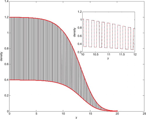
Figure 2. The effect of varying $l_2$ on the accuracy of the leading order approximation of the travelling wave profile. In plots (a–d) $l_2=1.9$ and the numerical non-homogenized solution ρ (black) and leading order approximation ${\rho }_0$ (red) are plotted as a function of the scaled spatial variable ξ (left column) and the unscaled spatial variable x (right column). The first row corresponds to the case where $\alpha =0.25$ andthere is greater preference for patch 2. The second row corresponds to the case where $\alpha =0.75$ and there is greater preference for patch 1. Finally, plot (e) shows the maximum absolute error ($\underset{\xi }{max}|\rho -{\rho }_0|$) as $l_2$ is varied. Plot (f) shows the averaged absolute error across rescaled space ξ. In all cases we ignore population dynamics with $f_1=f_2=0$ and $D_1=D_2=1$ and $l_1=0.1$. We use a Gaussian initial condition and compare solutions at t=3.

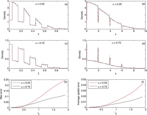
The accuracy of the leading order approximation is affected by patch preference (α) (see (Figure 2 (e,f) and compare (a,b) to (c,d)). We can understand this result by examining the solution profiles. In Figure 2 (a,b), where there is greater preference for patch 2 ($\alpha =0.25$), the population is quick to move through the landscape when compared to Figure 2 (c,d) where preference is for patch 1 ($\alpha =0.75$). The difference in speeds is due to $l_2\gg l_1$. With $l_2\gg l_1$, most of the landscape is of type 2, so when preference is for patch 1 the population movement is slower, the population get ‘stuck’ in small type 1 patches. Once in patch 1 the population has a tendency to stay there and as this patch is small the population cannot travel far. The result of this patch 1 preference is a slower travelling wave and a shallower gradient in population density at the wave front (Figure 2(d)). In contrast, when preference is high for type 2 patches the population moves faster. Although the population now tends to get ‘stuck’ in the large type 2 patches, the larger patch size means the population can still move, generating a faster travelling wave with a steeper gradient in population density at the wave front (Figure 2 (b)). The difference in gradients observed in these travelling wave solutions affects the accuracy of the leading order solution, it is more accurate when the spatial gradient in density is small. The leading order approximation captures the average density on each patch, and so when the spatial variation within a patch is small (small gradient in density, large α) the spatial average is a closer approximation to the within patch density and hence the leading order approximation is more accurate (see Figure 2 (e,f)).

3.1.2. Asymptotic spread rate

The homogenized equation (76(76) ${\mathrm{\partial }}_t\tilde{g}=⟨\tilde{D}{⟩}_h{\mathrm{\partial }}_{\zeta }^2\tilde{g}+(\tilde{\mathrm{\Lambda }}-M\tilde{g})\tilde{g},$(76) ) is the Fisher–KPP equation and so admits travelling wave solutions when $\tilde{\mathrm{\Lambda }}>0$. The asymptotic speed of these travelling wave solutions in ζ-t-coordinates is ${\tilde{c}}^{\ast }=2\sqrt{\tilde{\mathrm{\Lambda }}⟨\tilde{D}{⟩}_h}$, which is given by (78) ${\tilde{c}}^{\ast }=2\left(\frac{2l_1}{l_1+l_2/k}\right)\sqrt{\frac{{\lambda }_1{l}_1+{\lambda }_2{l}_2/k}{l_1/D_1+\left(l_2/k\right)/\left(D_2/k^2\right)}}.$(78) Since a single period has length $2l_1$ in the ξ coordinate, and length $l_1+l_2$ in the y coordinate, the asymptotic speed in x-t-coordinates will be $c^{\ast }={\tilde{c}}^{\ast }(l_1+l_2)/\left(2l_1\right)$, or (79) $c^{\ast }=2\left(\frac{l_1+l_2}{l_1+l_2/k}\right)\sqrt{\frac{{\lambda }_1{l}_1+{\lambda }_2{l}_2/k}{l_1/D_1+\left(l_2/k\right)/\left(D_2/k^2\right)}}.$(79) This result, which matches the asymptotic speed obtained by [12], may be used to approximate the asymptotic speed of periodic travelling wave solutions of the original system (2(2) ${\mathrm{\partial }}_{\tau }\rho =D_i{\mathrm{\partial }}_y^2\rho +{\epsilon }^2{f}_i\left(\rho \right)\mathrm{for}y\in (y_{i-1},y_i),i\in \mathbb{Z}.$(2) ), (3(3) $D_{i+1}{\mathrm{\partial }}_y\rho (y_i^{+},\tau )=D_i{\mathrm{\partial }}_y\rho (y_i^{-},\tau ).$(3) ), (7(7) $\rho (y_i^{+},\tau )=k_i\rho (y_i^{-},\tau ).$(7) ) in x-t-coordinates. In y-τ-coordinates, the asymptotic speed will be smaller by a factor of ϵ as a result of the parabolic scaling.

We compare the asymptotic wave speed prediction with the numerically solved speed obtained from the original non-homogenized system (Equations (2(2) ${\mathrm{\partial }}_{\tau }\rho =D_i{\mathrm{\partial }}_y^2\rho +{\epsilon }^2{f}_i\left(\rho \right)\mathrm{for}y\in (y_{i-1},y_i),i\in \mathbb{Z}.$(2) ), (3(3) $D_{i+1}{\mathrm{\partial }}_y\rho (y_i^{+},\tau )=D_i{\mathrm{\partial }}_y\rho (y_i^{-},\tau ).$(3) ), (7(7) $\rho (y_i^{+},\tau )=k_i\rho (y_i^{-},\tau ).$(7) )) (see Figure 3). In this example we have chosen $l_1=l_2=1$ as well as the intraspecific competition coefficients ${\mu }_i=1$. The asymptotic wave speed prediction has good agreement with the numerically obtained speed. When ${\lambda }_i=1$ the wave speed is maximized when there is no patch preference ($\alpha =0.5$, i.e. k=1). Lowering ${\lambda }_2$, such that growth in patch 2 is lower than in patch 1, we find that wave speed is maximized when $\alpha >0.5$ corresponding to preference for patch 1 over patch 2. This result is expected as the lower ${\lambda }_2$ reduces spread rate in patch 2 and so increased preference for patch 1, where spread rate is higher, can increase the overall wave speed compared to the case of no patch preference ($\alpha =0.5$). However, increasing α too much leads to an eventual decrease in wave speed. A high patch 1 preference reduces entry into patch 2 and hence slowing entry into the next consecutive patch of type 1, ultimately leading to a slower travelling wave solution. As expected, this is in line with findings by [12] who found similar results for the case of linear growth in patch 1 and linear death in patch 2.

Figure 3. Asymptotic wave speed plotted as a function of patch preference, α. The solid line illustrates the homogenized wave speed prediction (Equation 79(79) $c^{\ast }=2\left(\frac{l_1+l_2}{l_1+l_2/k}\right)\sqrt{\frac{{\lambda }_1{l}_1+{\lambda }_2{l}_2/k}{l_1/D_1+\left(l_2/k\right)/\left(D_2/k^2\right)}}.$(79) ) in the case ${\lambda }_1={\lambda }_2=1$, and the dashed line illustrates the case ${\lambda }_1=1$, ${\lambda }_2=0.5$. The grey stars are the numerically simulated wave speeds obtained from solving the original non-homogenized Equations (2(2) ${\mathrm{\partial }}_{\tau }\rho =D_i{\mathrm{\partial }}_y^2\rho +{\epsilon }^2{f}_i\left(\rho \right)\mathrm{for}y\in (y_{i-1},y_i),i\in \mathbb{Z}.$(2) ), (3(3) $D_{i+1}{\mathrm{\partial }}_y\rho (y_i^{+},\tau )=D_i{\mathrm{\partial }}_y\rho (y_i^{-},\tau ).$(3) ), (7(7) $\rho (y_i^{+},\tau )=k_i\rho (y_i^{-},\tau ).$(7) ). The solution was solved until t=50, and the last 30 time steps were used to estimate wave speed, taking a threshold of 0.01 to track the location of the wave front at each time point. In all cases the population dynamics are given by logistic growth ($f_i\left(\rho \right)=({\lambda }_i-{\mu }_i\rho )\rho$), and parameters are $D_1=D_2=1$, ${\mu }_i=1$ and $l_1=l_2=1$.

3.2. Equilibrium densities

In addition to looking at the travelling wave solutions we can also gain ecological insight into the effect of spatial heterogeneity on the equilibrium densities. We can rewrite the reaction term in the homogenized equation (71(71) ${\mathrm{\partial }}_t\tilde{g}=⟨\tilde{D}{⟩}_h{\mathrm{\partial }}_{\zeta }^2\tilde{g}+\left(\frac{l_1}{l_1+l_2/k}\right)\left[f_1\left(\tilde{g}\right)+\left(l_2/l_1\right)f_2\left(\tilde{g}/k\right)\right].$(71) ) (80) ${\mathrm{\partial }}_t\tilde{g}=⟨\tilde{D}{⟩}_h{\mathrm{\partial }}_{\zeta }^2\tilde{g}+\tilde{\mathrm{\Lambda }}(1-\tilde{g}/{\tilde{K}}_{\mathrm{hom}})\tilde{g},$(80) allowing us to compute the carrying capacity for the homogenized model (81) ${\tilde{K}}_{\mathrm{hom}}=\tilde{\mathrm{\Lambda }}/\tilde{M}=\frac{{\lambda }_1{l}_1+{\lambda }_2{l}_2/k}{{\mu }_1{l}_1+{\mu }_2{l}_2/k^2}.$(81) The homogenized equation then admits a non-zero spatially homogeneous equilibrium, $\tilde{g}(\zeta ,t)={\tilde{K}}_{\mathrm{hom}}$, which is positive whenever $\tilde{\mathrm{\Lambda }}$ is positive. At this equilibrium, the leading order solution to the rescaled problem varies periodically, with period $2l_1$ in the ξ-coordinate, or $l_1+l_2$ in the x-coordinate. In x– t-coordinates, the leading order solution ${\rho }_0$ has constant value ${\tilde{K}}_{\mathrm{hom}}$ in each patch of type 1 and constant value ${\tilde{K}}_{\mathrm{hom}}/k$ in each patch of type 2 (see Figure 1). Each patch type (i=1,2) has its own type-specific carrying capacity $K_i={\lambda }_i/{\mu }_i$ if ${\lambda }_i>0$. This is the equilibrium value that would be obtained if the population was spreading through a spatially uniform environment with patch i conditions.

At equilibrium, the leading order solution obtains constant values on patches that generally do not match the patch-specific carrying capacities (${\tilde{K}}_{\mathrm{hom}}\ne K_1$ and ${\tilde{K}}_{\mathrm{hom}}/k\ne K_2$). However, there are some interesting and surprising relationships between these values. We assume without loss of generality that patch 1 has a higher patch-specific intrinsic growth rate than patch 2 (${\lambda }_1>{\lambda }_2$). We also assume that the intrinsic growth rate for the homogenized model is positive ($\tilde{\mathrm{\Lambda }}>0$), so that the spatially uniform equilibrium is positive and stable (${\tilde{K}}_{\mathrm{hom}}>0$). A necessary (but not sufficient) condition for this to occur is ${\lambda }_1>0$.

Under these assumptions, we can use Equation (81(81) ${\tilde{K}}_{\mathrm{hom}}=\tilde{\mathrm{\Lambda }}/\tilde{M}=\frac{{\lambda }_1{l}_1+{\lambda }_2{l}_2/k}{{\mu }_1{l}_1+{\mu }_2{l}_2/k^2}.$(81) ) to derive relationships between the equilibrium densities (${\tilde{K}}_{\mathrm{hom}}$ and ${\tilde{K}}_{\mathrm{hom}}/k$) and the patch-specific carrying capacities ($K_1$ and $K_2$). We consider two cases, ${\lambda }_1>{\lambda }_2>0$ and ${\lambda }_1>0>{\lambda }_2$. In the first case, ${\tilde{K}}_{\mathrm{hom}}$ is always between $K_1$ and $k{K}_2$. This relationship is most interesting when $K_1<k{K}_2$, especially if $K_1>K_2$. When this is true, the presence of patches of type 2 drives the equilibrium density in patches of type 1 above $K_1$, and the presence of patches of type 1 drives the equilibrium density in patch 2 below $K_2$, even though patches of type 1 have a higher patch-specific carrying capacity than patches of type 2. If $K_1>K_2$, then the condition $K_1<k{K}_2$ requires k to be relatively large. Recall that (82) $k=\frac{\alpha }{1-\alpha }\cdot \frac{D_2}{D_1},$(82) where α is the probability that an individual at an interface moves towards the patch of type 1. Thus, k becomes larger as the probability of moving into patch type 1 at an interface increases, or as the motility in patch type 2 (type 1) increases (decreases). The latter increases (decreases) the rate at which individuals in patches of type 2 (type 1) reach the interfaces, and the former determines which patch they enter when they get there. Thus equilibrium densities are strongly influenced by patch-specific carrying capacities as well as the interaction between movement characteristics within the patches and at the interfaces. It is also possible that the equilibrium density in patches of type 2 will be higher than in patches of type 1 in the case that ${\lambda }_1>{\lambda }_2>0$, even if $K_1>K_2$. In fact, this will occur whenever k<1, which reflects a tendency to move into patches of type 2 even though the patch-specific intrinsic growth rate and carrying capacity is lower in those patches.

In the case that ${\lambda }_1>0>{\lambda }_2$, it is still possible to obtain positive equilibrium densities in patches of type 2, even though the intrinsic growth rate is negative in these patches. If ${\lambda }_1>0>{\lambda }_2$, then only patches of type 1 have positive patch-specific carrying capacities, and it is always the case that the equilibrium density in patches of type 1 will be lower than $K_1$.

3.3. Persistence condition

The homogenized model (76(76) ${\mathrm{\partial }}_t\tilde{g}=⟨\tilde{D}{⟩}_h{\mathrm{\partial }}_{\zeta }^2\tilde{g}+(\tilde{\mathrm{\Lambda }}-M\tilde{g})\tilde{g},$(76) ) also suggests a very simple approximate persistence condition, $\tilde{\mathrm{\Lambda }}>0$, or, equivalently (83) ${\lambda }_1{l}_1+{\lambda }_2{l}_2/k>0.$(83) This condition is always satisfied when both patch-specific intrinsic growth rates are positive, and it is never satisfied when both are negative. Thus, we explore the more interesting case when ${\lambda }_1>0>{\lambda }_2$. First, we note that although the approximate persistence condition (83(83) ${\lambda }_1{l}_1+{\lambda }_2{l}_2/k>0.$(83) ) is derived easily from the homogenized model (76(76) ${\mathrm{\partial }}_t\tilde{g}=⟨\tilde{D}{⟩}_h{\mathrm{\partial }}_{\zeta }^2\tilde{g}+(\tilde{\mathrm{\Lambda }}-M\tilde{g})\tilde{g},$(76) ), it may also be derived as an approximation to the exact persistence boundary obtained by [12]. Using our notation, their exact persistence boundary reads (84) $k\tan \left(\frac{l_1}{2}\sqrt{\frac{{\lambda }_1}{D_1}}\right)=\sqrt{\frac{-{\lambda }_2{D}_2}{{\lambda }_1{D}_1}}\tanh \left(\frac{l_2}{2}\sqrt{\frac{-{\lambda }_2}{D_2}}\right).$(84) Since, $l_1$ and $l_2$ are small ($O\left(\epsilon \right)$), we approximate the tangent and hyperbolic tangent using Maclaurin series ($\tan \left(x\right)=x+O\left(x^3\right)$ and $\tanh \left(x\right)=x+O\left(x^3\right)$), yielding (85) $k\left(\frac{l_1}{2}\sqrt{\frac{{\lambda }_1}{D_1}}\right)\approx \sqrt{\frac{-{\lambda }_2{D}_2}{{\lambda }_1{D}_1}}\left(\frac{l_2}{2}\sqrt{\frac{-{\lambda }_2}{D_2}}\right).$(85) Simplifying, we obtain (86) $l_1{\lambda }_1\approx -{\lambda }_2{l}_2/k,$(86) which is the same persistence boundary as (83(83) ${\lambda }_1{l}_1+{\lambda }_2{l}_2/k>0.$(83) ).

Though the persistence condition (83(83) ${\lambda }_1{l}_1+{\lambda }_2{l}_2/k>0.$(83) ) is approximate, it is valid for small patch widths, and it is much simpler than the exact condition (84(84) $k\tan \left(\frac{l_1}{2}\sqrt{\frac{{\lambda }_1}{D_1}}\right)=\sqrt{\frac{-{\lambda }_2{D}_2}{{\lambda }_1{D}_1}}\tanh \left(\frac{l_2}{2}\sqrt{\frac{-{\lambda }_2}{D_2}}\right).$(84) ). It also readily yields important theoretical insights. The approximate persistence condition suggests that invasion will occur whenever a weighted average of the patch-specific intrinsic growth rates is positive. The corresponding weights, $l_1$ and $l_2/k$ have an appealingly simple biological interpretation. In the original model (2(2) ${\mathrm{\partial }}_{\tau }\rho =D_i{\mathrm{\partial }}_y^2\rho +{\epsilon }^2{f}_i\left(\rho \right)\mathrm{for}y\in (y_{i-1},y_i),i\in \mathbb{Z}.$(2) ), (3(3) $D_{i+1}{\mathrm{\partial }}_y\rho (y_i^{+},\tau )=D_i{\mathrm{\partial }}_y\rho (y_i^{-},\tau ).$(3) ), (7(7) $\rho (y_i^{+},\tau )=k_i\rho (y_i^{-},\tau ).$(7) ), 1 and 1/k give the residence indices within patches of types 1 and 2, respectively. The residence index is proportional to the equilibrium population density and inversely proportional to motility [24]. Scaling the residence indices by the corresponding patch extent ($l_i$ in the x direction, and unit extent in the perpendicular direction) gives the residence times [18] for the two patch types, which are equal to the weights $l_1$ and $l_2/k$. The residence time for a patch type is proportional to the amount of time that individuals will spend in that patch type at equilibrium. Thus, we may interpret the persistence condition (83(83) ${\lambda }_1{l}_1+{\lambda }_2{l}_2/k>0.$(83) ) to say that the intrinsic rate of growth in patches of type 1 multiplied by the relative amount of time spent in those patches at equilibrium must exceed the intrinsic rate of decline within patches of type 2 multiplied by the relative amount of time spent in those patches at equilibrium.

4. Discussion

The dynamics of populations on large spatial and temporal scales are of great interest in theoretical ecology, for example in conservation and invasion biology. Empirical work, however, typically considers individual behaviour on small spatial and temporal scales. Understanding how processes on a small scale impact patterns on larger scales is a fundamental challenge in ecology. Reaction–diffusion equations are a natural framework to study such questions since they allow the inclusion of individual-level movement rules into equations for population densities [4]. These equations have provided many important insights into processes in spatial ecology, but typically assume that population densities are continuous. Recent work on modelling individual movement behaviour at sharp habitat edges expanded the framework of reaction–diffusion equations to include aspects such as habitat preference, for which many empirical studies exist, see [12] and references therein. It turns out that not only the coefficient functions but also the population density is discontinuous at interfaces [12,16]. Our work here contributes to the understanding of this relatively novel aspect of reaction–diffusion equations.

Homogenization methods have a long and distinguished history in the qualitative analysis of reaction–diffusion equations [2,9,17]. If the coefficient functions in a reaction–diffusion equation vary on a small spatial scale, then an appropriate average over that small scale yields a reaction–diffusion equation with constant coefficients on a larger scale as a zero-order approximation. While this asymptotic result holds in the limit as the small scale goes to zero, the resulting large-scale equation provides a surprisingly good approximation far from the small-scale limit. However, the known homogenization methods either assume continuous density functions [15], are restricted to the special case of no habitat preference at patch interfaces [7], or rely on spatial rescaling to make the population density continuous [13]. The main result of our work is the development of corresponding techniques for general interface conditions that do not depend on rescaling. As a result, the techniques developed here are applicable to a broader range of models, including multispecies systems. It turns out that while the limiting equations have a simple form that is similar to the case of continuous densities [15], the arguments, and calculations that lead to them are quite a bit more involved than in that case.

While a number of qualitative results are available, a rigorous analytical investigation of the type of reaction–diffusion equations with discontinuity conditions at interfaces is still in its infancy. But the discontinuities of the density is not only an analytical challenge. Numerical schemes to resolve the discontinuities need to be developed along with corresponding convergence and error estimates. We used a second-order finite difference scheme to match densities and fluxes across an interface and applied a spatially implicit, temporally explicit fractional step method known as Strang-splitting [26]. We found an excellent agreement of the homogenized solution to the numerical solution of the exact equations.

The simple form of the homogenized equation enables us to obtain analytical results that cannot be easily obtained from the non-homogenized equation directly. As an example of this, the persistence condition for the logistic example demonstrates that patch residence time plays a key role in determining population persistence and we are able to directly relate patch residence time to the small-scale characteristics of individual movement at and near the patch interfaces. In particular, if at a patch interface the probability of moving into patch 1 is high then the patch 2 residence time will be low unless motility in patch 2 is much lower than patch 1 or the size of patch 2 is much larger than patch 1. Hence, we can see how the small-scale processes trade off against one another to give landscape-scale behaviour.

Probably the most surprising ecological result from our numerical examples is that the carrying capacity of the homogenized equation can be higher than the highest carrying capacity in the small-scale equation. While the equilibrium population density in the homogenized model cannot exceed the homogenized carrying capacity, the density on the small-scale model can and does, as we see in the numerical simulations (see Figure 1). The mechanism behind this ‘overshooting’ of the carrying capacity is the preference of individuals for these patches. The carrying capacities in the two patch types are $K_i={\lambda }_i/{\mu }_i.$ In dimensional terms, the carrying capacity of the homogenized model is given by (87) $K_{\mathrm{hom}}=\tilde{\mathrm{\Lambda }}/\tilde{M}=\left(\frac{{\lambda }_1{l}_1+{\lambda }_2{l}_2/k}{l_1+l_2/k}\right){\left(\frac{\left({\mu }_1\right)l_1+\left({\mu }_2/k\right)l_2/k}{l_1+l_2/k}\right)}^{-1}.$(87) The numerator of this expression is a weighted average of the growth rates with weights $l_1$ and $l_2/k$, and as we saw in Section 3.3, these weights are, respectively, the patch 1 and 2 residence times. The denominator of $K_{\mathrm{hom}}$ is an average of the modified intraspecific competition coefficients ${\mu }_1$ and ${\mu }_2/k$ also with the same weights. In Section 3.3 we noted that 1 and 1/k in these modified competition coefficients are proportional to the equilibrium patch 1 and 2 densities. Thus, we can regard ${\mu }_1$ and ${\mu }_2/k$ as scaled competition coefficients, scaled by patch density. The factor $k=\left(\alpha D_2\right)/\left(\right(1-\alpha \left)D_1\right)$ that appears in the various weights incorporates the movement rates in the patches adjacent to the interface as well as movement preference (see Equation (82(82) $k=\frac{\alpha }{1-\alpha }\cdot \frac{D_2}{D_1},$(82) )). In other words, the small-scale characteristics of individual movement at and near an interface enters the population growth function on the large scale through the homogenization procedure. A similar phenomenon was implicitly observed but not discussed in a model with Allee effect, where the homogenization required a prior scaling to obtain continuous population densities [13]. The method presented here is much more general. In particular, it is applicable to models of two or more interacting populations. It will be particularly interesting and ecologically important to study how the small-scale movement characteristics of the various populations enter and modify the population growth functions on the large scale. This question is the subject of future work.

Acknowledgements

We thank Frithjof Lutscher for many helpful discussions during this work and during the preparation of this manuscript. We also thank two anonymous reviewers for their useful comments on this manuscript.

Disclosure statement

The authors declare that they have no conflicts of interest.

ORCID

Brian P. Yurk http://orcid.org/0000-0003-1134-8566

Additional information

Funding

This work was supported by the American Institute of Mathematics SQuaREs Program. Brian P. Yurk was supported by a Jacob E. Nyenhuis Faculty Development Grant from Hope College.

Appendix. Numerical simulation

A.1. Numerical algorithm

To solve the non-homogenized reaction–diffusion problem (Equations (2(2) ${\mathrm{\partial }}_{\tau }\rho =D_i{\mathrm{\partial }}_y^2\rho +{\epsilon }^2{f}_i\left(\rho \right)\mathrm{for}y\in (y_{i-1},y_i),i\in \mathbb{Z}.$(2) ), (3(3) $D_{i+1}{\mathrm{\partial }}_y\rho (y_i^{+},\tau )=D_i{\mathrm{\partial }}_y\rho (y_i^{-},\tau ).$(3) ), (7(7) $\rho (y_i^{+},\tau )=k_i\rho (y_i^{-},\tau ).$(7) )) we use a fractional step method, which involves treating the PDE as a sequence of disjoint operations. If we let $\mathcal{D}$ denote the diffusion operator and $\mathcal{R}$ denote the reaction operator, then we can obtain a numerical scheme that is second order accurate in time and space using the fractional step method Strang-splitting [25,26]. Let $u^n$ be the solution of the PDE at time $t_n$ then we can obtain $u^{n+1}$, a numerical approximation of the solution at time $t_{n+1}=t_n+\mathrm{\Delta }t$, as follows: $u^{n+1}=\mathcal{D}\left(\mathrm{\Delta }t/2\right)\mathcal{R}\left(\mathrm{\Delta }t\right)\mathcal{D}\left(\mathrm{\Delta }t/2\right)u^n.$ Thus we apply half a time step of diffusion ($\mathcal{D}\left(\mathrm{\Delta }t/2\right)$) followed by a full time step of reaction ($\mathcal{R}\left(\mathrm{\Delta }t\right)$) and then another half a time step of diffusion.

As the diffusion and reaction steps in this method are now independent we can choose second-order accurate numerical schemes for approximating $\mathcal{D}$ and $\mathcal{R}$. For the diffusion step we use Crank–Nicolson, and for the reaction step we use fourth order Runge–Kutta. When applying the Crank–Nicolson step we have the additional complication of the interface conditions at each patch boundary. To ensure the whole scheme remains second-order accurate we use second-order forward or backward difference to approximate the derivatives in the interface conditions (Equations (3(3) $D_{i+1}{\mathrm{\partial }}_y\rho (y_i^{+},\tau )=D_i{\mathrm{\partial }}_y\rho (y_i^{-},\tau ).$(3) ), (7(7) $\rho (y_i^{+},\tau )=k_i\rho (y_i^{-},\tau ).$(7) )). As density may be discontinuous across the interface, we need to introduce two nodes at an interface location. One of these nodes (j) corresponds to the interface on the right-hand side of the patch to the left of the interface, and the other node (j+1) corresponds to the interface on the left-hand side of the patch to the right of the interface. Thus if we consider an interface with a patch of type 1 (type 2) located to the right (left) then at each time step n the interface conditions (3(3) $D_{i+1}{\mathrm{\partial }}_y\rho (y_i^{+},\tau )=D_i{\mathrm{\partial }}_y\rho (y_i^{-},\tau ).$(3) ), and (7(7) $\rho (y_i^{+},\tau )=k_i\rho (y_i^{-},\tau ).$(7) ) are expressed as (88) $\begin{array}{rl}& u_{j+1}^n=k{u}_j^n,\end{array}$(88) (89) $\begin{array}{rl}& D_1\frac{(-3u_{j+1}^n+4u_{j+2}^n-u_{j+3}^n)}{2\mathrm{\Delta }x}=D_2\frac{(3u_j^n+4u_{j-1}^n+u_{j-2}^n)}{2\mathrm{\Delta }x},\end{array}$(89) where $u_j^n$ is the value of the solution at time $t_n$ at grid point j and $\mathrm{\Delta }x$ is the spatial step. In the numerical simulations presented in the paper we chose $\mathrm{\Delta }t=1\times {10}^{-4}$ and $\mathrm{\Delta }x=1\times {10}^{-3}$.

A.2. Initial conditions

In order to compare the travelling wave profile $\rho (x,y,t)$ of the original non-homogenized equations (2(2) ${\mathrm{\partial }}_{\tau }\rho =D_i{\mathrm{\partial }}_y^2\rho +{\epsilon }^2{f}_i\left(\rho \right)\mathrm{for}y\in (y_{i-1},y_i),i\in \mathbb{Z}.$(2) ), (3(3) $D_{i+1}{\mathrm{\partial }}_y\rho (y_i^{+},\tau )=D_i{\mathrm{\partial }}_y\rho (y_i^{-},\tau ).$(3) ), (7(7) $\rho (y_i^{+},\tau )=k_i\rho (y_i^{-},\tau ).$(7) ) to the leading order approximation ${\rho }_0(x,y,t)=g(x,t)/h\left(y\right)$ care needs to be taken to choose appropriate initial conditions for $\rho (x,y,t)$. Taking a Gaussian for the initial condition for $g(x,0)$ in the homogenized equation (69(69) ${\mathrm{\partial }}_{t}g=⟨D{⟩}_h{\mathrm{\partial }}_x^{2}g+\left(\frac{1}{1+1/k}\right)\left[f_1\left(g\right)+f_2\left(g/k\right)\right],$(69) ), then we take $\rho (x,y,0)=g(x,t)/h\left(y\right)$ as the initial condition for the original PDE (2(2) ${\mathrm{\partial }}_{\tau }\rho =D_i{\mathrm{\partial }}_y^2\rho +{\epsilon }^2{f}_i\left(\rho \right)\mathrm{for}y\in (y_{i-1},y_i),i\in \mathbb{Z}.$(2) ).

References

- J. Belmonte-Beitia, T.E. Woolley, J.G. Scott, P.K. Maini, and E.A. Gaffney, Modelling biological invasions: Individual to population scales at interfaces, J. Theor. Biol. 334 (2013), pp. 1–12. doi: 10.1016/j.jtbi.2013.05.033
- A. Bensoussan, J. Lions, and G. Papanicolaou, Asymptotic Analysis for Periodic Structures, North-Holland, Amsterdam, 1978.
- R.S. Cantrell and C. Cosner, Diffusion models for population dynamics incorporating individual behavior at boundaries: Applications to refuge design, Theor. Popul. Biol. 55 (1999), pp. 189–207. doi: 10.1006/tpbi.1998.1397
- R.S. Cantrell and C. Cosner, Spatial Ecology via Reaction–Diffusion Equations, Mathematical and Computational Biology, Wiley, New York, 2003.
- G. Cruywagen, P. Kareiva, M. Lewis, and J. Murray, Competition in a spatially heterogeneous environment: Modelling risk of spread of a genetically engineered population, J. Math. Biol. 49 (1996), pp. 1–38.
- S. Dewhirst and F. Lutscher, Dispersal in heterogeneous habitats: Thresholds, spatial scales, and approximate rates of spread, Ecology 90 (2009), pp. 1338–1345. doi: 10.1890/08-0115.1
- M.J. Garlick, J.A. Powell, M.B. Hooten, and L.R. MacFarlane, Homogenization of large-scale movement models in ecology, Bull. Math. Biol. 73 (2011), pp. 2088–2108. doi: 10.1007/s11538-010-9612-6
- K.J. Haynes and J.T. Cronin, Interpatch movement and edge effects: The role of behavioral responses to the landscape matrix, Oikos 113 (2006), pp. 43–54. doi: 10.1111/j.0030-1299.2006.13977.x
- M.H. Holmes, Introduction to Perturbation Methods, Springer, New York, 2013.
- N. Kinezaki, K. Kawasaki, F. Takasu, and N. Shigesada, Modeling biological invasions into periodically fragmented environments, Theor. Popul. Biol. 64 (2003), pp. 291–302. doi: 10.1016/S0040-5809(03)00091-1
- F. Lutscher, Non-local dispersal and averaging in heterogenous landscapes, Appl. Anal. 87 (2010), pp. 1091–1108. doi: 10.1080/00036811003735816
- G.A. Maciel and F. Lutscher, How individual movement response to habitat edges affects population persistence and spatial spread, Am. Nat. 182 (2013), pp. 42–52. doi: 10.1086/670661
- G.A. Maciel and F. Lutscher, Allee effects and population spread in patchy landscapes, J. Biol. Dyn. 9 (2015), pp. 109–123. doi: 10.1080/17513758.2015.1027309
- R.C. Neupane and J.A. Powell, Invasion speeds with active dispersers in highly variable landscapes: Multiple scales, homogenization, and the migration of trees, J. Theor. Biol. 387 (2015), pp. 111–119. doi: 10.1016/j.jtbi.2015.09.029
- H.G. Othmer, A continuum model for coupled cells, J. Math. Biol. 17 (1983), pp. 351–369. doi: 10.1007/BF00276521
- O. Ovaskainen and S.J. Cornell, Biased movement at a boundary and conditional occupancy times for diffusion processes, J. Appl. Prob. 40 (2003), pp. 557–580. doi: 10.1017/S0021900200019562
- G.A. Pavliotis and A.M. Stuart, Multiscale Methods: Averaging and Homogenization, Springer, New York, 2008.
- J.A. Powell and N.E. Zimmermann, Multiscale analysis of active seed dispersal contributes to resolving Reid's paradox, Ecology 85 (2004), pp. 490–506. doi: 10.1890/02-0535
- O.J. Robertson and J.Q. Radford, Gap-crossing decisions of forest birds in a fragmented landscape, Aust. Ecol. 34 (2009), pp. 435–446.
- N. Schtickzelle and M. Baguette, Behavioural responses to habitat patch boundaries restrict dispersal and generate emigration-patch area relationships in fragmented landscapes, J. Anim. Ecol. 72 (2003), pp. 533–545. doi: 10.1046/j.1365-2656.2003.00723.x
- C.B. Schultz and E.E. Crone, Edge-mediated dispersal behavior in a prairie butterfly, Ecology 82 (2001), pp. 1879–1892. doi: 10.1890/0012-9658(2001)082[1879:EMDBIA]2.0.CO;2
- N. Shigesada, K. Kawasaki, and E. Teramoto, Traveling periodic waves in heterogeneous environments, Theor. Popul. Biol. 30 (1986), pp. 143–160. doi: 10.1016/0040-5809(86)90029-8
- N. Shigesada, K. Kawasaki, and H.F. Weinberger, Spreading speeds of invasive species in a periodic patchy environment: Effects of dispersal based on local information and gradient-based taxis, Japan J. Indust. Appl. Math. 32 (2015), pp. 675–705. doi: 10.1007/s13160-015-0191-7
- P. Turchin, Quantitative Analysis of Movement: Measuring and Modeling Population Redistribution in Animals and Plants, Sinauer, Sunderland, MA, 1998.
- R. Tyson, Pattern Formation by E. Coli and S. Typhimurium – Mathematical and numerical investigation of a biological phenomenon, Ph.D. diss., University of Washington, 1996.
- R. Tyson, L.G. Stern, and R.J. LeVeque, Fractional step methods applied to a chemotaxis model, J. Math. Biol. 41 (2000), pp. 455–475. doi: 10.1007/s002850000038
- H.F. Weinberger, M.A. Lewis, and B. Li, Analysis of linear determinacy for spread in cooperative models, J. Math. Biol. 45 (2002), pp. 183–218. doi: 10.1007/s002850200145