?Mathematical formulae have been encoded as MathML and are displayed in this HTML version using MathJax in order to improve their display. Uncheck the box to turn MathJax off. This feature requires Javascript. Click on a formula to zoom.
ABSTRACT
Explicit expressions in terms of Gaussian Hypergeometric functions are found for a ‘balance’ manifold that connects the non-zero steady states of a 2-species, non-competitive, scaled Lotka–Volterra system by the unique heteroclinic orbits. In this model, the parameters are the interspecific interaction coefficients which affects the form of the solution used. Similar to the carrying simplex of the competitive model, this balance simplex is the common boundary of the basin of repulsion of the origin and infinity, and is smooth except possibly at steady states.
1. Background
For a Lotka–Volterra system with 2-species, the phase portraits are well known [Citation7,Citation16,Citation19]. However, explicit solutions are rare, whether for actual solutions [Citation20,Citation28], or for invariant manifolds [Citation6,Citation31]. Here we obtain an explicit and analytic solution for the heteroclinic orbits that connect non-zero steady states in a scaled Lotka–Volterra system (see (Equation1(1)
(1) ) below). This solution, which we call a balance simplex Σ, attracts all non-zero solutions and is invariant under the flow of the system. It also divides the phase plane into two distinct regions. The lower region (containing the origin) has solutions which are repelled by the origin. The unbounded region above Σ has solutions in the phase plane which are declining from infinity.
In the case where both species compete against one another, for our model Σ is precisely the carrying simplex introduced by Hirsch [Citation14]. The carrying simplex is a Lipschitz manifold that attracts all non-trivial solutions and has been studied in more general and higher dimensional systems (for continuous time see, for example, [Citation2,Citation14,Citation26] and for discrete-time [Citation17,Citation18]). Our solution Σ provides an explicit example of an analogue of the carrying simplex which also applies to predator-prey type or a co-operative interactions. Figure shows schematic views of the carrying simplex and the balance simplex.
Figure 1. A general diagram of a carrying simplex (left) and balance simplex (right) in red. The diagonal blue line is the unit simplex and the orange points are steady states of the system. The grey curves are solution trajectories of the system.
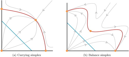
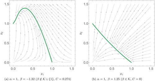
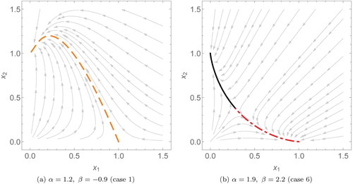
Figure 2. Phase plots of two species scaled Lotka–Volterra systems in the -plane. These four plots cover the generic qualitative dynamics of the system with different interspecific interaction coefficients (α and β). The orange points are the steady states of the system and the arrows show how solution trajectories evolve over time.
Note (a) does not apply to the strongly co-operative case (
and
) where all positive solutions are unbounded.
2. Introduction
Consider what we call the 2-species scaled Lotka–Volterra system, where all intrinsic growth rates are equal to 1 and the intraspecific interaction coefficients for both species are 1. The former condition means that the origin is always an unstable node, and the latter condition ensures there are no periodic orbits in [Citation16]. Taken together these conditions also mean that each species has a normalised carrying capacity of 1, i.e. we have two axial steady states:
and
. The resulting system is:
(1)
(1) We make the following
Standing assumption: The interspecific interaction coefficients α and β can be of any sign or zero, but .
(The case where one of is equal to 1 is covered in the appendix.) Note that all solutions are repelled from infinity apart from in the strongly co-operative case (where both
and
) which we do not consider as all positive solutions will be unbounded, in which case the concept of the balance simplex is not applicable.
Whilst (Equation1(1)
(1) ) may seem like quite a restricted system (since we have set four of our original parameters to the value 1), any general 2-species system with equal, non-zero intrinsic growth rates
and non-zero intraspecific interaction coefficients
can be written as a scaled Lotka-Volterra system with the change of variables
. This follows from the remark before equation
in Tineo [Citation26] (after correcting the expression in their argument of
).
The system (Equation1(1)
(1) ) has at most one interior steady state,
, which we say exists when
, i.e. when both
or both
and
.
Definition 2.1
For the system (Equation1(1)
(1) ), we define the balance simplex Σ to be a manifold with the following properties:
Σ is invariant, compact and projects radially 1-1 and onto the unit probability simplex;
Σ globally attracts all non-zero points in
.
Thus Σ is compact, connected and contains all non-zero steady states, and Σ separates solutions which are repelled by the origin from those which decline from infinity. Σ is the boundary of the basin of repulsion of the origin and of infinity. In this paper, we focus on constructing Σ explicitly, as an analytic solution to the system (Equation1(1)
(1) ).
Although it is possible to argue that Σ exists for our model (Equation1(1)
(1) ) using topological arguments, it is convenient to use Bomze's classification of the phase portrait for planar Lotka–Volterra systems [Citation7,Citation8]. Using Bomze's link between Lotka-Volterra and 3-species replicator dynamics on the
dimensional simplex, we conclude that (Equation1
(1)
(1) ) when transformed to a replicator system should have a repelling simplex vertex connected to two simplex edges, each of which contains an interior steady state (the third edge corresponds to points at infinity). The only such portraits in [Citation7] are labelled 1, 5, 7, 8, 9, 10, 34, 35, 37, 38. Inspection shows that all these portraits have a manifold that connects the two edge steady states, and that attracts all points except the repelling vertex and points on the edge opposite to the repelling vertex, so we may establish by way of Bomze's classification:
Lemma 2.2
When the planar system (Equation1
(1)
(1) ) has a compact and connected 1-dimensional invariant manifold Σ that globally attracts all non-zero solutions, and contains all non-zero steady states and the heteroclinic orbits connecting them (Figure ).
3. Explicit expressions for the balance simplex
In this section we explicitly construct the balance simplex of Lemma 2.2 for all .
We begin by transforming (Equation1(1)
(1) ) into polar co-ordinates:
With some simplification, we can write:
where
and
.
To work with rational functions, we use the substitution . Note that we are only interested in the first quadrant,
(i.e.
) and
. Using the chain rule, we can now write
(2)
(2) The differential Equation (Equation2
(2)
(2) ) can be solved using the following integrating factor:
(3)
(3) where
and
, i.e.
. Multiplying by this integrating factor, then integrating we obtain formally
(4)
(4) where C is a constant. If
is a local solution of (Equation2
(2)
(2) ) passing through the point
where
, then
is a local solution of (Equation1
(1)
(1) ) passing through the point
where
and
. Different choices of
determine the constant C in (Equation4
(4)
(4) ).
We define
(5)
(5) where
(which may be positive or negative – recall that we restrict
). Depending on
, and the value of T, the integral
may not always converge, and this determines the range of values of T for which the local solution to (Equation2
(2)
(2) ) can be extended. Formally, our solution would then be:
(6)
(6) for which the balance manifold is given parametrically in
co-ordinates by
, where
is the interval where (Equation6
(6)
(6) ) converges.
To provide an alternative solution form when the solution above fails to converge, it is useful to note a symmetry in this problem. If are swapped, this is equivalent to swapping the index of the two species without changing the dynamics. In the phase plane, this is equivalent to a reflection on
, i.e. the axes are swapped. We can return to our original dynamics by re-indexing the two species, which we can do in the form of the transformation
. With this in mind, we define
(7)
(7)
(8)
(8) where
. Using (Equation7
(7)
(7) ) and (Equation8
(8)
(8) ) we obtain a second solution to (Equation2
(2)
(2) ):
(9)
(9) where
is a constant of integration. For clarity, we will add the subscript ‘1’ to our first solution (and
):
(10)
(10) We will explore solutions to (Equation2
(2)
(2) ) made from
and
for different parameters α and β in order to find an explicit expression for the balance simplex.
Remark 1
We note that solutions with appropriate constants
or
can be used to describe all orbits of (Equation1
(1)
(1) ), but this is not the focus of our study. Rather we are concerned with the balance simplex which is constructed from special orbits of (Equation2
(2)
(2) ), namely heteroclinic orbits.
The forthcoming analysis derives valid ranges we can use the solutions in different parameter cases (see Figure ) and a summary is given in Table .
Figure 3. The parameter space with the different cases shown, each extending to infinity. Note that in the region of unbounded dynamics (both
and
), the balance simplex does not exist.
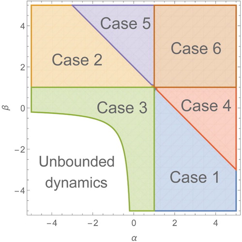
Table 1. The valid ranges in T for which we can use the solutions and in different parameter cases α and β. The remaining case (case 6) where both uses a slightly different solution and will be discussed later. A region plot of these cases can be found in Figure .
4. Construction of the heteroclinic orbits
Now we will determine which constants and
correspond to the solution connecting all the non-zero steady states by explicitly examining the limits of the solutions
and
. We will make use of two important results on the convergence of integrals (p-integral test):
In what follows we use that when the interior steady state
exists, its position with respect to the variable T is given by
. For
,
exists if and only if
. We write
.
4.1. Case 1: and .
Here ,
and
, so that there is no interior steady state. In this case we expect the balance simplex to consist of a single heteroclinic orbit connecting
and
. We use the first solution
since
for
. Next we determine the constant C in (Equation6
(6)
(6) ) so that the balance simplex passes through
at T=0 and
at
.
(a)
For the limit of as
, we have a potential problem with the
in the denominator of the term with the constant
in equation (Equation6
(6)
(6) ). However, if we set
, then we can calculate the limit
which in our original co-ordinates means
, the axial steady state on the
axis.
(b)
The leading order of as
is
, thus
is unbounded
. Note that
, so from I2 and equation (Equation5
(5)
(5) ),
is also unbounded as
. We consider the limit of
using L'Hôpital's rule:
where
With some simplifications, we can show:
It is worth noting that the limit has this value regardless of the constant of integration
. This is expected as the axial state
is locally attracting with these parameters.
We can conclude that with the choice of , the solution
corresponds to the balance simplex in
co-ordinates, joining both axial steady states.
4.2. Case 2: and
For our domain ,
which will be complex when raised to the power ξ, however
here so we consider the second solution,
, instead. This parameter space is equivalent to the case where
and
; this is Case 1 with α and β exchanged. The solution is thus obtained analogously from Case 1 by exchanging α and β, and the variable T with
everywhere in the calculations since we are now using the second solution. The balance simplex Σ is thus given by
with
which joins the two axial steady states.
4.3. Case 3: and .
The inequality is required for boundedness of all solutions; without it, the balance simplex does not always exist. Here
,
and
, so that there is an interior steady state. To construct the balance simplex will need to join together the two solutions
and
at the interior steady state
.
(a)
Near T=0, and we can calculate the limit of
as done previously, making the choice of
for boundedness:
.
(b) , i.e.
For large T, we consider the solution since
when
. We can use the analogous calculations in case 3a if we consider
small. With the choice of
:
.
(c)
We first consider this limit from below, , where only the first solution
is real. Since
,
behaves like I1; we know that
is unbounded as
. The function
is also unbounded as
, again using
. This means we can examine this limit of
using L'Hôpital's rule. We have:
(11)
(11) which matches the value
obtained from polar co-ordinates at the interior steady state
. This is a valid conclusion for any constant of integration
, consistent with
being attracting. We could also do an analogous calculation for the limit
. Here the second solution
is real and we would consider the limit
which gives exactly the same limit value as
.
We conclude that by choosing , we have a solution which connects each axial steady state to the interior steady state, thus giving the balance simplex.
4.4. Case 4: and .
Here ,
and
, so that there is no interior steady state. We use the first solution
.
(a)
Once again, if we set , then we find
, corresponding to
.
(b)
It is clear from I2 and equation (Equation5(5)
(5) ) that
is unbounded as
since the leading order of its integrand is
. The leading order of
is
and so
is also unbounded as
and we can again apply L'Hôpital's rule on
to conclude
for any constant
, consistent with
being attracting.
Hence with , the solution
corresponds to the balance simplex joining both axial steady states.
4.5. Case 5: and .
Here, we use the second solution, , since
. Equivalently, this case is where
and
which has been covered analogously in Case 4 with the first solution
. The balance simplex Σ is thus given by
with
.
4.6. Case 6: .
Here ,
and
, so that there is an interior steady state. As in Case 4 we will join
and
at
.
(a)
In this case if and only if
. Thus for large T we now consider the modification:
(12)
(12) where
(13)
(13) The integrand has leading order
since
. This means
is unbounded as
using I2. The leading order of
is
and so
is also unbounded as
and we can apply L'Hôpital's rule,
(14)
(14) This follows exactly the same calculation as in case 1b, thus we can conclude
, regardless of the constant of integration
, consistent with
being attracting.
(b) , i.e.
For small T (i.e. large ), since
when
we consider the modification:
(15)
(15) where
(16)
(16) Using the analogous calculations from case 6a,
is unbounded as
, and the same is true for
. Thus we can apply L'Hôpital's rule to conclude that
converges to 1 as
, i.e. as
, regardless of the constant
, consistent with
being attracting.
(c)
Another point we must examine is since
and
. We first examine the limit from above (
) where
remains real. It is clear that
and
.
Since , if
, then
is unbounded as
. Setting
, we can use L'Hôpital's rule to examine the limit of
as
. This follows the calculation from case 3c, but we must be careful with the sign of
when simplifying and bringing terms into the square root:
(17)
(17) which matches the value of
at the interior steady state
. Since we expect
to lie on the balance simplex,
is indeed the correct constant for the balance simplex.
We can also do an analogous calculation for the limit of as
(i.e. as
), which gives exactly the same limit value with the choice of
.
Thus, for the case where both we use the modified solution
with
in the range
and
with
in
for the balance simplex.
5. Σ is a balance simplex
Recall that the general solution R to (Equation2(2)
(2) ) was found by transforming the scaled Lotka–Volterra system into polar co-ordinates, then using the substitution
. The constants
and/or
were set to 0 to find the balance simplex. This gives a simple parametric form of our solution, for example, for
:
(18)
(18) Let
,
, be our complete solution to (Equation2
(2)
(2) ), equal to
or
in the appropriate ranges of T, with the constants of integration
and/or
set to 0. We have seen that parametrically
and the function
is injective. We can therefore map our solution to the unit simplex using
where
is the relative frequency of species 1. Thus our two dimensional balance simplex is homeomorphic to the unit 1-simplex by radial projection.
Lemma 2.2 confirms that the invariant manifold Σ attracts all points except the origin and hence Σ is a balance simplex.
6. Simplifications that use the Gaussian hypergeometric function
The Gaussian hypergeometric function (GHF) [Citation4,Citation5,Citation29] is defined for by
(19)
(19) where the Pochhammer symbol means
and
for a positive integer k. This power series in z is defined when c is not equal to a non-positive integer and converges if
.
The GHF also has the following integral representation which converges if and
[Citation4]:
(20)
(20) where Γ is the Gamma function:
(21)
(21) which converges absolutely when
. We now show that we can actually write our solutions
,
,
and
in terms of GHFs.
We will also make use of Euler's transformation of the hypergeometric function [Citation4, pp. 64], derived from the substitution in the integral representation (Equation20
(20)
(20) ):
(22)
(22) We can now write the integral
(Equation5
(5)
(5) ) for
in the following way, using
,
,
, and also that
,
(23)
(23) giving the general solution for
:
(24)
(24) Similarly, recalling that we use
to denote
,
(25)
(25) giving the general solution for
:
(26)
(26) Remark: The third argument of
in
(respectively
) is a non-positive integer when β (respectively α) belongs to the set:
(27)
(27) note that
. From Table we can see that we only use
in the case where
, thus
and the GHF in equation (Equation24
(24)
(24) ) is well defined. Similarly,
is only used in cases where
.
The integrals (Equation13
(13)
(13) ) and
(Equation16
(16)
(16) ) (from case 6 where both
) can also be written in terms of GHFs:
Applying Euler's transformation, we have
Hence the general solution for
when
is
Similarly,
and so after applying the Euler transformation, the general solution for
is
Remark 2
For both and
the third argument of their GHFs is a non-positive integer k when
(28)
(28) Note that the numerator and denominator are both positive since
and k is a non-positive integer. Using
we can also see that
implying
in (Equation28
(28)
(28) ). Thus when using
and
, their GHFs are always defined since we only use them in the case where both
.
7. Summary of explicit solutions
Recall that and note that
. When we write
, it means the Gaussian hypergeometric function defined as the series in the previous section, along with its analytic continuaton.
8. Example plots for different species-species interactions
Some phase plots with example parameters for α and β showing the balance simplex can be found in Figures and .
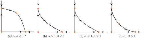
Figure 4. Phase plots of two species scaled Lotka–Volterra systems with different interspecific interaction coefficients (α and β). Here (a) and (b) are competitive systems, (c) is a co-operative system and (d) is an example of predation. In these plots, the solutions (dashed, orange) and
(solid, green) only meet at the interior steady state
.

Figure 5. Phase plots of two species scaled Lotka–Volterra systems with different interspecific interaction coefficients (α and β). Here, (a) is an example of predation where we only need to use one solution, (dashed, orange). (b) is a competitive system, using the solutions
(solid, black) and
(dashed and dotted, red).
Competition (
Predation
Cooperation (
9. Discussion
We have introduced the concept of a balance simplex to describe a manifold where growth from small population densities and decay from large densities balance, and derived explicit formulae for the balance simplex Σ for a special case of the planar Lotka-Volterra equations (Equation1(1)
(1) ).
Our results provide formulae for the carrying simplex when the parameters are both positive, so that the system is competitive, but also for more general species-species interactions where these parameters may not be positive. In terms of existence of the balance simplex, if we work with the general planar Lotka-Volterra equations (i.e. allow unequal intrinsic growth rates) Bomze's classification [Citation7] tells us that a balance simplex will still exist. However, it is not clear how then to carry out the integration that we achieved in Section 3 to obtain explicit formulae for Σ in the current work.
The balance simplex separates the phase plane into two distinct regions: solutions which grow from arbitrarily close to the origin (growth when rare), and solutions which decline from infinity (limiting resources). All non-zero solutions tend to the balance simplex which therefore contains all limit sets. In our planar system, as is well-known in the competitive case (e.g. [Citation16]) this immediately implies that every orbit is convergent (since we have discounted unbounded orbits).
Our explicit solutions confirm that Σ maps radially 1–1 and onto the probability simplex and the same is found in more general competitive models [Citation14]. For models with more general functional forms for the per-capita growth rate, injectivity of the radial projection may fail, and in that case we call the manifold the balance manifold [Citation3]. In particular, this lack of injectivity can occur in predator-prey systems when there is an interior stable spiral [Citation3]. Practically, injectivity of the radial projection means that if a sample of the population is taken and an approximation of the balance simplex is known, the actual population densities and total population size can be estimated if the system is close to balance.
It would also be interesting to seek heteroclinic orbits in planar models with nonlinear functional responses, particularly those for which the phase plane is separated into different basins of attraction due to these heteroclinic orbits. We would be able to predict which steady state the system will (theoretically) converge towards in the future, and how these basins of attractions would be affected by ecological regime shifts, affecting the parameters and state variables [Citation13].
Carrying simplices of planar competitive Lotka–Volterra systems have a curvature that is single-signed. In planar and higher dimensional Lotka–Volterra systems, the sign of this Gaussian curvature can be indicative of global stability of interior fixed points [Citation1,Citation33]. In fact, for the planar case this curvature depends solely on the sign of a simple expression of the parameters [Citation1,Citation26,Citation32]. For our scaled Lotka–Volterra system in the competitive case, this expression is . This difference in convexity properties can be seen in Figures (b) and (b) where
and 2.1 respectively. Our numerical examples here leads us to speculate
Conjecture 1
Each heteroclinic orbit that forms the balance simplex of a planar Lotka–Volterra system with hyperbolic steady states has curvature of constant sign.
On this point it is worth recalling that limit cycles of quadratic systems are known to have convex interiors (see, for example [Citation11]). However, not all heteroclinic orbits of quadratic systems have curvature of constant sign. For example, the system ,
has a heteroclinic orbit that connects the steady states
and
where there is a point of inflection at
, as well as other heteroclinic orbits that connects the same steady states that are convex or concave. The conjecture above is restricted to planar Lotka–Volterra systems which excludes these cases just mentioned. The heteroclinic orbit in Figure (a) of the appendix does not have a constant sign of curvature, however for this example,
is non-hyperbolic.
We expect balance simplices (as the common boundary of repulsion of the origin and infinity) to appear in higher dimensional population models. In a 3-species Lotka–Volterra system where the origin and infinity are repellers, the presence of a balance simplex would also have strong implications for the long-term dynamics. If the resulting balance simplex is sufficiently smooth, then the flow on the balance simplex is two-dimensional and hence amenable to treatment by the Poincaré-Bendixson theorem and similar tools. In particular chaos would not be possible in a 3-species system with a sufficiently regular balance simplex.
Disclosure statement
No potential conflict of interest was reported by the authors.
ORCID
Atheeta Ching http://orcid.org/0000-0003-4078-8851
Stephen Baigent http://orcid.org/0000-0003-4858-137X
Additional information
Funding
References
- S. Baigent, Convexity-preserving flows of totally competitive planar Lotka–Volterra equations and the geometry of the carrying simplex, Proc. Edinburgh Math. Soc. 55 (2012), pp. 53–63.
- S. Baigent, Geometry of carrying simplices of 3-species competitive Lotka–Volterra systems, Nonlinearity 26 (2013), pp. 1001. doi: 10.1088/0951-7715/26/4/1001
- S. Baigent and A. Ching, Manifolds of balance in planar ecological systems, Preprint (2018).
- W. Bailey, Generalized Hypergeometric Series, Cambridge tracts in mathematics and mathematical physics, Stechert-Hafner service agency, 1964, https://books.google.co.uk/books?id=QVM5XwAACAAJ.
- H. Bateman, Higher Transcendental Functions [Volumes I–III], McGraw-Hill Book Company, New York, 1953
- G. Blé, V. Castellanos, J. Llibre, and I. Quilantán, Integrability and global dynamics of the May–Leonard model, Nonlinear Anal.: Real World Appl. 14 (2013), pp. 280–293. doi: 10.1016/j.nonrwa.2012.06.004
- I.M. Bomze, Lotka-Volterra equation and replicator dynamics: a two-dimensional classification, Biolo. Cybern. 48 (1983), pp. 201–211. doi: 10.1007/BF00318088
- I.M. Bomze, Lotka-Volterra equation and replicator dynamics: new issues in classification, Biol. Cybern. 72 (1995), pp. 447–453. doi: 10.1007/BF00201420
- X. Chen, J. Jiang, and L. Niu, On Lotka–Volterra equations with identical minimal intrinsic growth rate, SIAM J. Appl. Dyn. Syst. 14 (2015), pp. 1558–1599. doi: 10.1137/15M1006878
- C.W. Chi, L.I. Wu, and S.B. Hsu, On the asymmetric May–Leonard model of three competing species, SIAM J. Appl. Math. 58 (1998), pp. 211–226. doi: 10.1137/S0036139994272060
- W.A. Coppel, A survey of quadratic systems, J. Diff. Equ. 2 (1996), pp. 293–304. doi: 10.1016/0022-0396(66)90070-2
- P. de Mottoni and A. Schiaffino, Competition systems with periodic coefficients: A geometric approach, J. Math. Biol. 11 (1981), pp. 319–335. https://doi.org/10.1007/BF00276900.
- E. Francomano, F.M. Hilker, M. Paliaga, and E. Venturino, Separatrix reconstruction to identify tipping points in an eco-epidemiological model, Appl. Math. Comput. 318 (2018), pp. 80–91.
- M.W. Hirsch, Systems of differential equations which are competitive or cooperative: III. Competing species, Nonlinearity 1 (1988), pp. 51. doi: 10.1088/0951-7715/1/1/003
- M.W. Hirsch, On existence and uniqueness of the carrying simplex for competitive dynamical systems, J. Biol. Dyn. 2 (2008), pp. 169–179. doi: 10.1080/17513750801939236
- J. Hofbauer, K. Sigmund, Evolutionary games and population dynamics, Cambridge University Press, Cambridge, 1998
- J. Jiang, J. Mierczyński, and Y. Wang, Smoothness of the carrying simplex for discrete-time competitive dynamical systems: A characterization of neat embedding, J. Diff. Equ. 246 (2009), pp. 1623–1672. doi: 10.1016/j.jde.2008.10.008
- J. Jiang and L. Niu, On the equivalent classification of three-dimensional competitive Leslie-Gower models via the boundary dynamics on the carrying simplex, J. Math. Biol. 74 (2016), pp. 1–39.
- M. Kot, Elements of Mathematical Ecology, Cambridge University Press, Cambridge, 2001
- R.S. Maier, The integration of three-dimensional Lotka-Volterra systems, Proceedings of the Royal Society A: Mathematical, Physical and Engineering Sciences 469 (2013), pp. 20120693–20120693. doi: 10.1098/rspa.2012.0693
- R. May and W. Leonard, Nonlinear Aspects of Competition Between Three Species, SIAM J. Appl. Math. 29 (1975), pp. 1–12. doi: 10.1137/0129022
- R.M. May and W.J. Leonard, Nonlinear aspects of competition between three species, SIAM J. Appl. Math. 29 (1975), pp. 243–253. doi: 10.1137/0129022
- J. Mierczyński, Smoothness of unordered curves in two-dimensional strongly competitive systems, Appl. Math. 25 (1999), pp. 449–455.
- L. Perko, Differential equations and dynamical systems, Vol. 7, Springer Science & Business Media, 2013.
- W. Shen and Y. Wang, Carrying simplices in nonautonomous and random competitive Kolmogorov systems, J. Diff. Equ. 245 (2008), pp. 1–29. doi: 10.1016/j.jde.2008.03.024
- A. Tineo, On the convexity of the carrying simplex of planar Lotka–Volterra competitive systems, Appl. Math. Comput. 123 (2001), pp. 93–108.
- M. van Baalen, V. Krivan, P.C. van Rijn, and M.W. Sabelis, Alternative food, switching predators, and the persistence of predator-prey systems, Am. Nat. 157 (2001), pp. 512–524.
- V.S. Varma, Exact solutions for a special prey-predator or competing species system, J. Math. Biol.39 (1977), pp. 619–622. doi: 10.1007/BF02461208
- N.J. Vilenkin and A.U. Klimyk, Representation of Lie Groups and Special Functions: Volume 1., Mathematics and its Applications, Kluwer Academic Publishers, 1991, https://www.springer.com/gb/book/9780792314660.
- E.C. Zeeman and M.L. Zeeman, An n-dimensional competitive Lotka–Volterra system is generically determined by the edges of its carrying simplex, Nonlinearity 15 (2002), pp. 2019. doi: 10.1088/0951-7715/15/6/312
- E.C. Zeeman, Classification of quadratic carrying simplices in two-dimensional competitive Lotka Volterra systems, Nonlinearity 15 (2002), pp. 1993–2018. doi: 10.1088/0951-7715/15/6/311
- E.C. Zeeman and M.L. Zeeman, On the convexity of carrying simplices in competitive Lotka-Volterra systems, Lecture Notes in Pure and Appl. Math, 1993.
- E.C. Zeeman and M.L. Zeeman, From local to global behavior in competitive Lotka-Volterra systems, Trans. Amer. Math. Soc. 355 (2003), pp. 713–734. doi: 10.1090/S0002-9947-02-03103-3
- M.L. Zeeman, Hopf bifurcations in competitive three-dimensional Lotka–Volterra systems, Dyn. Stab. Syst. 8 (1993), pp. 189–216.
Appendix. Special cases
A.1. Rational function as the integrand
For any non-zero integers (of any sign), let
and
. From our original integral
(Equation5
(5)
(5) ), we find that:
(A1)
(A1) Note that
and
are integers meaning the integrand is a rational function which we can integrate in the standard way and use the same original integrating factor
(Equation3
(3)
(3) ) to plot our solution
.
A.2. Case and
If either or
we have a different integral to start with and the interior steady state
does not exist. Note the case where both are equal to 1 has a line of interior steady states.
Suppose, without loss of generality, that and
. In the other case, we can swap them, as well as
and
. Here, we now have:
The integrating factor is:
(A2)
(A2) Now:
(A3)
(A3) where we have kept the constant of integration C in the definition of
and Γ here is the incomplete gamma function:
. By analytic continuity, Γ can be defined for any x (even negative) except when s is a non-positive integer [Citation5, vol II]. For our case, this is when
(see (Equation27
(27)
(27) )). Note that the case
is not possible. Thus when
and
, we have the general solution:
(A4)
(A4) An example of this case is plotted in Figure (a). Note that when
, the steady state
is non-hyperbolic.
A.3. Case and
If and
suppose
, where
is a negative integer. Recall that
. Our integral is:
(A5)
(A5) By repeated integration by parts we have
Note that when we evaluate the terms at ∞ and T, the ∞ part is equal to zero (since
), and the T part will have a minus sign. We use the following notation:
and let
so that
.
where
(Here
is the exponential integral). Note that we have the same integrating factor,
(EquationA2
(A2)
(A2) ), as our previous case, thus when
and
, we have the general solution
(A6)
(A6) For example with
and
(so that
).
(A7)
(A7) which is plotted in Figure (b).
Figure A.1. Phase plots of two species scaled Lotka–Volterra systems where one of the interspecific interaction coefficients, α (without loss of generality), is equal to 1. The solid green curve is the balance simplex, connecting both axial steady states.