Consumer-resource coexistence as a means of reducing infectious disease

ABSTRACT

Maintaining sustainable ecosystems are important for all the inhabitants of earth. Also, an important component of sustainable ecosystems is the maintenance of healthy coexistence of consumers and their resources which can include diseases in the species involved. We formulate a model, where the resources are plants, to explore how consumer-resource coexistence could of itself limit the spread of infectious diseases. The important mathematical features of the model are discussed using the basic reproduction number and the consumption number. The results show an association between species coexistence and a decrease in ecosystem resource disease. The possible importance of these results are discussed.

KEYWORDS:

• Consumer-resource model
• ecosystem epidemiology dynamics
• stability analysis
• bifurcation
• ecosystem sustainability

1. Introduction

Ecosystem sustainability is of obvious benefit to overall regional ecology and geography as well as benefiting humans, economically and socially. There are also less obvious benefits. This study aims to illustrate that one of these possible hidden benefits could be how ecosystem sustainability, through species coexistence, could affect the spread of diseases. Throughout the manuscript coexistence is used to describe a natural system where consumers and their resources both persist (survive). Due to the fact that consumers depend on their resources the persistence of consumers indicates this coexistence. Thus, when consumers are absent this coexistence has broken down.

In human and some animal populations control of infectious diseases can be done by applying appropriate control measures such as vaccination, treatment, quarantine, etc. For instance, the spread of rabies to wildlife can be reduced by oral vaccination of raccoons [41]. In natural ecosystems it is not easy to apply these types of control and other methods of reducing the spread of infectious diseases are needed. For example, it has been shown that maintaining biodiversity can reduce disease transmission [29]. That infectious diseases can reduce ecosystem sustainability is reasonably obvious and understood [15]. On the other hand, the possibility that ecosystem sustainability can reduce disease is less intuitive. This study explores how maintaining ecosystem sustainability could potential reduce the spread of infectious diseases in an ecosystem. We consider one aspect contributing to sustainable ecosystems, the ability of species to coexist, in this case consumers and their resources.

The field of mathematical epidemiology, in which disease progression is modelled, originated from work by Daniel Bernoulli in the 1700s [6] and was developed further by a number of people from ideas of Ronald Ross [42]. These developments included the influential papers of McKendrick and Kermack [6]. Robert M. May and Roy M. Anderson made important contributions including the concept of the basic reproduction number ${\mathcal{R}}_0$ defined as the average number of infections caused by susceptible individuals [1]. Epidemiological consumer-resource models with resources (prey or plants) and consumers (predators or herbivores) have since been given considerable attention [2,31,40,43,47]. Less of these studies consider infection in the resources, as used here, where these are plants [36].

The relationship between a consumer and infected resource can be complex with existing evidence of either increases or decreases in resource infections in response to consumers [18,25,27,39]. For the first scenario, the idea is that consumption helps to eliminate infectious individuals thus preventing the spread of disease [25,39] and in the second scenario predators facilitate the spread of disease [18,27].

In the presence of a consumer and diseased resource, the overall system can show different complex dynamical behaviours, such as bistability, quasi-periodicity and chaos [10,32]. Here we use the classic Rosenzweig–MacArthur model approach for consumer-resource dynamics which incorporates reasonable biology in the form of logistic resource growth and a saturating functional response of resource consumption, and can produce steady-state or cyclical dynamics [28].

Epidemiologically, the basic reproduction number ${\mathcal{R}}_0$ is a threshold quantity that describes a condition under which an epidemic can be eradicated from a system [8,44,46]. On the other hand, the consumption number denoted by $C_0$ can be understood as the parameter combination ensuring the resource consumption required for survival or coexistence of the consumer with its resource [13,17].

For dynamical systems, a bifurcation is understood as an abrupt topological change in the dynamics associated with a smooth change in parameter values (the bifurcation parameters). Epidemic models can have a variety of bifurcation behaviours at ${\mathcal{R}}_0=1$ [6]; see [5] for examples. In particular, for a forward bifurcation, this change does not change the number of stable states. In contrast, a backward bifurcation occurs when there is a change from one stable state to two stable states (bistability). For a forward bifurcation at ${\mathcal{R}}_0=1$, the equilibrium of the infected resource remains zero so long as ${\mathcal{R}}_0<1$ and then increases continuously as ${\mathcal{R}}_0$ increases [5,44]. For a forward bifurcation reducing this parameter below ${\mathcal{R}}_0=1$ results in a return to an infected resource of zero. In contrast, for a backward bifurcation it can be necessary to bring ${\mathcal{R}}_0$ well below 1 to eradicate the disease [3,19,22,37]. Therefore, in understanding infection dynamics, it is helpful to consider if a backward bifurcation is possible. Another type of bifurcation is a change from a steady-state solution to cyclical dynamics, called a Hopf bifurcation, which can also be important for disease progression [4,11].

Using our model and these threshold concepts, we show the types of bifurcations and illustrate the possibility of how strengthening the coexistence of species could lead to eradication of certain diseases from the system where not expected, or speed up the expected eradication.

2. Models and methods

A simple mathematical model methodology is used to investigate the dynamics of an ecosystem with disease in the resources. The model is formulated using the following assumptions. The key players are resources, consumers and pathogens. All variables are measured as densities of biomass. Resources are made up of a susceptible (uninfected) group S and an infected group I. These resources are consumed by herbivores, the consumers (Y ). P is the density of pathogen in the environment [12,14,35,44]. The pathogen attack the plants with the capacity of causing damage which prevents consumers feeding on them. The nature of interactions between S and Y as well as S and P are non-linear [34]. Thus, a non-linear function, a hyperbolic functional response, is used to model interactions between S and Y. This function is chosen as it has been shown to be an appropriate model for the interaction of consumers and resources, where the resources are plants [45]. The force of infection $\lambda \left(t\right)$ is the rate at which susceptible resources become infected from the pathogen and is given by $\lambda \left(t\right)=\beta P/(\delta +P)$, where δ is the pathogen concentration at which the force of infection is at half of its upper limit [12,35]. The growth of susceptible (uninfected) resources are modelled as logistic [36]. The pathogen density P increases based on the amount of infected resource at a rate ν and dies at a rate ξ. Based on these assumptions and formulations, we obtain the model (1) $\begin{array}{rl}\frac{\mathrm{d}S}{\mathrm{d}t}& =rS\left(1-\frac{S}{K}\right)-\frac{\alpha YS}{\rho +S}-\frac{\beta PS}{\delta +P}+\gamma I,\\ \frac{\mathrm{d}I}{\mathrm{d}t}& =\frac{\beta PS}{\delta +P}-(\gamma +\mu )I,\\ \frac{\mathrm{d}Y}{\mathrm{d}t}& =\frac{c\alpha YS}{\rho +S}-\sigma Y,\\ \frac{\mathrm{d}P}{\mathrm{d}t}& =\nu I-\xi P,\end{array}$(1) where S and I denote densities of susceptible and infected resources at any particular moment in time. Similarly, Y and P denote densities of consumers and pathogen in the environment. For all the numerical calculations used in this study these densities are in $g/m^2$. The meanings of parameters are given in Table 1.

Table 1. Variables/parameters for the model.

Variables/parameters	Meaning	Unit
S	Density of susceptible resources	$g/m^2$
I	Density of infected resources	$g/m^2$
Y	Density of consumers	$g/m^2$
P	Density of pathogen in the environment	$g/m^2$
r	Growth rate of resources	/year
K	Carrying capacity of S resources	$g/m^2$
α	S removal by Y	/year
ρ	Half-saturation constant for S [23,45]	$g/m^2$
c	Conversion of S biomass into Y biomass	Dimensionless
σ	Reduction of Y due to other factors	/year
β	Exposure of S to P	/year
δ	P at which the force of infection is halved [12,35]	$g/m^2$
μ	Death rate of I	/year
γ	Recovery rate of I	/year

Analyses of this model reveal that it has many equilibrium points. However, the most interesting of these is when all variables are positive. In particular, we are interested in situations where the disease can be eradicated with the survival of consumers and resources.

The basic reproduction number ${\mathcal{R}}_0$ is calculated because this is where any potential bifurcation will occur with eradication of the disease for ${\mathcal{R}}_0<1$. However, the possibility of a backward bifurcation is also investigated because then decreasing ${\mathcal{R}}_0$ below 1 is not sufficient to ensure disease eradication. The basic reproduction number ${\mathcal{R}}_0$ for model (1(1) $\begin{array}{rl}\frac{\mathrm{d}S}{\mathrm{d}t}& =rS\left(1-\frac{S}{K}\right)-\frac{\alpha YS}{\rho +S}-\frac{\beta PS}{\delta +P}+\gamma I,\\ \frac{\mathrm{d}I}{\mathrm{d}t}& =\frac{\beta PS}{\delta +P}-(\gamma +\mu )I,\\ \frac{\mathrm{d}Y}{\mathrm{d}t}& =\frac{c\alpha YS}{\rho +S}-\sigma Y,\\ \frac{\mathrm{d}P}{\mathrm{d}t}& =\nu I-\xi P,\end{array}$(1) ) is computed using the next generation matrix method [46] and is (2) ${\mathcal{R}}_0=\left(\frac{\beta K}{\delta (\gamma +\mu )}\right)\left(\frac{\nu }{\xi }\right).$(2) The consumption number $C_0$ gives a condition under which the equilibrium points of the system are stable [13,17]. It has been shown that the threshold requirement for consumer survival is that $C_0>1$ for a broad range of consumer resource models [17]. Thus, this quantity provides insight into the strength of coexistence of resources and consumers because for values further above 1 the likelihood of $C_0$ being forced below 1 by external drivers is reduced. Another way of explaining this is that for $C_0>>1$ a change in parameters such that $C_0<1$ will require greater effort. $C_0$ is calculated using the approach in [13] and is (3) $C_0=\frac{c\alpha K}{\sigma (\rho +K)}.$(3) The consumer-resource-disease dynamical system is investigated using the concepts of the basic reproduction number ${\mathcal{R}}_0$ and the consumption number $C_0$ using mathematical analyses and numerical results.

3. Results

3.1. Model analyses

The system (1(1) $\begin{array}{rl}\frac{\mathrm{d}S}{\mathrm{d}t}& =rS\left(1-\frac{S}{K}\right)-\frac{\alpha YS}{\rho +S}-\frac{\beta PS}{\delta +P}+\gamma I,\\ \frac{\mathrm{d}I}{\mathrm{d}t}& =\frac{\beta PS}{\delta +P}-(\gamma +\mu )I,\\ \frac{\mathrm{d}Y}{\mathrm{d}t}& =\frac{c\alpha YS}{\rho +S}-\sigma Y,\\ \frac{\mathrm{d}P}{\mathrm{d}t}& =\nu I-\xi P,\end{array}$(1) ) has many equilibrium points: (4) $\begin{array}{rl}{E}_1& =(0,0,0,0),\end{array}$(4) (5) $\begin{array}{rl}{E}_2& =(K,0,0,0),\end{array}$(5) (6) $\begin{array}{rl}{E}_3& =(S_o,I_o,Y_o,P_o)=\left(\frac{\sigma \rho }{c\alpha -\sigma },0,\frac{r}{\alpha }(1-S_o/K)(\rho +S_o),0\right),\end{array}$(6) (7) $\begin{array}{rl}{E}_4& =(S_{\ast },I_{\ast },Y_{\ast },P_{\ast })=\left(\frac{K(\delta +P_{\ast })}{\delta {\mathcal{R}}_0},I_{\ast },0,\frac{\nu I_{\ast }}{\xi }\right),\end{array}$(7) (8) $\begin{array}{rl}{E}_5& =(S_{‡},I_{‡},Y_{‡},P_{‡})=\left(\frac{\sigma \rho }{c\alpha -\sigma },\frac{\xi P_{‡}}{\nu },Y_{‡},\delta \left(\frac{{\mathcal{R}}_0{S}_{‡}}{K}-1\right)\right)s\end{array}$(8) where $Y_{‡}=\frac{\rho +S_{‡}}{\alpha S_{‡}}\left(S_{‡}r\right(1-S_{‡}/K)-\mu I_{‡})$ and $I_{\ast }$ satisfy the equation: (9) $a(I_{\ast }{)}^2+b(I_{\ast })+\mathbf{c}=0,$(9) $a=rK{\nu }^3/{\xi }^2,b=\frac{{\nu }^{2}r\delta K}{\xi }(2-{\mathcal{R}}_0)+\nu \mu (\delta {\mathcal{R}}_0{)}^2$ and $\mathbf{c}=r\nu {\delta }^{2}K(1-{\mathcal{R}}_0)$. Algebraically, equation (9(9) $a(I_{\ast }{)}^2+b(I_{\ast })+\mathbf{c}=0,$(9) ) becomes (10) $I_{\ast }=\frac{-b\pm \sqrt{b^2-4a\mathbf{c}}}{2a}.$(10) Note: $E_3$ exists for $C_0\ge 1$, $E_4$ exists for $R_0>1$ and $E_5$ exists for $C_0\ge 1$ and ${\mathcal{R}}_0\ge C_0+\frac{K}{\rho }(C_0-1)$.

For the equilibrium points $E_2$ and $E_4$ the consumer is absent (i.e. a lack of coexistence) while for $E_3$ and $E_5$ the consumer is present (i.e coexistence). From these analyses a necessary condition for coexistence is that $C_0>1$. Also, $E_1$ is simply a trivial equilibrium point. The remaining equilibrium points coincide (i.e. $E_5=E_4=E_3=E_2$) if $C_0={\mathcal{R}}_0=1$. This suggests that $C_0$ and ${\mathcal{R}}_0$ are bifurcation quantities. We present a bifurcation analyses of the model (1(1) $\begin{array}{rl}\frac{\mathrm{d}S}{\mathrm{d}t}& =rS\left(1-\frac{S}{K}\right)-\frac{\alpha YS}{\rho +S}-\frac{\beta PS}{\delta +P}+\gamma I,\\ \frac{\mathrm{d}I}{\mathrm{d}t}& =\frac{\beta PS}{\delta +P}-(\gamma +\mu )I,\\ \frac{\mathrm{d}Y}{\mathrm{d}t}& =\frac{c\alpha YS}{\rho +S}-\sigma Y,\\ \frac{\mathrm{d}P}{\mathrm{d}t}& =\nu I-\xi P,\end{array}$(1) ) to explore this possibility further. First we consider stability about the equilibrium points.

3.1.1. Stability analyses

The short and long term dynamics of the model can be described by stability conditions about its equilibrium points [33] and these are summarized in the following theorem. To discuss the impact of consumers on the dynamics of the system, the stability results are presented for the following cases: consumers absent (a lack of coexistence) and consumers present (coexistence). For $E_4$ and $E_5$ stability for the general cases are difficult to prove. Where possible we do investigate this stability analytically here and support these results by further numerical simulations.

Theorem 3.1

no coexistence

1. The trivial equilibrium point $E_1$ is unstable.

2. The equilibrium point $E_2$ is stable if $C_0<1$ and ${\mathcal{R}}_0<1$.

3. For some ${\mathcal{R}}_0>1,$ the equilibrium point $E_4$ is stable provided $C_0<1$.

Proof.

1. The Jacobian of model (1(1) $\begin{array}{rl}\frac{\mathrm{d}S}{\mathrm{d}t}& =rS\left(1-\frac{S}{K}\right)-\frac{\alpha YS}{\rho +S}-\frac{\beta PS}{\delta +P}+\gamma I,\\ \frac{\mathrm{d}I}{\mathrm{d}t}& =\frac{\beta PS}{\delta +P}-(\gamma +\mu )I,\\ \frac{\mathrm{d}Y}{\mathrm{d}t}& =\frac{c\alpha YS}{\rho +S}-\sigma Y,\\ \frac{\mathrm{d}P}{\mathrm{d}t}& =\nu I-\xi P,\end{array}$(1) ) evaluated at the trivial equilibrium point $E_1$ has the following eigenvalues: (11) ${\lambda }_1=r>0,{\lambda }_2=-(\gamma +\mu ),{\lambda }_3=-\xi ,{\lambda }_4=-\sigma .$(11) Thus, $E_1$ is unstable since ${\lambda }_1=r>0$.

2. The Jacobian of model (1(1) $\begin{array}{rl}\frac{\mathrm{d}S}{\mathrm{d}t}& =rS\left(1-\frac{S}{K}\right)-\frac{\alpha YS}{\rho +S}-\frac{\beta PS}{\delta +P}+\gamma I,\\ \frac{\mathrm{d}I}{\mathrm{d}t}& =\frac{\beta PS}{\delta +P}-(\gamma +\mu )I,\\ \frac{\mathrm{d}Y}{\mathrm{d}t}& =\frac{c\alpha YS}{\rho +S}-\sigma Y,\\ \frac{\mathrm{d}P}{\mathrm{d}t}& =\nu I-\xi P,\end{array}$(1) ) evaluated at the equilibrium point $E_2$ has the following eigenvalues: (12) $\begin{array}{rl}{\lambda }_1& =-r<0,{\lambda }_2=\sigma (C_0-1),\end{array}$(12) (13) $\begin{array}{rl}{\lambda }_{3,4}& =\frac{-(\gamma +\mu +\xi )\pm \sqrt{(\gamma +\mu +\xi {)}^2+4\xi (\gamma +\mu \left)\right({\mathcal{R}}_0-1)}}{2}.\end{array}$(13) Clearly, ${\lambda }_2<0⟺C_0<1$ and ${\lambda }_{3,4}<0⟺{\mathcal{R}}_0<1$. Thus, the equilibrium point $E_2$ is stable if $C_0<1$ and ${\mathcal{R}}_0<1$.

3. To simplify our analyses, we make the following assumptions: $\mu =0,\sigma =c\alpha ,\xi =\nu ,{\mathcal{R}}_0=\beta S_{\ast }/\left(\gamma \delta \right)=2>1$. Based on these assumptions, $C_0=K/\left(K+\rho \right)<1,P_{\ast }=I_{\ast }=\delta$ and the characteristic polynomial of the Jacobian of model (1(1) $\begin{array}{rl}\frac{\mathrm{d}S}{\mathrm{d}t}& =rS\left(1-\frac{S}{K}\right)-\frac{\alpha YS}{\rho +S}-\frac{\beta PS}{\delta +P}+\gamma I,\\ \frac{\mathrm{d}I}{\mathrm{d}t}& =\frac{\beta PS}{\delta +P}-(\gamma +\mu )I,\\ \frac{\mathrm{d}Y}{\mathrm{d}t}& =\frac{c\alpha YS}{\rho +S}-\sigma Y,\\ \frac{\mathrm{d}P}{\mathrm{d}t}& =\nu I-\xi P,\end{array}$(1) ) evaluated at the equilibrium point $E_4$ becomes (14) $a_4{\lambda }^4+a_3{\lambda }^3+a_2{\lambda }^2+a_1\lambda +a_0=0,$(14) where $a_4=1,a_3=a_{11}+a_{22}+a_{33}+a_{44},a_2=a_{44}B+a_{33}(a_{11}+a_{22}+a_{44}),a_1=a_{33}{a}_{44}B,a_0=0,B=\beta /2+3\gamma /4a_{11}=\beta P_{\ast }/(\delta +P_{\ast })a_{14}=\delta \beta S_{\ast }/(\delta +P_{\ast }{)}^2,a_{22}=\gamma ,a_{33}=c\alpha \rho /(\rho +S_{\ast }),a_{44}=\xi$. A necessary and sufficient condition for $E_4$ to be stable is the Routh Hurwitz stability criterion: $a_i>0$ for i=0,1,2,3,4 and $a_2{a}_3>a_1{a}_4$ and $a_1{a}_2{a}_3>a_4{a}_1^2+a_0{a}_3^2$. By algebraic manipulations we establish that these conditions are satisfied as follows: $a_2{a}_3-a_1{a}_4=B{a}_{44}(a_{11}+a_{22}+a_{44})+a_{11}{a}_{33}\left(a_{11}+2a_{22}+a_{33}+2a_{44}\right)+a_{22}{a}_{33}\left(a_{22}+a_{33}+2a_{44}\right)+a_{33}{a}_{44}(a_{33}+a_{44})>0$ and $a_1{a}_2{a}_3-a_4{a}_1^2-a_0{a}_3^2=B^2{a}_{33}{a}_{44}(a_{11}+a_{22}+a_{44})+B{a}_{11}{a}_{33}2a_{44}(a_{11}+2a_{22}+a_{33}+2a_{44})+B{a}_{22}{a}_{33}^2{a}_{44}(a_{22}+a_{33}+2a_{44})+B{a}_{33}^2{a}_{44}^2(a_{33}+a_{44})>0.$ Thus, for some ${\mathcal{R}}_0>1$, the equilibrium point $E_4$ is stable provided $C_0<1$.

Ecologically, for a lack of coexistence, Theorem 3.1 implies the following: (i) consumers and pathogens cannot all go extinct (ii) consumers and infected resources can be eradicated when $C_0<1$ and ${\mathcal{R}}_0<1$ (iii) for ${\mathcal{R}}_0>1$ and $C_0<1$, infected resources can persist in the system (i.e. an endemic steady state).

Theorem 3.2

coexistence

For $C_0<K/(K-\rho )$:

1. the equilibrium point $E_3$ is stable if ${\mathcal{R}}_0<1$.

2. the equilibrium point $E_3$ is stable for some ${\mathcal{R}}_0>1$

   (i.e. $1<{\mathcal{R}}_0<C_0+\frac{K}{\rho }(C_0-1)$).

Proof.

The Jacobian of model (1(1) $\begin{array}{rl}\frac{\mathrm{d}S}{\mathrm{d}t}& =rS\left(1-\frac{S}{K}\right)-\frac{\alpha YS}{\rho +S}-\frac{\beta PS}{\delta +P}+\gamma I,\\ \frac{\mathrm{d}I}{\mathrm{d}t}& =\frac{\beta PS}{\delta +P}-(\gamma +\mu )I,\\ \frac{\mathrm{d}Y}{\mathrm{d}t}& =\frac{c\alpha YS}{\rho +S}-\sigma Y,\\ \frac{\mathrm{d}P}{\mathrm{d}t}& =\nu I-\xi P,\end{array}$(1) ) evaluated at the equilibrium point $E_3$ has the following eigenvalues: (15) $\begin{array}{rl}{\lambda }_{1,2}& =\frac{-(\gamma +\mu +\xi )\pm \sqrt{(\gamma +\mu +\xi {)}^2+4\xi (\gamma +\mu \left)\right(S_o{\mathcal{R}}_0/K-1)}}{2},\end{array}$(15) (16) $\begin{array}{rl}{\lambda }_{3,4}& =\frac{a_{11}\pm \sqrt{a_{11}^2+4a_{13}{a}_{31}}}{2},\end{array}$(16) where $a_{11}=(\alpha Y_o/\left(\rho +S_o\right)\left)\right(S_o/\left(\rho +S_o\right)-1)+r(1-2S_o/K)=-r{S}_o(\rho +2S_o-K)/\left(K\right(\rho +S_o\left)\right),a_{13}=-\alpha S_o/(\rho +S_o),a_{31}=c\alpha \rho Y_o/(\rho +S_o{)}^2$. Clearly, $a_{13}<0$ and $a_{31}>0$.

1. ${\lambda }_{1,2}<0⟺{\mathcal{R}}_0<K/S_o=K(c\alpha -\sigma )/\left(\sigma \rho \right)=C_0+\frac{K}{\rho }(C_0-1)$. Given that $K/S_o>1$, ${\lambda }_{1,2}<0⟺{\mathcal{R}}_0<1$. Observe ${\lambda }_{3,4}<0⟺a_{11}<0$. By elementary algebraic calculations we have that $a_{11}<0⟺C_0<K/(K-\rho ).$ Thus, $E_3$ is stable if $1<C_0<K/(K-\rho )$ and ${\mathcal{R}}_0<1$.

2. From (a), $E_3$ is stable if $1<C_0<K/(K-\rho )$ and ${\mathcal{R}}_0<K/S_o=K(c\alpha -\sigma )/\left(\sigma \rho \right)=C_0+\frac{K}{\rho }(C_0-1)$. Since $K/S_o=C_0+\frac{K}{\rho }(C_0-1)>1$, then ${\lambda }_{1,2}<0$ for some ${\mathcal{R}}_0>1$ (i.e. $1<{\mathcal{R}}_0<C_0+\frac{K}{\rho }(C_0-1)$). Taking into account that ${\lambda }_{3,4}<0⟺C_0<K/(K-\rho )$, we also conclude that for some ${\mathcal{R}}_0>1$ (i.e. $1<{\mathcal{R}}_0<C_0+\frac{K}{\rho }(C_0-1)$), $E_3$ is stable if $C_0<K/(K-\rho )$.

Note that for $C_0>1$ and ${\mathcal{R}}_0\ge C_0+\frac{K}{\rho }(C_0-1)$, the equilibrium point $E_5$ might be unstable. Using the analytical expression of the Jacobian evaluated at the equilibrium point $E_5$ results in overly complicated eigenvalues. Thus, to show where $E_5$ might be unstable we consider special cases. Various sets of parameter values such that $C_0>1$ and ${\mathcal{R}}_0\ge C_0+\frac{K}{\rho }(C_0-1)$, resulted in the eigenvalues having a positive real part. For instance, considering parameter values such that $C_0=1.0872$ and ${\mathcal{R}}_0=2.2631$ which is greater than $C_0+\frac{K}{\rho }(C_0-1)$ corresponds to eigenvalues: $0.0013+1.6172i,0.0013-1.6172i,-0.8350+0.0000i,-0.0012+0.0000i$. This suggest that for $C_0>1$ and ${\mathcal{R}}_0\ge C_0+\frac{K}{\rho }(C_0-1)$, $E_5$ is likely to be unstable.

Ecologically, for coexistence of the consumer and its resources, Theorem 3.2 implies the following: (i) for $C_0<K/(K-\rho )$, (a) infected resources are eradicated when ${\mathcal{R}}_0\le 1$ and (b) infected resources can also be eradicated for some ${\mathcal{R}}_0>1$ (for $E_3$ to exist $S_0$ must be positive and thus $c\alpha >\sigma$ (see above) and then for $0<\rho <K$ (which is ecologically essential) $C_0$ will be larger than unity and this then implies the coexistence of resources and the consumer) (ii) for $C_0>1$ and ${\mathcal{R}}_0\ge C_0+\frac{K}{\rho }(C_0-1)$, $E_5$ is unstable. We explore this possibility further, numerically, below.

3.1.2. Bifurcation analyses

Bifurcation analyses are presented here to improve in an understanding of the dynamics of model (1(1) $\begin{array}{rl}\frac{\mathrm{d}S}{\mathrm{d}t}& =rS\left(1-\frac{S}{K}\right)-\frac{\alpha YS}{\rho +S}-\frac{\beta PS}{\delta +P}+\gamma I,\\ \frac{\mathrm{d}I}{\mathrm{d}t}& =\frac{\beta PS}{\delta +P}-(\gamma +\mu )I,\\ \frac{\mathrm{d}Y}{\mathrm{d}t}& =\frac{c\alpha YS}{\rho +S}-\sigma Y,\\ \frac{\mathrm{d}P}{\mathrm{d}t}& =\nu I-\xi P,\end{array}$(1) ). In particular, bifurcation near the equilibrium points is explored (local bifurcations).

Theorem 3.3

1. In the absence of consumers, model (1(1) $\begin{array}{rl}\frac{\mathrm{d}S}{\mathrm{d}t}& =rS\left(1-\frac{S}{K}\right)-\frac{\alpha YS}{\rho +S}-\frac{\beta PS}{\delta +P}+\gamma I,\\ \frac{\mathrm{d}I}{\mathrm{d}t}& =\frac{\beta PS}{\delta +P}-(\gamma +\mu )I,\\ \frac{\mathrm{d}Y}{\mathrm{d}t}& =\frac{c\alpha YS}{\rho +S}-\sigma Y,\\ \frac{\mathrm{d}P}{\mathrm{d}t}& =\nu I-\xi P,\end{array}$(1) ) has a forward bifurcation about ${\mathcal{R}}_0=1$.

2. Model (1(1) $\begin{array}{rl}\frac{\mathrm{d}S}{\mathrm{d}t}& =rS\left(1-\frac{S}{K}\right)-\frac{\alpha YS}{\rho +S}-\frac{\beta PS}{\delta +P}+\gamma I,\\ \frac{\mathrm{d}I}{\mathrm{d}t}& =\frac{\beta PS}{\delta +P}-(\gamma +\mu )I,\\ \frac{\mathrm{d}Y}{\mathrm{d}t}& =\frac{c\alpha YS}{\rho +S}-\sigma Y,\\ \frac{\mathrm{d}P}{\mathrm{d}t}& =\nu I-\xi P,\end{array}$(1) ) does not have a backward bifurcation about ${\mathcal{R}}_0=1$ for $E_4$.

3. A Hopf Bifurcation occurs at $C_0=K/(K-\rho )$, about the equilibrium point $E_3$.

Proof.

1. For the case with no consumers, we consider the disease-free equilibrium ($E_2$) and endemic equilibrium ($E_4$) ($E_1$ is trivial). Forward bifurcation is where the disease-free equilibrium loses its stability and a stable endemic equilibrium appears as ${\mathcal{R}}_0$ increases through 1 [7,19,22]. $E_2$ is a stable disease-free equilibrium for model (1(1) $\begin{array}{rl}\frac{\mathrm{d}S}{\mathrm{d}t}& =rS\left(1-\frac{S}{K}\right)-\frac{\alpha YS}{\rho +S}-\frac{\beta PS}{\delta +P}+\gamma I,\\ \frac{\mathrm{d}I}{\mathrm{d}t}& =\frac{\beta PS}{\delta +P}-(\gamma +\mu )I,\\ \frac{\mathrm{d}Y}{\mathrm{d}t}& =\frac{c\alpha YS}{\rho +S}-\sigma Y,\\ \frac{\mathrm{d}P}{\mathrm{d}t}& =\nu I-\xi P,\end{array}$(1) ) when ${\mathcal{R}}_0<1$ (see Theorem 3.1 for the proof). When ${\mathcal{R}}_0>1$, $E_4$ become a stable endemic equilibrium for model (1(1) $\begin{array}{rl}\frac{\mathrm{d}S}{\mathrm{d}t}& =rS\left(1-\frac{S}{K}\right)-\frac{\alpha YS}{\rho +S}-\frac{\beta PS}{\delta +P}+\gamma I,\\ \frac{\mathrm{d}I}{\mathrm{d}t}& =\frac{\beta PS}{\delta +P}-(\gamma +\mu )I,\\ \frac{\mathrm{d}Y}{\mathrm{d}t}& =\frac{c\alpha YS}{\rho +S}-\sigma Y,\\ \frac{\mathrm{d}P}{\mathrm{d}t}& =\nu I-\xi P,\end{array}$(1) ) (see Theorem 3.1 for the proof). Note that when ${\mathcal{R}}_0=1$, the two equilibrium points coincide (i.e. $E_2=E_4$). Based on these arguments, model (1(1) $\begin{array}{rl}\frac{\mathrm{d}S}{\mathrm{d}t}& =rS\left(1-\frac{S}{K}\right)-\frac{\alpha YS}{\rho +S}-\frac{\beta PS}{\delta +P}+\gamma I,\\ \frac{\mathrm{d}I}{\mathrm{d}t}& =\frac{\beta PS}{\delta +P}-(\gamma +\mu )I,\\ \frac{\mathrm{d}Y}{\mathrm{d}t}& =\frac{c\alpha YS}{\rho +S}-\sigma Y,\\ \frac{\mathrm{d}P}{\mathrm{d}t}& =\nu I-\xi P,\end{array}$(1) ) has a forward bifurcation at ${\mathcal{R}}_0=1$. Thus, in the absence of consumers, we expect disease eradication for model (1(1) $\begin{array}{rl}\frac{\mathrm{d}S}{\mathrm{d}t}& =rS\left(1-\frac{S}{K}\right)-\frac{\alpha YS}{\rho +S}-\frac{\beta PS}{\delta +P}+\gamma I,\\ \frac{\mathrm{d}I}{\mathrm{d}t}& =\frac{\beta PS}{\delta +P}-(\gamma +\mu )I,\\ \frac{\mathrm{d}Y}{\mathrm{d}t}& =\frac{c\alpha YS}{\rho +S}-\sigma Y,\\ \frac{\mathrm{d}P}{\mathrm{d}t}& =\nu I-\xi P,\end{array}$(1) ) when ${\mathcal{R}}_0<1$.

2. Backward bifurcation is a type of bifurcation where a stable endemic equilibrium co-exists with a stable disease-free equilibrium when ${\mathcal{R}}_0<1$ [7,19,22]. Considering (10(10) $I_{\ast }=\frac{-b\pm \sqrt{b^2-4a\mathbf{c}}}{2a}.$(10) ) the following points hold for equation (9(9) $a(I_{\ast }{)}^2+b(I_{\ast })+\mathbf{c}=0,$(9) ), there is

   • a unique positive solution for $\mathbf{c}<0⟺{\mathcal{R}}_0>1$,

   • no positive solution for $\mathbf{c}=0⟺{\mathcal{R}}_0=1$,

   • no positive solution for $\mathbf{c}>0,b>0⟺{\mathcal{R}}_0<1$.

   Thus, for equilibrium point $E_4$ there is no endemic equilibrium when ${\mathcal{R}}_0<1$ and so it does not have a backward bifurcation about ${\mathcal{R}}_0=1$.

3. A Hopf bifurcation occurs when a pair of eigenvalues crosses the imaginary axis. From the stability analyses in Theorem 3.1, when $C_0<K/(K-\rho )$ the Jacobian evaluated at $E_3$ has negative real eigenvalues with zero imaginary parts. Also, when $C_0=K/(K-\rho )$ the Jacobian evaluated at $E_3$ has a pair of complex conjugate (pure imaginary) eigenvalues. Next, when $C_0>K/(K-\rho )$, the Jacobian evaluated at $E_3$ has a pair of complex conjugate eigenvalues with positive real part, provided $a_{11}^2+4a_{13}{a}_{31}<0$. Therefore, increasing $C_0$ through $K/(K-\rho )$, a pair of complex conjugate eigenvalues emerges and crosses the imaginary axis from left to right. Thus, a Hopf bifurcation occurs at $C_0=K/(K-\rho )$ about the equilibrium point $E_3$.

3.2. Numerical examples

Of interested is disease eradication and it is already known that diseases are generally eradicated when the basic reproduction number is less than one and persist when the basic reproduction number is greater than one. Thus, we perform numerical simulation for these two categories using the parameter values given in Table 2: ${\mathcal{R}}_0<1$ and ${\mathcal{R}}_0>1$.

Table 2. Parameters values used for model simulation with their source (σ and onwards were estimated in order to yield reasonable model behaviour).

Parameters	Value	Unit	Source
r	0.014	/day	[16]
K	500	$g/m^2$	[16,38]
α	0.025	/day	[16]
ρ	40	$g/m^2$	[16]
c	0.75	Dimensionless	[16,38]
σ	0.0175	/day	–
δ	25	$g/m^2$	–
β	0.005r	/day	–
γ	0.800	/year	–
μ	0.002	/year	–
ν	0.0275	/year	–
ξ	0.0333	/year	–

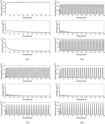
Firstly, for ${\mathcal{R}}_0<1$, using the parameter values (Table 2) results in ${\mathcal{R}}_0=0.5257$ and the dynamics given in Figure 1. For Figure 1(a–d), σ is varied to obtain a range of $C_0$ such that: (a) for $C_0=0.9921<1$ ($\sigma =0.0175$) it takes about 200 years for the infected resources to be eradicated, (b) for $C_0=1.2401>1$ ($\sigma =0.014$) it takes about 150 years for infected resources to be eradicated, (c) for $C_0=1.7361>1$ ($\sigma =0.010$) it takes about 100 years for infected resources to be eradicated, and (d) for $C_0=3.4722>1$ ($\sigma =0.0050$ ) it take about 50 years for infected resources to be eradicated. So, for ${\mathcal{R}}_0<1$ fixed, increasing $C_0$ results in faster eradication of the disease from the ecosystem.

Figure 1. Plot showing the possible long term dynamics for a fixed value of ${\mathcal{R}}_0=0.5257<1$ and various values of $C_0$ (see text for details). In each case, the disease is eradicated but as $C_0$ is increased this eradication is quicker. (a) $C_0=0.9921<1$. (b) $C_0=1.2401>1$. (c) $C_0=1.7361>1$. (d) $C_0=3.4722>1$.

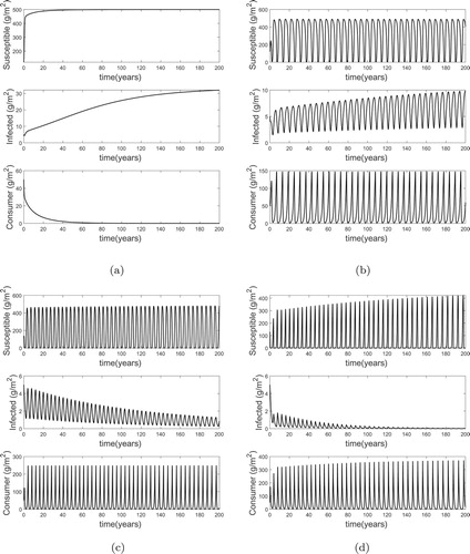
Secondly, for ${\mathcal{R}}_0>1$, again using the parameter values in Table 2, changing β results in ${\mathcal{R}}_0=2.1026$ and the dynamics given in Figure 2. Again, Figure 2(a–d) was obtained by varying σ to get a range of $C_0$ while keeping ${\mathcal{R}}_0=2.1026$ fixed. The results from Figure 2 are: (a) for $C_0=0.9921<1$ ($\sigma =0.0175$) the infected resources increase to a maximum biomass of about 30 g/m², (b) for $C_0=1.2401>1$ ($\sigma =0.014$) the infected resources increase to a maximum biomass of about 10 g/m², (c) for $C_0=1.7361>1$ ($\sigma =0.010$) the infected resources decrease to a minimum biomass of about 1.0 g/m², (d) for $C_0=3.4722>>1$ ($\sigma =0.0050$) the infected resources decrease to zero biomass (total eradication of infected population). Each of these dynamics occur over approximately 200 years except for the last one that is over a period of 100 years (Figure 2(d)).

Figure 2. Plot showing the possible long term dynamics for a fixed value of ${\mathcal{R}}_0=2.1026>1$ and various values of $C_0$ (see text for details). For $R_0>1$, the disease increases as expected as shown in (a) and (b). However, for greater values of $C_0$ the disease decreases (c) and if large enough can be eradicated (d). (a) $C_0=0.9921<1$. (b) $C_0=1.2401>1$. (c) $C_0=1.7361>1$. (d) $C_0=3.4722>1$.

3.3. Generalized model

To show how the results could be extended to more complex models we consider an ecosystem which consists of multiple patches with resources and consumers together with pathogens causing infectious diseases. We make the simplifying assumption that the disease is transmitted through direct contact with the pathogen and does not spread from one patch to another. Thus, while movement between and within patches is important, this is ignored. Also, the pathogen is assumed to affect each patch equally. Based on these assumptions we obtain the generalized model: (17) $\begin{array}{rl}\frac{\mathrm{d}{S}_1}{\mathrm{d}t}& =r_1{S}_1\left(1-\frac{S_1}{K_1}\right)-\frac{{\alpha }_1{Y}_1{S}_1}{{\rho }_1+S_1}-\frac{{\beta }_{1}P{S}_1}{\delta +P}+{\gamma }_1{I}_1,\\ \frac{\mathrm{d}{I}_1}{\mathrm{d}t}& =\frac{{\beta }_{1}P{S}_1}{\delta +P}-({\gamma }_1+{\mu }_1)I_1,\\ \frac{\mathrm{d}{Y}_1}{\mathrm{d}t}& =\frac{c_1{\alpha }_1{Y}_1{S}_1}{{\rho }_1+S_1}-{\sigma }_1{Y}_1,\\ & ⋮\\ \frac{\mathrm{d}{S}_n}{\mathrm{d}t}& =r_n{S}_n\left(1-\frac{S_n}{K_n}\right)-\frac{{\alpha }_n{Y}_n{S}_n}{{\rho }_n+S_n}-\frac{{\beta }_{n}P{S}_n}{\delta +P}+{\gamma }_n{I}_n,\\ \frac{\mathrm{d}{I}_n}{\mathrm{d}t}& =\frac{{\beta }_{n}P{S}_n}{\delta +P}-({\gamma }_n+{\mu }_n)I_n,\\ \frac{\mathrm{d}{Y}_n}{\mathrm{d}t}& =\frac{c_n{\alpha }_n{Y}_n{S}_n}{{\rho }_n+S_n}-{\sigma }_n{Y}_n,\\ \frac{\mathrm{d}P}{\mathrm{d}t}& ={\nu }_1{I}_1+{\nu }_2{I}_2+\cdots +{\nu }_n{I}_n-\xi P.\end{array}$(17) The meaning of variables and parameters are the same as given in Table 1 except for the subscript which represent the patch for the resources or consumer.

3.3.1. Generalized model: Preliminary analysis

The basic reproduction number ${\mathcal{R}}_0$ for the generalized model (17(17) $\begin{array}{rl}\frac{\mathrm{d}{S}_1}{\mathrm{d}t}& =r_1{S}_1\left(1-\frac{S_1}{K_1}\right)-\frac{{\alpha }_1{Y}_1{S}_1}{{\rho }_1+S_1}-\frac{{\beta }_{1}P{S}_1}{\delta +P}+{\gamma }_1{I}_1,\\ \frac{\mathrm{d}{I}_1}{\mathrm{d}t}& =\frac{{\beta }_{1}P{S}_1}{\delta +P}-({\gamma }_1+{\mu }_1)I_1,\\ \frac{\mathrm{d}{Y}_1}{\mathrm{d}t}& =\frac{c_1{\alpha }_1{Y}_1{S}_1}{{\rho }_1+S_1}-{\sigma }_1{Y}_1,\\ & ⋮\\ \frac{\mathrm{d}{S}_n}{\mathrm{d}t}& =r_n{S}_n\left(1-\frac{S_n}{K_n}\right)-\frac{{\alpha }_n{Y}_n{S}_n}{{\rho }_n+S_n}-\frac{{\beta }_{n}P{S}_n}{\delta +P}+{\gamma }_n{I}_n,\\ \frac{\mathrm{d}{I}_n}{\mathrm{d}t}& =\frac{{\beta }_{n}P{S}_n}{\delta +P}-({\gamma }_n+{\mu }_n)I_n,\\ \frac{\mathrm{d}{Y}_n}{\mathrm{d}t}& =\frac{c_n{\alpha }_n{Y}_n{S}_n}{{\rho }_n+S_n}-{\sigma }_n{Y}_n,\\ \frac{\mathrm{d}P}{\mathrm{d}t}& ={\nu }_1{I}_1+{\nu }_2{I}_2+\cdots +{\nu }_n{I}_n-\xi P.\end{array}$(17) ) is also computed using the next generation matrix method [46] and is (18) ${\mathcal{R}}_0=\sum _{i=1}^n{\mathcal{R}}_i,$(18) where ${\mathcal{R}}_i=\frac{{\beta }_i{\nu }_i{K}_i}{\delta \xi ({\gamma }_i+{\mu }_i)}$.

The consumption number $C_0$ for the generalized model (17(17) $\begin{array}{rl}\frac{\mathrm{d}{S}_1}{\mathrm{d}t}& =r_1{S}_1\left(1-\frac{S_1}{K_1}\right)-\frac{{\alpha }_1{Y}_1{S}_1}{{\rho }_1+S_1}-\frac{{\beta }_{1}P{S}_1}{\delta +P}+{\gamma }_1{I}_1,\\ \frac{\mathrm{d}{I}_1}{\mathrm{d}t}& =\frac{{\beta }_{1}P{S}_1}{\delta +P}-({\gamma }_1+{\mu }_1)I_1,\\ \frac{\mathrm{d}{Y}_1}{\mathrm{d}t}& =\frac{c_1{\alpha }_1{Y}_1{S}_1}{{\rho }_1+S_1}-{\sigma }_1{Y}_1,\\ & ⋮\\ \frac{\mathrm{d}{S}_n}{\mathrm{d}t}& =r_n{S}_n\left(1-\frac{S_n}{K_n}\right)-\frac{{\alpha }_n{Y}_n{S}_n}{{\rho }_n+S_n}-\frac{{\beta }_{n}P{S}_n}{\delta +P}+{\gamma }_n{I}_n,\\ \frac{\mathrm{d}{I}_n}{\mathrm{d}t}& =\frac{{\beta }_{n}P{S}_n}{\delta +P}-({\gamma }_n+{\mu }_n)I_n,\\ \frac{\mathrm{d}{Y}_n}{\mathrm{d}t}& =\frac{c_n{\alpha }_n{Y}_n{S}_n}{{\rho }_n+S_n}-{\sigma }_n{Y}_n,\\ \frac{\mathrm{d}P}{\mathrm{d}t}& ={\nu }_1{I}_1+{\nu }_2{I}_2+\cdots +{\nu }_n{I}_n-\xi P.\end{array}$(17) ) is also calculated using the approach in [13,46] and is (19) $C_0=max\left\{C_i\right\},i=1,2,\dots ,n,$(19) where $C_i=\frac{c_i{\alpha }_i{K}_i}{{\sigma }_i({\rho }_i+K_i)}$.

Thus, because the basic reproduction and the consumption numbers for this more general model can also be calculated it should also be possible to use them to investigate the system dynamics as illustrated using the simplified version of the model. This possibility needs further analyses and will be considered in future work.

4. Discussion

In summary, a consumer-resource model is presented here where resources are exposed to disease. The basic reproduction number and the consumption number are calculated and shown to govern the dynamics in agreement with fundamental results in the literature [8,13,17,44,46].

As explained is the introduction understanding the bifurcation dynamics at ${\mathcal{R}}_0=1$ can be important [6]. For our system we show that there is no backward bifurcation and so going through ${\mathcal{R}}_0=1$ in either direction does not affect the qualitative behaviour of the dynamics. We show that a Hopf bifurcation occurs for a prescribed combination of parameter values and so cyclic dynamics are possible as found in other epidemiological models [4,10,26]. These cycles can be important as they can create further cyclical dynamics in the disease itself [9,28]. Also, if species densities are cycling then they can be vulnerable to environmental stochasticity [20].

It is well known in epidemiology that when the basic reproduction number is less than unity there is a greater chance of eradicating a disease. Using our model we show that forward bifurcation is possible and the disease is eradicated when ${\mathcal{R}}_0<1$ as expected [8,44,46]. However, we also show here that increasing the consumption number $C_0$ results in faster eradication of the disease from the system. Thus, increasing the strength of coexistence between the consumer and the resources results in faster disease elimination. As far as we know this effect on the rate of disease elimination has not been demonstrated previously and could be important in situations where stochastic events prevent elimination if the process is slow [21].

When ${\mathcal{R}}_0>1$, the model can show disease persistence, as expected. However, here we show that consumers can change this result. In fact, mathematical analyses and numerical examples show how with consumers present even with ${\mathcal{R}}_0>1$ the disease can be eradicated for some $C_0$ large enough. As explained in the introduction, larger values of $C_0$ will improve the likelihood of coexistence of resources and consumers. These results suggest an association between strengthening the coexistence of species and the eradication of certain diseases from a system. This association highlights the possible importance of future research on the extent to which interventions that support coexistence might reduce the spread of infectious diseases (including the prevalence and consequences of such diseases). Moreover, if future research indicted a causal relation between species coexistence and disease prevalence then a possible consequence could be that consumer extinction (through external factors) would increase diseases, further intensifying pressure on plant diversity as well.

One possible mechanism for this type of process is that consumption eliminates infectious individuals thus preventing the spread of disease [25,39]. Also, in a predator prey situation this process can be exacerbated by the possible weakening of prey by disease making them more vulnerable to predation [25].

Infectious diseases in natural resources are common and inevitable. This study provides epidemiological reproduction and consumption numbers for understanding how such a disease might operate in a consumer resource system. These are biologically conceivable quantities and in principle could be measured [26]. Thus, field studies together with the models could be used to predict disease progression. For example, for a particular ecosystem, field estimates for variables such as carrying capacity, conversion and consumption rates of resource to consumer biomass, and the other variables that constitute $C_0$ could be used together with measures of the parameters in ${\mathcal{R}}_0$ to determine the possible disease dynamics. In particular, eradication or not of the disease can then be assessed. The resilience of the ecosystem can then be explored under scenarios of pressure from factors such climatic variability, human settlement or poaching. Also, if it is ascertained that consumers (predators or herbivores) are important for disease dynamics this knowledge could be important when managing culling or hunting programmes.

The original model described here is simple but gives the fundamental characteristics of possible consumer-resource systems. However, it still displays complex behaviour and its simplicity allows a more complete analysis [20]. Many possible extensions can be used to effectively describe actual situations. We use one example of a more complex model, with multiple patches and consumers, resources and disease, and the same results are likely to hold. Also, this model is made with a particular set of assumptions that could be altered to better suit specific ”real world” systems, and these alternative models could be worth pursuing in future research efforts.

It is understood to a certain extent that in ecosystems the occurrence of infectious diseases can have a negative effect in reducing ecosystem sustainability by affecting the coexistence of species. Alternatively, it has been shown that ecosystem biodiversity can affect disease transmission rates [30]. Thus, it appears that ecosystem sustainability could affect levels of infections diseases. Here we show how coexistence of consumers and their resources could contribute to reduced levels of disease. This possibility could be important for more complicated systems and the overall persistence of ecosystems. A further advantage is that if disease is reduced in natural systems then this could also reduce infections in domesticated species in which there is contact, such as food crops, with possible economic and public health cost benefits [24]. Lastly, if incidences of disease increase as consumers are driven extinct then eventual declines in resource diversity are also a possible consequence.

Disclosure statement

No potential conflict of interest was reported by the authors.

Additional information

Funding

This work was supported in part by an African Union Research (supported by the European Union) [grant number AURG/090/2012] and the South African Department of Science and Technology.

References

- R.M. Anderson and R.M. May, The population dynamics of microparasites and their invertebrate hosts, Phil. Trans. R. Soc. Lond. B 291(1054) (1981), pp. 451–524.
- P. Auger, R. Mchich, T. Chowdhury, G. Sallet, M. Tchuente, and J. Chattopadhyay, Effects of a disease affecting a predator on the dynamics of a predator–prey system, J. Theor. Biol. 258(3) (2009), pp. 344–351.
- M. Barfield, M. Martcheva, N. Tuncer, and R.D. Holt, Backward bifurcation and oscillations in a nested immuno-eco-epidemiological model, J. Biol. Dyn. 12(1) (2018), pp. 51–88.
- A.M. Bate and F.M. Hilker, Complex dynamics in an eco-epidemiological model, Bull Math. Biol.75(11) (2013), pp. 2059–2078.
- F. Brauer, Backward bifurcations in simple vaccination models, J. Math. Anal. Appl. 298(2) (2004), pp. 418–431.
- F. Brauer, Mathematical epidemiology: Past, present, and future, Infect. Dis. Model. 2(2) (2017), pp. 113–127.
- C. Castillo-Chavez, K. Cooke, W. Huang, and S.A. Levin, Results on the dynamics for models for the sexual transmission of the human immunodeficiency virus, Appl. Math. Lett. 2(4) (1989), pp. 327–331.
- C. Castillo-Chavez, Z. Feng, and W. Huang, On the computation of R0 and its role on global stability in Mathematical Approaches for Emerging and Re-emerging Infectious Diseases: An Introduction, IMA 125, Springer-Verlag; 2002
- R.D. Cavanagh, X. Lambin, T. Ergon, M. Bennett, I.M. Graham, D. van Soolingen, and M. Begon, Disease dynamics in cyclic populations of field voles (Microtus agrestis): Cowpox virus and vole tuberculosis (Mycobacterium microti), Proc. R. Soc. B Biol. Sci. 271(1541) (2004), pp. 859–867.
- S. Chakraborty, B.W. Kooi, B. Biswas, and J. Chattopadhyay, Revealing the role of predator interference in a predatorprey system with disease in prey population, Ecol. Complex. 21 (2015), pp. 100–111.
- J. Chattopadhyay and O. Arino, A predator-prey model with disease in the prey, Nonlinear Anal. Theory Methods Appl. 36 (6), (1999), pp. 747–766.
- C.T. Codeo, Endemic and epidemic dynamics of cholera: The role of the aquatic reservoir, BMC Infectious Diseases 1 (1), (2001), pp. 209.
- O.C. Collins and K.J. Duffy, Consumption threshold used to investigate stability and ecological dominance in consumer-resource dynamics, Ecol. Model. 319 (2016), pp. 155–162.
- O.C. Collins and K.J. Duffy, Optimal control of maize foliar diseases using the plants population dynamics, Acta Agric. Scand B Soil Plant Sci. 66 (2016), pp. 20–26.
- P. Daszak, A.A. Cunningham, and A.D. Hyatt, Emerging infectious diseases of wildlife–threats to biodiversity and human health, Science 287 (2000), pp. 443–449.
- K.J. Duffy, Simulations to investigate animal movement effects on population, Nat. Resour. Model.24 (2001), pp. 48–60.
- K.J. Duffy and O.C Collins, Identifying stability conditions and Hopf bifurcations in a consumer resource model using a consumption threshold, Ecol. Complex. 28 (2016), pp. 212–217.
- M.A. Duffy, J.M. Housley, R.M. Penczykowski, C.E. Caceres, and S.E. Hall, Unhealthy herds: Indirect effects of predators enhance two drivers of disease spread, Funct. Ecol. 25(5) (2011), pp. 945–953.
- J. Dushoff, W. Huang, and C. Castillo-Chavez, Backwards bifurcations and catastrophe in simple models of fatal diseases, J. Math. Biol. 36(3) (1998), pp. 227–248.
- J.M. Fryxell, C. Packer, K. McCann, E.J. Solberg, and B-E. Sther, Resource management cycles and the sustainability of harvested wildlife populations, Science 328 (5980), (2010), pp. 903–906.
- S. Greenhalgh, A.P. Galvani, and J. Medlock, Disease elimination and re-emergence in differential-equation models, J. Theor. Biol. 387 (2015), pp. 174–180.
- A.B. Gumel, Causes of backward bifurcations in some epidemiological models, J. Math. Anal. Appl.395(1) (2012), pp. 355–365.
- M. Haque and E. Venturino, The role of transmissible diseases in the Holling-Tanner predator-prey model, Theor. Popul. Biol. 70(3) (2006), pp. 273–288.
- M.J. Hatcher, J.T. Dick, and A.M. Dunn, How parasites affect interactions between competitors and predators, Ecol. Lett. 9 (11), (2006), pp. 1253–1271.
- H.W. Hethcote, W. Wang, L. Han, and Z. Ma, A predatorprey model with infected prey, Theor. Popul. Biol. 66(3) (2004), pp. 259–268.
- F.M. Hilker and K. Schmitz, Disease-induced stabilization of predator-prey oscillations, J. Theor. Biol.255(3) (2008), pp. 299–306.
- R.D. Holt and M. Roy, Predation can increase the prevalence of infectious diseases, Am. Nat. 169(5) (2007), pp. 690–699.
- P.J. Hurtado, S.R. Hall, and S.P. Ellner, Infectious disease in consumer populations: Dynamic consequences of resource-mediated transmission and infectiousness, Theor. Ecol. 7 (2014), pp. 163–179.
- P.T. Johnson, D.L. Preston, J.T. Hoverman, and K.L. Richgels, Biodiversity decreases disease through predictable changes in host community competence, Nature 494 (2013), pp. 230–233.
- F. Keesing, L.K. Belden, P. Daszak, A. Dobson, C.D. Harvell, R.D. Holt, P. Hudson, A. Jolles, K.E.Jones, C.E. Mitchell, and S.S. Myers, Impacts of biodiversity on the emergence and transmission of infectious diseases, Nature 468 (2010), pp. 647–652.
- B.W. Kooi, G.A.K. van Voorn, and K. pada Das, Stabilisation and complex dynamics in a predator-prey model with predator suffering from an infectious disease, Ecol. Complex. 8 (2011), pp. 113–122.
- B.W. Kooi and E. Venturino, Ecoepidemic predator–prey model with feeding satiation, prey herd behavior and abandoned infected prey, Math. Biosci. 274 (2016), pp. 58–72.
- S. Liao and J. Wang, Stability analysis and application of a mathematical cholera model, Math. Biosci. Eng. 8 (2011), pp. 733–752.
- H. McCallum, N. Barlow, and J. Hone, How should pathogen transmission be modelled?, Trends Ecol. Evol. 16(6) (2001), pp. 295–300.
- Z. Mukandavire, S. Liao, J. Wang, H. Gaff, D.L. Smith, and J.G. Morris, Estimating the reproductive numbers for the 2008–2009 cholera outbreaks in Zimbabwe, Proc. R. Acad. Sci. 108 (21), (2011), pp. 8767–8772.
- T. Nakazawa, T. Yamanaka, and S. Urano, Model analysis for plant disease dynamics co-mediated by herbivory and herbivore-borne phytopathogens, Biol. Lett. 8 (2012), pp. 685–688.
- N. Chitnis, J.M. Cushing, J.M. Hyman, Bifurcation analysis of a mathematical model for malaria transmission. SIAM J. Appl. Math. 67(1) (2006), pp. 24–45.
- N. Owen-Smith, Functional heterogeneity in resources within landscapes and herbivore population dynamics, Landscape Ecol. 19 (2004), pp. 761–771.
- C. Packer, R.D. Holt, P.J. Hudson, K.D. Lafferty, and A.P. Dobson, Keeping the herds healthy and alert: Implications of predator control for infectious disease, Ecol. Lett. 6(9) (2003), pp. 797–802.
- K. Pada Das, K. Kundu, and J.A. Chattopadhyay, A predator-prey mathematical model with both the populations affected by diseases, Ecol. Complex. 8 (2011), pp. 68–80.
- A.H. Robbins, M.D. Borden, B.S. Windmiller, M. Niezgoda, L.C. Marcus, S.M. O'Brien, S.M. Kreindel, M.W. McGuill, A. DeMariaJr, C.E. Rupprecht, and S. Rowell, Prevention of the spread of rabies to wildlife by oral vaccination of raccoons in Massachusetts, J. Am. Vet. Med. Assoc. 213(10) (1998), pp. 1407–1412.
- R. Ross, The Prevention of Malaria, 2nd ed. John Murray, London, UK, 1911.
- J.J. Tewa, V.Y. Djeumen, and S. Bowong, Predator-prey model with Holling response function of type II and SIS infectious disease, Appl. Math. Model. 37 (2013), pp. 4825–4841.
- J.H. Tien and D.J.D. Earn, Multiple transmission pathways and disease dynamics in a waterborne pathogen model, Bull. Math. Biol. 72 (2010), pp. 1506–1533.
- P. Turchin, Complex Population Dynamics: A Theoretical/Empirical Synthesis, Princeton University Press, Princeton, NJ, 2003.
- P. van den Driessche and J. Watmough, Reproduction numbers and sub-threshold endemic equilibria for compartmental models of disease transmission, Math. Biosci. 180 (2002), pp. 29–48.
- E. Venturino, Ecoepidemiology: a more comprehensive view of population interactions, Math. Model Nat. Phenom. 11(1) (2016), pp. 49–90.