Global dynamics of a tuberculosis model with fast and slow progression and age-dependent latency and infection

ABSTRACT

In this paper, a mathematical model describing tuberculosis transmission with fast and slow progression and age-dependent latency and infection is investigated. It is assumed in the model that infected individuals can develop tuberculosis by either of two pathogenic mechanisms: direct progression or endogenous reactivation. It is shown that the transmission dynamics of the disease is fully determined by the basic reproduction number. By analyzing corresponding characteristic equations, the local stability of a disease-free steady state and an endemic steady state of the model is established. By using the persistence theory for infinite dimensional system, it is proved that the system is uniformly persistent when the basic reproduction number is greater than unity. By constructing suitable Lyapunov functionals and using LaSalle's invariance principle, it is verified that the global dynamics of the system is completely determined by the basic reproduction number.

KEYWORDS:

• Tuberculosis
• fast and slow progression
• age-dependent latency and infection
• stability
• Lyapunov functional

2000 MATHEMATICS SUBJECT CLASSIFICATIONS:

• 37N25
• 92B05
• 37B25

View correction statement:

Correction

1. Introduction

Tuberculosis (TB) is a bacterial disease caused by Mycobacterium tuberculosis, and is usually acquired through airborne infection from active TB cases [4,9]. According to the World Health Organization, one third of the world's population is infected with tuberculosis either latently or actively. Despite effective antimicrobial chemotherapy, tuberculosis infection remains a leading cause of death from an infectious disease [34].

Mathematical modelling has been proven to be important in better understanding the transmission dynamics of TB and evaluating the effectiveness of various control and prevention strategies (see, for example, [1–3,5–7,10–12,18–21,25,29,30,32]). Tuberculosis is most commonly transmitted from a person suffering from infectious (active) tuberculosis to other persons by infected droplets created when the person with active TB coughs or sneezes. Among generally healthy persons, infection with TB is highly likely to be asymptomatic [10]. In [6], Blower et al. formulated and analysed mathematical models describing the transmission dynamics of untreated tuberculosis epidemics. It was assumed in [6] that infected individuals remain noninfectious until they develop disease by one of two pathogenic mechanisms: direct progression or endogenous reactivation. Two types of tuberculosis contribute to the incidence rate of tuberculosis disease: one type of tuberculosis develops through direct progression soon after infection (fast progression) and the other type of tuberculosis develops through endogenous reactivation in the latently infected individuals (slow progression). In order to assess the intrinsic transmission dynamics of tuberculosis, Blower et al. considered the following mathematical model [6]: (1) $\begin{array}{rl}\dot{S}(t)& =A-\mu S(t)-\beta S(t)I(t),\\ \dot{L}(t)& =(1-p)\beta S(t)I(t)-\nu L(t)-\mu L(t),\\ \dot{I}(t)& =p\beta S(t)I(t)+\nu L(t)-(\mu +{\mu }_T)I(t).\end{array}$(1) In (1(1) $\begin{array}{rl}\dot{S}(t)& =A-\mu S(t)-\beta S(t)I(t),\\ \dot{L}(t)& =(1-p)\beta S(t)I(t)-\nu L(t)-\mu L(t),\\ \dot{I}(t)& =p\beta S(t)I(t)+\nu L(t)-(\mu +{\mu }_T)I(t).\end{array}$(1) ), $S(t)$ represents the number of individuals who are not previously exposed to tuberculosis at time t, $L(t)$ represents the number of latently infected individuals who have been infected with Mycobacterium tuberculosis at time t, but have no clinical illness and remain noninfectious, $I(t)$ represents the number of active infectious tuberculosis cases at time t. The assumptions of model (1(1) $\begin{array}{rl}\dot{S}(t)& =A-\mu S(t)-\beta S(t)I(t),\\ \dot{L}(t)& =(1-p)\beta S(t)I(t)-\nu L(t)-\mu L(t),\\ \dot{I}(t)& =p\beta S(t)I(t)+\nu L(t)-(\mu +{\mu }_T)I(t).\end{array}$(1) ) were made as follows [6].

1. Recruitment to the susceptible population occurs at a constant rate A. The incidence rate of infection is formulated as the product of the number of susceptible population at time t and the per capita force of infection at time t, where the per capita infection force is defined as the per-susceptible risk of becoming infected with Mycobacterium tuberculosis, and is calculated as the product of the number of infectious cases at time t and the transmission coefficient (β) of the pathogen. Where β represents the likelihood that an infectious case will successfully transmit the infection to a susceptible individual.

2. The two pathogenous mechanisms are assumed by allowing a proportion (p) of the newly infected to develop tuberculosis directly and a proportion (1−p) of the newly infected to enter the latent class. Latently infected individuals either develop tuberculosis slowly at an average rate ν or die at a natural death rate μ before developing tuberculosis.

3. Active infectious tuberculosis die, either because of tuberculosis at average rate ${\mu }_T$, or because of natural death at an average rate μ.

The qualitative dynamics of model (1(1) $\begin{array}{rl}\dot{S}(t)& =A-\mu S(t)-\beta S(t)I(t),\\ \dot{L}(t)& =(1-p)\beta S(t)I(t)-\nu L(t)-\mu L(t),\\ \dot{I}(t)& =p\beta S(t)I(t)+\nu L(t)-(\mu +{\mu }_T)I(t).\end{array}$(1) ) are governed by the basic reproduction number: (2) ${\mathcal{R}}_0=p{\displaystyle \frac{A\beta }{\mu (\mu +{\mu }_T)}+(1-p){\displaystyle \frac{A\beta \nu }{\mu (\mu +{\mu }_T)(\mu +\nu )}.}}$(2) Where the quantity ${\mathcal{R}}_0$ represents the average number of secondary infectious cases produced by a typical infectious individual in a susceptible population at a demographic steady state. The first term in (2(2) ${\mathcal{R}}_0=p{\displaystyle \frac{A\beta }{\mu (\mu +{\mu }_T)}+(1-p){\displaystyle \frac{A\beta \nu }{\mu (\mu +{\mu }_T)(\mu +\nu )}.}}$(2) ) gives the new cases resulting from fast progression while the second term represents the cases resulting from slow progression.

We note that system (1(1) $\begin{array}{rl}\dot{S}(t)& =A-\mu S(t)-\beta S(t)I(t),\\ \dot{L}(t)& =(1-p)\beta S(t)I(t)-\nu L(t)-\mu L(t),\\ \dot{I}(t)& =p\beta S(t)I(t)+\nu L(t)-(\mu +{\mu }_T)I(t).\end{array}$(1) ) was formulated as ordinary differential equations with distinct variables describing the population size of compartments such as susceptible, latently infected and active infectious. It is assumed that all individuals within a compartment behave identically, regardless of how much time they have spent in the compartment. However, an infected individuals may have latent tuberculosis for months, years or even decades before the disease becomes infectious. The risk per unit time of activation appears to be higher in the early stages of latency than in later stages [6]. On the other hand, laboratory studies suggest that the infectivity of infectious individuals be different at the differential age of infection [39]. For tuberculosis infection, the TB bacteria need to develop in the lung to be transmissible through coughing, and their transmissibility depends on their progression in the lung as well as the strength of a host's immune system. Active TB has the highest possibility of developing within the first 2–5 years of infection, while most TB infections remain latent for a long period of time until immune compromise occurs due to aging or co-infection with other illnesses such as HIV (see, for example, [14,25]). In [28], by including the duration that an individual has spent in the exposed compartment and in the infectious compartment as variables, McCluskey presented and studied an SEI epidemiological model with continuous age-structure in the exposed and infectious classes. A Lyapunov functional was used in [28] to show that the endemic steady state is globally stable. Recently, much attention has been paid to the modelling and analysis on infectious disease dynamics with age dependence (see, for example, [8,13,15–17,27,36]).

Motivated by the works of Blower et al. [6] and McCluskey [28], in the present paper, we are concerned with the effect of age structure for both latently infected and active infectious individuals on the transmission dynamics of untreated tuberculosis epidemics with fast and slow progression. To this end, we consider the following differential equation system: (3) $\begin{array}{rl}\dot{S}(t)& =A-{\mu }_{S}S(t)-S(t){\int }_0^{\mathrm{\infty }}\beta (a)i(a,t)\mathrm{d}a,\\ {\displaystyle \frac{\mathrm{\partial }e(\theta ,t)}{\mathrm{\partial }t}+{\displaystyle \frac{\mathrm{\partial }e(\theta ,t)}{\mathrm{\partial }\theta }}}& =-(\mu (\theta )+\epsilon (\theta ))e(\theta ,t),\theta >0,\\ {\displaystyle \frac{\mathrm{\partial }i(a,t)}{\mathrm{\partial }t}+{\displaystyle \frac{\mathrm{\partial }i(a,t)}{\mathrm{\partial }a}}}& =-\nu (a)i(a,t),a>0\end{array}$(3) with boundary conditions (4) $\begin{array}{rl}e(0,t)& =(1-p)S(t){\int }_0^{\mathrm{\infty }}\beta (a)i(a,t)\mathrm{d}a,\\ i(0,t)& =pS(t){\int }_0^{\mathrm{\infty }}\beta (a)i(a,t)\mathrm{d}a+{\int }_0^{\mathrm{\infty }}\epsilon (\theta )e(\theta ,t)\mathrm{d}\theta ,\end{array}$(4) and initial condition (5) $X_0:=(S(0),e(\cdot ,0),i(\cdot ,0))=(S^0,e_0(\cdot ),i_0(\cdot ))\in \mathcal{X},$(5) where $\mathcal{X}={\mathbb{R}}^{+}\times L_{+}^1(0,\mathrm{\infty })\times L_{+}^1(0,\mathrm{\infty })$, $L_{+}^1(0,\mathrm{\infty })$ is the set of all integrable functions from $(0,\mathrm{\infty })$ into ${\mathbb{R}}^{+}=[0,\mathrm{\infty })$.

In system (3(3) $\begin{array}{rl}\dot{S}(t)& =A-{\mu }_{S}S(t)-S(t){\int }_0^{\mathrm{\infty }}\beta (a)i(a,t)\mathrm{d}a,\\ {\displaystyle \frac{\mathrm{\partial }e(\theta ,t)}{\mathrm{\partial }t}+{\displaystyle \frac{\mathrm{\partial }e(\theta ,t)}{\mathrm{\partial }\theta }}}& =-(\mu (\theta )+\epsilon (\theta ))e(\theta ,t),\theta >0,\\ {\displaystyle \frac{\mathrm{\partial }i(a,t)}{\mathrm{\partial }t}+{\displaystyle \frac{\mathrm{\partial }i(a,t)}{\mathrm{\partial }a}}}& =-\nu (a)i(a,t),a>0\end{array}$(3) ), $S(t)$ represents the number of individuals who are susceptible to tuberculosis at time t; $e(\theta ,t)$ represents the density of individuals who have been in the latently infected class for duration θ at time t, but have no clinical illness and remain noninfectious; $i(a,t)$ represents the density of individuals who have been in the active infectious class for duration a at time t. The definitions of all parameters and symbols in system (3(3) $\begin{array}{rl}\dot{S}(t)& =A-{\mu }_{S}S(t)-S(t){\int }_0^{\mathrm{\infty }}\beta (a)i(a,t)\mathrm{d}a,\\ {\displaystyle \frac{\mathrm{\partial }e(\theta ,t)}{\mathrm{\partial }t}+{\displaystyle \frac{\mathrm{\partial }e(\theta ,t)}{\mathrm{\partial }\theta }}}& =-(\mu (\theta )+\epsilon (\theta ))e(\theta ,t),\theta >0,\\ {\displaystyle \frac{\mathrm{\partial }i(a,t)}{\mathrm{\partial }t}+{\displaystyle \frac{\mathrm{\partial }i(a,t)}{\mathrm{\partial }a}}}& =-\nu (a)i(a,t),a>0\end{array}$(3) ) are listed in Table 1.

Table 1. Definitions of the parameters and symbols in the system (3(3) $\begin{array}{rl}\dot{S}(t)& =A-{\mu }_{S}S(t)-S(t){\int }_0^{\mathrm{\infty }}\beta (a)i(a,t)\mathrm{d}a,\\ {\displaystyle \frac{\mathrm{\partial }e(\theta ,t)}{\mathrm{\partial }t}+{\displaystyle \frac{\mathrm{\partial }e(\theta ,t)}{\mathrm{\partial }\theta }}}& =-(\mu (\theta )+\epsilon (\theta ))e(\theta ,t),\theta >0,\\ {\displaystyle \frac{\mathrm{\partial }i(a,t)}{\mathrm{\partial }t}+{\displaystyle \frac{\mathrm{\partial }i(a,t)}{\mathrm{\partial }a}}}& =-\nu (a)i(a,t),a>0\end{array}$(3) ).

Parameters	Description
A	The recruitment rate
${\mu }_S$	Per capita natural death rate of the susceptible population
θ	The duration for which individuals have been in the latently infected class
a	Age of infection, i.e. the time that has lapsed since the individual became infectious
$\mu (\theta )$	The rate at which individuals who have been in the latently infected class for duration θ are removed
$\epsilon (\theta )$	The rate at which individuals who have been in the latently infected class for duration θ progress to the active infectious class
$\beta (a)$	The transmission coefficient of active infectious individuals at age of infection a
$\nu (a)$	The natural and disease-induced death rate of individuals who have been in the active infectious class for duration a
p	The proportion of the newly infected to develop tuberculosis directly
1−p	The proportion of the newly infected to enter the latent class

In the sequel, we further make the following assumptions.

1. β and ϵ are Lipschitz continuous on ${\mathbb{R}}^{+}$ with Lipschitz coefficients $L_{\beta }$ and $L_{\epsilon }$, respectively.

2. $\beta ,\epsilon ,\mu ,\nu \in L_{+}^{\mathrm{\infty }}(0,\mathrm{\infty })$ with essential upper bounds $\overline{\beta },\overline{\epsilon },\overline{\mu }$ and $\overline{\nu }$, respectively.

3. There exists ${\mu }_0\in (0,{\mu }_S]$ such that $\mu (a)\ge {\mu }_0$ for $a\ge 0$ and $\nu (\theta )\ge {\mu }_0$ for $\theta \ge 0$.

4. There exist positive constants $a_{\beta }$ and $a_{\epsilon }$ such that $\beta (a)$ is positive in a neighbourhood of $a_{\beta }$ and $\epsilon (a)$ is positive in a neighbourhood of $a_{\epsilon }$.

Using the theory of age-structured dynamical systems developed in [24,35], we can show that system (3(3) $\begin{array}{rl}\dot{S}(t)& =A-{\mu }_{S}S(t)-S(t){\int }_0^{\mathrm{\infty }}\beta (a)i(a,t)\mathrm{d}a,\\ {\displaystyle \frac{\mathrm{\partial }e(\theta ,t)}{\mathrm{\partial }t}+{\displaystyle \frac{\mathrm{\partial }e(\theta ,t)}{\mathrm{\partial }\theta }}}& =-(\mu (\theta )+\epsilon (\theta ))e(\theta ,t),\theta >0,\\ {\displaystyle \frac{\mathrm{\partial }i(a,t)}{\mathrm{\partial }t}+{\displaystyle \frac{\mathrm{\partial }i(a,t)}{\mathrm{\partial }a}}}& =-\nu (a)i(a,t),a>0\end{array}$(3) ) has a unique solution $(S(t),e(\cdot ,t),i(\cdot ,t))$ satisfying the boundary conditions (4(4) $\begin{array}{rl}e(0,t)& =(1-p)S(t){\int }_0^{\mathrm{\infty }}\beta (a)i(a,t)\mathrm{d}a,\\ i(0,t)& =pS(t){\int }_0^{\mathrm{\infty }}\beta (a)i(a,t)\mathrm{d}a+{\int }_0^{\mathrm{\infty }}\epsilon (\theta )e(\theta ,t)\mathrm{d}\theta ,\end{array}$(4) ) and the initial condition (5(5) $X_0:=(S(0),e(\cdot ,0),i(\cdot ,0))=(S^0,e_0(\cdot ),i_0(\cdot ))\in \mathcal{X},$(5) ). Moreover, it is easy to show that all solutions of system (3(3) $\begin{array}{rl}\dot{S}(t)& =A-{\mu }_{S}S(t)-S(t){\int }_0^{\mathrm{\infty }}\beta (a)i(a,t)\mathrm{d}a,\\ {\displaystyle \frac{\mathrm{\partial }e(\theta ,t)}{\mathrm{\partial }t}+{\displaystyle \frac{\mathrm{\partial }e(\theta ,t)}{\mathrm{\partial }\theta }}}& =-(\mu (\theta )+\epsilon (\theta ))e(\theta ,t),\theta >0,\\ {\displaystyle \frac{\mathrm{\partial }i(a,t)}{\mathrm{\partial }t}+{\displaystyle \frac{\mathrm{\partial }i(a,t)}{\mathrm{\partial }a}}}& =-\nu (a)i(a,t),a>0\end{array}$(3) ) with the boundary conditions (4(4) $\begin{array}{rl}e(0,t)& =(1-p)S(t){\int }_0^{\mathrm{\infty }}\beta (a)i(a,t)\mathrm{d}a,\\ i(0,t)& =pS(t){\int }_0^{\mathrm{\infty }}\beta (a)i(a,t)\mathrm{d}a+{\int }_0^{\mathrm{\infty }}\epsilon (\theta )e(\theta ,t)\mathrm{d}\theta ,\end{array}$(4) ) and the initial condition (5(5) $X_0:=(S(0),e(\cdot ,0),i(\cdot ,0))=(S^0,e_0(\cdot ),i_0(\cdot ))\in \mathcal{X},$(5) ) are defined on $[0,+\mathrm{\infty })$ and remain positive for all $t\ge 0$. Furthermore, $\mathcal{X}$ is positively invariant and system (3(3) $\begin{array}{rl}\dot{S}(t)& =A-{\mu }_{S}S(t)-S(t){\int }_0^{\mathrm{\infty }}\beta (a)i(a,t)\mathrm{d}a,\\ {\displaystyle \frac{\mathrm{\partial }e(\theta ,t)}{\mathrm{\partial }t}+{\displaystyle \frac{\mathrm{\partial }e(\theta ,t)}{\mathrm{\partial }\theta }}}& =-(\mu (\theta )+\epsilon (\theta ))e(\theta ,t),\theta >0,\\ {\displaystyle \frac{\mathrm{\partial }i(a,t)}{\mathrm{\partial }t}+{\displaystyle \frac{\mathrm{\partial }i(a,t)}{\mathrm{\partial }a}}}& =-\nu (a)i(a,t),a>0\end{array}$(3) ) exhibits a continuous semi-flow $\mathrm{\Phi }:{\mathbb{R}}^{+}\times \mathcal{X}\to \mathcal{X}$, namely, (6) ${\mathrm{\Phi }}_t(X_0)=\mathrm{\Phi }(t,X_0):=(S(t),e(\cdot ,t),i(\cdot ,t)),t\ge 0,X_0\in \mathcal{X}.$(6)

Given a point $(x,\phi ,\psi )\in \mathcal{X}$, we have the norm $\Vert (x,\phi ,\psi ){\Vert }_{\mathcal{X}}:=x+{\int }_0^{\mathrm{\infty }}\phi (a)\mathrm{d}a+{\int }_0^{\mathrm{\infty }}\psi (\theta )\mathrm{d}\theta .$

The primary goal of the present work is to carry out a complete mathematical analysis of system (3(3) $\begin{array}{rl}\dot{S}(t)& =A-{\mu }_{S}S(t)-S(t){\int }_0^{\mathrm{\infty }}\beta (a)i(a,t)\mathrm{d}a,\\ {\displaystyle \frac{\mathrm{\partial }e(\theta ,t)}{\mathrm{\partial }t}+{\displaystyle \frac{\mathrm{\partial }e(\theta ,t)}{\mathrm{\partial }\theta }}}& =-(\mu (\theta )+\epsilon (\theta ))e(\theta ,t),\theta >0,\\ {\displaystyle \frac{\mathrm{\partial }i(a,t)}{\mathrm{\partial }t}+{\displaystyle \frac{\mathrm{\partial }i(a,t)}{\mathrm{\partial }a}}}& =-\nu (a)i(a,t),a>0\end{array}$(3) ) with the boundary conditions (4(4) $\begin{array}{rl}e(0,t)& =(1-p)S(t){\int }_0^{\mathrm{\infty }}\beta (a)i(a,t)\mathrm{d}a,\\ i(0,t)& =pS(t){\int }_0^{\mathrm{\infty }}\beta (a)i(a,t)\mathrm{d}a+{\int }_0^{\mathrm{\infty }}\epsilon (\theta )e(\theta ,t)\mathrm{d}\theta ,\end{array}$(4) ) and the initial condition (5(5) $X_0:=(S(0),e(\cdot ,0),i(\cdot ,0))=(S^0,e_0(\cdot ),i_0(\cdot ))\in \mathcal{X},$(5) ), and establish its global dynamics. The organization of this paper is as follows. In the next section, we show the asymptotic smoothness of the semi-flow generated by system (3(3) $\begin{array}{rl}\dot{S}(t)& =A-{\mu }_{S}S(t)-S(t){\int }_0^{\mathrm{\infty }}\beta (a)i(a,t)\mathrm{d}a,\\ {\displaystyle \frac{\mathrm{\partial }e(\theta ,t)}{\mathrm{\partial }t}+{\displaystyle \frac{\mathrm{\partial }e(\theta ,t)}{\mathrm{\partial }\theta }}}& =-(\mu (\theta )+\epsilon (\theta ))e(\theta ,t),\theta >0,\\ {\displaystyle \frac{\mathrm{\partial }i(a,t)}{\mathrm{\partial }t}+{\displaystyle \frac{\mathrm{\partial }i(a,t)}{\mathrm{\partial }a}}}& =-\nu (a)i(a,t),a>0\end{array}$(3) ). In Section 3, we calculate the basic reproduction number and discuss the existence of feasible steady states of system (3(3) $\begin{array}{rl}\dot{S}(t)& =A-{\mu }_{S}S(t)-S(t){\int }_0^{\mathrm{\infty }}\beta (a)i(a,t)\mathrm{d}a,\\ {\displaystyle \frac{\mathrm{\partial }e(\theta ,t)}{\mathrm{\partial }t}+{\displaystyle \frac{\mathrm{\partial }e(\theta ,t)}{\mathrm{\partial }\theta }}}& =-(\mu (\theta )+\epsilon (\theta ))e(\theta ,t),\theta >0,\\ {\displaystyle \frac{\mathrm{\partial }i(a,t)}{\mathrm{\partial }t}+{\displaystyle \frac{\mathrm{\partial }i(a,t)}{\mathrm{\partial }a}}}& =-\nu (a)i(a,t),a>0\end{array}$(3) ). In Section 4, by analyzing corresponding characteristic equations, we establish the local asymptotic stability of a disease-free steady state and an endemic steady state of system (3(3) $\begin{array}{rl}\dot{S}(t)& =A-{\mu }_{S}S(t)-S(t){\int }_0^{\mathrm{\infty }}\beta (a)i(a,t)\mathrm{d}a,\\ {\displaystyle \frac{\mathrm{\partial }e(\theta ,t)}{\mathrm{\partial }t}+{\displaystyle \frac{\mathrm{\partial }e(\theta ,t)}{\mathrm{\partial }\theta }}}& =-(\mu (\theta )+\epsilon (\theta ))e(\theta ,t),\theta >0,\\ {\displaystyle \frac{\mathrm{\partial }i(a,t)}{\mathrm{\partial }t}+{\displaystyle \frac{\mathrm{\partial }i(a,t)}{\mathrm{\partial }a}}}& =-\nu (a)i(a,t),a>0\end{array}$(3) ). In Section 5, by means of the persistence theory for infinite dimensional system, we show that system (3(3) $\begin{array}{rl}\dot{S}(t)& =A-{\mu }_{S}S(t)-S(t){\int }_0^{\mathrm{\infty }}\beta (a)i(a,t)\mathrm{d}a,\\ {\displaystyle \frac{\mathrm{\partial }e(\theta ,t)}{\mathrm{\partial }t}+{\displaystyle \frac{\mathrm{\partial }e(\theta ,t)}{\mathrm{\partial }\theta }}}& =-(\mu (\theta )+\epsilon (\theta ))e(\theta ,t),\theta >0,\\ {\displaystyle \frac{\mathrm{\partial }i(a,t)}{\mathrm{\partial }t}+{\displaystyle \frac{\mathrm{\partial }i(a,t)}{\mathrm{\partial }a}}}& =-\nu (a)i(a,t),a>0\end{array}$(3) ) is uniformly persistent when the basic reproduction number is greater than unity. In Section 6, by constructing suitable Lyapunov functionals and using LaSalle's invariance principle, we study the global stability of each of feasible steady states of system (3(3) $\begin{array}{rl}\dot{S}(t)& =A-{\mu }_{S}S(t)-S(t){\int }_0^{\mathrm{\infty }}\beta (a)i(a,t)\mathrm{d}a,\\ {\displaystyle \frac{\mathrm{\partial }e(\theta ,t)}{\mathrm{\partial }t}+{\displaystyle \frac{\mathrm{\partial }e(\theta ,t)}{\mathrm{\partial }\theta }}}& =-(\mu (\theta )+\epsilon (\theta ))e(\theta ,t),\theta >0,\\ {\displaystyle \frac{\mathrm{\partial }i(a,t)}{\mathrm{\partial }t}+{\displaystyle \frac{\mathrm{\partial }i(a,t)}{\mathrm{\partial }a}}}& =-\nu (a)i(a,t),a>0\end{array}$(3) ) with the boundary conditions (4(4) $\begin{array}{rl}e(0,t)& =(1-p)S(t){\int }_0^{\mathrm{\infty }}\beta (a)i(a,t)\mathrm{d}a,\\ i(0,t)& =pS(t){\int }_0^{\mathrm{\infty }}\beta (a)i(a,t)\mathrm{d}a+{\int }_0^{\mathrm{\infty }}\epsilon (\theta )e(\theta ,t)\mathrm{d}\theta ,\end{array}$(4) ). In Section 7, numerical simulations are carried out to illustrate the feasibility of theoretical results. A brief discussion is given in Section 8 to conclude this work.

2. Asymptotic smoothness

In order to address the global dynamics of system (3(3) $\begin{array}{rl}\dot{S}(t)& =A-{\mu }_{S}S(t)-S(t){\int }_0^{\mathrm{\infty }}\beta (a)i(a,t)\mathrm{d}a,\\ {\displaystyle \frac{\mathrm{\partial }e(\theta ,t)}{\mathrm{\partial }t}+{\displaystyle \frac{\mathrm{\partial }e(\theta ,t)}{\mathrm{\partial }\theta }}}& =-(\mu (\theta )+\epsilon (\theta ))e(\theta ,t),\theta >0,\\ {\displaystyle \frac{\mathrm{\partial }i(a,t)}{\mathrm{\partial }t}+{\displaystyle \frac{\mathrm{\partial }i(a,t)}{\mathrm{\partial }a}}}& =-\nu (a)i(a,t),a>0\end{array}$(3) ), in this section, we are concerned with the asymptotic smoothness of the semi-flow $\{\mathrm{\Phi }(t){\}}_{t\ge 0}$ generated by system (3(3) $\begin{array}{rl}\dot{S}(t)& =A-{\mu }_{S}S(t)-S(t){\int }_0^{\mathrm{\infty }}\beta (a)i(a,t)\mathrm{d}a,\\ {\displaystyle \frac{\mathrm{\partial }e(\theta ,t)}{\mathrm{\partial }t}+{\displaystyle \frac{\mathrm{\partial }e(\theta ,t)}{\mathrm{\partial }\theta }}}& =-(\mu (\theta )+\epsilon (\theta ))e(\theta ,t),\theta >0,\\ {\displaystyle \frac{\mathrm{\partial }i(a,t)}{\mathrm{\partial }t}+{\displaystyle \frac{\mathrm{\partial }i(a,t)}{\mathrm{\partial }a}}}& =-\nu (a)i(a,t),a>0\end{array}$(3) ).

2.1. Boundedness of solutions

In this subsection, we study the boundedness of solutions of system (3(3) $\begin{array}{rl}\dot{S}(t)& =A-{\mu }_{S}S(t)-S(t){\int }_0^{\mathrm{\infty }}\beta (a)i(a,t)\mathrm{d}a,\\ {\displaystyle \frac{\mathrm{\partial }e(\theta ,t)}{\mathrm{\partial }t}+{\displaystyle \frac{\mathrm{\partial }e(\theta ,t)}{\mathrm{\partial }\theta }}}& =-(\mu (\theta )+\epsilon (\theta ))e(\theta ,t),\theta >0,\\ {\displaystyle \frac{\mathrm{\partial }i(a,t)}{\mathrm{\partial }t}+{\displaystyle \frac{\mathrm{\partial }i(a,t)}{\mathrm{\partial }a}}}& =-\nu (a)i(a,t),a>0\end{array}$(3) ) with the boundary conditions (4(4) $\begin{array}{rl}e(0,t)& =(1-p)S(t){\int }_0^{\mathrm{\infty }}\beta (a)i(a,t)\mathrm{d}a,\\ i(0,t)& =pS(t){\int }_0^{\mathrm{\infty }}\beta (a)i(a,t)\mathrm{d}a+{\int }_0^{\mathrm{\infty }}\epsilon (\theta )e(\theta ,t)\mathrm{d}\theta ,\end{array}$(4) ) and the initial condition (5(5) $X_0:=(S(0),e(\cdot ,0),i(\cdot ,0))=(S^0,e_0(\cdot ),i_0(\cdot ))\in \mathcal{X},$(5) ).

Proposition 2.1

Let ${\mathrm{\Phi }}_t$ be defined as in (6(6) ${\mathrm{\Phi }}_t(X_0)=\mathrm{\Phi }(t,X_0):=(S(t),e(\cdot ,t),i(\cdot ,t)),t\ge 0,X_0\in \mathcal{X}.$(6) ). Then the following statements hold true.

1. $(\mathrm{d}/\mathrm{d}t)\Vert {\mathrm{\Phi }}_t(X_0){\Vert }_{\mathcal{X}}\le A-{\mu }_0\Vert {\mathrm{\Phi }}_t(X_0){\Vert }_{\mathcal{X}}$ for all $t\ge 0$;

2. $\Vert {\mathrm{\Phi }}_t(X_0){\Vert }_{\mathcal{X}}\le max\{A/{\mu }_0,\Vert X_0{\Vert }_{\mathcal{X}}\}$ for all $t\ge 0$;

3. $\underset{t\to +\mathrm{\infty }}{lim sup}\Vert {\mathrm{\Phi }}_t(X_0){\Vert }_{\mathcal{X}}\le A/{\mu }_0$;

4. ${\mathrm{\Phi }}_t$ is point dissipative: there is a bounded set that attracts all points in $\mathcal{X}$.

Proof.

Let ${\mathrm{\Phi }}_t(X_0)=\mathrm{\Phi }(t,X_0):=(S(t),e(\cdot ,t),i(\cdot ,t))$ be any nonnegative solution of system (3(3) $\begin{array}{rl}\dot{S}(t)& =A-{\mu }_{S}S(t)-S(t){\int }_0^{\mathrm{\infty }}\beta (a)i(a,t)\mathrm{d}a,\\ {\displaystyle \frac{\mathrm{\partial }e(\theta ,t)}{\mathrm{\partial }t}+{\displaystyle \frac{\mathrm{\partial }e(\theta ,t)}{\mathrm{\partial }\theta }}}& =-(\mu (\theta )+\epsilon (\theta ))e(\theta ,t),\theta >0,\\ {\displaystyle \frac{\mathrm{\partial }i(a,t)}{\mathrm{\partial }t}+{\displaystyle \frac{\mathrm{\partial }i(a,t)}{\mathrm{\partial }a}}}& =-\nu (a)i(a,t),a>0\end{array}$(3) ) with the boundary conditions (4(4) $\begin{array}{rl}e(0,t)& =(1-p)S(t){\int }_0^{\mathrm{\infty }}\beta (a)i(a,t)\mathrm{d}a,\\ i(0,t)& =pS(t){\int }_0^{\mathrm{\infty }}\beta (a)i(a,t)\mathrm{d}a+{\int }_0^{\mathrm{\infty }}\epsilon (\theta )e(\theta ,t)\mathrm{d}\theta ,\end{array}$(4) ) and the initial condition (5(5) $X_0:=(S(0),e(\cdot ,0),i(\cdot ,0))=(S^0,e_0(\cdot ),i_0(\cdot ))\in \mathcal{X},$(5) ). Denote $\Vert X_0{\Vert }_{\mathcal{X}}=S^0+{\int }_0^{\mathrm{\infty }}{e}_0(\theta )\mathrm{d}\theta +{\int }_0^{\mathrm{\infty }}{i}_0(a)\mathrm{d}a$ and $\Vert \mathrm{\Phi }(t,X_0){\Vert }_{\mathcal{X}}=S(t)+{\int }_0^{\mathrm{\infty }}e(\theta ,t)\mathrm{d}\theta +{\int }_0^{\mathrm{\infty }}i(a,t)\mathrm{d}a.$ We derive from system (3(3) $\begin{array}{rl}\dot{S}(t)& =A-{\mu }_{S}S(t)-S(t){\int }_0^{\mathrm{\infty }}\beta (a)i(a,t)\mathrm{d}a,\\ {\displaystyle \frac{\mathrm{\partial }e(\theta ,t)}{\mathrm{\partial }t}+{\displaystyle \frac{\mathrm{\partial }e(\theta ,t)}{\mathrm{\partial }\theta }}}& =-(\mu (\theta )+\epsilon (\theta ))e(\theta ,t),\theta >0,\\ {\displaystyle \frac{\mathrm{\partial }i(a,t)}{\mathrm{\partial }t}+{\displaystyle \frac{\mathrm{\partial }i(a,t)}{\mathrm{\partial }a}}}& =-\nu (a)i(a,t),a>0\end{array}$(3) ) that (7) $\begin{array}{rl}{\displaystyle \frac{\mathrm{d}}{\mathrm{d}t}\Vert \mathrm{\Phi }(t,X_0){\Vert }_{\mathcal{X}}}& =A-{\mu }_{S}S(t)-S(t){\int }_0^{\mathrm{\infty }}\beta (a)i(a,t)\mathrm{d}a\\ & +{\int }_0^{\mathrm{\infty }}{\displaystyle \frac{\mathrm{\partial }e(\theta ,t)}{\mathrm{\partial }t}\mathrm{d}\theta +{\int }_0^{\mathrm{\infty }}{\displaystyle \frac{\mathrm{\partial }i(a,t)}{\mathrm{\partial }t}\mathrm{d}a.}}\end{array}$(7) On substituting $\mathrm{\partial }e(\theta ,t)/\mathrm{\partial }t+\mathrm{\partial }e(\theta ,t)/\mathrm{\partial }\theta =-(\mu (\theta )+\epsilon (\theta ))e(\theta ,t),\mathrm{\partial }i(a,t)/\mathrm{\partial }t+\mathrm{\partial }i(a,t)/\mathrm{\partial }a=-\nu (a)i(a,t)$ into (7(7) $\begin{array}{rl}{\displaystyle \frac{\mathrm{d}}{\mathrm{d}t}\Vert \mathrm{\Phi }(t,X_0){\Vert }_{\mathcal{X}}}& =A-{\mu }_{S}S(t)-S(t){\int }_0^{\mathrm{\infty }}\beta (a)i(a,t)\mathrm{d}a\\ & +{\int }_0^{\mathrm{\infty }}{\displaystyle \frac{\mathrm{\partial }e(\theta ,t)}{\mathrm{\partial }t}\mathrm{d}\theta +{\int }_0^{\mathrm{\infty }}{\displaystyle \frac{\mathrm{\partial }i(a,t)}{\mathrm{\partial }t}\mathrm{d}a.}}\end{array}$(7) ), it follows that (8) $\begin{array}{rl}{\displaystyle \frac{\mathrm{d}}{\mathrm{d}t}\Vert \mathrm{\Phi }(t,X_0){\Vert }_{\mathcal{X}}}& =A-{\mu }_{S}S(t)-S(t){\int }_0^{\mathrm{\infty }}\beta (a)i(a,t)\mathrm{d}a\\ & -{\int }_0^{\mathrm{\infty }}{\displaystyle \frac{\mathrm{\partial }e(\theta ,t)}{\mathrm{\partial }\theta }\mathrm{d}\theta -{\int }_0^{\mathrm{\infty }}(\mu (\theta )+\epsilon (\theta ))e(\theta ,t)\mathrm{d}\theta }\\ & -{\int }_0^{\mathrm{\infty }}{\displaystyle \frac{\mathrm{\partial }i(a,t)}{\mathrm{\partial }a}\mathrm{d}a-{\int }_0^{\mathrm{\infty }}\nu (a)i(a,t)\mathrm{d}a}\\ & =A-{\mu }_{S}S(t)-S(t){\int }_0^{\mathrm{\infty }}\beta (a)i(a,t)\mathrm{d}a\\ & -e(\theta ,t){|}_0^{\mathrm{\infty }}-{\int }_0^{\mathrm{\infty }}(\mu (\theta )+\epsilon (\theta ))e(\theta ,t)\mathrm{d}\theta \\ & -i(a,t){|}_0^{\mathrm{\infty }}-{\int }_0^{\mathrm{\infty }}\nu (a)i(a,t)\mathrm{d}a.\end{array}$(8) We have from (4(4) $\begin{array}{rl}e(0,t)& =(1-p)S(t){\int }_0^{\mathrm{\infty }}\beta (a)i(a,t)\mathrm{d}a,\\ i(0,t)& =pS(t){\int }_0^{\mathrm{\infty }}\beta (a)i(a,t)\mathrm{d}a+{\int }_0^{\mathrm{\infty }}\epsilon (\theta )e(\theta ,t)\mathrm{d}\theta ,\end{array}$(4) ) and (8(8) $\begin{array}{rl}{\displaystyle \frac{\mathrm{d}}{\mathrm{d}t}\Vert \mathrm{\Phi }(t,X_0){\Vert }_{\mathcal{X}}}& =A-{\mu }_{S}S(t)-S(t){\int }_0^{\mathrm{\infty }}\beta (a)i(a,t)\mathrm{d}a\\ & -{\int }_0^{\mathrm{\infty }}{\displaystyle \frac{\mathrm{\partial }e(\theta ,t)}{\mathrm{\partial }\theta }\mathrm{d}\theta -{\int }_0^{\mathrm{\infty }}(\mu (\theta )+\epsilon (\theta ))e(\theta ,t)\mathrm{d}\theta }\\ & -{\int }_0^{\mathrm{\infty }}{\displaystyle \frac{\mathrm{\partial }i(a,t)}{\mathrm{\partial }a}\mathrm{d}a-{\int }_0^{\mathrm{\infty }}\nu (a)i(a,t)\mathrm{d}a}\\ & =A-{\mu }_{S}S(t)-S(t){\int }_0^{\mathrm{\infty }}\beta (a)i(a,t)\mathrm{d}a\\ & -e(\theta ,t){|}_0^{\mathrm{\infty }}-{\int }_0^{\mathrm{\infty }}(\mu (\theta )+\epsilon (\theta ))e(\theta ,t)\mathrm{d}\theta \\ & -i(a,t){|}_0^{\mathrm{\infty }}-{\int }_0^{\mathrm{\infty }}\nu (a)i(a,t)\mathrm{d}a.\end{array}$(8) ) that $\begin{array}{rl}{\displaystyle \frac{\mathrm{d}}{\mathrm{d}t}\Vert \mathrm{\Phi }(t,X_0){\Vert }_{\mathcal{X}}}& \le A-{\mu }_{S}S(t)-{\int }_0^{\mathrm{\infty }}\mu (\theta )e(\theta ,t)\mathrm{d}\theta -{\int }_0^{\mathrm{\infty }}\nu (a)i(a,t)\mathrm{d}a\\ & \le A-{\mu }_0\Vert \mathrm{\Phi }(t,X_0){\Vert }_{\mathcal{X}}.\end{array}$ The variation of constants formula implies $\Vert \mathrm{\Phi }(t,X_0){\Vert }_{\mathcal{X}}\le {\displaystyle \frac{A}{{\mu }_0}-{\mathrm{e}}^{-{\mu }_{0}t}\left\{{\displaystyle \frac{A}{{\mu }_0}-\Vert X_0{\Vert }_{\mathcal{X}}}\right\},}$ which yields $\Vert \mathrm{\Phi }(t,X_0){\Vert }_{\mathcal{X}}\le max\{A/{\mu }_0,\Vert X_0{\Vert }_{\mathcal{X}}\}$ for all $t\ge 0$. This completes the proof.

The following results are direct consequences of Proposition 2.1.

Proposition 2.2

If $X_0\in \mathcal{X}$ and $\Vert X_0{\Vert }_{\mathcal{X}}\le K$ for some $K\ge A/{\mu }_0,$ then $S(t)\le K,{\int }_0^{\mathrm{\infty }}e(\theta ,t)\mathrm{d}\theta \le K,{\int }_0^{\mathrm{\infty }}i(a,t)\mathrm{d}a\le K,$ for all $t\ge 0$.

Proposition 2.3

Let $C\in \mathcal{X}$ be bounded. Then

1. ${\mathrm{\Phi }}_t(C)$ is bounded for all $t\in {\mathbb{R}}^{+}$;

2. ${\mathrm{\Phi }}_t$ is eventually bounded on C.

2.2. Asymptotic smoothness

In order to investigate the global dynamics of system (3(3) $\begin{array}{rl}\dot{S}(t)& =A-{\mu }_{S}S(t)-S(t){\int }_0^{\mathrm{\infty }}\beta (a)i(a,t)\mathrm{d}a,\\ {\displaystyle \frac{\mathrm{\partial }e(\theta ,t)}{\mathrm{\partial }t}+{\displaystyle \frac{\mathrm{\partial }e(\theta ,t)}{\mathrm{\partial }\theta }}}& =-(\mu (\theta )+\epsilon (\theta ))e(\theta ,t),\theta >0,\\ {\displaystyle \frac{\mathrm{\partial }i(a,t)}{\mathrm{\partial }t}+{\displaystyle \frac{\mathrm{\partial }i(a,t)}{\mathrm{\partial }a}}}& =-\nu (a)i(a,t),a>0\end{array}$(3) ), in this subsection, we show the asymptotic smoothness of the semi-flow $\{\mathrm{\Phi }(t){\}}_{t\ge 0}$.

Let $(S(t),e(\cdot ,t),i(\cdot ,t))$ be a solution of system (3(3) $\begin{array}{rl}\dot{S}(t)& =A-{\mu }_{S}S(t)-S(t){\int }_0^{\mathrm{\infty }}\beta (a)i(a,t)\mathrm{d}a,\\ {\displaystyle \frac{\mathrm{\partial }e(\theta ,t)}{\mathrm{\partial }t}+{\displaystyle \frac{\mathrm{\partial }e(\theta ,t)}{\mathrm{\partial }\theta }}}& =-(\mu (\theta )+\epsilon (\theta ))e(\theta ,t),\theta >0,\\ {\displaystyle \frac{\mathrm{\partial }i(a,t)}{\mathrm{\partial }t}+{\displaystyle \frac{\mathrm{\partial }i(a,t)}{\mathrm{\partial }a}}}& =-\nu (a)i(a,t),a>0\end{array}$(3) ) with the boundary conditions (4(4) $\begin{array}{rl}e(0,t)& =(1-p)S(t){\int }_0^{\mathrm{\infty }}\beta (a)i(a,t)\mathrm{d}a,\\ i(0,t)& =pS(t){\int }_0^{\mathrm{\infty }}\beta (a)i(a,t)\mathrm{d}a+{\int }_0^{\mathrm{\infty }}\epsilon (\theta )e(\theta ,t)\mathrm{d}\theta ,\end{array}$(4) ) and the initial condition (5(5) $X_0:=(S(0),e(\cdot ,0),i(\cdot ,0))=(S^0,e_0(\cdot ),i_0(\cdot ))\in \mathcal{X},$(5) ). Integrating the second and the third equations of system (3(3) $\begin{array}{rl}\dot{S}(t)& =A-{\mu }_{S}S(t)-S(t){\int }_0^{\mathrm{\infty }}\beta (a)i(a,t)\mathrm{d}a,\\ {\displaystyle \frac{\mathrm{\partial }e(\theta ,t)}{\mathrm{\partial }t}+{\displaystyle \frac{\mathrm{\partial }e(\theta ,t)}{\mathrm{\partial }\theta }}}& =-(\mu (\theta )+\epsilon (\theta ))e(\theta ,t),\theta >0,\\ {\displaystyle \frac{\mathrm{\partial }i(a,t)}{\mathrm{\partial }t}+{\displaystyle \frac{\mathrm{\partial }i(a,t)}{\mathrm{\partial }a}}}& =-\nu (a)i(a,t),a>0\end{array}$(3) ) along the characteristic line $t-a=$const., respectively, one has (9) $e(\theta ,t)=\{\begin{array}{ll}{L}_1(t-\theta ){\varphi }_1(\theta ),& 0\le \theta <t,\\ e_0(\theta -t){\displaystyle \frac{{\varphi }_1(\theta )}{{\varphi }_1(\theta -t)},}& 0\le t\le \theta ,\end{array}$(9) and (10) $i(a,t)=\{\begin{array}{ll}{L}_2(t-a){\varphi }_2(a),& 0\le a<t,\\ i_0(a-t){\displaystyle \frac{{\varphi }_2(a)}{{\varphi }_2(a-t)},}& 0\le t\le a,\end{array}$(10) where (11) ${\varphi }_1(\theta )={\mathrm{e}}^{-{\int }_0^{\theta }(\mu (s)+\epsilon (s))\mathrm{d}s},{\varphi }_2(a)={\mathrm{e}}^{-{\int }_0^a\nu (s)\mathrm{d}s},$(11) and (12) $L_1(t)=(1-p)S(t)A_1(t),L_2(t)=pS(t)A_1(t)+A_2(t),$(12) in which $A_1(t)={\int }_0^{\mathrm{\infty }}\beta (a)i(a,t)\mathrm{d}a,A_2(t)={\int }_0^{\mathrm{\infty }}\epsilon (\theta )e(\theta ,t)\mathrm{d}\theta .$

Proposition 2.4

The functions $A_1(t)$ and $A_2(t)$ are Lipschitz continuous on ${\mathbb{R}}^{+}$.

Proof.

Let $K\ge max\{A/{\mu }_0,\Vert X_0{\Vert }_{\mathcal{X}}\}$. By Proposition 2.1 we have $\Vert {\mathrm{\Phi }}_t{\Vert }_{\mathcal{X}}\le K$ for all $t\ge 0$.

Fix $t\ge 0$ and h>0. Then (13) $\begin{array}{rl}{A}_1(t+h)-A_1(t)& ={\int }_0^{\mathrm{\infty }}\beta (a)i(a,t+h)\mathrm{d}a-{\int }_0^{\mathrm{\infty }}\beta (a)i(a,t)\mathrm{d}a\\ & ={\int }_0^h\beta (a)i(a,t+h)\mathrm{d}a+{\int }_h^{\mathrm{\infty }}\beta (a)i(a,t+h)\mathrm{d}a-{\int }_0^{\mathrm{\infty }}\beta (a)i(a,t)\mathrm{d}a.\end{array}$(13) On substituting (10(10) $i(a,t)=\{\begin{array}{ll}{L}_2(t-a){\varphi }_2(a),& 0\le a<t,\\ i_0(a-t){\displaystyle \frac{{\varphi }_2(a)}{{\varphi }_2(a-t)},}& 0\le t\le a,\end{array}$(10) ) into (13(13) $\begin{array}{rl}{A}_1(t+h)-A_1(t)& ={\int }_0^{\mathrm{\infty }}\beta (a)i(a,t+h)\mathrm{d}a-{\int }_0^{\mathrm{\infty }}\beta (a)i(a,t)\mathrm{d}a\\ & ={\int }_0^h\beta (a)i(a,t+h)\mathrm{d}a+{\int }_h^{\mathrm{\infty }}\beta (a)i(a,t+h)\mathrm{d}a-{\int }_0^{\mathrm{\infty }}\beta (a)i(a,t)\mathrm{d}a.\end{array}$(13) ), it follows that (14) $\begin{array}{rl}{A}_1(t+h)-A_1(t)& ={\int }_0^h\beta (a)L_2(t+h-a){\varphi }_2(a)\mathrm{d}a+{\int }_h^{\mathrm{\infty }}\beta (a)i(a,t+h)\mathrm{d}a\\ & -{\int }_0^{\mathrm{\infty }}\beta (a)i(a,t)\mathrm{d}a.\end{array}$(14) By Proposition 2.2, we have that $L_2(t)\le (p\overline{\beta }K+\overline{\epsilon })K$. Noting that ${\varphi }_2(a)\le 1$, it follows from (14(14) $\begin{array}{rl}{A}_1(t+h)-A_1(t)& ={\int }_0^h\beta (a)L_2(t+h-a){\varphi }_2(a)\mathrm{d}a+{\int }_h^{\mathrm{\infty }}\beta (a)i(a,t+h)\mathrm{d}a\\ & -{\int }_0^{\mathrm{\infty }}\beta (a)i(a,t)\mathrm{d}a.\end{array}$(14) ) that (15) $\begin{array}{rl}|A_1(t+h)-A_1(t)|& \le (p\overline{\beta }K+\overline{\epsilon })Kh+|{\int }_h^{\mathrm{\infty }}\beta (a)i(a,t+h)\mathrm{d}a-{\int }_0^{\mathrm{\infty }}\beta (a)i(a,t)\mathrm{d}a|\\ & =(p\overline{\beta }K+\overline{\epsilon })Kh+|{\int }_0^{\mathrm{\infty }}\beta (\sigma +h)i(\sigma +h,t+h)\mathrm{d}\sigma \\ & -{\int }_0^{\mathrm{\infty }}\beta (a)i(a,t)\mathrm{d}a|.\end{array}$(15) From (10(10) $i(a,t)=\{\begin{array}{ll}{L}_2(t-a){\varphi }_2(a),& 0\le a<t,\\ i_0(a-t){\displaystyle \frac{{\varphi }_2(a)}{{\varphi }_2(a-t)},}& 0\le t\le a,\end{array}$(10) ) we have (16) $i(a+h,t+h)=i(a,t){\displaystyle \frac{{\varphi }_2(a+h)}{{\varphi }_2(a)}=i(a,t){\mathrm{e}}^{-{\int }_a^{a+h}\nu (s)\mathrm{d}s},}$(16) for all $a\ge 0,t\ge 0,h\ge 0$. Hence, (15(15) $\begin{array}{rl}|A_1(t+h)-A_1(t)|& \le (p\overline{\beta }K+\overline{\epsilon })Kh+|{\int }_h^{\mathrm{\infty }}\beta (a)i(a,t+h)\mathrm{d}a-{\int }_0^{\mathrm{\infty }}\beta (a)i(a,t)\mathrm{d}a|\\ & =(p\overline{\beta }K+\overline{\epsilon })Kh+|{\int }_0^{\mathrm{\infty }}\beta (\sigma +h)i(\sigma +h,t+h)\mathrm{d}\sigma \\ & -{\int }_0^{\mathrm{\infty }}\beta (a)i(a,t)\mathrm{d}a|.\end{array}$(15) ) can be rewritten as (17) $\begin{array}{rl}|A_1(t+h)-A_1(t)|& \le (p\overline{\beta }K+\overline{\epsilon })Kh+|{\int }_0^{\mathrm{\infty }}\beta (a+h)i(a,t){\mathrm{e}}^{-{\int }_a^{a+h}\nu (s)\mathrm{d}s}\mathrm{d}a\\ & -{\int }_0^{\mathrm{\infty }}\beta (a)i(a,t)\mathrm{d}a|\\ & \le (p\overline{\beta }K+\overline{\epsilon })Kh+{\int }_0^{\mathrm{\infty }}\beta (a+h)(1-{\mathrm{e}}^{-{\int }_a^{a+h}\nu (s)\mathrm{d}s})i(a,t)\mathrm{d}a\\ & +{\int }_0^{\mathrm{\infty }}|\beta (a+h)-\beta (a)|i(a,t)\mathrm{d}a.\end{array}$(17) Noting that $1-{\mathrm{e}}^{-x}\le x$ for $x\ge 0$, it follows from (17(17) $\begin{array}{rl}|A_1(t+h)-A_1(t)|& \le (p\overline{\beta }K+\overline{\epsilon })Kh+|{\int }_0^{\mathrm{\infty }}\beta (a+h)i(a,t){\mathrm{e}}^{-{\int }_a^{a+h}\nu (s)\mathrm{d}s}\mathrm{d}a\\ & -{\int }_0^{\mathrm{\infty }}\beta (a)i(a,t)\mathrm{d}a|\\ & \le (p\overline{\beta }K+\overline{\epsilon })Kh+{\int }_0^{\mathrm{\infty }}\beta (a+h)(1-{\mathrm{e}}^{-{\int }_a^{a+h}\nu (s)\mathrm{d}s})i(a,t)\mathrm{d}a\\ & +{\int }_0^{\mathrm{\infty }}|\beta (a+h)-\beta (a)|i(a,t)\mathrm{d}a.\end{array}$(17) ) that $|A_1(t+h)-A_1(t)|\le K(p\overline{\beta }K+\overline{\epsilon }+\overline{\beta }\overline{\nu }+L_{\beta })h,$ here the fact that $\beta (a)$ is Lipschitz continuous on ${\mathbb{R}}^{+}$ was used.

In a similar way, we have $|A_2(t+h)-A_2(t)|\le K[(1-p)\overline{\beta }K+\overline{\beta }(\overline{\mu }+\overline{\epsilon })+L_{\epsilon }]h.$ This completes the proof.

Proposition 2.5

The functions $L_1(t)$ and $L_2(t)$ are Lipschitz continuous on ${\mathbb{R}}^{+}$.

Proof.

Let $K\ge max\{A/{\mu }_0,\Vert X_0{\Vert }_{\mathcal{X}}\}$. By Proposition 2.1 we have $\Vert {\mathrm{\Phi }}_t{\Vert }_{\mathcal{X}}\le K$ for all $t\ge 0$. Fix $t\ge 0$ and h>0. Then $\begin{array}{rl}|L_1(t+h)-L_1(t)|& \le (1-p)|S(t+h)A_1(t+h)-S(t)A_1(t)|\\ & \le (1-p)[A_1(t+h)|S(t+h)-S(t)|+S(t)|A_1(t+h)-A_1(t)|]\\ & \le M_{L_1}h,\end{array}$ where $M_{L_1}=(1-p)\overline{\beta }K(A+{\mu }_{S}K+\overline{\beta }{K}^2)+(1-p)K^2(p\overline{\beta }K+\overline{\epsilon }+\overline{\beta }\overline{\nu }+L_{\beta }).$ In a similar way, one has $|L_2(t+h)-L_2(t)|\le M_{L_2}h,$ where $\begin{array}{rl}{M}_{L_2}& =p\overline{\beta }K(A+{\mu }_{S}K+\overline{\beta }{K}^2)+p{K}^2(p\overline{\beta }K+\overline{\epsilon }+\overline{\beta }\overline{\nu }+L_{\beta })\\ & +K[(1-p)\overline{\beta }K+\overline{\beta }(\overline{\mu }+\overline{\epsilon })+L_{\epsilon }].\end{array}$ This completes the proof.

In order to prove the asymptotic smoothness of the semi-flow Φ generated by system (3(3) $\begin{array}{rl}\dot{S}(t)& =A-{\mu }_{S}S(t)-S(t){\int }_0^{\mathrm{\infty }}\beta (a)i(a,t)\mathrm{d}a,\\ {\displaystyle \frac{\mathrm{\partial }e(\theta ,t)}{\mathrm{\partial }t}+{\displaystyle \frac{\mathrm{\partial }e(\theta ,t)}{\mathrm{\partial }\theta }}}& =-(\mu (\theta )+\epsilon (\theta ))e(\theta ,t),\theta >0,\\ {\displaystyle \frac{\mathrm{\partial }i(a,t)}{\mathrm{\partial }t}+{\displaystyle \frac{\mathrm{\partial }i(a,t)}{\mathrm{\partial }a}}}& =-\nu (a)i(a,t),a>0\end{array}$(3) ), we introduce the following theorems (Theorems 2.46 and B.2 in [31]).

Theorem 2.1

The semi-flow $\mathrm{\Phi }:{\mathbb{R}}^{+}\times {\mathcal{X}}_{+}\to {\mathcal{X}}_{+}$ is asymptotically smooth if there are maps $\mathrm{\Theta },\mathrm{\Psi }:{\mathbb{R}}^{+}\times {\mathcal{X}}_{+}\to {\mathcal{X}}_{+}$ such that $\mathrm{\Phi }(t,x)=\mathrm{\Theta }(t,x)+\mathrm{\Psi }(t,x)$ and the following hold for any bounded closed set $\mathcal{C}\subset {\mathcal{X}}_{+}$ that is forward invariant under Φ:

1. $\underset{t\to +\mathrm{\infty }}{lim}\mathrm{diam}\mathrm{\Theta }(t,\mathcal{C})=0$;

2. there exists $t_{\mathcal{C}}\ge 0$ such that $\mathrm{\Psi }(t,\mathcal{C})$ has compact closure for each $t\ge t_{\mathcal{C}}$.

Theorem 2.2

Let $\mathcal{C}$ be a subset of $L^1({\mathbb{R}}^{+})$. Then $\mathcal{C}$ has compact closure if and only if the following assumptions hold:

1. $\underset{f\in \mathcal{C}}{sup}{\int }_0^{\mathrm{\infty }}|f(a)|\mathrm{d}a<\mathrm{\infty }$;

2. $\underset{r\to \mathrm{\infty }}{lim}{\int }_r^{\mathrm{\infty }}|f(a)|\mathrm{d}a=0$ uniformly in $f\in \mathcal{C}$;

3. $\underset{h\to 0^{+}}{lim}{\int }_0^{\mathrm{\infty }}|f(a+h)-f(a)|\mathrm{d}a=0$ uniformly in $f\in \mathcal{C}$;

4. $\underset{h\to 0^{+}}{lim}{\int }_0^h|f(a)|\mathrm{d}a=0$ uniformly in $f\in \mathcal{C}$.

We are now in a position to state and prove a result on the asymptotic smoothness of the semi-flow $\{\mathrm{\Phi }(t){\}}_{t\ge 0}$ generated by system (3(3) $\begin{array}{rl}\dot{S}(t)& =A-{\mu }_{S}S(t)-S(t){\int }_0^{\mathrm{\infty }}\beta (a)i(a,t)\mathrm{d}a,\\ {\displaystyle \frac{\mathrm{\partial }e(\theta ,t)}{\mathrm{\partial }t}+{\displaystyle \frac{\mathrm{\partial }e(\theta ,t)}{\mathrm{\partial }\theta }}}& =-(\mu (\theta )+\epsilon (\theta ))e(\theta ,t),\theta >0,\\ {\displaystyle \frac{\mathrm{\partial }i(a,t)}{\mathrm{\partial }t}+{\displaystyle \frac{\mathrm{\partial }i(a,t)}{\mathrm{\partial }a}}}& =-\nu (a)i(a,t),a>0\end{array}$(3) ).

Theorem 2.3

The semi-flow Φ generated by system (3(3) $\begin{array}{rl}\dot{S}(t)& =A-{\mu }_{S}S(t)-S(t){\int }_0^{\mathrm{\infty }}\beta (a)i(a,t)\mathrm{d}a,\\ {\displaystyle \frac{\mathrm{\partial }e(\theta ,t)}{\mathrm{\partial }t}+{\displaystyle \frac{\mathrm{\partial }e(\theta ,t)}{\mathrm{\partial }\theta }}}& =-(\mu (\theta )+\epsilon (\theta ))e(\theta ,t),\theta >0,\\ {\displaystyle \frac{\mathrm{\partial }i(a,t)}{\mathrm{\partial }t}+{\displaystyle \frac{\mathrm{\partial }i(a,t)}{\mathrm{\partial }a}}}& =-\nu (a)i(a,t),a>0\end{array}$(3) ) is asymptotically smooth.

Proof.

To verify the conditions (1) and (2) in Theorem 2.1, we first decompose the semi-flow Φ into two parts: for $t\ge 0$, let $\mathrm{\Psi }(t,X_0):=(S(t),\tilde{e}(\cdot ,t),\tilde{i}(\cdot ,t)),\mathrm{\Theta }(t,X_0):=(0,{\tilde{\varphi }}_e(\cdot ,t),{\tilde{\varphi }}_i(\cdot ,t))$, where $\begin{array}{rl}\tilde{e}(\theta ,t)& =\{\begin{array}{ll}{L}_1(t-\theta ){\varphi }_1(\theta ),& 0\le \theta \le t,\\ 0,& 0\le t<\theta ,\end{array}\\ {\tilde{\varphi }}_e(\theta ,t)& =\{\begin{array}{ll}0,& 0\le \theta \le t,\\ e_0(\theta -t){\displaystyle \frac{{\varphi }_1(\theta )}{{\varphi }_1(\theta -t)},}& 0\le t<\theta ,\end{array}\\ \tilde{i}(a,t)& =\{\begin{array}{ll}{L}_2(t-a){\varphi }_2(a),& 0\le a\le t,\\ 0,& 0\le t<a,\end{array}\\ {\tilde{\varphi }}_i(a,t)& =\{\begin{array}{ll}0,& 0\le a\le t,\\ i_0(a-t){\displaystyle \frac{{\varphi }_2(a)}{{\varphi }_2(a-t)},}& 0\le t<a.\end{array}\end{array}$ Clearly, we have $\mathrm{\Phi }=\mathrm{\Theta }+\mathrm{\Psi }$ for $t\ge 0$.

Let $\mathcal{C}$ be a bounded subset of $\mathcal{X}$ and $K>A/{\mu }_0$ the bound for $\mathcal{C}$. Let $\mathrm{\Phi }(t,X_0)=(S(t),e(\cdot ,t),i(\cdot ,t))$, where $X_0=(S^0,e_0(\cdot ),i_0(\cdot ))\in \mathcal{C}$. Then (18) $\begin{array}{rl}\Vert {\tilde{\varphi }}_e(\cdot ,t){\Vert }_{L^1}& ={\int }_0^{\mathrm{\infty }}|{\tilde{\varphi }}_e(\theta ,t)|\mathrm{d}\theta \\ & ={\int }_t^{\mathrm{\infty }}{e}_0(\theta -t){\displaystyle \frac{{\varphi }_1(\theta )}{{\varphi }_1(\theta -t)}\mathrm{d}\theta .}\end{array}$(18) Letting $\theta -t=\sigma$, it follows from (18(18) $\begin{array}{rl}\Vert {\tilde{\varphi }}_e(\cdot ,t){\Vert }_{L^1}& ={\int }_0^{\mathrm{\infty }}|{\tilde{\varphi }}_e(\theta ,t)|\mathrm{d}\theta \\ & ={\int }_t^{\mathrm{\infty }}{e}_0(\theta -t){\displaystyle \frac{{\varphi }_1(\theta )}{{\varphi }_1(\theta -t)}\mathrm{d}\theta .}\end{array}$(18) ) that $\begin{array}{rl}\Vert {\tilde{\varphi }}_e(\cdot ,t){\Vert }_{L^1}& ={\int }_0^{\mathrm{\infty }}{e}_0(\sigma ){\displaystyle \frac{{\varphi }_1(\sigma +t)}{{\varphi }_1(\sigma )}\mathrm{d}\sigma }\\ & ={\int }_0^{\mathrm{\infty }}{e}_0(\sigma ){\mathrm{e}}^{-{\int }_{\sigma }^{\sigma +t}(\mu (s)+\epsilon (s))\mathrm{d}s}\mathrm{d}\sigma \\ & \le K{\mathrm{e}}^{-{\mu }_{0}t},\end{array}$ which yields $\underset{t\to +\mathrm{\infty }}{lim}\Vert {\tilde{\varphi }}_e(\cdot ,t){\Vert }_{L^1}=0$. In a similar way, we can show that $\Vert {\tilde{\varphi }}_i(\cdot ,t){\Vert }_{L^1}\le K{\mathrm{e}}^{-{\mu }_{0}t}$ and hence $\underset{t\to +\mathrm{\infty }}{lim}\Vert {\tilde{\varphi }}_i(\cdot ,t){\Vert }_{L^1}=0$. Accordingly, $\mathrm{\Theta }(t,X_0)$ approaches $\mathbf{0}\in \mathcal{X}$ with exponential decay and hence, $\underset{t\to +\mathrm{\infty }}{lim}\mathrm{diam}$ $\mathrm{\Theta }(t,\mathcal{C})=0$ and the assumption (1) in Theorem 2.1 holds true.

In the following we show that $\mathrm{\Psi }(t,\mathcal{C})$ has compact closure for each $t\ge t_{\mathcal{C}}$ by verifying the assumptions (i)–(iv) of Theorem 2.2.

From Proposition 2.2 we see that $S(t)$ remains in the compact set $[0,K]$. Next, we show that $\tilde{e}(\theta ,t)$ and $\tilde{i}(a,t)$ remain in a pre-compact subset of $L_{+}^1$ independent of $X_0$.

It is easy to show that $\tilde{e}(\theta ,t)\le {\overline{L}}_1{\mathrm{e}}^{-{\mu }_0\theta },\tilde{i}(a,t)\le {\overline{L}}_2{\mathrm{e}}^{-{\mu }_{0}a},$ where (19) ${\overline{L}}_1=(1-p)\overline{\beta }{K}^2,{\overline{L}}_2=p\overline{\beta }{K}^2+\overline{\epsilon }K.$(19) Therefore, the assumptions (i),(ii) and (iv) of Theorem 2.2 follow directly. We need only to verify that (iii) of Theorem 2.2 holds. Since we are concerned with the limit as $h\to 0$, we assume that $h\in (0,t)$. In this case, we have (20) $\begin{array}{rl}{\int }_0^{\mathrm{\infty }}|\tilde{e}(\theta +h,t)-\tilde{e}(\theta ,t)|\mathrm{d}\theta & ={\int }_0^{t-h}|L_1(t-\theta -h){\varphi }_1(\theta +h)-L_1(t-\theta ){\varphi }_1(\theta )|\mathrm{d}\theta \\ & +{\int }_{t-h}^t{L}_1(t-\theta ){\varphi }_1(\theta )\mathrm{d}\theta \\ & \le {\int }_0^{t-h}{L}_1(t-\theta -h)|{\varphi }_1(\theta +h)-{\varphi }_1(\theta )|\mathrm{d}\theta \\ & +{\int }_0^{t-h}|L_1(\theta -t-h)-L_1(\theta -t)|{\varphi }_1(\theta )\mathrm{d}\theta \\ & +{\int }_{t-h}^t{L}_1(t-\theta ){\varphi }_1(\theta )\mathrm{d}\theta .\end{array}$(20) It follows from (19(19) ${\overline{L}}_1=(1-p)\overline{\beta }{K}^2,{\overline{L}}_2=p\overline{\beta }{K}^2+\overline{\epsilon }K.$(19) ) and (20(20) $\begin{array}{rl}{\int }_0^{\mathrm{\infty }}|\tilde{e}(\theta +h,t)-\tilde{e}(\theta ,t)|\mathrm{d}\theta & ={\int }_0^{t-h}|L_1(t-\theta -h){\varphi }_1(\theta +h)-L_1(t-\theta ){\varphi }_1(\theta )|\mathrm{d}\theta \\ & +{\int }_{t-h}^t{L}_1(t-\theta ){\varphi }_1(\theta )\mathrm{d}\theta \\ & \le {\int }_0^{t-h}{L}_1(t-\theta -h)|{\varphi }_1(\theta +h)-{\varphi }_1(\theta )|\mathrm{d}\theta \\ & +{\int }_0^{t-h}|L_1(\theta -t-h)-L_1(\theta -t)|{\varphi }_1(\theta )\mathrm{d}\theta \\ & +{\int }_{t-h}^t{L}_1(t-\theta ){\varphi }_1(\theta )\mathrm{d}\theta .\end{array}$(20) ) that $\begin{array}{rl}{\int }_0^{\mathrm{\infty }}|\tilde{e}(\theta +h,t)-\tilde{e}(\theta ,t)|\mathrm{d}\theta & \le {\overline{L}}_1{\int }_0^{t-h}{\varphi }_1(\theta )(1-{\mathrm{e}}^{-{\int }_{\theta }^{\theta +h}(\mu (s)+\epsilon (s))\mathrm{d}s})\mathrm{d}\theta \\ & +M_{L_1}h{\int }_0^{t-h}{\varphi }_1(\theta )\mathrm{d}\theta +{\overline{L}}_1{\int }_{t-h}^t{\varphi }_1(\theta )\mathrm{d}\theta \\ & \le {\overline{L}}_1{\int }_0^{t-h}{\varphi }_1(\theta ){\int }_{\theta }^{\theta +h}(\mu (s)+\epsilon (s))\mathrm{d}s\mathrm{d}\theta +M_{L_1}h+{\overline{L}}_{1}h\\ & \le [(\overline{\mu }+\overline{\epsilon }){\overline{L}}_1+M_{L_1}+{\overline{L}}_1]h.\end{array}$ In a similar way, we have ${\int }_0^{\mathrm{\infty }}|\tilde{i}(a+h,t)-\tilde{i}(a,t)|\mathrm{d}a\le (\overline{\nu }{\overline{L}}_2+M_{L_2}+{\overline{L}}_2)h.$ Hence, the condition (iii) of Theorem 2.2 holds. By Theorem 2.1, the asymptotic smoothness of the semi-flow Φ generated by system (3(3) $\begin{array}{rl}\dot{S}(t)& =A-{\mu }_{S}S(t)-S(t){\int }_0^{\mathrm{\infty }}\beta (a)i(a,t)\mathrm{d}a,\\ {\displaystyle \frac{\mathrm{\partial }e(\theta ,t)}{\mathrm{\partial }t}+{\displaystyle \frac{\mathrm{\partial }e(\theta ,t)}{\mathrm{\partial }\theta }}}& =-(\mu (\theta )+\epsilon (\theta ))e(\theta ,t),\theta >0,\\ {\displaystyle \frac{\mathrm{\partial }i(a,t)}{\mathrm{\partial }t}+{\displaystyle \frac{\mathrm{\partial }i(a,t)}{\mathrm{\partial }a}}}& =-\nu (a)i(a,t),a>0\end{array}$(3) ) follows. This completes the proof.

The following result is immediate from Theorem 2.33 in [31] and Theorem 2.3.

Theorem 2.4

There exists a global attractor $\mathcal{A}$ of bounded sets in $\mathcal{X}$.

3. Steady states and basic reproduction number

In this section, we are concerned with the existence of feasible steady states of system (3(3) $\begin{array}{rl}\dot{S}(t)& =A-{\mu }_{S}S(t)-S(t){\int }_0^{\mathrm{\infty }}\beta (a)i(a,t)\mathrm{d}a,\\ {\displaystyle \frac{\mathrm{\partial }e(\theta ,t)}{\mathrm{\partial }t}+{\displaystyle \frac{\mathrm{\partial }e(\theta ,t)}{\mathrm{\partial }\theta }}}& =-(\mu (\theta )+\epsilon (\theta ))e(\theta ,t),\theta >0,\\ {\displaystyle \frac{\mathrm{\partial }i(a,t)}{\mathrm{\partial }t}+{\displaystyle \frac{\mathrm{\partial }i(a,t)}{\mathrm{\partial }a}}}& =-\nu (a)i(a,t),a>0\end{array}$(3) ) with the boundary conditions (4(4) $\begin{array}{rl}e(0,t)& =(1-p)S(t){\int }_0^{\mathrm{\infty }}\beta (a)i(a,t)\mathrm{d}a,\\ i(0,t)& =pS(t){\int }_0^{\mathrm{\infty }}\beta (a)i(a,t)\mathrm{d}a+{\int }_0^{\mathrm{\infty }}\epsilon (\theta )e(\theta ,t)\mathrm{d}\theta ,\end{array}$(4) ).

Clearly, system (3(3) $\begin{array}{rl}\dot{S}(t)& =A-{\mu }_{S}S(t)-S(t){\int }_0^{\mathrm{\infty }}\beta (a)i(a,t)\mathrm{d}a,\\ {\displaystyle \frac{\mathrm{\partial }e(\theta ,t)}{\mathrm{\partial }t}+{\displaystyle \frac{\mathrm{\partial }e(\theta ,t)}{\mathrm{\partial }\theta }}}& =-(\mu (\theta )+\epsilon (\theta ))e(\theta ,t),\theta >0,\\ {\displaystyle \frac{\mathrm{\partial }i(a,t)}{\mathrm{\partial }t}+{\displaystyle \frac{\mathrm{\partial }i(a,t)}{\mathrm{\partial }a}}}& =-\nu (a)i(a,t),a>0\end{array}$(3) ) always has a disease-free steady state $E_1(A/{\mu }_S,0,0)$. If system (3(3) $\begin{array}{rl}\dot{S}(t)& =A-{\mu }_{S}S(t)-S(t){\int }_0^{\mathrm{\infty }}\beta (a)i(a,t)\mathrm{d}a,\\ {\displaystyle \frac{\mathrm{\partial }e(\theta ,t)}{\mathrm{\partial }t}+{\displaystyle \frac{\mathrm{\partial }e(\theta ,t)}{\mathrm{\partial }\theta }}}& =-(\mu (\theta )+\epsilon (\theta ))e(\theta ,t),\theta >0,\\ {\displaystyle \frac{\mathrm{\partial }i(a,t)}{\mathrm{\partial }t}+{\displaystyle \frac{\mathrm{\partial }i(a,t)}{\mathrm{\partial }a}}}& =-\nu (a)i(a,t),a>0\end{array}$(3) ) with the boundary conditions (4(4) $\begin{array}{rl}e(0,t)& =(1-p)S(t){\int }_0^{\mathrm{\infty }}\beta (a)i(a,t)\mathrm{d}a,\\ i(0,t)& =pS(t){\int }_0^{\mathrm{\infty }}\beta (a)i(a,t)\mathrm{d}a+{\int }_0^{\mathrm{\infty }}\epsilon (\theta )e(\theta ,t)\mathrm{d}\theta ,\end{array}$(4) ) has an endemic steady state $(S^{\ast },{\mathrm{e}}^{\ast }(\theta ),$ $i^{\ast }(a))$, then it must satisfy the following equations: (21) $\begin{array}{rl}& A-{\mu }_S{S}^{\ast }-S^{\ast }{\int }_0^{\mathrm{\infty }}\beta (a)i^{\ast }(a)\mathrm{d}a=0,\\ & {\displaystyle \frac{\mathrm{d}{\mathrm{e}}^{\ast }(\theta )}{\mathrm{d}\theta }=-(\mu (\theta )+\epsilon (\theta )){\mathrm{e}}^{\ast }(\theta ),}\\ & {\displaystyle \frac{\mathrm{d}{i}^{\ast }(a)}{\mathrm{d}a}=-\nu (a)i^{\ast }(a),}\\ & {\mathrm{e}}^{\ast }(0)=(1-p)S^{\ast }{\int }_0^{\mathrm{\infty }}\beta (a)i^{\ast }(a)\mathrm{d}a,\\ & i^{\ast }(0)=p{S}^{\ast }{\int }_0^{\mathrm{\infty }}\beta (a)i^{\ast }(a)\mathrm{d}a+{\int }_0^{\mathrm{\infty }}\epsilon (\theta ){\mathrm{e}}^{\ast }(\theta )\mathrm{d}\theta .\end{array}$(21) We obtain from the second and the third equations of (21(21) $\begin{array}{rl}& A-{\mu }_S{S}^{\ast }-S^{\ast }{\int }_0^{\mathrm{\infty }}\beta (a)i^{\ast }(a)\mathrm{d}a=0,\\ & {\displaystyle \frac{\mathrm{d}{\mathrm{e}}^{\ast }(\theta )}{\mathrm{d}\theta }=-(\mu (\theta )+\epsilon (\theta )){\mathrm{e}}^{\ast }(\theta ),}\\ & {\displaystyle \frac{\mathrm{d}{i}^{\ast }(a)}{\mathrm{d}a}=-\nu (a)i^{\ast }(a),}\\ & {\mathrm{e}}^{\ast }(0)=(1-p)S^{\ast }{\int }_0^{\mathrm{\infty }}\beta (a)i^{\ast }(a)\mathrm{d}a,\\ & i^{\ast }(0)=p{S}^{\ast }{\int }_0^{\mathrm{\infty }}\beta (a)i^{\ast }(a)\mathrm{d}a+{\int }_0^{\mathrm{\infty }}\epsilon (\theta ){\mathrm{e}}^{\ast }(\theta )\mathrm{d}\theta .\end{array}$(21) ) and (11(11) ${\varphi }_1(\theta )={\mathrm{e}}^{-{\int }_0^{\theta }(\mu (s)+\epsilon (s))\mathrm{d}s},{\varphi }_2(a)={\mathrm{e}}^{-{\int }_0^a\nu (s)\mathrm{d}s},$(11) ) that (22) ${\mathrm{e}}^{\ast }(\theta )={\mathrm{e}}^{\ast }(0){\varphi }_1(\theta ),$(22) and (23) $i^{\ast }(a)=i^{\ast }(0){\varphi }_2(a).$(23) It follows from the fourth and the fifth equations of (21(21) $\begin{array}{rl}& A-{\mu }_S{S}^{\ast }-S^{\ast }{\int }_0^{\mathrm{\infty }}\beta (a)i^{\ast }(a)\mathrm{d}a=0,\\ & {\displaystyle \frac{\mathrm{d}{\mathrm{e}}^{\ast }(\theta )}{\mathrm{d}\theta }=-(\mu (\theta )+\epsilon (\theta )){\mathrm{e}}^{\ast }(\theta ),}\\ & {\displaystyle \frac{\mathrm{d}{i}^{\ast }(a)}{\mathrm{d}a}=-\nu (a)i^{\ast }(a),}\\ & {\mathrm{e}}^{\ast }(0)=(1-p)S^{\ast }{\int }_0^{\mathrm{\infty }}\beta (a)i^{\ast }(a)\mathrm{d}a,\\ & i^{\ast }(0)=p{S}^{\ast }{\int }_0^{\mathrm{\infty }}\beta (a)i^{\ast }(a)\mathrm{d}a+{\int }_0^{\mathrm{\infty }}\epsilon (\theta ){\mathrm{e}}^{\ast }(\theta )\mathrm{d}\theta .\end{array}$(21) ), (22(22) ${\mathrm{e}}^{\ast }(\theta )={\mathrm{e}}^{\ast }(0){\varphi }_1(\theta ),$(22) ) and (23(23) $i^{\ast }(a)=i^{\ast }(0){\varphi }_2(a).$(23) ) that (24) $S^{\ast }={\displaystyle \frac{1}{{\int }_0^{\mathrm{\infty }}\beta (a){\varphi }_2(a)\mathrm{d}a[p+(1-p){\int }_0^{\mathrm{\infty }}\epsilon (\theta ){\varphi }_1(\theta )\mathrm{d}\theta ]}.}$(24) On substituting (24(24) $S^{\ast }={\displaystyle \frac{1}{{\int }_0^{\mathrm{\infty }}\beta (a){\varphi }_2(a)\mathrm{d}a[p+(1-p){\int }_0^{\mathrm{\infty }}\epsilon (\theta ){\varphi }_1(\theta )\mathrm{d}\theta ]}.}$(24) ) into the first equation of (21(21) $\begin{array}{rl}& A-{\mu }_S{S}^{\ast }-S^{\ast }{\int }_0^{\mathrm{\infty }}\beta (a)i^{\ast }(a)\mathrm{d}a=0,\\ & {\displaystyle \frac{\mathrm{d}{\mathrm{e}}^{\ast }(\theta )}{\mathrm{d}\theta }=-(\mu (\theta )+\epsilon (\theta )){\mathrm{e}}^{\ast }(\theta ),}\\ & {\displaystyle \frac{\mathrm{d}{i}^{\ast }(a)}{\mathrm{d}a}=-\nu (a)i^{\ast }(a),}\\ & {\mathrm{e}}^{\ast }(0)=(1-p)S^{\ast }{\int }_0^{\mathrm{\infty }}\beta (a)i^{\ast }(a)\mathrm{d}a,\\ & i^{\ast }(0)=p{S}^{\ast }{\int }_0^{\mathrm{\infty }}\beta (a)i^{\ast }(a)\mathrm{d}a+{\int }_0^{\mathrm{\infty }}\epsilon (\theta ){\mathrm{e}}^{\ast }(\theta )\mathrm{d}\theta .\end{array}$(21) ), we have (25) $i^{\ast }(0)={\displaystyle \frac{{\mu }_S}{{\int }_0^{\mathrm{\infty }}\beta (a){\varphi }_2(a)\mathrm{d}a}({\mathcal{R}}_0-1),}$(25) where ${\mathcal{R}}_0:={\displaystyle \frac{A}{{\mu }_S}{\int }_0^{\mathrm{\infty }}\beta (a){\varphi }_2(a)\mathrm{d}a[p+(1-p){\int }_0^{\mathrm{\infty }}\epsilon (\theta ){\varphi }_1(\theta )\mathrm{d}\theta ].}$${\mathcal{R}}_0$ is called the basic reproduction number representing the average number of new infections generated by a single newly infectious individual during the full infectious period [33].

It follows from the fourth equation of (21(21) $\begin{array}{rl}& A-{\mu }_S{S}^{\ast }-S^{\ast }{\int }_0^{\mathrm{\infty }}\beta (a)i^{\ast }(a)\mathrm{d}a=0,\\ & {\displaystyle \frac{\mathrm{d}{\mathrm{e}}^{\ast }(\theta )}{\mathrm{d}\theta }=-(\mu (\theta )+\epsilon (\theta )){\mathrm{e}}^{\ast }(\theta ),}\\ & {\displaystyle \frac{\mathrm{d}{i}^{\ast }(a)}{\mathrm{d}a}=-\nu (a)i^{\ast }(a),}\\ & {\mathrm{e}}^{\ast }(0)=(1-p)S^{\ast }{\int }_0^{\mathrm{\infty }}\beta (a)i^{\ast }(a)\mathrm{d}a,\\ & i^{\ast }(0)=p{S}^{\ast }{\int }_0^{\mathrm{\infty }}\beta (a)i^{\ast }(a)\mathrm{d}a+{\int }_0^{\mathrm{\infty }}\epsilon (\theta ){\mathrm{e}}^{\ast }(\theta )\mathrm{d}\theta .\end{array}$(21) ), (23(23) $i^{\ast }(a)=i^{\ast }(0){\varphi }_2(a).$(23) ) and (25(25) $i^{\ast }(0)={\displaystyle \frac{{\mu }_S}{{\int }_0^{\mathrm{\infty }}\beta (a){\varphi }_2(a)\mathrm{d}a}({\mathcal{R}}_0-1),}$(25) ) that ${\mathrm{e}}^{\ast }(0)={\displaystyle \frac{(1-p)i^{\ast }(0)}{p+(1-p){\int }_0^{\mathrm{\infty }}\epsilon (\theta ){\varphi }_1(\theta )\mathrm{d}\theta }.}$ In conclusion, if ${\mathcal{R}}_0>1$, in addition to the disease-free steady state $E_1(A/{\mu }_S,0,0)$, system (3(3) $\begin{array}{rl}\dot{S}(t)& =A-{\mu }_{S}S(t)-S(t){\int }_0^{\mathrm{\infty }}\beta (a)i(a,t)\mathrm{d}a,\\ {\displaystyle \frac{\mathrm{\partial }e(\theta ,t)}{\mathrm{\partial }t}+{\displaystyle \frac{\mathrm{\partial }e(\theta ,t)}{\mathrm{\partial }\theta }}}& =-(\mu (\theta )+\epsilon (\theta ))e(\theta ,t),\theta >0,\\ {\displaystyle \frac{\mathrm{\partial }i(a,t)}{\mathrm{\partial }t}+{\displaystyle \frac{\mathrm{\partial }i(a,t)}{\mathrm{\partial }a}}}& =-\nu (a)i(a,t),a>0\end{array}$(3) ) with the boundary conditions (4(4) $\begin{array}{rl}e(0,t)& =(1-p)S(t){\int }_0^{\mathrm{\infty }}\beta (a)i(a,t)\mathrm{d}a,\\ i(0,t)& =pS(t){\int }_0^{\mathrm{\infty }}\beta (a)i(a,t)\mathrm{d}a+{\int }_0^{\mathrm{\infty }}\epsilon (\theta )e(\theta ,t)\mathrm{d}\theta ,\end{array}$(4) ) has a unique endemic steady state $E^{\ast }(S^{\ast },{\mathrm{e}}^{\ast }(\theta ),i^{\ast }(a))$, where $\begin{array}{rl}{S}^{\ast }& ={\displaystyle \frac{1}{{\int }_0^{\mathrm{\infty }}\beta (a){\varphi }_2(a)\mathrm{d}a[p+(1-p){\int }_0^{\mathrm{\infty }}\epsilon (\theta ){\varphi }_1(\theta )\mathrm{d}\theta ]},}\\ {\mathrm{e}}^{\ast }(\theta )& ={\displaystyle \frac{{\mu }_S(1-p){\varphi }_1(\theta )}{{\int }_0^{\mathrm{\infty }}\beta (a){\varphi }_2(a)\mathrm{d}a[p+(1-p){\int }_0^{\mathrm{\infty }}\epsilon (\theta ){\varphi }_1(\theta )\mathrm{d}\theta ]}({\mathcal{R}}_0-1),}\\ i^{\ast }(a)& ={\displaystyle \frac{{\mu }_S{\varphi }_2(a)}{{\int }_0^{\mathrm{\infty }}\beta (a){\varphi }_2(a)\mathrm{d}a}({\mathcal{R}}_0-1).}\end{array}$

4. Local stability

In this section, we study the local stability of the disease-free and endemic steady states of system (3(3) $\begin{array}{rl}\dot{S}(t)& =A-{\mu }_{S}S(t)-S(t){\int }_0^{\mathrm{\infty }}\beta (a)i(a,t)\mathrm{d}a,\\ {\displaystyle \frac{\mathrm{\partial }e(\theta ,t)}{\mathrm{\partial }t}+{\displaystyle \frac{\mathrm{\partial }e(\theta ,t)}{\mathrm{\partial }\theta }}}& =-(\mu (\theta )+\epsilon (\theta ))e(\theta ,t),\theta >0,\\ {\displaystyle \frac{\mathrm{\partial }i(a,t)}{\mathrm{\partial }t}+{\displaystyle \frac{\mathrm{\partial }i(a,t)}{\mathrm{\partial }a}}}& =-\nu (a)i(a,t),a>0\end{array}$(3) ) wih the boundary conditions (4(4) $\begin{array}{rl}e(0,t)& =(1-p)S(t){\int }_0^{\mathrm{\infty }}\beta (a)i(a,t)\mathrm{d}a,\\ i(0,t)& =pS(t){\int }_0^{\mathrm{\infty }}\beta (a)i(a,t)\mathrm{d}a+{\int }_0^{\mathrm{\infty }}\epsilon (\theta )e(\theta ,t)\mathrm{d}\theta ,\end{array}$(4) ).

We first consider the local stability of the disease-free steady state $E_1(A/{\mu }_S,0,0)$ of system (3(3) $\begin{array}{rl}\dot{S}(t)& =A-{\mu }_{S}S(t)-S(t){\int }_0^{\mathrm{\infty }}\beta (a)i(a,t)\mathrm{d}a,\\ {\displaystyle \frac{\mathrm{\partial }e(\theta ,t)}{\mathrm{\partial }t}+{\displaystyle \frac{\mathrm{\partial }e(\theta ,t)}{\mathrm{\partial }\theta }}}& =-(\mu (\theta )+\epsilon (\theta ))e(\theta ,t),\theta >0,\\ {\displaystyle \frac{\mathrm{\partial }i(a,t)}{\mathrm{\partial }t}+{\displaystyle \frac{\mathrm{\partial }i(a,t)}{\mathrm{\partial }a}}}& =-\nu (a)i(a,t),a>0\end{array}$(3) ). Let $S(t)=x_1(t)+A/{\mu }_S,e(\theta ,t)=y_1(\theta ,t),i(a,t)=z_1(a,t)$. Linearizing system (3(3) $\begin{array}{rl}\dot{S}(t)& =A-{\mu }_{S}S(t)-S(t){\int }_0^{\mathrm{\infty }}\beta (a)i(a,t)\mathrm{d}a,\\ {\displaystyle \frac{\mathrm{\partial }e(\theta ,t)}{\mathrm{\partial }t}+{\displaystyle \frac{\mathrm{\partial }e(\theta ,t)}{\mathrm{\partial }\theta }}}& =-(\mu (\theta )+\epsilon (\theta ))e(\theta ,t),\theta >0,\\ {\displaystyle \frac{\mathrm{\partial }i(a,t)}{\mathrm{\partial }t}+{\displaystyle \frac{\mathrm{\partial }i(a,t)}{\mathrm{\partial }a}}}& =-\nu (a)i(a,t),a>0\end{array}$(3) ) at the steady state $E_1$, we obtain from (3(3) $\begin{array}{rl}\dot{S}(t)& =A-{\mu }_{S}S(t)-S(t){\int }_0^{\mathrm{\infty }}\beta (a)i(a,t)\mathrm{d}a,\\ {\displaystyle \frac{\mathrm{\partial }e(\theta ,t)}{\mathrm{\partial }t}+{\displaystyle \frac{\mathrm{\partial }e(\theta ,t)}{\mathrm{\partial }\theta }}}& =-(\mu (\theta )+\epsilon (\theta ))e(\theta ,t),\theta >0,\\ {\displaystyle \frac{\mathrm{\partial }i(a,t)}{\mathrm{\partial }t}+{\displaystyle \frac{\mathrm{\partial }i(a,t)}{\mathrm{\partial }a}}}& =-\nu (a)i(a,t),a>0\end{array}$(3) ) and (4(4) $\begin{array}{rl}e(0,t)& =(1-p)S(t){\int }_0^{\mathrm{\infty }}\beta (a)i(a,t)\mathrm{d}a,\\ i(0,t)& =pS(t){\int }_0^{\mathrm{\infty }}\beta (a)i(a,t)\mathrm{d}a+{\int }_0^{\mathrm{\infty }}\epsilon (\theta )e(\theta ,t)\mathrm{d}\theta ,\end{array}$(4) ) that (26) $\begin{array}{rl}{\dot{x}}_1(t)& =-{\mu }_S{x}_1(t)-{\displaystyle \frac{A}{{\mu }_S}{\int }_0^{\mathrm{\infty }}\beta (a)z_1(a,t)\mathrm{d}a,}\\ {\displaystyle \frac{\mathrm{\partial }{y}_1(\theta ,t)}{\mathrm{\partial }t}+{\displaystyle \frac{\mathrm{\partial }{y}_1(\theta ,t)}{\mathrm{\partial }\theta }}}& =-(\mu (\theta )+\epsilon (\theta ))y_1(\theta ,t),\\ {\displaystyle \frac{\mathrm{\partial }{z}_1(a,t)}{\mathrm{\partial }t}+{\displaystyle \frac{\mathrm{\partial }{z}_1(a,t)}{\mathrm{\partial }a}}}& =-\nu (a)z_1(a,t),\\ y_1(0,t)& ={\displaystyle \frac{A(1-p)}{{\mu }_S}{\int }_0^{\mathrm{\infty }}\beta (a)z_1(a,t)\mathrm{d}a,}\\ z_1(0,t)& ={\displaystyle \frac{Ap}{{\mu }_S}{\int }_0^{\mathrm{\infty }}\beta (a)z_1(a,t)\mathrm{d}a+{\int }_0^{\mathrm{\infty }}\epsilon (\theta )y_1(\theta ,t)\mathrm{d}\theta .}\end{array}$(26) Looking for solutions of system (26(26) $\begin{array}{rl}{\dot{x}}_1(t)& =-{\mu }_S{x}_1(t)-{\displaystyle \frac{A}{{\mu }_S}{\int }_0^{\mathrm{\infty }}\beta (a)z_1(a,t)\mathrm{d}a,}\\ {\displaystyle \frac{\mathrm{\partial }{y}_1(\theta ,t)}{\mathrm{\partial }t}+{\displaystyle \frac{\mathrm{\partial }{y}_1(\theta ,t)}{\mathrm{\partial }\theta }}}& =-(\mu (\theta )+\epsilon (\theta ))y_1(\theta ,t),\\ {\displaystyle \frac{\mathrm{\partial }{z}_1(a,t)}{\mathrm{\partial }t}+{\displaystyle \frac{\mathrm{\partial }{z}_1(a,t)}{\mathrm{\partial }a}}}& =-\nu (a)z_1(a,t),\\ y_1(0,t)& ={\displaystyle \frac{A(1-p)}{{\mu }_S}{\int }_0^{\mathrm{\infty }}\beta (a)z_1(a,t)\mathrm{d}a,}\\ z_1(0,t)& ={\displaystyle \frac{Ap}{{\mu }_S}{\int }_0^{\mathrm{\infty }}\beta (a)z_1(a,t)\mathrm{d}a+{\int }_0^{\mathrm{\infty }}\epsilon (\theta )y_1(\theta ,t)\mathrm{d}\theta .}\end{array}$(26) ) of the form $x_1(t)=x_{11}{\mathrm{e}}^{\lambda t},y_1(\theta ,t)=y_{11}(\theta ){\mathrm{e}}^{\lambda t},z_1(a,t)=z_{11}(a){\mathrm{e}}^{\lambda t}$, where $x_{11},y_{11}(\theta )$ and $z_{11}(a)$ will be determined later, one obtains the following linear eigenvalue problem: (27) $\begin{array}{rl}(\lambda +{\mu }_S)x_{11}& =-{\displaystyle \frac{A}{{\mu }_S}{\int }_0^{\mathrm{\infty }}\beta (a)z_{11}(a)\mathrm{d}a,}\\ y_{11}^{\mathrm{\prime }}(\theta )& =-(\lambda +\mu (\theta )+\epsilon (\theta ))y_{11}(\theta ),\\ z_{11}^{\mathrm{\prime }}(a)& =-(\lambda +\nu (a))z_{11}(a),\\ y_{11}(0)& ={\displaystyle \frac{A(1-p)}{{\mu }_S}{\int }_0^{\mathrm{\infty }}\beta (a)z_{11}(a)\mathrm{d}a,}\\ z_{11}(0)& ={\displaystyle \frac{Ap}{{\mu }_S}{\int }_0^{\mathrm{\infty }}\beta (a)z_{11}(a)\mathrm{d}a+{\int }_0^{\mathrm{\infty }}\epsilon (\theta )y_{11}(\theta )\mathrm{d}\theta .}\end{array}$(27) Solving the second and the third equations of system (27(27) $\begin{array}{rl}(\lambda +{\mu }_S)x_{11}& =-{\displaystyle \frac{A}{{\mu }_S}{\int }_0^{\mathrm{\infty }}\beta (a)z_{11}(a)\mathrm{d}a,}\\ y_{11}^{\mathrm{\prime }}(\theta )& =-(\lambda +\mu (\theta )+\epsilon (\theta ))y_{11}(\theta ),\\ z_{11}^{\mathrm{\prime }}(a)& =-(\lambda +\nu (a))z_{11}(a),\\ y_{11}(0)& ={\displaystyle \frac{A(1-p)}{{\mu }_S}{\int }_0^{\mathrm{\infty }}\beta (a)z_{11}(a)\mathrm{d}a,}\\ z_{11}(0)& ={\displaystyle \frac{Ap}{{\mu }_S}{\int }_0^{\mathrm{\infty }}\beta (a)z_{11}(a)\mathrm{d}a+{\int }_0^{\mathrm{\infty }}\epsilon (\theta )y_{11}(\theta )\mathrm{d}\theta .}\end{array}$(27) ) yields (28) $y_{11}(\theta )=y_{11}(0){\mathrm{e}}^{-{\int }_0^{\theta }(\lambda +\mu (s)+\epsilon (s))\mathrm{d}s},$(28) and (29) $z_{11}(a)=z_{11}(0){\mathrm{e}}^{-{\int }_0^a(\lambda +\nu (s))\mathrm{d}s}.$(29) On substituting (28(28) $y_{11}(\theta )=y_{11}(0){\mathrm{e}}^{-{\int }_0^{\theta }(\lambda +\mu (s)+\epsilon (s))\mathrm{d}s},$(28) ) into the fifth equation of system (27(27) $\begin{array}{rl}(\lambda +{\mu }_S)x_{11}& =-{\displaystyle \frac{A}{{\mu }_S}{\int }_0^{\mathrm{\infty }}\beta (a)z_{11}(a)\mathrm{d}a,}\\ y_{11}^{\mathrm{\prime }}(\theta )& =-(\lambda +\mu (\theta )+\epsilon (\theta ))y_{11}(\theta ),\\ z_{11}^{\mathrm{\prime }}(a)& =-(\lambda +\nu (a))z_{11}(a),\\ y_{11}(0)& ={\displaystyle \frac{A(1-p)}{{\mu }_S}{\int }_0^{\mathrm{\infty }}\beta (a)z_{11}(a)\mathrm{d}a,}\\ z_{11}(0)& ={\displaystyle \frac{Ap}{{\mu }_S}{\int }_0^{\mathrm{\infty }}\beta (a)z_{11}(a)\mathrm{d}a+{\int }_0^{\mathrm{\infty }}\epsilon (\theta )y_{11}(\theta )\mathrm{d}\theta .}\end{array}$(27) ), we have that (30) $z_{11}(0)={\displaystyle \frac{Ap}{{\mu }_S}{\int }_0^{\mathrm{\infty }}\beta (a)z_{11}(a)\mathrm{d}a+y_{11}(0){\int }_0^{\mathrm{\infty }}\epsilon (\theta ){\mathrm{e}}^{-{\int }_0^{\theta }(\lambda +\mu (s)+\epsilon (s))\mathrm{d}s}\mathrm{d}\theta .}$(30) It follows from (30(30) $z_{11}(0)={\displaystyle \frac{Ap}{{\mu }_S}{\int }_0^{\mathrm{\infty }}\beta (a)z_{11}(a)\mathrm{d}a+y_{11}(0){\int }_0^{\mathrm{\infty }}\epsilon (\theta ){\mathrm{e}}^{-{\int }_0^{\theta }(\lambda +\mu (s)+\epsilon (s))\mathrm{d}s}\mathrm{d}\theta .}$(30) ) and the fourth equation of system (27(27) $\begin{array}{rl}(\lambda +{\mu }_S)x_{11}& =-{\displaystyle \frac{A}{{\mu }_S}{\int }_0^{\mathrm{\infty }}\beta (a)z_{11}(a)\mathrm{d}a,}\\ y_{11}^{\mathrm{\prime }}(\theta )& =-(\lambda +\mu (\theta )+\epsilon (\theta ))y_{11}(\theta ),\\ z_{11}^{\mathrm{\prime }}(a)& =-(\lambda +\nu (a))z_{11}(a),\\ y_{11}(0)& ={\displaystyle \frac{A(1-p)}{{\mu }_S}{\int }_0^{\mathrm{\infty }}\beta (a)z_{11}(a)\mathrm{d}a,}\\ z_{11}(0)& ={\displaystyle \frac{Ap}{{\mu }_S}{\int }_0^{\mathrm{\infty }}\beta (a)z_{11}(a)\mathrm{d}a+{\int }_0^{\mathrm{\infty }}\epsilon (\theta )y_{11}(\theta )\mathrm{d}\theta .}\end{array}$(27) ) that (31) $z_{11}(0)={\displaystyle \frac{A}{{\mu }_S}[p+(1-p){\int }_0^{\mathrm{\infty }}\epsilon (\theta ){\mathrm{e}}^{-{\int }_0^{\theta }(\lambda +\mu (s)+\epsilon (s))\mathrm{d}s}\mathrm{d}\theta ]{\int }_0^{\mathrm{\infty }}\beta (a)z_{11}(a)\mathrm{d}a.}$(31) On substituting (29(29) $z_{11}(a)=z_{11}(0){\mathrm{e}}^{-{\int }_0^a(\lambda +\nu (s))\mathrm{d}s}.$(29) ) into (31(31) $z_{11}(0)={\displaystyle \frac{A}{{\mu }_S}[p+(1-p){\int }_0^{\mathrm{\infty }}\epsilon (\theta ){\mathrm{e}}^{-{\int }_0^{\theta }(\lambda +\mu (s)+\epsilon (s))\mathrm{d}s}\mathrm{d}\theta ]{\int }_0^{\mathrm{\infty }}\beta (a)z_{11}(a)\mathrm{d}a.}$(31) ), we obtain the characteristic equation of system (3(3) $\begin{array}{rl}\dot{S}(t)& =A-{\mu }_{S}S(t)-S(t){\int }_0^{\mathrm{\infty }}\beta (a)i(a,t)\mathrm{d}a,\\ {\displaystyle \frac{\mathrm{\partial }e(\theta ,t)}{\mathrm{\partial }t}+{\displaystyle \frac{\mathrm{\partial }e(\theta ,t)}{\mathrm{\partial }\theta }}}& =-(\mu (\theta )+\epsilon (\theta ))e(\theta ,t),\theta >0,\\ {\displaystyle \frac{\mathrm{\partial }i(a,t)}{\mathrm{\partial }t}+{\displaystyle \frac{\mathrm{\partial }i(a,t)}{\mathrm{\partial }a}}}& =-\nu (a)i(a,t),a>0\end{array}$(3) ) at the steady state $E_1$ of the form: (32) $f(\lambda )=1,$(32) where $f(\lambda ):={\displaystyle \frac{A}{{\mu }_S}[p+(1-p){\int }_0^{\mathrm{\infty }}\epsilon (\theta ){\mathrm{e}}^{-{\int }_0^{\theta }(\lambda +\mu (s)+\epsilon (s))\mathrm{d}s}\mathrm{d}\theta ]{\int }_0^{\mathrm{\infty }}\beta (a){\mathrm{e}}^{-{\int }_0^a(\lambda +\nu (s))\mathrm{d}s}\mathrm{d}a.}$ Clearly, $f(0)={\mathcal{R}}_0.$ It is easy to show that $f^{\mathrm{\prime }}(\lambda )<0$ and $\underset{\lambda \to +\mathrm{\infty }}{lim}f(\lambda )=0$. Hence, $f(\lambda )$ is a decreasing function. Therefore, if ${\mathcal{R}}_0>1$, Equation (32(32) $f(\lambda )=1,$(32) ) has a unique positive root. Accordingly, if ${\mathcal{R}}_0>1$, the steady state $E_1$ is unstable.

In the following, we claim that if ${\mathcal{R}}_0<1$, the steady state $E_1$ is locally asymptotically stable. Otherwise, Equation (32(32) $f(\lambda )=1,$(32) ) has at least one root ${\lambda }_1=a_1+\mathrm{i}{b}_1$ satisfying $a_1\ge 0$. In this case, we have that $\begin{array}{rl}|f({\lambda }_1)|& \le {\displaystyle \frac{A}{{\mu }_S}[p+(1-p){\int }_0^{\mathrm{\infty }}\epsilon (\theta ){\mathrm{e}}^{-{\int }_0^{\theta }(\mu (s)+\epsilon (s))\mathrm{d}s}\mathrm{d}\theta ]{\int }_0^{\mathrm{\infty }}\beta (a){\mathrm{e}}^{-{\int }_0^a\nu (s)\mathrm{d}s}\mathrm{d}a}\\ & ={\mathcal{R}}_0<1,\end{array}$ a contradiction. Therefore, if ${\mathcal{R}}_0<1$, all roots of Equation (32(32) $f(\lambda )=1,$(32) ) have negative real parts. Accordingly, the steady state $E_1$ is locally asymptotically stable if ${\mathcal{R}}_0<1$.

We are now in a position to study the local stability of the endemic steady state $E^{\ast }(S^{\ast },{\mathrm{e}}^{\ast }(\theta ),$ $i^{\ast }(a))$ of system (3(3) $\begin{array}{rl}\dot{S}(t)& =A-{\mu }_{S}S(t)-S(t){\int }_0^{\mathrm{\infty }}\beta (a)i(a,t)\mathrm{d}a,\\ {\displaystyle \frac{\mathrm{\partial }e(\theta ,t)}{\mathrm{\partial }t}+{\displaystyle \frac{\mathrm{\partial }e(\theta ,t)}{\mathrm{\partial }\theta }}}& =-(\mu (\theta )+\epsilon (\theta ))e(\theta ,t),\theta >0,\\ {\displaystyle \frac{\mathrm{\partial }i(a,t)}{\mathrm{\partial }t}+{\displaystyle \frac{\mathrm{\partial }i(a,t)}{\mathrm{\partial }a}}}& =-\nu (a)i(a,t),a>0\end{array}$(3) ) with the boundary conditions (4(4) $\begin{array}{rl}e(0,t)& =(1-p)S(t){\int }_0^{\mathrm{\infty }}\beta (a)i(a,t)\mathrm{d}a,\\ i(0,t)& =pS(t){\int }_0^{\mathrm{\infty }}\beta (a)i(a,t)\mathrm{d}a+{\int }_0^{\mathrm{\infty }}\epsilon (\theta )e(\theta ,t)\mathrm{d}\theta ,\end{array}$(4) ) in the case that ${\mathcal{R}}_0>1$.

Letting $S(t)=x(t)+S^{\ast },e(\theta ,t)=y(\theta )+{\mathrm{e}}^{\ast }(\theta ),i(a,t)=z(a,t)+i^{\ast }(a)$, and linearizing system (3(3) $\begin{array}{rl}\dot{S}(t)& =A-{\mu }_{S}S(t)-S(t){\int }_0^{\mathrm{\infty }}\beta (a)i(a,t)\mathrm{d}a,\\ {\displaystyle \frac{\mathrm{\partial }e(\theta ,t)}{\mathrm{\partial }t}+{\displaystyle \frac{\mathrm{\partial }e(\theta ,t)}{\mathrm{\partial }\theta }}}& =-(\mu (\theta )+\epsilon (\theta ))e(\theta ,t),\theta >0,\\ {\displaystyle \frac{\mathrm{\partial }i(a,t)}{\mathrm{\partial }t}+{\displaystyle \frac{\mathrm{\partial }i(a,t)}{\mathrm{\partial }a}}}& =-\nu (a)i(a,t),a>0\end{array}$(3) ) at the steady state $E^{\ast }$, we have that (33) $\begin{array}{rl}\dot{x}(t)& =-({\mu }_S+{\int }_0^{\mathrm{\infty }}\beta (a)i^{\ast }(a)\mathrm{d}a)x(t)-S^{\ast }{\int }_0^{\mathrm{\infty }}\beta (a)z(a,t)\mathrm{d}a,\\ {\displaystyle \frac{\mathrm{\partial }y(\theta ,t)}{\mathrm{\partial }t}+{\displaystyle \frac{\mathrm{\partial }y(\theta ,t)}{\mathrm{\partial }\theta }}}& =-(\mu (\theta )+\epsilon (\theta ))y(\theta ,t),\\ {\displaystyle \frac{\mathrm{\partial }z(a,t)}{\mathrm{\partial }t}+{\displaystyle \frac{\mathrm{\partial }z(a,t)}{\mathrm{\partial }a}}}& =-\nu (a)z(a,t),\\ y(0,t)& =(1-p)x(t){\int }_0^{\mathrm{\infty }}\beta (a)i^{\ast }(a)\mathrm{d}a+(1-p)S^{\ast }{\int }_0^{\mathrm{\infty }}\beta (a)z(a,t)\mathrm{d}a,\\ z(0,t)& =px(t){\int }_0^{\mathrm{\infty }}\beta (a)i^{\ast }(a)\mathrm{d}a+p{S}^{\ast }{\int }_0^{\mathrm{\infty }}\beta (a)z(a,t)\mathrm{d}a\\ & +{\int }_0^{\mathrm{\infty }}\epsilon (\theta )y(\theta ,t)\mathrm{d}\theta .\end{array}$(33) Looking for solutions of system (33(33) $\begin{array}{rl}\dot{x}(t)& =-({\mu }_S+{\int }_0^{\mathrm{\infty }}\beta (a)i^{\ast }(a)\mathrm{d}a)x(t)-S^{\ast }{\int }_0^{\mathrm{\infty }}\beta (a)z(a,t)\mathrm{d}a,\\ {\displaystyle \frac{\mathrm{\partial }y(\theta ,t)}{\mathrm{\partial }t}+{\displaystyle \frac{\mathrm{\partial }y(\theta ,t)}{\mathrm{\partial }\theta }}}& =-(\mu (\theta )+\epsilon (\theta ))y(\theta ,t),\\ {\displaystyle \frac{\mathrm{\partial }z(a,t)}{\mathrm{\partial }t}+{\displaystyle \frac{\mathrm{\partial }z(a,t)}{\mathrm{\partial }a}}}& =-\nu (a)z(a,t),\\ y(0,t)& =(1-p)x(t){\int }_0^{\mathrm{\infty }}\beta (a)i^{\ast }(a)\mathrm{d}a+(1-p)S^{\ast }{\int }_0^{\mathrm{\infty }}\beta (a)z(a,t)\mathrm{d}a,\\ z(0,t)& =px(t){\int }_0^{\mathrm{\infty }}\beta (a)i^{\ast }(a)\mathrm{d}a+p{S}^{\ast }{\int }_0^{\mathrm{\infty }}\beta (a)z(a,t)\mathrm{d}a\\ & +{\int }_0^{\mathrm{\infty }}\epsilon (\theta )y(\theta ,t)\mathrm{d}\theta .\end{array}$(33) ) of the form $x(t)=x_2{\mathrm{e}}^{\lambda t},y(\theta ,t)=y_2(\theta ){\mathrm{e}}^{\lambda t},z(a,t)=z_2(a){\mathrm{e}}^{\lambda t}$, where $x_2,y_2(\theta )$ and $z_2(a)$ will be determined later, we obtain the following linear eigenvalue problem: (34) $\begin{array}{rl}(\lambda +{\mu }_S+{\int }_0^{\mathrm{\infty }}\beta (a)i^{\ast }(a)\mathrm{d}a)x_2& =-S^{\ast }{\int }_0^{\mathrm{\infty }}\beta (a)z_2(a)\mathrm{d}a,\\ y_2^{\mathrm{\prime }}(\theta )& =-(\lambda +\mu (\theta )+\epsilon (\theta ))y_2(\theta ),\\ z_2^{\mathrm{\prime }}(a)& =-(\lambda +\nu (a))z_2(a),\\ y_2(0)& =(1-p)x_2{\int }_0^{\mathrm{\infty }}\beta (a)i^{\ast }(a)\mathrm{d}a\\ & +(1-p)S^{\ast }{\int }_0^{\mathrm{\infty }}\beta (a)z_2(a)\mathrm{d}a,\\ z_2(0)& =p{x}_2{\int }_0^{\mathrm{\infty }}\beta (a)i^{\ast }(a)\mathrm{d}a+p{S}^{\ast }{\int }_0^{\mathrm{\infty }}\beta (a)z_2(a)\mathrm{d}a\\ & +{\int }_0^{\mathrm{\infty }}\epsilon (\theta )y_2(\theta )\mathrm{d}\theta .\end{array}$(34) Solving the second and the third equations of system (34(34) $\begin{array}{rl}(\lambda +{\mu }_S+{\int }_0^{\mathrm{\infty }}\beta (a)i^{\ast }(a)\mathrm{d}a)x_2& =-S^{\ast }{\int }_0^{\mathrm{\infty }}\beta (a)z_2(a)\mathrm{d}a,\\ y_2^{\mathrm{\prime }}(\theta )& =-(\lambda +\mu (\theta )+\epsilon (\theta ))y_2(\theta ),\\ z_2^{\mathrm{\prime }}(a)& =-(\lambda +\nu (a))z_2(a),\\ y_2(0)& =(1-p)x_2{\int }_0^{\mathrm{\infty }}\beta (a)i^{\ast }(a)\mathrm{d}a\\ & +(1-p)S^{\ast }{\int }_0^{\mathrm{\infty }}\beta (a)z_2(a)\mathrm{d}a,\\ z_2(0)& =p{x}_2{\int }_0^{\mathrm{\infty }}\beta (a)i^{\ast }(a)\mathrm{d}a+p{S}^{\ast }{\int }_0^{\mathrm{\infty }}\beta (a)z_2(a)\mathrm{d}a\\ & +{\int }_0^{\mathrm{\infty }}\epsilon (\theta )y_2(\theta )\mathrm{d}\theta .\end{array}$(34) ) yields (35) $y_2(\theta )=y_2(0){\mathrm{e}}^{-{\int }_0^{\theta }(\lambda +\mu (s)+\epsilon (s))\mathrm{d}s},$(35) and (36) $z_2(a)=z_2(0){\mathrm{e}}^{-{\int }_0^a(\lambda +\nu (s))\mathrm{d}s}.$(36) It follows from the first equation of system (34(34) $\begin{array}{rl}(\lambda +{\mu }_S+{\int }_0^{\mathrm{\infty }}\beta (a)i^{\ast }(a)\mathrm{d}a)x_2& =-S^{\ast }{\int }_0^{\mathrm{\infty }}\beta (a)z_2(a)\mathrm{d}a,\\ y_2^{\mathrm{\prime }}(\theta )& =-(\lambda +\mu (\theta )+\epsilon (\theta ))y_2(\theta ),\\ z_2^{\mathrm{\prime }}(a)& =-(\lambda +\nu (a))z_2(a),\\ y_2(0)& =(1-p)x_2{\int }_0^{\mathrm{\infty }}\beta (a)i^{\ast }(a)\mathrm{d}a\\ & +(1-p)S^{\ast }{\int }_0^{\mathrm{\infty }}\beta (a)z_2(a)\mathrm{d}a,\\ z_2(0)& =p{x}_2{\int }_0^{\mathrm{\infty }}\beta (a)i^{\ast }(a)\mathrm{d}a+p{S}^{\ast }{\int }_0^{\mathrm{\infty }}\beta (a)z_2(a)\mathrm{d}a\\ & +{\int }_0^{\mathrm{\infty }}\epsilon (\theta )y_2(\theta )\mathrm{d}\theta .\end{array}$(34) ) that (37) $x_2=-{\displaystyle \frac{S^{\ast }{\int }_0^{\mathrm{\infty }}\beta (a)z_2(a)\mathrm{d}a}{\lambda +{\mu }_S+{\int }_0^{\mathrm{\infty }}\beta (a)i^{\ast }(a)\mathrm{d}a}.}$(37) On substituting (37(37) $x_2=-{\displaystyle \frac{S^{\ast }{\int }_0^{\mathrm{\infty }}\beta (a)z_2(a)\mathrm{d}a}{\lambda +{\mu }_S+{\int }_0^{\mathrm{\infty }}\beta (a)i^{\ast }(a)\mathrm{d}a}.}$(37) ) into the fourth and the fifth equations of system (34(34) $\begin{array}{rl}(\lambda +{\mu }_S+{\int }_0^{\mathrm{\infty }}\beta (a)i^{\ast }(a)\mathrm{d}a)x_2& =-S^{\ast }{\int }_0^{\mathrm{\infty }}\beta (a)z_2(a)\mathrm{d}a,\\ y_2^{\mathrm{\prime }}(\theta )& =-(\lambda +\mu (\theta )+\epsilon (\theta ))y_2(\theta ),\\ z_2^{\mathrm{\prime }}(a)& =-(\lambda +\nu (a))z_2(a),\\ y_2(0)& =(1-p)x_2{\int }_0^{\mathrm{\infty }}\beta (a)i^{\ast }(a)\mathrm{d}a\\ & +(1-p)S^{\ast }{\int }_0^{\mathrm{\infty }}\beta (a)z_2(a)\mathrm{d}a,\\ z_2(0)& =p{x}_2{\int }_0^{\mathrm{\infty }}\beta (a)i^{\ast }(a)\mathrm{d}a+p{S}^{\ast }{\int }_0^{\mathrm{\infty }}\beta (a)z_2(a)\mathrm{d}a\\ & +{\int }_0^{\mathrm{\infty }}\epsilon (\theta )y_2(\theta )\mathrm{d}\theta .\end{array}$(34) ), we have that (38) $y_2(0)={\displaystyle \frac{(1-p)S^{\ast }(\lambda +{\mu }_S)}{\lambda +{\mu }_S+{\int }_0^{\mathrm{\infty }}\beta (a)i^{\ast }(a)\mathrm{d}a}{\int }_0^{\mathrm{\infty }}\beta (a)z_2(a)\mathrm{d}a,}$(38) and (39) $z_2(0)={\displaystyle \frac{p{S}^{\ast }(\lambda +{\mu }_S)}{\lambda +{\mu }_S+{\int }_0^{\mathrm{\infty }}\beta (a)i^{\ast }(a)\mathrm{d}a}{\int }_0^{\mathrm{\infty }}\beta (a)z_2(a)\mathrm{d}a+y_2(0){\int }_0^{\mathrm{\infty }}\epsilon (\theta ){\varphi }_1(\theta )\mathrm{d}\theta .}$(39) It follows from (38(38) $y_2(0)={\displaystyle \frac{(1-p)S^{\ast }(\lambda +{\mu }_S)}{\lambda +{\mu }_S+{\int }_0^{\mathrm{\infty }}\beta (a)i^{\ast }(a)\mathrm{d}a}{\int }_0^{\mathrm{\infty }}\beta (a)z_2(a)\mathrm{d}a,}$(38) ) and (39(39) $z_2(0)={\displaystyle \frac{p{S}^{\ast }(\lambda +{\mu }_S)}{\lambda +{\mu }_S+{\int }_0^{\mathrm{\infty }}\beta (a)i^{\ast }(a)\mathrm{d}a}{\int }_0^{\mathrm{\infty }}\beta (a)z_2(a)\mathrm{d}a+y_2(0){\int }_0^{\mathrm{\infty }}\epsilon (\theta ){\varphi }_1(\theta )\mathrm{d}\theta .}$(39) ) that (40) $z_2(0)={\displaystyle \frac{S^{\ast }[p+(1-p){\int }_0^{\mathrm{\infty }}\epsilon (\theta ){\varphi }_1(\theta )\mathrm{d}\theta ](\lambda +{\mu }_S)}{\lambda +{\mu }_S+{\int }_0^{\mathrm{\infty }}\beta (a)i^{\ast }(a)\mathrm{d}a}{\int }_0^{\mathrm{\infty }}\beta (a)z_2(a)\mathrm{d}a.}$(40) On substituting (36(36) $z_2(a)=z_2(0){\mathrm{e}}^{-{\int }_0^a(\lambda +\nu (s))\mathrm{d}s}.$(36) ) into (40(40) $z_2(0)={\displaystyle \frac{S^{\ast }[p+(1-p){\int }_0^{\mathrm{\infty }}\epsilon (\theta ){\varphi }_1(\theta )\mathrm{d}\theta ](\lambda +{\mu }_S)}{\lambda +{\mu }_S+{\int }_0^{\mathrm{\infty }}\beta (a)i^{\ast }(a)\mathrm{d}a}{\int }_0^{\mathrm{\infty }}\beta (a)z_2(a)\mathrm{d}a.}$(40) ), one obtains the characteristic equation of system (3(3) $\begin{array}{rl}\dot{S}(t)& =A-{\mu }_{S}S(t)-S(t){\int }_0^{\mathrm{\infty }}\beta (a)i(a,t)\mathrm{d}a,\\ {\displaystyle \frac{\mathrm{\partial }e(\theta ,t)}{\mathrm{\partial }t}+{\displaystyle \frac{\mathrm{\partial }e(\theta ,t)}{\mathrm{\partial }\theta }}}& =-(\mu (\theta )+\epsilon (\theta ))e(\theta ,t),\theta >0,\\ {\displaystyle \frac{\mathrm{\partial }i(a,t)}{\mathrm{\partial }t}+{\displaystyle \frac{\mathrm{\partial }i(a,t)}{\mathrm{\partial }a}}}& =-\nu (a)i(a,t),a>0\end{array}$(3) ) at the steady state $E^{\ast }$ of the form (41) $f_1(\lambda )=1,$(41) where $f_1(\lambda )={\displaystyle \frac{S^{\ast }[p+(1-p){\int }_0^{\mathrm{\infty }}\epsilon (\theta ){\varphi }_1(\theta )\mathrm{d}\theta ](\lambda +{\mu }_S)}{\lambda +{\mu }_S+{\int }_0^{\mathrm{\infty }}\beta (a)i^{\ast }(a)\mathrm{d}a}{\int }_0^{\mathrm{\infty }}\beta (a){\mathrm{e}}^{-{\int }_0^a(\lambda +\nu (s))\mathrm{d}s}\mathrm{d}a.}$ In the following, we verify that if ${\mathcal{R}}_0>1$, all roots of Equation (41(41) $f_1(\lambda )=1,$(41) ) have real negative parts. Otherwise, Equation (41(41) $f_1(\lambda )=1,$(41) ) has at least one root ${\lambda }_2=a_2+b_2\mathrm{i}$ satisfying $a_2\ge 0$. In this case, we have (42) $\begin{array}{rl}|f_1({\lambda }_2)|& ={\displaystyle \frac{S^{\ast }[p+(1-p){\int }_0^{\mathrm{\infty }}\epsilon (\theta ){\varphi }_1(\theta )\mathrm{d}\theta ]|{\lambda }_2+{\mu }_S|}{|{\lambda }_2+{\mu }_S+{\int }_0^{\mathrm{\infty }}\beta (a)i^{\ast }(a)\mathrm{d}a|}|{\int }_0^{\mathrm{\infty }}\beta (a){\mathrm{e}}^{-{\int }_0^a({\lambda }_2+\nu (s))\mathrm{d}s}\mathrm{d}a|}\\ & <S^{\ast }[p+(1-p){\int }_0^{\mathrm{\infty }}\epsilon (\theta ){\varphi }_1(\theta )\mathrm{d}\theta ]{\int }_0^{\mathrm{\infty }}\beta (a){\mathrm{e}}^{-{\int }_0^a\nu (s)\mathrm{d}s}\mathrm{d}a\\ & =1,\end{array}$(42) a contradiction. Hence, if ${\mathcal{R}}_0>1$, the steady state $E^{\ast }$ of system (3(3) $\begin{array}{rl}\dot{S}(t)& =A-{\mu }_{S}S(t)-S(t){\int }_0^{\mathrm{\infty }}\beta (a)i(a,t)\mathrm{d}a,\\ {\displaystyle \frac{\mathrm{\partial }e(\theta ,t)}{\mathrm{\partial }t}+{\displaystyle \frac{\mathrm{\partial }e(\theta ,t)}{\mathrm{\partial }\theta }}}& =-(\mu (\theta )+\epsilon (\theta ))e(\theta ,t),\theta >0,\\ {\displaystyle \frac{\mathrm{\partial }i(a,t)}{\mathrm{\partial }t}+{\displaystyle \frac{\mathrm{\partial }i(a,t)}{\mathrm{\partial }a}}}& =-\nu (a)i(a,t),a>0\end{array}$(3) ) is locally asymptotically stable.

From what has been discussed above, we have the following result.

Theorem 4.1

For system (3(3) $\begin{array}{rl}\dot{S}(t)& =A-{\mu }_{S}S(t)-S(t){\int }_0^{\mathrm{\infty }}\beta (a)i(a,t)\mathrm{d}a,\\ {\displaystyle \frac{\mathrm{\partial }e(\theta ,t)}{\mathrm{\partial }t}+{\displaystyle \frac{\mathrm{\partial }e(\theta ,t)}{\mathrm{\partial }\theta }}}& =-(\mu (\theta )+\epsilon (\theta ))e(\theta ,t),\theta >0,\\ {\displaystyle \frac{\mathrm{\partial }i(a,t)}{\mathrm{\partial }t}+{\displaystyle \frac{\mathrm{\partial }i(a,t)}{\mathrm{\partial }a}}}& =-\nu (a)i(a,t),a>0\end{array}$(3) ) with the boundary conditions (4(4) $\begin{array}{rl}e(0,t)& =(1-p)S(t){\int }_0^{\mathrm{\infty }}\beta (a)i(a,t)\mathrm{d}a,\\ i(0,t)& =pS(t){\int }_0^{\mathrm{\infty }}\beta (a)i(a,t)\mathrm{d}a+{\int }_0^{\mathrm{\infty }}\epsilon (\theta )e(\theta ,t)\mathrm{d}\theta ,\end{array}$(4) ) and the initial condition (5(5) $X_0:=(S(0),e(\cdot ,0),i(\cdot ,0))=(S^0,e_0(\cdot ),i_0(\cdot ))\in \mathcal{X},$(5) ), if ${\mathcal{R}}_0<1,$ the disease-free steady state $E_1(A/{\mu }_S,0,0)$ is locally asymptotically stable; if ${\mathcal{R}}_0>1,$ $E_1$ is unstable and the endemic steady state $E^{\ast }(S^{\ast },{\mathrm{e}}^{\ast }(\theta ),i^{\ast }(a))$ exists and is locally asymptotically stable.

5. Uniform persistence

In this section, we establish the uniform persistence of the semi-flow $\{\mathrm{\Phi }(t){\}}_{t\ge 0}$ generated by system (3(3) $\begin{array}{rl}\dot{S}(t)& =A-{\mu }_{S}S(t)-S(t){\int }_0^{\mathrm{\infty }}\beta (a)i(a,t)\mathrm{d}a,\\ {\displaystyle \frac{\mathrm{\partial }e(\theta ,t)}{\mathrm{\partial }t}+{\displaystyle \frac{\mathrm{\partial }e(\theta ,t)}{\mathrm{\partial }\theta }}}& =-(\mu (\theta )+\epsilon (\theta ))e(\theta ,t),\theta >0,\\ {\displaystyle \frac{\mathrm{\partial }i(a,t)}{\mathrm{\partial }t}+{\displaystyle \frac{\mathrm{\partial }i(a,t)}{\mathrm{\partial }a}}}& =-\nu (a)i(a,t),a>0\end{array}$(3) ) when the basic reproduction number ${\mathcal{R}}_0>1$.

Define $\overline{a}=inf\{a:{\int }_a^{\mathrm{\infty }}\beta (u)\mathrm{d}u=0\},\overline{\theta }=inf\{\theta :{\int }_{\theta }^{\mathrm{\infty }}\epsilon (u)\mathrm{d}u=0\}.$ With the Assumption (H4), we have $\overline{a}>0,\overline{\theta }>0$.

Denote $\begin{array}{rl}\mathcal{X}& =L_{+}^1(0,+\mathrm{\infty })\times L_{+}^1(0,+\mathrm{\infty }),\\ \tilde{\mathcal{Y}}& =\{(e(\cdot ,t),i(\cdot ,t){)}^{\mathrm{\top }}\in \mathcal{X}:{\int }_0^{\overline{\theta }}e(\theta ,t)\mathrm{d}\theta >0\mathrm{or}{\int }_0^{\overline{a}}i(a,t)\mathrm{d}a>0\},\end{array}$ and $\mathcal{Y}={\mathbb{R}}^{+}\times \tilde{\mathcal{Y}},\mathrm{\partial }\mathcal{Y}=\mathcal{X}\setminus \mathcal{Y},\mathrm{\partial }\tilde{\mathcal{Y}}=\mathcal{X}\setminus \tilde{\mathcal{Y}}.$ Following [26], we have the following result.

Proposition 5.1

The subsets $\mathcal{Y}$ and $\mathrm{\partial }\mathcal{Y}$ are both positively invariant under the semi-flow $\{\mathrm{\Phi }(t){\}}_{t\ge 0},$ namely, $\mathrm{\Phi }(t,\mathcal{Y})\subset \mathcal{Y}$ and $\mathrm{\Phi }(t,\mathrm{\partial }\mathcal{Y})\subset \mathrm{\partial }\mathcal{Y}$ for $t\ge 0$.

The following result is useful in proving the uniform persistence of the semi-flow $\{\mathrm{\Phi }(t){\}}_{t\ge 0}$ generated by system (3(3) $\begin{array}{rl}\dot{S}(t)& =A-{\mu }_{S}S(t)-S(t){\int }_0^{\mathrm{\infty }}\beta (a)i(a,t)\mathrm{d}a,\\ {\displaystyle \frac{\mathrm{\partial }e(\theta ,t)}{\mathrm{\partial }t}+{\displaystyle \frac{\mathrm{\partial }e(\theta ,t)}{\mathrm{\partial }\theta }}}& =-(\mu (\theta )+\epsilon (\theta ))e(\theta ,t),\theta >0,\\ {\displaystyle \frac{\mathrm{\partial }i(a,t)}{\mathrm{\partial }t}+{\displaystyle \frac{\mathrm{\partial }i(a,t)}{\mathrm{\partial }a}}}& =-\nu (a)i(a,t),a>0\end{array}$(3) ).

Theorem 5.1

The disease-free steady state $E_1(A/{\mu }_S,0,0)$ is globally asymptotically stable for the semi-flow $\{\mathrm{\Phi }(t){\}}_{t\ge 0}$ restricted to $\mathrm{\partial }\mathcal{Y}$.

Proof.

Let $(S^0,e_0(\cdot ),i_0(\cdot ))\in \mathrm{\partial }\mathcal{Y}$. Then $(e_0(\cdot ),i_0(\cdot ))\in \mathrm{\partial }\tilde{\mathcal{Y}}$. We consider the following system (43) $\begin{array}{rl}{\displaystyle \frac{\mathrm{\partial }e(\theta ,t)}{\mathrm{\partial }t}+{\displaystyle \frac{\mathrm{\partial }e(\theta ,t)}{\mathrm{\partial }\theta }}}& =-(\mu (\theta )+\epsilon (\theta ))e(\theta ,t),\\ {\displaystyle \frac{\mathrm{\partial }i(a,t)}{\mathrm{\partial }t}+{\displaystyle \frac{\mathrm{\partial }i(a,t)}{\mathrm{\partial }a}}}& =-\nu (a)i(a,t),\\ e(0,t)& =(1-p)S(t){\int }_0^{\mathrm{\infty }}\beta (a)i(a,t)\mathrm{d}a,\\ i(0,t)& =pS(t){\int }_0^{\mathrm{\infty }}\beta (a)i(a,t)\mathrm{d}a+{\int }_0^{\mathrm{\infty }}\epsilon (\theta )e(\theta ,t)\mathrm{d}\theta ,\\ e(\theta ,0)& =e_0(\theta ),i(a,0)=i_0(a).\end{array}$(43) Since $\underset{t\to +\mathrm{\infty }}{lim sup}S(t)\le A/{\mu }_S$, by comparison principle, we have (44) $e(\theta ,t)\le \hat{e}(\theta ,t),i(a,t)\le \hat{i}(a,t),$(44) where $\hat{e}(a,t)$ and $\hat{i}(a,t)$ satisfy (45) $\begin{array}{rl}{\displaystyle \frac{\mathrm{\partial }\hat{e}(\theta ,t)}{\mathrm{\partial }t}+{\displaystyle \frac{\mathrm{\partial }\hat{e}(\theta ,t)}{\mathrm{\partial }\theta }}}& =-(\mu (\theta )+\epsilon (\theta ))\hat{e}(\theta ,t),\\ {\displaystyle \frac{\mathrm{\partial }\hat{i}(a,t)}{\mathrm{\partial }t}+{\displaystyle \frac{\mathrm{\partial }\hat{i}(a,t)}{\mathrm{\partial }a}}}& =-\nu (a)\hat{i}(a,t),\\ \hat{e}(0,t)& =(1-p){\displaystyle \frac{A}{{\mu }_S}{\int }_0^{\mathrm{\infty }}\beta (a)\hat{i}(a,t)\mathrm{d}a,}\\ \hat{i}(0,t)& =p{\displaystyle \frac{A}{{\mu }_S}{\int }_0^{\mathrm{\infty }}\beta (a)\hat{i}(a,t)\mathrm{d}a+{\int }_0^{\mathrm{\infty }}\epsilon (\theta )\hat{e}(\theta ,t)\mathrm{d}\theta ,}\\ \hat{e}(\theta ,0)& =e_0(\theta ),\hat{i}(a,0)=i_0(a).\end{array}$(45) Solving the first and the second equations of system (45(45) $\begin{array}{rl}{\displaystyle \frac{\mathrm{\partial }\hat{e}(\theta ,t)}{\mathrm{\partial }t}+{\displaystyle \frac{\mathrm{\partial }\hat{e}(\theta ,t)}{\mathrm{\partial }\theta }}}& =-(\mu (\theta )+\epsilon (\theta ))\hat{e}(\theta ,t),\\ {\displaystyle \frac{\mathrm{\partial }\hat{i}(a,t)}{\mathrm{\partial }t}+{\displaystyle \frac{\mathrm{\partial }\hat{i}(a,t)}{\mathrm{\partial }a}}}& =-\nu (a)\hat{i}(a,t),\\ \hat{e}(0,t)& =(1-p){\displaystyle \frac{A}{{\mu }_S}{\int }_0^{\mathrm{\infty }}\beta (a)\hat{i}(a,t)\mathrm{d}a,}\\ \hat{i}(0,t)& =p{\displaystyle \frac{A}{{\mu }_S}{\int }_0^{\mathrm{\infty }}\beta (a)\hat{i}(a,t)\mathrm{d}a+{\int }_0^{\mathrm{\infty }}\epsilon (\theta )\hat{e}(\theta ,t)\mathrm{d}\theta ,}\\ \hat{e}(\theta ,0)& =e_0(\theta ),\hat{i}(a,0)=i_0(a).\end{array}$(45) ), we have (46) $\hat{e}(\theta ,t)=\{\begin{array}{ll}{\hat{L}}_1(t-\theta ){\varphi }_1(\theta ),& 0\le \theta <t,\\ e_0(\theta -t){\displaystyle \frac{{\varphi }_1(\theta )}{{\varphi }_1(\theta -t)},}& 0\le t\le \theta ,\end{array}$(46) and (47) $\hat{i}(a,t)=\{\begin{array}{ll}{\hat{L}}_2(t-a){\varphi }_2(a),& 0\le a<t,\\ i_0(a-t){\displaystyle \frac{{\varphi }_2(a)}{{\varphi }_2(a-t)},}& 0\le t\le a,\end{array}$(47) where (48) ${\hat{L}}_1(t)=\hat{e}(0,t)=(1-p){\displaystyle \frac{A}{{\mu }_S}{\int }_0^{\mathrm{\infty }}\beta (a)\hat{i}(a,t)\mathrm{d}a,}$(48) and (49) ${\hat{L}}_2(t)=\hat{i}(0,t)=p{\displaystyle \frac{A}{{\mu }_S}{\int }_0^{\mathrm{\infty }}\beta (a)\hat{i}(a,t)\mathrm{d}a+{\int }_0^{\mathrm{\infty }}\epsilon (\theta )\hat{e}(\theta ,t)\mathrm{d}\theta .}$(49) On substituting (46(46) $\hat{e}(\theta ,t)=\{\begin{array}{ll}{\hat{L}}_1(t-\theta ){\varphi }_1(\theta ),& 0\le \theta <t,\\ e_0(\theta -t){\displaystyle \frac{{\varphi }_1(\theta )}{{\varphi }_1(\theta -t)},}& 0\le t\le \theta ,\end{array}$(46) ) and (47(47) $\hat{i}(a,t)=\{\begin{array}{ll}{\hat{L}}_2(t-a){\varphi }_2(a),& 0\le a<t,\\ i_0(a-t){\displaystyle \frac{{\varphi }_2(a)}{{\varphi }_2(a-t)},}& 0\le t\le a,\end{array}$(47) ) into the third and the fourth equations of system (45(45) $\begin{array}{rl}{\displaystyle \frac{\mathrm{\partial }\hat{e}(\theta ,t)}{\mathrm{\partial }t}+{\displaystyle \frac{\mathrm{\partial }\hat{e}(\theta ,t)}{\mathrm{\partial }\theta }}}& =-(\mu (\theta )+\epsilon (\theta ))\hat{e}(\theta ,t),\\ {\displaystyle \frac{\mathrm{\partial }\hat{i}(a,t)}{\mathrm{\partial }t}+{\displaystyle \frac{\mathrm{\partial }\hat{i}(a,t)}{\mathrm{\partial }a}}}& =-\nu (a)\hat{i}(a,t),\\ \hat{e}(0,t)& =(1-p){\displaystyle \frac{A}{{\mu }_S}{\int }_0^{\mathrm{\infty }}\beta (a)\hat{i}(a,t)\mathrm{d}a,}\\ \hat{i}(0,t)& =p{\displaystyle \frac{A}{{\mu }_S}{\int }_0^{\mathrm{\infty }}\beta (a)\hat{i}(a,t)\mathrm{d}a+{\int }_0^{\mathrm{\infty }}\epsilon (\theta )\hat{e}(\theta ,t)\mathrm{d}\theta ,}\\ \hat{e}(\theta ,0)& =e_0(\theta ),\hat{i}(a,0)=i_0(a).\end{array}$(45) ), we obtain that (50) $\begin{array}{rl}{\hat{L}}_1(t)& =(1-p){\displaystyle \frac{A}{{\mu }_S}{\int }_0^t\beta (a){\hat{L}}_2(t-a){\varphi }_2(a)\mathrm{d}a+G_1(t),}\\ {\hat{L}}_2(t)& =p{\displaystyle \frac{A}{{\mu }_S}{\int }_0^t\beta (a){\hat{L}}_2(t-a){\varphi }_2(a)\mathrm{d}a+{\int }_0^t\epsilon (\theta ){\hat{L}}_1(t-\theta ){\varphi }_1(\theta )\mathrm{d}\theta +G_2(t),}\\ G_1(t)& =(1-p){\displaystyle \frac{A}{{\mu }_S}{\int }_t^{\mathrm{\infty }}\beta (a)i_0(a-t){\displaystyle \frac{{\varphi }_2(a)}{{\varphi }_2(a-t)}\mathrm{d}a,}}\\ G_2(t)& =p{\displaystyle \frac{A}{{\mu }_S}{\int }_t^{\mathrm{\infty }}\beta (a)i_0(a-t){\displaystyle \frac{{\varphi }_2(a)}{{\varphi }_2(a-t)}\mathrm{d}a+{\int }_t^{\mathrm{\infty }}\epsilon (\theta )e_0(\theta -t){\displaystyle \frac{{\varphi }_1(\theta )}{{\varphi }_1(\theta -t)}\mathrm{d}\theta .}}}\end{array}$(50) Since $(e_0(\cdot ),i_0(\cdot ))\in \mathrm{\partial }\mathcal{Y}$, we have $G_1(t)\equiv 0$ and $G_2(t)\equiv 0$ for all $t\ge 0$. It therefore follows from (50(50) $\begin{array}{rl}{\hat{L}}_1(t)& =(1-p){\displaystyle \frac{A}{{\mu }_S}{\int }_0^t\beta (a){\hat{L}}_2(t-a){\varphi }_2(a)\mathrm{d}a+G_1(t),}\\ {\hat{L}}_2(t)& =p{\displaystyle \frac{A}{{\mu }_S}{\int }_0^t\beta (a){\hat{L}}_2(t-a){\varphi }_2(a)\mathrm{d}a+{\int }_0^t\epsilon (\theta ){\hat{L}}_1(t-\theta ){\varphi }_1(\theta )\mathrm{d}\theta +G_2(t),}\\ G_1(t)& =(1-p){\displaystyle \frac{A}{{\mu }_S}{\int }_t^{\mathrm{\infty }}\beta (a)i_0(a-t){\displaystyle \frac{{\varphi }_2(a)}{{\varphi }_2(a-t)}\mathrm{d}a,}}\\ G_2(t)& =p{\displaystyle \frac{A}{{\mu }_S}{\int }_t^{\mathrm{\infty }}\beta (a)i_0(a-t){\displaystyle \frac{{\varphi }_2(a)}{{\varphi }_2(a-t)}\mathrm{d}a+{\int }_t^{\mathrm{\infty }}\epsilon (\theta )e_0(\theta -t){\displaystyle \frac{{\varphi }_1(\theta )}{{\varphi }_1(\theta -t)}\mathrm{d}\theta .}}}\end{array}$(50) ) that (51) $\begin{array}{rl}{\hat{L}}_1(t)& =(1-p){\displaystyle \frac{A}{{\mu }_S}{\int }_0^t\beta (a){\hat{L}}_2(t-a){\varphi }_2(a)\mathrm{d}a,}\\ {\hat{L}}_2(t)& =p{\displaystyle \frac{A}{{\mu }_S}{\int }_0^t\beta (a){\hat{L}}_2(t-a){\varphi }_2(a)\mathrm{d}a+{\int }_0^t\epsilon (\theta ){\hat{L}}_1(t-\theta ){\varphi }_1(\theta )\mathrm{d}\theta .}\end{array}$(51) It is easy to show that system (51(51) $\begin{array}{rl}{\hat{L}}_1(t)& =(1-p){\displaystyle \frac{A}{{\mu }_S}{\int }_0^t\beta (a){\hat{L}}_2(t-a){\varphi }_2(a)\mathrm{d}a,}\\ {\hat{L}}_2(t)& =p{\displaystyle \frac{A}{{\mu }_S}{\int }_0^t\beta (a){\hat{L}}_2(t-a){\varphi }_2(a)\mathrm{d}a+{\int }_0^t\epsilon (\theta ){\hat{L}}_1(t-\theta ){\varphi }_1(\theta )\mathrm{d}\theta .}\end{array}$(51) ) has a unique solution ${\hat{L}}_1(t)=0,{\hat{L}}_2(t)=0$.

We obtain from (46(46) $\hat{e}(\theta ,t)=\{\begin{array}{ll}{\hat{L}}_1(t-\theta ){\varphi }_1(\theta ),& 0\le \theta <t,\\ e_0(\theta -t){\displaystyle \frac{{\varphi }_1(\theta )}{{\varphi }_1(\theta -t)},}& 0\le t\le \theta ,\end{array}$(46) ) that $\hat{e}(\theta ,t)=0$ for $0\le \theta <t$. For $\theta \ge t$, we have $\Vert \hat{e}(\theta ,t){\Vert }_{L^1}={\Vert e_0(\theta -t){\displaystyle \frac{{\varphi }_1(\theta )}{{\varphi }_1(\theta -t)}}\Vert }_{L^1}\le {\mathrm{e}}^{-{\mu }_{0}t}\Vert e_0{\Vert }_{L^1},$ which yields $\underset{t\to +\mathrm{\infty }}{lim}\hat{e}(\theta ,t)=0$. Similarly, one has $\underset{t\to +\mathrm{\infty }}{lim}\hat{i}(a,t)=0$. By comparison principle, it follows that $\underset{t\to +\mathrm{\infty }}{lim}e(\theta ,t)=0,\underset{t\to +\mathrm{\infty }}{lim}i(a,t)=0$. We obtain from the first equation of system (3(3) $\begin{array}{rl}\dot{S}(t)& =A-{\mu }_{S}S(t)-S(t){\int }_0^{\mathrm{\infty }}\beta (a)i(a,t)\mathrm{d}a,\\ {\displaystyle \frac{\mathrm{\partial }e(\theta ,t)}{\mathrm{\partial }t}+{\displaystyle \frac{\mathrm{\partial }e(\theta ,t)}{\mathrm{\partial }\theta }}}& =-(\mu (\theta )+\epsilon (\theta ))e(\theta ,t),\theta >0,\\ {\displaystyle \frac{\mathrm{\partial }i(a,t)}{\mathrm{\partial }t}+{\displaystyle \frac{\mathrm{\partial }i(a,t)}{\mathrm{\partial }a}}}& =-\nu (a)i(a,t),a>0\end{array}$(3) ) that $\underset{t\to +\mathrm{\infty }}{lim}S(t)=A/{\mu }_S$. This completes the proof.

Theorem 5.2

If ${\mathcal{R}}_0>1,$ then the semi-flow $\{\mathrm{\Phi }(t){\}}_{t\ge 0}$ generated by system (3(3) $\begin{array}{rl}\dot{S}(t)& =A-{\mu }_{S}S(t)-S(t){\int }_0^{\mathrm{\infty }}\beta (a)i(a,t)\mathrm{d}a,\\ {\displaystyle \frac{\mathrm{\partial }e(\theta ,t)}{\mathrm{\partial }t}+{\displaystyle \frac{\mathrm{\partial }e(\theta ,t)}{\mathrm{\partial }\theta }}}& =-(\mu (\theta )+\epsilon (\theta ))e(\theta ,t),\theta >0,\\ {\displaystyle \frac{\mathrm{\partial }i(a,t)}{\mathrm{\partial }t}+{\displaystyle \frac{\mathrm{\partial }i(a,t)}{\mathrm{\partial }a}}}& =-\nu (a)i(a,t),a>0\end{array}$(3) ) is uniformly persistent with respect to the pair $(\mathcal{Y},\mathrm{\partial }\mathcal{Y})$; that is, there exists an $\epsilon >0$ such that the solution of system (3(3) $\begin{array}{rl}\dot{S}(t)& =A-{\mu }_{S}S(t)-S(t){\int }_0^{\mathrm{\infty }}\beta (a)i(a,t)\mathrm{d}a,\\ {\displaystyle \frac{\mathrm{\partial }e(\theta ,t)}{\mathrm{\partial }t}+{\displaystyle \frac{\mathrm{\partial }e(\theta ,t)}{\mathrm{\partial }\theta }}}& =-(\mu (\theta )+\epsilon (\theta ))e(\theta ,t),\theta >0,\\ {\displaystyle \frac{\mathrm{\partial }i(a,t)}{\mathrm{\partial }t}+{\displaystyle \frac{\mathrm{\partial }i(a,t)}{\mathrm{\partial }a}}}& =-\nu (a)i(a,t),a>0\end{array}$(3) ) with initial value in $\mathcal{Y}$ satisfies $\underset{t\to +\mathrm{\infty }}{lim inf}S(t)\ge \epsilon ,\underset{t\to +\mathrm{\infty }}{lim inf}\Vert e(\cdot ,t){\Vert }_{\mathcal{X}}\ge \epsilon ,\underset{t\to +\mathrm{\infty }}{lim inf}\Vert i(\cdot ,t){\Vert }_{\mathcal{X}}\ge \epsilon .$

Proof.

Since the disease-free steady state $E_1(A/{\mu }_S,0,0)$ is globally asymptotically stable in $\mathrm{\partial }\mathcal{Y}$, applying Theorem 4.2 in [23], we need only to show that $W^s(E_1)\cap \mathcal{Y}=\mathrm{\varnothing },$ where $W^s(E_1)=\{x\in \mathcal{Y}:\underset{t\to +\mathrm{\infty }}{lim}\mathrm{\Phi }(t,x)=E_1\}.$ Otherwise, there exists a solution $y\in \mathcal{Y}$ such that $\mathrm{\Phi }(t,y)\to E_1$ as $t\to \mathrm{\infty }$. In this case, one can find a sequence $\{y_n\}\subset \mathcal{Y}$ such that $\Vert \mathrm{\Phi }(t,y_n)-E_1{\Vert }_{\mathcal{X}}<{\displaystyle \frac{1}{n},t\ge 0.}$ Denote $\mathrm{\Phi }(t,y_n)=(S_n(t),e_n(\cdot ,t),i_n(\cdot ,t))$ and $y_n=(S_n(0),e_n(\cdot ,0),i_n(\cdot ,0))$. Since ${\mathcal{R}}_0>1$, one can choose n sufficiently large satisfying $S_0-1/n>0$ and (52) $(S_0-{\displaystyle \frac{1}{n}}){\int }_0^{\mathrm{\infty }}\beta (a){\varphi }_2(a)\mathrm{d}a[p+(1-p){\int }_0^{\mathrm{\infty }}\epsilon (\theta ){\varphi }_1(\theta )\mathrm{d}\theta ]>1,$(52) where $S_0=A/{\mu }_S$. For such an n>0, there exists a T>0 such that for t>T, (53) $S_0-{\displaystyle \frac{1}{n}<S_n(t)<S_0+{\displaystyle \frac{1}{n}.}}$(53) Consider the following auxiliary system (54) $\begin{array}{rl}{\displaystyle \frac{\mathrm{\partial }\tilde{e}(\theta ,t)}{\mathrm{\partial }t}+{\displaystyle \frac{\mathrm{\partial }\tilde{e}(\theta ,t)}{\mathrm{\partial }\theta }}}& =-(\mu (\theta )+\epsilon (\theta ))\tilde{e}(\theta ,t),\\ {\displaystyle \frac{\mathrm{\partial }\tilde{i}(a,t)}{\mathrm{\partial }t}+{\displaystyle \frac{\mathrm{\partial }\tilde{i}(a,t)}{\mathrm{\partial }a}}}& =-\nu (a)\tilde{i}(a,t),\\ \tilde{e}(0,t)& =(1-p)(S_0-{\displaystyle \frac{1}{n}}){\int }_0^{\mathrm{\infty }}\beta (a)\tilde{i}(a,t)\mathrm{d}a,\\ \tilde{i}(0,t)& =p(S_0-{\displaystyle \frac{1}{n}}){\int }_0^{\mathrm{\infty }}\beta (a)\tilde{i}(a,t)\mathrm{d}a+{\int }_0^{\mathrm{\infty }}\epsilon (\theta )\tilde{e}(\theta ,t)\mathrm{d}\theta .\end{array}$(54) By direct calculation, we obtain the characteristic equation of system (54(54) $\begin{array}{rl}{\displaystyle \frac{\mathrm{\partial }\tilde{e}(\theta ,t)}{\mathrm{\partial }t}+{\displaystyle \frac{\mathrm{\partial }\tilde{e}(\theta ,t)}{\mathrm{\partial }\theta }}}& =-(\mu (\theta )+\epsilon (\theta ))\tilde{e}(\theta ,t),\\ {\displaystyle \frac{\mathrm{\partial }\tilde{i}(a,t)}{\mathrm{\partial }t}+{\displaystyle \frac{\mathrm{\partial }\tilde{i}(a,t)}{\mathrm{\partial }a}}}& =-\nu (a)\tilde{i}(a,t),\\ \tilde{e}(0,t)& =(1-p)(S_0-{\displaystyle \frac{1}{n}}){\int }_0^{\mathrm{\infty }}\beta (a)\tilde{i}(a,t)\mathrm{d}a,\\ \tilde{i}(0,t)& =p(S_0-{\displaystyle \frac{1}{n}}){\int }_0^{\mathrm{\infty }}\beta (a)\tilde{i}(a,t)\mathrm{d}a+{\int }_0^{\mathrm{\infty }}\epsilon (\theta )\tilde{e}(\theta ,t)\mathrm{d}\theta .\end{array}$(54) ) at the steady state $E_0(0,0)$ of the form (55) $f_0(\lambda )=1,$(55) where $\begin{array}{rl}{f}_0(\lambda )& =(S_0-{\displaystyle \frac{1}{n}}){\int }_0^{\mathrm{\infty }}\beta (a){\mathrm{e}}^{-{\int }_0^a(\lambda +\nu (s))\mathrm{d}s}\mathrm{d}a\\ & \times [p+(1-p){\int }_0^{\mathrm{\infty }}\epsilon (\theta ){\mathrm{e}}^{-{\int }_0^{\theta }(\lambda +\mu (s)+\epsilon (s))\mathrm{d}s}\mathrm{d}\theta ].\end{array}$ Clearly, we have $\underset{\lambda \to +\mathrm{\infty }}{lim}{f}_0(\lambda )=0$ and $\begin{array}{rl}{f}_0(0)& =(S_0-{\displaystyle \frac{1}{n}}){\int }_0^{\mathrm{\infty }}\beta (a){\varphi }_2(a)\mathrm{d}a[p+(1-p){\int }_0^{\mathrm{\infty }}\epsilon (\theta ){\varphi }_1(\theta )\mathrm{d}\theta ]>1.\end{array}$ Hence, if ${\mathcal{R}}_0>1$, then Equation (55(55) $f_0(\lambda )=1,$(55) ) has at least one positive root ${\lambda }_0$. This implies that the solution $(\tilde{e}(\cdot ,t),\tilde{i}(\cdot ,t))$ of system (54(54) $\begin{array}{rl}{\displaystyle \frac{\mathrm{\partial }\tilde{e}(\theta ,t)}{\mathrm{\partial }t}+{\displaystyle \frac{\mathrm{\partial }\tilde{e}(\theta ,t)}{\mathrm{\partial }\theta }}}& =-(\mu (\theta )+\epsilon (\theta ))\tilde{e}(\theta ,t),\\ {\displaystyle \frac{\mathrm{\partial }\tilde{i}(a,t)}{\mathrm{\partial }t}+{\displaystyle \frac{\mathrm{\partial }\tilde{i}(a,t)}{\mathrm{\partial }a}}}& =-\nu (a)\tilde{i}(a,t),\\ \tilde{e}(0,t)& =(1-p)(S_0-{\displaystyle \frac{1}{n}}){\int }_0^{\mathrm{\infty }}\beta (a)\tilde{i}(a,t)\mathrm{d}a,\\ \tilde{i}(0,t)& =p(S_0-{\displaystyle \frac{1}{n}}){\int }_0^{\mathrm{\infty }}\beta (a)\tilde{i}(a,t)\mathrm{d}a+{\int }_0^{\mathrm{\infty }}\epsilon (\theta )\tilde{e}(\theta ,t)\mathrm{d}\theta .\end{array}$(54) ) is unbounded. By comparison principle, the corresponding solution $\mathrm{\Phi }(t,y_n)$ of system (3(3) $\begin{array}{rl}\dot{S}(t)& =A-{\mu }_{S}S(t)-S(t){\int }_0^{\mathrm{\infty }}\beta (a)i(a,t)\mathrm{d}a,\\ {\displaystyle \frac{\mathrm{\partial }e(\theta ,t)}{\mathrm{\partial }t}+{\displaystyle \frac{\mathrm{\partial }e(\theta ,t)}{\mathrm{\partial }\theta }}}& =-(\mu (\theta )+\epsilon (\theta ))e(\theta ,t),\theta >0,\\ {\displaystyle \frac{\mathrm{\partial }i(a,t)}{\mathrm{\partial }t}+{\displaystyle \frac{\mathrm{\partial }i(a,t)}{\mathrm{\partial }a}}}& =-\nu (a)i(a,t),a>0\end{array}$(3) ) is unbounded, which contradicts Proposition 2.2. Therefore, the semi-flow $\{\mathrm{\Phi }(t){\}}_{t\ge 0}$ generated by system (3(3) $\begin{array}{rl}\dot{S}(t)& =A-{\mu }_{S}S(t)-S(t){\int }_0^{\mathrm{\infty }}\beta (a)i(a,t)\mathrm{d}a,\\ {\displaystyle \frac{\mathrm{\partial }e(\theta ,t)}{\mathrm{\partial }t}+{\displaystyle \frac{\mathrm{\partial }e(\theta ,t)}{\mathrm{\partial }\theta }}}& =-(\mu (\theta )+\epsilon (\theta ))e(\theta ,t),\theta >0,\\ {\displaystyle \frac{\mathrm{\partial }i(a,t)}{\mathrm{\partial }t}+{\displaystyle \frac{\mathrm{\partial }i(a,t)}{\mathrm{\partial }a}}}& =-\nu (a)i(a,t),a>0\end{array}$(3) ) is uniformly persistent. This completes the proof.

Furthermore, we have the following result.

Proposition 5.2

The semi-flow $\{\mathrm{\Phi }(t){\}}_{t\ge 0}$ has a compact global attractor ${\mathcal{A}}_0\subset \mathcal{Y},$ which attracts any bounded sets of ${\mathcal{Y}}_{\mathcal{+}}$.

6. Global stability

In this section, we are concerned with the global asymptotic stability of each of feasible steady states of system (3(3) $\begin{array}{rl}\dot{S}(t)& =A-{\mu }_{S}S(t)-S(t){\int }_0^{\mathrm{\infty }}\beta (a)i(a,t)\mathrm{d}a,\\ {\displaystyle \frac{\mathrm{\partial }e(\theta ,t)}{\mathrm{\partial }t}+{\displaystyle \frac{\mathrm{\partial }e(\theta ,t)}{\mathrm{\partial }\theta }}}& =-(\mu (\theta )+\epsilon (\theta ))e(\theta ,t),\theta >0,\\ {\displaystyle \frac{\mathrm{\partial }i(a,t)}{\mathrm{\partial }t}+{\displaystyle \frac{\mathrm{\partial }i(a,t)}{\mathrm{\partial }a}}}& =-\nu (a)i(a,t),a>0\end{array}$(3) ) with the boundary conditions (4(4) $\begin{array}{rl}e(0,t)& =(1-p)S(t){\int }_0^{\mathrm{\infty }}\beta (a)i(a,t)\mathrm{d}a,\\ i(0,t)& =pS(t){\int }_0^{\mathrm{\infty }}\beta (a)i(a,t)\mathrm{d}a+{\int }_0^{\mathrm{\infty }}\epsilon (\theta )e(\theta ,t)\mathrm{d}\theta ,\end{array}$(4) ). The strategy of proofs is to use LaSalle's invariance principle.

We first give a result on the global stability of the disease-free steady state $E_1(A/{\mu }_S,0,0)$ of system (3(3) $\begin{array}{rl}\dot{S}(t)& =A-{\mu }_{S}S(t)-S(t){\int }_0^{\mathrm{\infty }}\beta (a)i(a,t)\mathrm{d}a,\\ {\displaystyle \frac{\mathrm{\partial }e(\theta ,t)}{\mathrm{\partial }t}+{\displaystyle \frac{\mathrm{\partial }e(\theta ,t)}{\mathrm{\partial }\theta }}}& =-(\mu (\theta )+\epsilon (\theta ))e(\theta ,t),\theta >0,\\ {\displaystyle \frac{\mathrm{\partial }i(a,t)}{\mathrm{\partial }t}+{\displaystyle \frac{\mathrm{\partial }i(a,t)}{\mathrm{\partial }a}}}& =-\nu (a)i(a,t),a>0\end{array}$(3) ).

Theorem 6.1

If ${\mathcal{R}}_0<1,$ the disease-free steady state $E_1(A/{\mu }_S,0,0)$ of system (3(3) $\begin{array}{rl}\dot{S}(t)& =A-{\mu }_{S}S(t)-S(t){\int }_0^{\mathrm{\infty }}\beta (a)i(a,t)\mathrm{d}a,\\ {\displaystyle \frac{\mathrm{\partial }e(\theta ,t)}{\mathrm{\partial }t}+{\displaystyle \frac{\mathrm{\partial }e(\theta ,t)}{\mathrm{\partial }\theta }}}& =-(\mu (\theta )+\epsilon (\theta ))e(\theta ,t),\theta >0,\\ {\displaystyle \frac{\mathrm{\partial }i(a,t)}{\mathrm{\partial }t}+{\displaystyle \frac{\mathrm{\partial }i(a,t)}{\mathrm{\partial }a}}}& =-\nu (a)i(a,t),a>0\end{array}$(3) ) is globally asymptotically stable.

Proof.

Let $(S(t),e(\theta ,t),i(a,t))$ be any positive solution of system (3(3) $\begin{array}{rl}\dot{S}(t)& =A-{\mu }_{S}S(t)-S(t){\int }_0^{\mathrm{\infty }}\beta (a)i(a,t)\mathrm{d}a,\\ {\displaystyle \frac{\mathrm{\partial }e(\theta ,t)}{\mathrm{\partial }t}+{\displaystyle \frac{\mathrm{\partial }e(\theta ,t)}{\mathrm{\partial }\theta }}}& =-(\mu (\theta )+\epsilon (\theta ))e(\theta ,t),\theta >0,\\ {\displaystyle \frac{\mathrm{\partial }i(a,t)}{\mathrm{\partial }t}+{\displaystyle \frac{\mathrm{\partial }i(a,t)}{\mathrm{\partial }a}}}& =-\nu (a)i(a,t),a>0\end{array}$(3) ) with the boundary conditions (4(4) $\begin{array}{rl}e(0,t)& =(1-p)S(t){\int }_0^{\mathrm{\infty }}\beta (a)i(a,t)\mathrm{d}a,\\ i(0,t)& =pS(t){\int }_0^{\mathrm{\infty }}\beta (a)i(a,t)\mathrm{d}a+{\int }_0^{\mathrm{\infty }}\epsilon (\theta )e(\theta ,t)\mathrm{d}\theta ,\end{array}$(4) ) and the initial condition (5(5) $X_0:=(S(0),e(\cdot ,0),i(\cdot ,0))=(S^0,e_0(\cdot ),i_0(\cdot ))\in \mathcal{X},$(5) ). Denote $S_0=A/{\mu }_S.$

Define (56) $V_1(t)=S(t)-S_0-S_0\ln {\displaystyle \frac{S(t)}{S_0}+k_1{\int }_0^{\mathrm{\infty }}{F}_1(\theta )e(\theta ,t)\mathrm{d}\theta +k_2{\int }_0^{\mathrm{\infty }}{F}_2(a)i(a,t)\mathrm{d}a,}$(56) where the positive constants $k_1$ and $k_2$ and the nonnegative kernel functions $F_1(\theta )$ and $F_2(a)$ will be determined later.

Calculating the derivative of $V_1(t)$ along positive solutions of system (3(3) $\begin{array}{rl}\dot{S}(t)& =A-{\mu }_{S}S(t)-S(t){\int }_0^{\mathrm{\infty }}\beta (a)i(a,t)\mathrm{d}a,\\ {\displaystyle \frac{\mathrm{\partial }e(\theta ,t)}{\mathrm{\partial }t}+{\displaystyle \frac{\mathrm{\partial }e(\theta ,t)}{\mathrm{\partial }\theta }}}& =-(\mu (\theta )+\epsilon (\theta ))e(\theta ,t),\theta >0,\\ {\displaystyle \frac{\mathrm{\partial }i(a,t)}{\mathrm{\partial }t}+{\displaystyle \frac{\mathrm{\partial }i(a,t)}{\mathrm{\partial }a}}}& =-\nu (a)i(a,t),a>0\end{array}$(3) ) with the boundary conditions (4(4) $\begin{array}{rl}e(0,t)& =(1-p)S(t){\int }_0^{\mathrm{\infty }}\beta (a)i(a,t)\mathrm{d}a,\\ i(0,t)& =pS(t){\int }_0^{\mathrm{\infty }}\beta (a)i(a,t)\mathrm{d}a+{\int }_0^{\mathrm{\infty }}\epsilon (\theta )e(\theta ,t)\mathrm{d}\theta ,\end{array}$(4) ), we obtain that (57) $\begin{array}{rl}{\displaystyle \frac{\mathrm{d}}{\mathrm{d}t}{V}_1(t)}& =(1-{\displaystyle \frac{S_0}{S(t)}})[A-{\mu }_{S}S(t)-S(t){\int }_0^{\mathrm{\infty }}\beta (a)i(a,t)\mathrm{d}a]\\ & +k_1{\int }_0^{\mathrm{\infty }}{F}_1(\theta ){\displaystyle \frac{\mathrm{\partial }e(\theta ,t)}{\mathrm{\partial }t}\mathrm{d}\theta +k_2{\int }_0^{\mathrm{\infty }}{F}_2(a){\displaystyle \frac{\mathrm{\partial }i(a,t)}{\mathrm{\partial }t}\mathrm{d}a.}}\end{array}$(57) On substituting $A={\mu }_S{S}_0$, $\mathrm{\partial }e(\theta ,t)/\mathrm{\partial }t=-(\mu (\theta )+\epsilon (\theta ))e(\theta ,t)-\mathrm{\partial }e(\theta ,t)/\mathrm{\partial }\theta$ and $\mathrm{\partial }i(a,t)/\mathrm{\partial }t=-\nu (a)i(a,t)-\mathrm{\partial }i(a,t)/\mathrm{\partial }a$ into Equation (57(57) $\begin{array}{rl}{\displaystyle \frac{\mathrm{d}}{\mathrm{d}t}{V}_1(t)}& =(1-{\displaystyle \frac{S_0}{S(t)}})[A-{\mu }_{S}S(t)-S(t){\int }_0^{\mathrm{\infty }}\beta (a)i(a,t)\mathrm{d}a]\\ & +k_1{\int }_0^{\mathrm{\infty }}{F}_1(\theta ){\displaystyle \frac{\mathrm{\partial }e(\theta ,t)}{\mathrm{\partial }t}\mathrm{d}\theta +k_2{\int }_0^{\mathrm{\infty }}{F}_2(a){\displaystyle \frac{\mathrm{\partial }i(a,t)}{\mathrm{\partial }t}\mathrm{d}a.}}\end{array}$(57) ), it follows that (58) $\begin{array}{rl}{\displaystyle \frac{\mathrm{d}}{\mathrm{d}t}{V}_1(t)}& =(1-{\displaystyle \frac{S_0}{S(t)}})[-{\mu }_S(S(t)-S_0)]-S(t){\int }_0^{\mathrm{\infty }}\beta (a)i(a,t)\mathrm{d}a\\ & +S_0{\int }_0^{\mathrm{\infty }}\beta (a)i(a,t)\mathrm{d}a-k_1{\int }_0^{\mathrm{\infty }}{F}_1(\theta )[(\mu (\theta )+\epsilon (\theta ))e(\theta ,t)+{\displaystyle \frac{\mathrm{\partial }e(\theta ,t)}{\mathrm{\partial }\theta }}]\mathrm{d}\theta \\ & -k_2{\int }_0^{\mathrm{\infty }}{F}_2(a)[\nu (a)i(a,t)+{\displaystyle \frac{\mathrm{\partial }i(a,t)}{\mathrm{\partial }a}}]\mathrm{d}a.\end{array}$(58) Using integration by parts, we have from (58(58) $\begin{array}{rl}{\displaystyle \frac{\mathrm{d}}{\mathrm{d}t}{V}_1(t)}& =(1-{\displaystyle \frac{S_0}{S(t)}})[-{\mu }_S(S(t)-S_0)]-S(t){\int }_0^{\mathrm{\infty }}\beta (a)i(a,t)\mathrm{d}a\\ & +S_0{\int }_0^{\mathrm{\infty }}\beta (a)i(a,t)\mathrm{d}a-k_1{\int }_0^{\mathrm{\infty }}{F}_1(\theta )[(\mu (\theta )+\epsilon (\theta ))e(\theta ,t)+{\displaystyle \frac{\mathrm{\partial }e(\theta ,t)}{\mathrm{\partial }\theta }}]\mathrm{d}\theta \\ & -k_2{\int }_0^{\mathrm{\infty }}{F}_2(a)[\nu (a)i(a,t)+{\displaystyle \frac{\mathrm{\partial }i(a,t)}{\mathrm{\partial }a}}]\mathrm{d}a.\end{array}$(58) ) that (59) $\begin{array}{rl}{\displaystyle \frac{\mathrm{d}}{\mathrm{d}t}{V}_1(t)}& =(1-{\displaystyle \frac{S_0}{S(t)}})[-{\mu }_S(S(t)-S_0)]-S(t){\int }_0^{\mathrm{\infty }}\beta (a)i(a,t)\mathrm{d}a\\ & +S_0{\int }_0^{\mathrm{\infty }}\beta (a)i(a,t)\mathrm{d}a-k_1{F}_1(\theta )e(\theta ,t){|}_0^{\mathrm{\infty }}\\ & +k_1{\int }_0^{\mathrm{\infty }}[F_1^{\mathrm{\prime }}(\theta )-(\mu (\theta )+\epsilon (\theta ))F_1(\theta )]e(\theta ,t)\mathrm{d}\theta \\ & -k_2{F}_2(a)i(a,t){|}_0^{\mathrm{\infty }}+k_2{\int }_0^{\mathrm{\infty }}[F_2^{\mathrm{\prime }}(a)-\nu (a)F_2(a)]i(a,t)\mathrm{d}a.\end{array}$(59) We choose (60) $\begin{array}{rl}{F}_1(\theta )& ={\int }_{\theta }^{\mathrm{\infty }}\epsilon (s){\mathrm{e}}^{-{\int }_{\theta }^s(\mu (u)+\epsilon (u))\mathrm{d}u}\mathrm{d}s,\\ F_2(a)& =S_0{\int }_a^{\mathrm{\infty }}\beta (s){\mathrm{e}}^{-{\int }_a^s\nu (u)\mathrm{d}u}\mathrm{d}s.\end{array}$(60) By direct calculations, one obtains that (61) $\begin{array}{rl}& F_1(0)={\int }_0^{\mathrm{\infty }}\epsilon (\theta ){\varphi }_1(\theta )\mathrm{d}\theta ,F_2(0)=S_0{\int }_0^{\mathrm{\infty }}\beta (a){\varphi }_2(a)\mathrm{d}a,\\ & F_1^{\mathrm{\prime }}(\theta )=(\mu (\theta )+\epsilon (\theta ))F_1(\theta )-\epsilon (\theta ),\\ & F_2^{\mathrm{\prime }}(a)=\nu (a)F_2(a)-S_0\beta (a).\end{array}$(61) It follows from (59(59) $\begin{array}{rl}{\displaystyle \frac{\mathrm{d}}{\mathrm{d}t}{V}_1(t)}& =(1-{\displaystyle \frac{S_0}{S(t)}})[-{\mu }_S(S(t)-S_0)]-S(t){\int }_0^{\mathrm{\infty }}\beta (a)i(a,t)\mathrm{d}a\\ & +S_0{\int }_0^{\mathrm{\infty }}\beta (a)i(a,t)\mathrm{d}a-k_1{F}_1(\theta )e(\theta ,t){|}_0^{\mathrm{\infty }}\\ & +k_1{\int }_0^{\mathrm{\infty }}[F_1^{\mathrm{\prime }}(\theta )-(\mu (\theta )+\epsilon (\theta ))F_1(\theta )]e(\theta ,t)\mathrm{d}\theta \\ & -k_2{F}_2(a)i(a,t){|}_0^{\mathrm{\infty }}+k_2{\int }_0^{\mathrm{\infty }}[F_2^{\mathrm{\prime }}(a)-\nu (a)F_2(a)]i(a,t)\mathrm{d}a.\end{array}$(59) )–(61(61) $\begin{array}{rl}& F_1(0)={\int }_0^{\mathrm{\infty }}\epsilon (\theta ){\varphi }_1(\theta )\mathrm{d}\theta ,F_2(0)=S_0{\int }_0^{\mathrm{\infty }}\beta (a){\varphi }_2(a)\mathrm{d}a,\\ & F_1^{\mathrm{\prime }}(\theta )=(\mu (\theta )+\epsilon (\theta ))F_1(\theta )-\epsilon (\theta ),\\ & F_2^{\mathrm{\prime }}(a)=\nu (a)F_2(a)-S_0\beta (a).\end{array}$(61) ) that (62) $\begin{array}{rl}{\displaystyle \frac{\mathrm{d}}{\mathrm{d}t}{V}_1(t)}& =(1-{\displaystyle \frac{S_0}{S(t)}})[-{\mu }_S(S(t)-S_0)]-S(t){\int }_0^{\mathrm{\infty }}\beta (a)i(a,t)\mathrm{d}a\\ & +S_0{\int }_0^{\mathrm{\infty }}\beta (a)i(a,t)\mathrm{d}a+k_{1}e(0,t){\int }_0^{\mathrm{\infty }}\epsilon (\theta ){\varphi }_1(\theta )\mathrm{d}\theta -k_1{F}_1(\theta )e(\theta ,t){|}_{\theta =\mathrm{\infty }}\\ & -k_1{\int }_0^{\mathrm{\infty }}\epsilon (\theta )e(\theta ,t)\mathrm{d}\theta +k_2{S}_{0}i(0,t){\int }_0^{\mathrm{\infty }}\beta (a){\varphi }_2(a)\mathrm{d}a\\ & -k_2{F}_2(a)i(a,t){|}_{a=\mathrm{\infty }}-k_2{S}_0{\int }_0^{\mathrm{\infty }}\beta (a)i(a,t)\mathrm{d}a.\end{array}$(62) On substituting (4(4) $\begin{array}{rl}e(0,t)& =(1-p)S(t){\int }_0^{\mathrm{\infty }}\beta (a)i(a,t)\mathrm{d}a,\\ i(0,t)& =pS(t){\int }_0^{\mathrm{\infty }}\beta (a)i(a,t)\mathrm{d}a+{\int }_0^{\mathrm{\infty }}\epsilon (\theta )e(\theta ,t)\mathrm{d}\theta ,\end{array}$(4) ) into Equation (62(62) $\begin{array}{rl}{\displaystyle \frac{\mathrm{d}}{\mathrm{d}t}{V}_1(t)}& =(1-{\displaystyle \frac{S_0}{S(t)}})[-{\mu }_S(S(t)-S_0)]-S(t){\int }_0^{\mathrm{\infty }}\beta (a)i(a,t)\mathrm{d}a\\ & +S_0{\int }_0^{\mathrm{\infty }}\beta (a)i(a,t)\mathrm{d}a+k_{1}e(0,t){\int }_0^{\mathrm{\infty }}\epsilon (\theta ){\varphi }_1(\theta )\mathrm{d}\theta -k_1{F}_1(\theta )e(\theta ,t){|}_{\theta =\mathrm{\infty }}\\ & -k_1{\int }_0^{\mathrm{\infty }}\epsilon (\theta )e(\theta ,t)\mathrm{d}\theta +k_2{S}_{0}i(0,t){\int }_0^{\mathrm{\infty }}\beta (a){\varphi }_2(a)\mathrm{d}a\\ & -k_2{F}_2(a)i(a,t){|}_{a=\mathrm{\infty }}-k_2{S}_0{\int }_0^{\mathrm{\infty }}\beta (a)i(a,t)\mathrm{d}a.\end{array}$(62) ), we have that (63) $\begin{array}{rl}{\displaystyle \frac{\mathrm{d}}{\mathrm{d}t}{V}_1(t)}& =(1-{\displaystyle \frac{S_0}{S(t)}})[-{\mu }_S(S(t)-S_0)]-S(t){\int }_0^{\mathrm{\infty }}\beta (a)i(a,t)\mathrm{d}a\\ & +S_0{\int }_0^{\mathrm{\infty }}\beta (a)i(a,t)\mathrm{d}a+k_1(1-p){\int }_0^{\mathrm{\infty }}\epsilon (\theta ){\varphi }_1(\theta )\mathrm{d}\theta S(t){\int }_0^{\mathrm{\infty }}\beta (a)i(a,t)\mathrm{d}a\\ & -k_1{F}_1(\theta )e(\theta ,t){|}_{\theta =\mathrm{\infty }}-k_1{\int }_0^{\mathrm{\infty }}\epsilon (\theta )e(\theta ,t)\mathrm{d}\theta +k_2{S}_0{\int }_0^{\mathrm{\infty }}\beta (a){\varphi }_2(a)\mathrm{d}a\\ & \times [pS(t){\int }_0^{\mathrm{\infty }}\beta (a)i(a,t)\mathrm{d}a+{\int }_0^{\mathrm{\infty }}\epsilon (\theta )e(\theta ,t)\mathrm{d}\theta ]-k_2{F}_2(a)i(a,t){|}_{a=\mathrm{\infty }}\\ & -k_2{S}_0{\int }_0^{\mathrm{\infty }}\beta (a)i(a,t)\mathrm{d}a.\end{array}$(63) Choosing (64) $k_1={\displaystyle \frac{1}{p+(1-p){\int }_0^{\mathrm{\infty }}\epsilon (\theta ){\varphi }_1(\theta )\mathrm{d}\theta },k_2=1,}$(64) it follows from (63(63) $\begin{array}{rl}{\displaystyle \frac{\mathrm{d}}{\mathrm{d}t}{V}_1(t)}& =(1-{\displaystyle \frac{S_0}{S(t)}})[-{\mu }_S(S(t)-S_0)]-S(t){\int }_0^{\mathrm{\infty }}\beta (a)i(a,t)\mathrm{d}a\\ & +S_0{\int }_0^{\mathrm{\infty }}\beta (a)i(a,t)\mathrm{d}a+k_1(1-p){\int }_0^{\mathrm{\infty }}\epsilon (\theta ){\varphi }_1(\theta )\mathrm{d}\theta S(t){\int }_0^{\mathrm{\infty }}\beta (a)i(a,t)\mathrm{d}a\\ & -k_1{F}_1(\theta )e(\theta ,t){|}_{\theta =\mathrm{\infty }}-k_1{\int }_0^{\mathrm{\infty }}\epsilon (\theta )e(\theta ,t)\mathrm{d}\theta +k_2{S}_0{\int }_0^{\mathrm{\infty }}\beta (a){\varphi }_2(a)\mathrm{d}a\\ & \times [pS(t){\int }_0^{\mathrm{\infty }}\beta (a)i(a,t)\mathrm{d}a+{\int }_0^{\mathrm{\infty }}\epsilon (\theta )e(\theta ,t)\mathrm{d}\theta ]-k_2{F}_2(a)i(a,t){|}_{a=\mathrm{\infty }}\\ & -k_2{S}_0{\int }_0^{\mathrm{\infty }}\beta (a)i(a,t)\mathrm{d}a.\end{array}$(63) ) that (65) $\begin{array}{rl}{\displaystyle \frac{\mathrm{d}}{\mathrm{d}t}{V}_1(t)}& =-{\displaystyle \frac{{\mu }_S(S(t)-S_0{)}^2}{S(t)}-k_1{F}_1(\theta )e(\theta ,t){|}_{\theta =\mathrm{\infty }}-k_2{F}_2(a)i(a,t){|}_{a=\mathrm{\infty }}}\\ & +S_0{\int }_0^{\mathrm{\infty }}\beta (a){\varphi }_2(a)\mathrm{d}a(1-{\displaystyle \frac{1}{{\mathcal{R}}_0}})\\ & \times (pS(t){\int }_0^{\mathrm{\infty }}\beta (a)i(a,t)\mathrm{d}a+{\int }_0^{\mathrm{\infty }}\epsilon (\theta )e(\theta ,t)\mathrm{d}\theta ).\end{array}$(65) Clearly, if ${\mathcal{R}}_0<1$, then $V_1^{\mathrm{\prime }}(t)\le 0$ holds and $V_1^{\mathrm{\prime }}(t)=0$ implies that $S(t)=S_0,e(\theta ,t)=0,i(a,t)=0$. Hence, the largest invariant subset of $\{V_1^{\mathrm{\prime }}(t)=0\}$ is the singleton $E_1^0(S_0,0,0)$. By Theorem 4.1, we see that if ${\mathcal{R}}_0<1$, the steady state $E_1$ is locally asymptotically stable. Therefore, the global asymptotic stability of $E_1$ follows from LaSalle's invariance principle. This completes the proof.

We are now in a position to study the global asymptotic stability of the endemic steady state $E^{\ast }(S^{\ast },{\mathrm{e}}^{\ast }(\theta ),i^{\ast }(a))$ of system (3(3) $\begin{array}{rl}\dot{S}(t)& =A-{\mu }_{S}S(t)-S(t){\int }_0^{\mathrm{\infty }}\beta (a)i(a,t)\mathrm{d}a,\\ {\displaystyle \frac{\mathrm{\partial }e(\theta ,t)}{\mathrm{\partial }t}+{\displaystyle \frac{\mathrm{\partial }e(\theta ,t)}{\mathrm{\partial }\theta }}}& =-(\mu (\theta )+\epsilon (\theta ))e(\theta ,t),\theta >0,\\ {\displaystyle \frac{\mathrm{\partial }i(a,t)}{\mathrm{\partial }t}+{\displaystyle \frac{\mathrm{\partial }i(a,t)}{\mathrm{\partial }a}}}& =-\nu (a)i(a,t),a>0\end{array}$(3) ) with the boundary conditions (4(4) $\begin{array}{rl}e(0,t)& =(1-p)S(t){\int }_0^{\mathrm{\infty }}\beta (a)i(a,t)\mathrm{d}a,\\ i(0,t)& =pS(t){\int }_0^{\mathrm{\infty }}\beta (a)i(a,t)\mathrm{d}a+{\int }_0^{\mathrm{\infty }}\epsilon (\theta )e(\theta ,t)\mathrm{d}\theta ,\end{array}$(4) ).

Denote $D_0=\{(S^0,e_0,i_0)\in \mathcal{X}|S^0{\int }_0^{\mathrm{\infty }}\beta (a)i_0(a)\mathrm{d}a>0\}.$ In order to guarantee the Lyapunov functional in proving the global stability of $E^{\ast }$ to be well-defined, we make the following assumption:

1. ${\int }_0^{\mathrm{\infty }}{\mathrm{e}}^{-{\int }_0^a\nu (s)\mathrm{d}s}\ln i_0(a)\mathrm{d}a<+\mathrm{\infty },{\int }_0^{\mathrm{\infty }}{\mathrm{e}}^{-{\int }_0^{\theta }(\mu (s)+\epsilon (s))\mathrm{d}s}\ln e_0(\theta )\mathrm{d}\theta <+\mathrm{\infty }$.

Lemma 6.1

If (H5) holds, then we have ${\int }_0^{\mathrm{\infty }}{i}^{\ast }(a)\ln {\displaystyle \frac{i(a,t)}{i^{\ast }(a)}\mathrm{d}a<+\mathrm{\infty },{\int }_0^{\mathrm{\infty }}{\mathrm{e}}^{\ast }(\theta )\ln {\displaystyle \frac{e(\theta ,t)}{{\mathrm{e}}^{\ast }(\theta )}\mathrm{d}\theta <+\mathrm{\infty }.}}$

Proof.

Let $(S(t),e(\theta ,t),i(a,t))$ be any positive solution of system (3(3) $\begin{array}{rl}\dot{S}(t)& =A-{\mu }_{S}S(t)-S(t){\int }_0^{\mathrm{\infty }}\beta (a)i(a,t)\mathrm{d}a,\\ {\displaystyle \frac{\mathrm{\partial }e(\theta ,t)}{\mathrm{\partial }t}+{\displaystyle \frac{\mathrm{\partial }e(\theta ,t)}{\mathrm{\partial }\theta }}}& =-(\mu (\theta )+\epsilon (\theta ))e(\theta ,t),\theta >0,\\ {\displaystyle \frac{\mathrm{\partial }i(a,t)}{\mathrm{\partial }t}+{\displaystyle \frac{\mathrm{\partial }i(a,t)}{\mathrm{\partial }a}}}& =-\nu (a)i(a,t),a>0\end{array}$(3) ) with the boundary conditions (4(4) $\begin{array}{rl}e(0,t)& =(1-p)S(t){\int }_0^{\mathrm{\infty }}\beta (a)i(a,t)\mathrm{d}a,\\ i(0,t)& =pS(t){\int }_0^{\mathrm{\infty }}\beta (a)i(a,t)\mathrm{d}a+{\int }_0^{\mathrm{\infty }}\epsilon (\theta )e(\theta ,t)\mathrm{d}\theta ,\end{array}$(4) ) and the initial condition (5(5) $X_0:=(S(0),e(\cdot ,0),i(\cdot ,0))=(S^0,e_0(\cdot ),i_0(\cdot ))\in \mathcal{X},$(5) ).

It follows from (10(10) $i(a,t)=\{\begin{array}{ll}{L}_2(t-a){\varphi }_2(a),& 0\le a<t,\\ i_0(a-t){\displaystyle \frac{{\varphi }_2(a)}{{\varphi }_2(a-t)},}& 0\le t\le a,\end{array}$(10) ) that (66) $\begin{array}{rl}{\int }_0^{\mathrm{\infty }}{i}^{\ast }(a)\ln {\displaystyle \frac{i(a,t)}{i^{\ast }(a)}\mathrm{d}a}& =i^{\ast }(0){\int }_0^t{\mathrm{e}}^{-{\int }_0^a\nu (s)\mathrm{d}s}[\ln L_2(t-a)-\ln i^{\ast }(0)]\mathrm{d}a\\ & +i^{\ast }(0){\int }_t^{\mathrm{\infty }}{\mathrm{e}}^{-{\int }_0^a\nu (s)\mathrm{d}s}\\ & \times [\ln i_0(a-t)+{\int }_0^{a-t}\nu (s)\mathrm{d}s-\ln i^{\ast }(0)]\mathrm{d}a,\end{array}$(66) where $L_2(t)$ is defined in (12(12) $L_1(t)=(1-p)S(t)A_1(t),L_2(t)=pS(t)A_1(t)+A_2(t),$(12) ). From Proposition 2.2 we see that $L_2(t)$ is bounded.

Letting a−t = u, if (H5) holds, one has ${\int }_t^{\mathrm{\infty }}{\mathrm{e}}^{-{\int }_0^a\nu (s)\mathrm{d}s}\ln i_0(a-t)\mathrm{d}a={\int }_0^{\mathrm{\infty }}{\mathrm{e}}^{-{\int }_0^{u+t}\nu (s)\mathrm{d}s}\ln i_0(u)\mathrm{d}u<+\mathrm{\infty }.$ Hence, it follows from (66(66) $\begin{array}{rl}{\int }_0^{\mathrm{\infty }}{i}^{\ast }(a)\ln {\displaystyle \frac{i(a,t)}{i^{\ast }(a)}\mathrm{d}a}& =i^{\ast }(0){\int }_0^t{\mathrm{e}}^{-{\int }_0^a\nu (s)\mathrm{d}s}[\ln L_2(t-a)-\ln i^{\ast }(0)]\mathrm{d}a\\ & +i^{\ast }(0){\int }_t^{\mathrm{\infty }}{\mathrm{e}}^{-{\int }_0^a\nu (s)\mathrm{d}s}\\ & \times [\ln i_0(a-t)+{\int }_0^{a-t}\nu (s)\mathrm{d}s-\ln i^{\ast }(0)]\mathrm{d}a,\end{array}$(66) ) that ${\int }_0^{\mathrm{\infty }}{i}^{\ast }(a)\ln (i(a,t)/i^{\ast }(a))\mathrm{d}a<+\mathrm{\infty }$. In a similar way, one can show that if (H5) holds, then ${\int }_0^{\mathrm{\infty }}{\mathrm{e}}^{\ast }(\theta )\ln (e(\theta ,t)/{\mathrm{e}}^{\ast }(\theta ))\mathrm{d}\theta <+\mathrm{\infty }$. This completes the proof.

Theorem 6.2

If ${\mathcal{R}}_0>1$ and (H5) hold, then the endemic steady state $E^{\ast }(S^{\ast },{\mathrm{e}}^{\ast }(\theta ),i^{\ast }(a))$ of system (3(3) $\begin{array}{rl}\dot{S}(t)& =A-{\mu }_{S}S(t)-S(t){\int }_0^{\mathrm{\infty }}\beta (a)i(a,t)\mathrm{d}a,\\ {\displaystyle \frac{\mathrm{\partial }e(\theta ,t)}{\mathrm{\partial }t}+{\displaystyle \frac{\mathrm{\partial }e(\theta ,t)}{\mathrm{\partial }\theta }}}& =-(\mu (\theta )+\epsilon (\theta ))e(\theta ,t),\theta >0,\\ {\displaystyle \frac{\mathrm{\partial }i(a,t)}{\mathrm{\partial }t}+{\displaystyle \frac{\mathrm{\partial }i(a,t)}{\mathrm{\partial }a}}}& =-\nu (a)i(a,t),a>0\end{array}$(3) ) with the boundary conditions (4(4) $\begin{array}{rl}e(0,t)& =(1-p)S(t){\int }_0^{\mathrm{\infty }}\beta (a)i(a,t)\mathrm{d}a,\\ i(0,t)& =pS(t){\int }_0^{\mathrm{\infty }}\beta (a)i(a,t)\mathrm{d}a+{\int }_0^{\mathrm{\infty }}\epsilon (\theta )e(\theta ,t)\mathrm{d}\theta ,\end{array}$(4) ) is globally asymptotically stable for all $X_0\in D_0$.

Proof.

Let $(S(t),e(\theta ,t),i(a,t))$ be any positive solution of system (3(3) $\begin{array}{rl}\dot{S}(t)& =A-{\mu }_{S}S(t)-S(t){\int }_0^{\mathrm{\infty }}\beta (a)i(a,t)\mathrm{d}a,\\ {\displaystyle \frac{\mathrm{\partial }e(\theta ,t)}{\mathrm{\partial }t}+{\displaystyle \frac{\mathrm{\partial }e(\theta ,t)}{\mathrm{\partial }\theta }}}& =-(\mu (\theta )+\epsilon (\theta ))e(\theta ,t),\theta >0,\\ {\displaystyle \frac{\mathrm{\partial }i(a,t)}{\mathrm{\partial }t}+{\displaystyle \frac{\mathrm{\partial }i(a,t)}{\mathrm{\partial }a}}}& =-\nu (a)i(a,t),a>0\end{array}$(3) ) with the boundary conditions (4(4) $\begin{array}{rl}e(0,t)& =(1-p)S(t){\int }_0^{\mathrm{\infty }}\beta (a)i(a,t)\mathrm{d}a,\\ i(0,t)& =pS(t){\int }_0^{\mathrm{\infty }}\beta (a)i(a,t)\mathrm{d}a+{\int }_0^{\mathrm{\infty }}\epsilon (\theta )e(\theta ,t)\mathrm{d}\theta ,\end{array}$(4) ) and the initial condition (5(5) $X_0:=(S(0),e(\cdot ,0),i(\cdot ,0))=(S^0,e_0(\cdot ),i_0(\cdot ))\in \mathcal{X},$(5) ).

Define (67) $\begin{array}{rl}{V}_2(t)& =S^{\ast }G\left({\displaystyle \frac{S(t)}{S^{\ast }}}\right)+c_1{\int }_0^{\mathrm{\infty }}{K}_1(\theta ){\mathrm{e}}^{\ast }(\theta )G\left({\displaystyle \frac{e(\theta ,t)}{{\mathrm{e}}^{\ast }(\theta )}}\right)\mathrm{d}\theta \\ & +c_2{\int }_0^{\mathrm{\infty }}{K}_2(a)i^{\ast }(a)G\left({\displaystyle \frac{i(a,t)}{i^{\ast }(a)}}\right)\mathrm{d}a,\end{array}$(67) where the function $G(x)=x-1-\ln x$ for x>0, (68) $\begin{array}{rl}{K}_1(\theta )& ={\int }_{\theta }^{\mathrm{\infty }}\epsilon (s){\mathrm{e}}^{-{\int }_{\theta }^s(\mu (u)+\epsilon (u))\mathrm{d}u}\mathrm{d}s,\\ K_2(a)& =S^{\ast }{\int }_a^{\mathrm{\infty }}\beta (s){\mathrm{e}}^{-{\int }_a^s\nu (u)\mathrm{d}u}\mathrm{d}s,\end{array}$(68) and the positive constants $c_1$ and $c_2$ will be determined later. If (H5) holds, From Lemma 6.1 we see that all integrals involved in $V_2(t)$ are finite.

Calculating the derivative of $V_2(t)$ along positive solutions of system (3(3) $\begin{array}{rl}\dot{S}(t)& =A-{\mu }_{S}S(t)-S(t){\int }_0^{\mathrm{\infty }}\beta (a)i(a,t)\mathrm{d}a,\\ {\displaystyle \frac{\mathrm{\partial }e(\theta ,t)}{\mathrm{\partial }t}+{\displaystyle \frac{\mathrm{\partial }e(\theta ,t)}{\mathrm{\partial }\theta }}}& =-(\mu (\theta )+\epsilon (\theta ))e(\theta ,t),\theta >0,\\ {\displaystyle \frac{\mathrm{\partial }i(a,t)}{\mathrm{\partial }t}+{\displaystyle \frac{\mathrm{\partial }i(a,t)}{\mathrm{\partial }a}}}& =-\nu (a)i(a,t),a>0\end{array}$(3) ) with the boundary conditions (4(4) $\begin{array}{rl}e(0,t)& =(1-p)S(t){\int }_0^{\mathrm{\infty }}\beta (a)i(a,t)\mathrm{d}a,\\ i(0,t)& =pS(t){\int }_0^{\mathrm{\infty }}\beta (a)i(a,t)\mathrm{d}a+{\int }_0^{\mathrm{\infty }}\epsilon (\theta )e(\theta ,t)\mathrm{d}\theta ,\end{array}$(4) ), we have (69) $\begin{array}{rl}{\displaystyle \frac{\mathrm{d}}{\mathrm{d}t}{V}_2(t)}& =(1-{\displaystyle \frac{S^{\ast }}{S(t)}})[A-{\mu }_{S}S(t)-S(t){\int }_0^{\mathrm{\infty }}\beta (a)i(a,t)\mathrm{d}a]\\ & +c_1{\int }_0^{\mathrm{\infty }}{K}_1(\theta )(1-{\displaystyle \frac{{\mathrm{e}}^{\ast }(\theta )}{e(\theta ,t)}}){\displaystyle \frac{\mathrm{\partial }e(\theta ,t)}{\mathrm{\partial }t}\mathrm{d}\theta }\\ & +c_2{\int }_0^{\mathrm{\infty }}{K}_2(a)(1-{\displaystyle \frac{i^{\ast }(a)}{i(a,t)}}){\displaystyle \frac{\mathrm{\partial }i(a,t)}{\mathrm{\partial }t}\mathrm{d}a.}\end{array}$(69) On substituting $A={\mu }_S{S}^{\ast }+S^{\ast }{\int }_0^{\mathrm{\infty }}\beta (a)i^{\ast }(a)\mathrm{d}a$, $\mathrm{\partial }e(\theta ,t)/\mathrm{\partial }t=-(\mu (\theta )+\epsilon (\theta ))e(\theta ,t)-\mathrm{\partial }e(\theta ,t)/\mathrm{\partial }\theta$ and $\mathrm{\partial }i(a,t)/\mathrm{\partial }t=-\nu (a)i(a,t)-\mathrm{\partial }i(a,t)/\mathrm{\partial }a$ into Equation (69(69) $\begin{array}{rl}{\displaystyle \frac{\mathrm{d}}{\mathrm{d}t}{V}_2(t)}& =(1-{\displaystyle \frac{S^{\ast }}{S(t)}})[A-{\mu }_{S}S(t)-S(t){\int }_0^{\mathrm{\infty }}\beta (a)i(a,t)\mathrm{d}a]\\ & +c_1{\int }_0^{\mathrm{\infty }}{K}_1(\theta )(1-{\displaystyle \frac{{\mathrm{e}}^{\ast }(\theta )}{e(\theta ,t)}}){\displaystyle \frac{\mathrm{\partial }e(\theta ,t)}{\mathrm{\partial }t}\mathrm{d}\theta }\\ & +c_2{\int }_0^{\mathrm{\infty }}{K}_2(a)(1-{\displaystyle \frac{i^{\ast }(a)}{i(a,t)}}){\displaystyle \frac{\mathrm{\partial }i(a,t)}{\mathrm{\partial }t}\mathrm{d}a.}\end{array}$(69) ), it follows that (70) $\begin{array}{rl}{\displaystyle \frac{\mathrm{d}}{\mathrm{d}t}{V}_2(t)}& =(1-{\displaystyle \frac{S^{\ast }}{S(t)}})[-{\mu }_S(S(t)-S^{\ast })+S^{\ast }{\int }_0^{\mathrm{\infty }}\beta (a)i^{\ast }(a)\mathrm{d}a]\\ & -S(t){\int }_0^{\mathrm{\infty }}\beta (a)i(a,t)\mathrm{d}a+S^{\ast }{\int }_0^{\mathrm{\infty }}\beta (a)i(a,t)\mathrm{d}a\\ & -c_1{\int }_0^{\mathrm{\infty }}{K}_1(\theta )(1-{\displaystyle \frac{{\mathrm{e}}^{\ast }(\theta )}{e(\theta ,t)}})[(\mu (\theta )+\epsilon (\theta ))e(\theta ,t)+{\displaystyle \frac{\mathrm{\partial }e(\theta ,t)}{\mathrm{\partial }\theta }}]\mathrm{d}\theta \\ & -c_2{\int }_0^{\mathrm{\infty }}{K}_2(a)(1-{\displaystyle \frac{i^{\ast }(a)}{i(a,t)}})[\nu (a)i(a,t)+{\displaystyle \frac{\mathrm{\partial }i(a,t)}{\mathrm{\partial }a}}]\mathrm{d}a.\end{array}$(70) Noting that (71) ${\displaystyle \frac{\mathrm{d}{\mathrm{e}}^{\ast }(\theta )}{\mathrm{d}\theta }=-(\mu (\theta )+\epsilon (\theta )){\mathrm{e}}^{\ast }(\theta ),}$(71) and (72) ${\displaystyle \frac{\mathrm{d}{i}^{\ast }(a)}{\mathrm{d}a}=-\nu (a)i^{\ast }(a),}$(72) we have (73) ${\displaystyle \frac{\mathrm{\partial }}{\mathrm{\partial }\theta }G\left({\displaystyle \frac{e(\theta ,t)}{{\mathrm{e}}^{\ast }(\theta )}}\right)={\displaystyle \frac{1}{{\mathrm{e}}^{\ast }(\theta )}(1-{\displaystyle \frac{{\mathrm{e}}^{\ast }(\theta )}{e(\theta ,t)}})\left[{\displaystyle \frac{\mathrm{\partial }e(\theta ,t)}{\mathrm{\partial }\theta }+(\mu (\theta )+\epsilon (\theta ))e(\theta ,t)}\right],}}$(73) and (74) ${\displaystyle \frac{\mathrm{\partial }}{\mathrm{\partial }a}G\left({\displaystyle \frac{i(a,t)}{i^{\ast }(a)}}\right)={\displaystyle \frac{1}{i^{\ast }(a)}(1-{\displaystyle \frac{i^{\ast }(a)}{i(a,t)}})\left[{\displaystyle \frac{\mathrm{\partial }i(a,t)}{\mathrm{\partial }a}+\nu (a)i(a,t)}\right].}}$(74) We obtain from (70(70) $\begin{array}{rl}{\displaystyle \frac{\mathrm{d}}{\mathrm{d}t}{V}_2(t)}& =(1-{\displaystyle \frac{S^{\ast }}{S(t)}})[-{\mu }_S(S(t)-S^{\ast })+S^{\ast }{\int }_0^{\mathrm{\infty }}\beta (a)i^{\ast }(a)\mathrm{d}a]\\ & -S(t){\int }_0^{\mathrm{\infty }}\beta (a)i(a,t)\mathrm{d}a+S^{\ast }{\int }_0^{\mathrm{\infty }}\beta (a)i(a,t)\mathrm{d}a\\ & -c_1{\int }_0^{\mathrm{\infty }}{K}_1(\theta )(1-{\displaystyle \frac{{\mathrm{e}}^{\ast }(\theta )}{e(\theta ,t)}})[(\mu (\theta )+\epsilon (\theta ))e(\theta ,t)+{\displaystyle \frac{\mathrm{\partial }e(\theta ,t)}{\mathrm{\partial }\theta }}]\mathrm{d}\theta \\ & -c_2{\int }_0^{\mathrm{\infty }}{K}_2(a)(1-{\displaystyle \frac{i^{\ast }(a)}{i(a,t)}})[\nu (a)i(a,t)+{\displaystyle \frac{\mathrm{\partial }i(a,t)}{\mathrm{\partial }a}}]\mathrm{d}a.\end{array}$(70) ), (73(73) ${\displaystyle \frac{\mathrm{\partial }}{\mathrm{\partial }\theta }G\left({\displaystyle \frac{e(\theta ,t)}{{\mathrm{e}}^{\ast }(\theta )}}\right)={\displaystyle \frac{1}{{\mathrm{e}}^{\ast }(\theta )}(1-{\displaystyle \frac{{\mathrm{e}}^{\ast }(\theta )}{e(\theta ,t)}})\left[{\displaystyle \frac{\mathrm{\partial }e(\theta ,t)}{\mathrm{\partial }\theta }+(\mu (\theta )+\epsilon (\theta ))e(\theta ,t)}\right],}}$(73) ) and (74(74) ${\displaystyle \frac{\mathrm{\partial }}{\mathrm{\partial }a}G\left({\displaystyle \frac{i(a,t)}{i^{\ast }(a)}}\right)={\displaystyle \frac{1}{i^{\ast }(a)}(1-{\displaystyle \frac{i^{\ast }(a)}{i(a,t)}})\left[{\displaystyle \frac{\mathrm{\partial }i(a,t)}{\mathrm{\partial }a}+\nu (a)i(a,t)}\right].}}$(74) ) that (75) $\begin{array}{rl}{\displaystyle \frac{\mathrm{d}}{\mathrm{d}t}{V}_2(t)}& =(1-{\displaystyle \frac{S^{\ast }}{S(t)}})[-{\mu }_S(S(t)-S^{\ast })+S^{\ast }{\int }_0^{\mathrm{\infty }}\beta (a)i^{\ast }(a)\mathrm{d}a]\\ & -S(t){\int }_0^{\mathrm{\infty }}\beta (a)i(a,t)\mathrm{d}a+S^{\ast }{\int }_0^{\mathrm{\infty }}\beta (a)i(a,t)\mathrm{d}a\\ & -c_1{\int }_0^{\mathrm{\infty }}{K}_1(\theta ){\mathrm{e}}^{\ast }(\theta ){\displaystyle \frac{\mathrm{\partial }}{\mathrm{\partial }\theta }G\left({\displaystyle \frac{e(\theta ,t)}{{\mathrm{e}}^{\ast }(\theta )}}\right)\mathrm{d}\theta }\\ & -c_2{\int }_0^{\mathrm{\infty }}{K}_2(a)i^{\ast }(a){\displaystyle \frac{\mathrm{\partial }}{\mathrm{\partial }a}G\left({\displaystyle \frac{i(a,t)}{i^{\ast }(a)}}\right)\mathrm{d}a.}\end{array}$(75) Using integration by parts, it follows from (75(75) $\begin{array}{rl}{\displaystyle \frac{\mathrm{d}}{\mathrm{d}t}{V}_2(t)}& =(1-{\displaystyle \frac{S^{\ast }}{S(t)}})[-{\mu }_S(S(t)-S^{\ast })+S^{\ast }{\int }_0^{\mathrm{\infty }}\beta (a)i^{\ast }(a)\mathrm{d}a]\\ & -S(t){\int }_0^{\mathrm{\infty }}\beta (a)i(a,t)\mathrm{d}a+S^{\ast }{\int }_0^{\mathrm{\infty }}\beta (a)i(a,t)\mathrm{d}a\\ & -c_1{\int }_0^{\mathrm{\infty }}{K}_1(\theta ){\mathrm{e}}^{\ast }(\theta ){\displaystyle \frac{\mathrm{\partial }}{\mathrm{\partial }\theta }G\left({\displaystyle \frac{e(\theta ,t)}{{\mathrm{e}}^{\ast }(\theta )}}\right)\mathrm{d}\theta }\\ & -c_2{\int }_0^{\mathrm{\infty }}{K}_2(a)i^{\ast }(a){\displaystyle \frac{\mathrm{\partial }}{\mathrm{\partial }a}G\left({\displaystyle \frac{i(a,t)}{i^{\ast }(a)}}\right)\mathrm{d}a.}\end{array}$(75) ) that (76) $\begin{array}{rl}{\displaystyle \frac{\mathrm{d}}{\mathrm{d}t}{V}_2(t)}& =(1-{\displaystyle \frac{S^{\ast }}{S(t)}})[-{\mu }_S(S(t)-S^{\ast })+S^{\ast }{\int }_0^{\mathrm{\infty }}\beta (a)i^{\ast }(a)\mathrm{d}a]\\ & -S(t){\int }_0^{\mathrm{\infty }}\beta (a)i(a,t)\mathrm{d}a+S^{\ast }{\int }_0^{\mathrm{\infty }}\beta (a)i(a,t)\mathrm{d}a\\ & -c_1{K}_1(\theta ){\mathrm{e}}^{\ast }(\theta )G\left({\displaystyle \frac{e(\theta ,t)}{{\mathrm{e}}^{\ast }(\theta )}}\right){|}_0^{\mathrm{\infty }}\\ & +c_1{\int }_0^{\mathrm{\infty }}G\left({\displaystyle \frac{e(\theta ,t)}{{\mathrm{e}}^{\ast }(\theta )}}\right)[K_1^{\mathrm{\prime }}(\theta ){\mathrm{e}}^{\ast }(\theta )+K_1(\theta ){{\mathrm{e}}^{\ast }}^{\mathrm{\prime }}(\theta )]\mathrm{d}\theta \\ & -c_2{K}_2(a)i^{\ast }(a)G\left({\displaystyle \frac{i(a,t)}{i^{\ast }(a)}}\right){|}_0^{\mathrm{\infty }}\\ & +c_2{\int }_0^{\mathrm{\infty }}G\left({\displaystyle \frac{i(a,t)}{i^{\ast }(a)}}\right)[K_2^{\mathrm{\prime }}(a)i^{\ast }(a)+K_2(a){i^{\ast }}^{\mathrm{\prime }}(a)]\mathrm{d}a.\end{array}$(76) We derive from (71(71) ${\displaystyle \frac{\mathrm{d}{\mathrm{e}}^{\ast }(\theta )}{\mathrm{d}\theta }=-(\mu (\theta )+\epsilon (\theta )){\mathrm{e}}^{\ast }(\theta ),}$(71) ), (72(72) ${\displaystyle \frac{\mathrm{d}{i}^{\ast }(a)}{\mathrm{d}a}=-\nu (a)i^{\ast }(a),}$(72) ) and (76(76) $\begin{array}{rl}{\displaystyle \frac{\mathrm{d}}{\mathrm{d}t}{V}_2(t)}& =(1-{\displaystyle \frac{S^{\ast }}{S(t)}})[-{\mu }_S(S(t)-S^{\ast })+S^{\ast }{\int }_0^{\mathrm{\infty }}\beta (a)i^{\ast }(a)\mathrm{d}a]\\ & -S(t){\int }_0^{\mathrm{\infty }}\beta (a)i(a,t)\mathrm{d}a+S^{\ast }{\int }_0^{\mathrm{\infty }}\beta (a)i(a,t)\mathrm{d}a\\ & -c_1{K}_1(\theta ){\mathrm{e}}^{\ast }(\theta )G\left({\displaystyle \frac{e(\theta ,t)}{{\mathrm{e}}^{\ast }(\theta )}}\right){|}_0^{\mathrm{\infty }}\\ & +c_1{\int }_0^{\mathrm{\infty }}G\left({\displaystyle \frac{e(\theta ,t)}{{\mathrm{e}}^{\ast }(\theta )}}\right)[K_1^{\mathrm{\prime }}(\theta ){\mathrm{e}}^{\ast }(\theta )+K_1(\theta ){{\mathrm{e}}^{\ast }}^{\mathrm{\prime }}(\theta )]\mathrm{d}\theta \\ & -c_2{K}_2(a)i^{\ast }(a)G\left({\displaystyle \frac{i(a,t)}{i^{\ast }(a)}}\right){|}_0^{\mathrm{\infty }}\\ & +c_2{\int }_0^{\mathrm{\infty }}G\left({\displaystyle \frac{i(a,t)}{i^{\ast }(a)}}\right)[K_2^{\mathrm{\prime }}(a)i^{\ast }(a)+K_2(a){i^{\ast }}^{\mathrm{\prime }}(a)]\mathrm{d}a.\end{array}$(76) ) that (77) $\begin{array}{rl}{\displaystyle \frac{\mathrm{d}}{\mathrm{d}t}{V}_2(t)}& =(1-{\displaystyle \frac{S^{\ast }}{S(t)}})[-{\mu }_S(S(t)-S^{\ast })+S^{\ast }{\int }_0^{\mathrm{\infty }}\beta (a)i^{\ast }(a)\mathrm{d}a]\\ & -S(t){\int }_0^{\mathrm{\infty }}\beta (a)i(a,t)\mathrm{d}a+S^{\ast }{\int }_0^{\mathrm{\infty }}\beta (a)i(a,t)\mathrm{d}a\\ & -c_1{K}_1(\theta ){\mathrm{e}}^{\ast }(\theta )G\left({\displaystyle \frac{e(\theta ,t)}{{\mathrm{e}}^{\ast }(\theta )}}\right){|}_0^{\mathrm{\infty }}\\ & +c_1{\int }_0^{\mathrm{\infty }}G\left({\displaystyle \frac{e(\theta ,t)}{{\mathrm{e}}^{\ast }(\theta )}}\right)[K_1^{\mathrm{\prime }}(\theta )-(\mu (\theta )+\epsilon (\theta ))K_1(\theta )]{\mathrm{e}}^{\ast }(\theta )\mathrm{d}\theta \\ & -c_2{K}_2(a)i^{\ast }(a)G\left({\displaystyle \frac{i(a,t)}{i^{\ast }(a)}}\right){|}_0^{\mathrm{\infty }}\\ & +c_2{\int }_0^{\mathrm{\infty }}G\left({\displaystyle \frac{i(a,t)}{i^{\ast }(a)}}\right)[K_2^{\mathrm{\prime }}(a)-\nu (a)K_2(a)]i^{\ast }(a)\mathrm{d}a.\end{array}$(77) It is easy to show that (78) $\begin{array}{rl}& K_1(0)={\int }_0^{\mathrm{\infty }}\epsilon (\theta ){\varphi }_1(\theta )\mathrm{d}\theta ,K_2(0)=S^{\ast }{\int }_0^{\mathrm{\infty }}\beta (a){\varphi }_2(a)\mathrm{d}a,\\ & K_1^{\mathrm{\prime }}(\theta )=(\mu (\theta )+\epsilon (\theta ))K_1(\theta )-\epsilon (\theta ),\\ & K_2^{\mathrm{\prime }}(a)=\nu (a)K_2(a)-S^{\ast }\beta (a).\end{array}$(78) We obtain from (77(77) $\begin{array}{rl}{\displaystyle \frac{\mathrm{d}}{\mathrm{d}t}{V}_2(t)}& =(1-{\displaystyle \frac{S^{\ast }}{S(t)}})[-{\mu }_S(S(t)-S^{\ast })+S^{\ast }{\int }_0^{\mathrm{\infty }}\beta (a)i^{\ast }(a)\mathrm{d}a]\\ & -S(t){\int }_0^{\mathrm{\infty }}\beta (a)i(a,t)\mathrm{d}a+S^{\ast }{\int }_0^{\mathrm{\infty }}\beta (a)i(a,t)\mathrm{d}a\\ & -c_1{K}_1(\theta ){\mathrm{e}}^{\ast }(\theta )G\left({\displaystyle \frac{e(\theta ,t)}{{\mathrm{e}}^{\ast }(\theta )}}\right){|}_0^{\mathrm{\infty }}\\ & +c_1{\int }_0^{\mathrm{\infty }}G\left({\displaystyle \frac{e(\theta ,t)}{{\mathrm{e}}^{\ast }(\theta )}}\right)[K_1^{\mathrm{\prime }}(\theta )-(\mu (\theta )+\epsilon (\theta ))K_1(\theta )]{\mathrm{e}}^{\ast }(\theta )\mathrm{d}\theta \\ & -c_2{K}_2(a)i^{\ast }(a)G\left({\displaystyle \frac{i(a,t)}{i^{\ast }(a)}}\right){|}_0^{\mathrm{\infty }}\\ & +c_2{\int }_0^{\mathrm{\infty }}G\left({\displaystyle \frac{i(a,t)}{i^{\ast }(a)}}\right)[K_2^{\mathrm{\prime }}(a)-\nu (a)K_2(a)]i^{\ast }(a)\mathrm{d}a.\end{array}$(77) ) and (78(78) $\begin{array}{rl}& K_1(0)={\int }_0^{\mathrm{\infty }}\epsilon (\theta ){\varphi }_1(\theta )\mathrm{d}\theta ,K_2(0)=S^{\ast }{\int }_0^{\mathrm{\infty }}\beta (a){\varphi }_2(a)\mathrm{d}a,\\ & K_1^{\mathrm{\prime }}(\theta )=(\mu (\theta )+\epsilon (\theta ))K_1(\theta )-\epsilon (\theta ),\\ & K_2^{\mathrm{\prime }}(a)=\nu (a)K_2(a)-S^{\ast }\beta (a).\end{array}$(78) ) that (79) $\begin{array}{rl}{\displaystyle \frac{\mathrm{d}}{\mathrm{d}t}{V}_2(t)}& =(1-{\displaystyle \frac{S^{\ast }}{S(t)}})[-{\mu }_S(S(t)-S^{\ast })+S^{\ast }{\int }_0^{\mathrm{\infty }}\beta (a)i^{\ast }(a)\mathrm{d}a]\\ & -S(t){\int }_0^{\mathrm{\infty }}\beta (a)i(a,t)\mathrm{d}a+S^{\ast }{\int }_0^{\mathrm{\infty }}\beta (a)i(a,t)\mathrm{d}a\\ & +c_1{\int }_0^{\mathrm{\infty }}\epsilon (\theta ){\varphi }_1(\theta )\mathrm{d}\theta [e(0,t)-{\mathrm{e}}^{\ast }(0)-{\mathrm{e}}^{\ast }(0)\ln {\displaystyle \frac{e(0,t)}{{\mathrm{e}}^{\ast }(0)}}]\\ & -c_1{K}_1(\theta ){\mathrm{e}}^{\ast }(\theta )G\left({\displaystyle \frac{e(\theta ,t)}{{\mathrm{e}}^{\ast }(\theta )}}\right){|}_{\theta =\mathrm{\infty }}\\ & -c_1{\int }_0^{\mathrm{\infty }}\epsilon (\theta )[e(\theta ,t)-{\mathrm{e}}^{\ast }(\theta )-{\mathrm{e}}^{\ast }(\theta )\ln {\displaystyle \frac{e(\theta ,t)}{{\mathrm{e}}^{\ast }(\theta )}}]\mathrm{d}\theta \\ & +c_2{S}^{\ast }{\int }_0^{\mathrm{\infty }}\beta (a){\varphi }_2(a)\mathrm{d}a[i(0,t)-i^{\ast }(0)-i^{\ast }(0)\ln {\displaystyle \frac{i(0,t)}{i^{\ast }(0)}}]\\ & -c_2{K}_2(a)i^{\ast }(a)G\left({\displaystyle \frac{i(a,t)}{i^{\ast }(a)}}\right){|}_{a=\mathrm{\infty }}\\ & -c_2{S}^{\ast }{\int }_0^{\mathrm{\infty }}\beta (a)[i(a,t)-i^{\ast }(a)-i^{\ast }(a)\ln {\displaystyle \frac{i(a,t)}{i^{\ast }(a)}}]\mathrm{d}a.\end{array}$(79) It follows from (4(4) $\begin{array}{rl}e(0,t)& =(1-p)S(t){\int }_0^{\mathrm{\infty }}\beta (a)i(a,t)\mathrm{d}a,\\ i(0,t)& =pS(t){\int }_0^{\mathrm{\infty }}\beta (a)i(a,t)\mathrm{d}a+{\int }_0^{\mathrm{\infty }}\epsilon (\theta )e(\theta ,t)\mathrm{d}\theta ,\end{array}$(4) ) and (79(79) $\begin{array}{rl}{\displaystyle \frac{\mathrm{d}}{\mathrm{d}t}{V}_2(t)}& =(1-{\displaystyle \frac{S^{\ast }}{S(t)}})[-{\mu }_S(S(t)-S^{\ast })+S^{\ast }{\int }_0^{\mathrm{\infty }}\beta (a)i^{\ast }(a)\mathrm{d}a]\\ & -S(t){\int }_0^{\mathrm{\infty }}\beta (a)i(a,t)\mathrm{d}a+S^{\ast }{\int }_0^{\mathrm{\infty }}\beta (a)i(a,t)\mathrm{d}a\\ & +c_1{\int }_0^{\mathrm{\infty }}\epsilon (\theta ){\varphi }_1(\theta )\mathrm{d}\theta [e(0,t)-{\mathrm{e}}^{\ast }(0)-{\mathrm{e}}^{\ast }(0)\ln {\displaystyle \frac{e(0,t)}{{\mathrm{e}}^{\ast }(0)}}]\\ & -c_1{K}_1(\theta ){\mathrm{e}}^{\ast }(\theta )G\left({\displaystyle \frac{e(\theta ,t)}{{\mathrm{e}}^{\ast }(\theta )}}\right){|}_{\theta =\mathrm{\infty }}\\ & -c_1{\int }_0^{\mathrm{\infty }}\epsilon (\theta )[e(\theta ,t)-{\mathrm{e}}^{\ast }(\theta )-{\mathrm{e}}^{\ast }(\theta )\ln {\displaystyle \frac{e(\theta ,t)}{{\mathrm{e}}^{\ast }(\theta )}}]\mathrm{d}\theta \\ & +c_2{S}^{\ast }{\int }_0^{\mathrm{\infty }}\beta (a){\varphi }_2(a)\mathrm{d}a[i(0,t)-i^{\ast }(0)-i^{\ast }(0)\ln {\displaystyle \frac{i(0,t)}{i^{\ast }(0)}}]\\ & -c_2{K}_2(a)i^{\ast }(a)G\left({\displaystyle \frac{i(a,t)}{i^{\ast }(a)}}\right){|}_{a=\mathrm{\infty }}\\ & -c_2{S}^{\ast }{\int }_0^{\mathrm{\infty }}\beta (a)[i(a,t)-i^{\ast }(a)-i^{\ast }(a)\ln {\displaystyle \frac{i(a,t)}{i^{\ast }(a)}}]\mathrm{d}a.\end{array}$(79) ) that (80) $\begin{array}{rl}{\displaystyle \frac{\mathrm{d}}{\mathrm{d}t}{V}_2(t)}& \le (1-{\displaystyle \frac{S^{\ast }}{S(t)}})[-{\mu }_S(S(t)-S^{\ast })+S^{\ast }{\int }_0^{\mathrm{\infty }}\beta (a)i^{\ast }(a)\mathrm{d}a]\\ & -S(t){\int }_0^{\mathrm{\infty }}\beta (a)i(a,t)\mathrm{d}a+S^{\ast }{\int }_0^{\mathrm{\infty }}\beta (a)i(a,t)\mathrm{d}a\\ & -c_1{\int }_0^{\mathrm{\infty }}\epsilon (\theta ){\varphi }_1(\theta )\mathrm{d}\theta [{\mathrm{e}}^{\ast }(0)+{\mathrm{e}}^{\ast }(0)\ln {\displaystyle \frac{e(0,t)}{{\mathrm{e}}^{\ast }(0)}}]\\ & +c_1(1-p){\int }_0^{\mathrm{\infty }}\epsilon (\theta ){\varphi }_1(\theta )\mathrm{d}\theta S(t){\int }_0^{\mathrm{\infty }}\beta (a)i(a,t)\mathrm{d}a\\ & -c_1{\int }_0^{\mathrm{\infty }}\epsilon (\theta )[e(\theta ,t)-{\mathrm{e}}^{\ast }(\theta )-{\mathrm{e}}^{\ast }(\theta )\ln {\displaystyle \frac{e(\theta ,t)}{{\mathrm{e}}^{\ast }(\theta )}}]\mathrm{d}\theta \\ & -c_2{S}^{\ast }{\int }_0^{\mathrm{\infty }}\beta (a){\varphi }_2(a)\mathrm{d}a[i^{\ast }(0)+i^{\ast }(0)\ln {\displaystyle \frac{i(0,t)}{i^{\ast }(0)}}]\\ & +c_2{S}^{\ast }{\int }_0^{\mathrm{\infty }}\beta (a){\varphi }_2(a)\mathrm{d}a[pS(t){\int }_0^{\mathrm{\infty }}\beta (a)i(a,t)\mathrm{d}a+{\int }_0^{\mathrm{\infty }}\epsilon (\theta )e(\theta ,t)\mathrm{d}\theta ]\\ & -c_2{S}^{\ast }{\int }_0^{\mathrm{\infty }}\beta (a)[i(a,t)-i^{\ast }(a)-i^{\ast }(a)\ln {\displaystyle \frac{i(a,t)}{i^{\ast }(a)}}]\mathrm{d}a.\end{array}$(80) Choosing $c_1=S^{\ast }{\int }_0^{\mathrm{\infty }}\beta (a){\varphi }_2(a)\mathrm{d}a,c_2=1,$ we have from (24(24) $S^{\ast }={\displaystyle \frac{1}{{\int }_0^{\mathrm{\infty }}\beta (a){\varphi }_2(a)\mathrm{d}a[p+(1-p){\int }_0^{\mathrm{\infty }}\epsilon (\theta ){\varphi }_1(\theta )\mathrm{d}\theta ]}.}$(24) ) and (80(80) $\begin{array}{rl}{\displaystyle \frac{\mathrm{d}}{\mathrm{d}t}{V}_2(t)}& \le (1-{\displaystyle \frac{S^{\ast }}{S(t)}})[-{\mu }_S(S(t)-S^{\ast })+S^{\ast }{\int }_0^{\mathrm{\infty }}\beta (a)i^{\ast }(a)\mathrm{d}a]\\ & -S(t){\int }_0^{\mathrm{\infty }}\beta (a)i(a,t)\mathrm{d}a+S^{\ast }{\int }_0^{\mathrm{\infty }}\beta (a)i(a,t)\mathrm{d}a\\ & -c_1{\int }_0^{\mathrm{\infty }}\epsilon (\theta ){\varphi }_1(\theta )\mathrm{d}\theta [{\mathrm{e}}^{\ast }(0)+{\mathrm{e}}^{\ast }(0)\ln {\displaystyle \frac{e(0,t)}{{\mathrm{e}}^{\ast }(0)}}]\\ & +c_1(1-p){\int }_0^{\mathrm{\infty }}\epsilon (\theta ){\varphi }_1(\theta )\mathrm{d}\theta S(t){\int }_0^{\mathrm{\infty }}\beta (a)i(a,t)\mathrm{d}a\\ & -c_1{\int }_0^{\mathrm{\infty }}\epsilon (\theta )[e(\theta ,t)-{\mathrm{e}}^{\ast }(\theta )-{\mathrm{e}}^{\ast }(\theta )\ln {\displaystyle \frac{e(\theta ,t)}{{\mathrm{e}}^{\ast }(\theta )}}]\mathrm{d}\theta \\ & -c_2{S}^{\ast }{\int }_0^{\mathrm{\infty }}\beta (a){\varphi }_2(a)\mathrm{d}a[i^{\ast }(0)+i^{\ast }(0)\ln {\displaystyle \frac{i(0,t)}{i^{\ast }(0)}}]\\ & +c_2{S}^{\ast }{\int }_0^{\mathrm{\infty }}\beta (a){\varphi }_2(a)\mathrm{d}a[pS(t){\int }_0^{\mathrm{\infty }}\beta (a)i(a,t)\mathrm{d}a+{\int }_0^{\mathrm{\infty }}\epsilon (\theta )e(\theta ,t)\mathrm{d}\theta ]\\ & -c_2{S}^{\ast }{\int }_0^{\mathrm{\infty }}\beta (a)[i(a,t)-i^{\ast }(a)-i^{\ast }(a)\ln {\displaystyle \frac{i(a,t)}{i^{\ast }(a)}}]\mathrm{d}a.\end{array}$(80) ) that (81) $\begin{array}{rl}{\displaystyle \frac{\mathrm{d}}{\mathrm{d}t}{V}_2(t)}& \le -{\displaystyle \frac{{\mu }_S(S(t)-S^{\ast }{)}^2}{S(t)}-S^{\ast }{\int }_0^{\mathrm{\infty }}\beta (a)i^{\ast }(a)\mathrm{d}a\left({\displaystyle \frac{S^{\ast }}{S(t)}-1-\ln {\displaystyle \frac{S^{\ast }}{S(t)}}}\right)}\\ & -p{S^{\ast }}^2{\int }_0^{\mathrm{\infty }}\beta (a){\varphi }_2(a)\mathrm{d}a{\int }_0^{\mathrm{\infty }}\beta (a)i^{\ast }(a)G\left({\displaystyle \frac{S(t)i(a,t)i^{\ast }(0)}{S^{\ast }{i}^{\ast }(a)i(0,t)}}\right)\mathrm{d}a\\ & -S^{\ast }{\int }_0^{\mathrm{\infty }}\beta (a){\varphi }_2(a)\mathrm{d}a{\int }_0^{\mathrm{\infty }}\epsilon (\theta ){\mathrm{e}}^{\ast }(\theta )G\left({\displaystyle \frac{e(\theta ,t)i^{\ast }(0)}{{\mathrm{e}}^{\ast }(\theta )i(0,t)}}\right)\mathrm{d}\theta \\ & -D{\int }_0^{\mathrm{\infty }}\beta (a)i^{\ast }(a)G\left({\displaystyle \frac{S(t)i(a,t){\mathrm{e}}^{\ast }(0)}{S^{\ast }{i}^{\ast }(a)e(0,t)}}\right)\mathrm{d}a\\ & +p{S^{\ast }}^2{\int }_0^{\mathrm{\infty }}\beta (a){\varphi }_2(a)\mathrm{d}a{\int }_0^{\mathrm{\infty }}\beta (a)i^{\ast }(a)\left({\displaystyle \frac{S(t)i(a,t)i^{\ast }(0)}{S^{\ast }{i}^{\ast }(a)i(0,t)}-1}\right)\mathrm{d}a\\ & +S^{\ast }{\int }_0^{\mathrm{\infty }}\beta (a){\varphi }_2(a)\mathrm{d}a{\int }_0^{\mathrm{\infty }}\epsilon (\theta ){\mathrm{e}}^{\ast }(\theta )\left({\displaystyle \frac{e(\theta ,t)i^{\ast }(0)}{{\mathrm{e}}^{\ast }(\theta )i(0,t)}-1}\right)\mathrm{d}\theta \\ & +D{\int }_0^{\mathrm{\infty }}\beta (a)i^{\ast }(a)\left({\displaystyle \frac{S(t)i(a,t){\mathrm{e}}^{\ast }(0)}{S^{\ast }{i}^{\ast }(a)e(0,t)}-1}\right)\mathrm{d}a,\end{array}$(81) where (82) $D=(1-p){S^{\ast }}^2{\int }_0^{\mathrm{\infty }}\beta (a){\varphi }_2(a)\mathrm{d}a{\int }_0^{\mathrm{\infty }}\epsilon (\theta ){\varphi }_1(\theta )\mathrm{d}\theta .$(82) Noting that (83) $i^{\ast }(0)=p{S}^{\ast }{\int }_0^{\mathrm{\infty }}\beta (a)i^{\ast }(a)\mathrm{d}a+{\int }_0^{\mathrm{\infty }}\epsilon (\theta ){\mathrm{e}}^{\ast }(\theta )\mathrm{d}\theta ,$(83) one has (84) $p{S}^{\ast }{\int }_0^{\mathrm{\infty }}\beta (a)i^{\ast }(a)\left({\displaystyle \frac{S(t)i(a,t)i^{\ast }(0)}{S^{\ast }{i}^{\ast }(a)i(0,t)}-1}\right)\mathrm{d}a+{\int }_0^{\mathrm{\infty }}\epsilon (\theta ){\mathrm{e}}^{\ast }(\theta )\left({\displaystyle \frac{e(\theta ,t)i^{\ast }(0)}{{\mathrm{e}}^{\ast }(\theta )i(0,t)}-1}\right)\mathrm{d}\theta =0.$(84) Noting that ${\mathrm{e}}^{\ast }(0)=(1-p)S^{\ast }{\int }_0^{\mathrm{\infty }}\beta (a)i^{\ast }(a)\mathrm{d}a,$ we have that (85) ${\int }_0^{\mathrm{\infty }}\beta (a)i^{\ast }(a)\left({\displaystyle \frac{S(t)i(a,t){\mathrm{e}}^{\ast }(0)}{S^{\ast }{i}^{\ast }(a)e(0,t)}-1}\right)\mathrm{d}a=0.$(85) It therefore follows from (81(81) $\begin{array}{rl}{\displaystyle \frac{\mathrm{d}}{\mathrm{d}t}{V}_2(t)}& \le -{\displaystyle \frac{{\mu }_S(S(t)-S^{\ast }{)}^2}{S(t)}-S^{\ast }{\int }_0^{\mathrm{\infty }}\beta (a)i^{\ast }(a)\mathrm{d}a\left({\displaystyle \frac{S^{\ast }}{S(t)}-1-\ln {\displaystyle \frac{S^{\ast }}{S(t)}}}\right)}\\ & -p{S^{\ast }}^2{\int }_0^{\mathrm{\infty }}\beta (a){\varphi }_2(a)\mathrm{d}a{\int }_0^{\mathrm{\infty }}\beta (a)i^{\ast }(a)G\left({\displaystyle \frac{S(t)i(a,t)i^{\ast }(0)}{S^{\ast }{i}^{\ast }(a)i(0,t)}}\right)\mathrm{d}a\\ & -S^{\ast }{\int }_0^{\mathrm{\infty }}\beta (a){\varphi }_2(a)\mathrm{d}a{\int }_0^{\mathrm{\infty }}\epsilon (\theta ){\mathrm{e}}^{\ast }(\theta )G\left({\displaystyle \frac{e(\theta ,t)i^{\ast }(0)}{{\mathrm{e}}^{\ast }(\theta )i(0,t)}}\right)\mathrm{d}\theta \\ & -D{\int }_0^{\mathrm{\infty }}\beta (a)i^{\ast }(a)G\left({\displaystyle \frac{S(t)i(a,t){\mathrm{e}}^{\ast }(0)}{S^{\ast }{i}^{\ast }(a)e(0,t)}}\right)\mathrm{d}a\\ & +p{S^{\ast }}^2{\int }_0^{\mathrm{\infty }}\beta (a){\varphi }_2(a)\mathrm{d}a{\int }_0^{\mathrm{\infty }}\beta (a)i^{\ast }(a)\left({\displaystyle \frac{S(t)i(a,t)i^{\ast }(0)}{S^{\ast }{i}^{\ast }(a)i(0,t)}-1}\right)\mathrm{d}a\\ & +S^{\ast }{\int }_0^{\mathrm{\infty }}\beta (a){\varphi }_2(a)\mathrm{d}a{\int }_0^{\mathrm{\infty }}\epsilon (\theta ){\mathrm{e}}^{\ast }(\theta )\left({\displaystyle \frac{e(\theta ,t)i^{\ast }(0)}{{\mathrm{e}}^{\ast }(\theta )i(0,t)}-1}\right)\mathrm{d}\theta \\ & +D{\int }_0^{\mathrm{\infty }}\beta (a)i^{\ast }(a)\left({\displaystyle \frac{S(t)i(a,t){\mathrm{e}}^{\ast }(0)}{S^{\ast }{i}^{\ast }(a)e(0,t)}-1}\right)\mathrm{d}a,\end{array}$(81) ), (84(84) $p{S}^{\ast }{\int }_0^{\mathrm{\infty }}\beta (a)i^{\ast }(a)\left({\displaystyle \frac{S(t)i(a,t)i^{\ast }(0)}{S^{\ast }{i}^{\ast }(a)i(0,t)}-1}\right)\mathrm{d}a+{\int }_0^{\mathrm{\infty }}\epsilon (\theta ){\mathrm{e}}^{\ast }(\theta )\left({\displaystyle \frac{e(\theta ,t)i^{\ast }(0)}{{\mathrm{e}}^{\ast }(\theta )i(0,t)}-1}\right)\mathrm{d}\theta =0.$(84) ) and (85(85) ${\int }_0^{\mathrm{\infty }}\beta (a)i^{\ast }(a)\left({\displaystyle \frac{S(t)i(a,t){\mathrm{e}}^{\ast }(0)}{S^{\ast }{i}^{\ast }(a)e(0,t)}-1}\right)\mathrm{d}a=0.$(85) ) that (86) $\begin{array}{rl}{\displaystyle \frac{\mathrm{d}}{\mathrm{d}t}{V}_2(t)}& \le -{\displaystyle \frac{{\mu }_S(S(t)-S^{\ast }{)}^2}{S(t)}-S^{\ast }{\int }_0^{\mathrm{\infty }}\beta (a)i^{\ast }(a)\mathrm{d}aG\left({\displaystyle \frac{S^{\ast }}{S(t)}}\right)}\\ & -p{S^{\ast }}^2{\int }_0^{\mathrm{\infty }}\beta (a){\varphi }_2(a)\mathrm{d}a{\int }_0^{\mathrm{\infty }}\beta (a)i^{\ast }(a)G\left({\displaystyle \frac{S(t)i(a,t)i^{\ast }(0)}{S^{\ast }{i}^{\ast }(a)i(0,t)}}\right)\mathrm{d}a\\ & -S^{\ast }{\int }_0^{\mathrm{\infty }}\beta (a){\varphi }_2(a)\mathrm{d}a{\int }_0^{\mathrm{\infty }}\epsilon (\theta ){\mathrm{e}}^{\ast }(\theta )G\left({\displaystyle \frac{e(\theta ,t)i^{\ast }(0)}{{\mathrm{e}}^{\ast }(\theta )i(0,t)}}\right)\mathrm{d}\theta \\ & -(1-p){S^{\ast }}^2{\int }_0^{\mathrm{\infty }}\beta (a){\varphi }_2(a)\mathrm{d}a{\int }_0^{\mathrm{\infty }}\epsilon (\theta ){\varphi }_1(\theta )\mathrm{d}\theta \\ & \times {\int }_0^{\mathrm{\infty }}\beta (a)i^{\ast }(a)G\left({\displaystyle \frac{S(t)i(a,t){\mathrm{e}}^{\ast }(0)}{S^{\ast }{i}^{\ast }(a)e(0,t)}}\right)\mathrm{d}a.\end{array}$(86) Since the function $G(x)=x-1-\ln x\ge 0$ for all x>0 and $G(x)=0$ holds iff x = 1. Hence, $V_2^{\mathrm{\prime }}(t)\le 0$ holds if ${\mathcal{R}}_0>1$. It is readily seen from (86(86) $\begin{array}{rl}{\displaystyle \frac{\mathrm{d}}{\mathrm{d}t}{V}_2(t)}& \le -{\displaystyle \frac{{\mu }_S(S(t)-S^{\ast }{)}^2}{S(t)}-S^{\ast }{\int }_0^{\mathrm{\infty }}\beta (a)i^{\ast }(a)\mathrm{d}aG\left({\displaystyle \frac{S^{\ast }}{S(t)}}\right)}\\ & -p{S^{\ast }}^2{\int }_0^{\mathrm{\infty }}\beta (a){\varphi }_2(a)\mathrm{d}a{\int }_0^{\mathrm{\infty }}\beta (a)i^{\ast }(a)G\left({\displaystyle \frac{S(t)i(a,t)i^{\ast }(0)}{S^{\ast }{i}^{\ast }(a)i(0,t)}}\right)\mathrm{d}a\\ & -S^{\ast }{\int }_0^{\mathrm{\infty }}\beta (a){\varphi }_2(a)\mathrm{d}a{\int }_0^{\mathrm{\infty }}\epsilon (\theta ){\mathrm{e}}^{\ast }(\theta )G\left({\displaystyle \frac{e(\theta ,t)i^{\ast }(0)}{{\mathrm{e}}^{\ast }(\theta )i(0,t)}}\right)\mathrm{d}\theta \\ & -(1-p){S^{\ast }}^2{\int }_0^{\mathrm{\infty }}\beta (a){\varphi }_2(a)\mathrm{d}a{\int }_0^{\mathrm{\infty }}\epsilon (\theta ){\varphi }_1(\theta )\mathrm{d}\theta \\ & \times {\int }_0^{\mathrm{\infty }}\beta (a)i^{\ast }(a)G\left({\displaystyle \frac{S(t)i(a,t){\mathrm{e}}^{\ast }(0)}{S^{\ast }{i}^{\ast }(a)e(0,t)}}\right)\mathrm{d}a.\end{array}$(86) ) that $V_2^{\mathrm{\prime }}(t)=0$ if and only if (87) $S(t)=S^{\ast },{\displaystyle \frac{S(t)i(a,t)i^{\ast }(0)}{S^{\ast }{i}^{\ast }(a)i(0,t)}=1,{\displaystyle \frac{e(\theta ,t)i^{\ast }(0)}{{\mathrm{e}}^{\ast }(\theta )i(0,t)}=1,{\displaystyle \frac{S(t)i(a,t){\mathrm{e}}^{\ast }(0)}{S^{\ast }{i}^{\ast }(a)e(0,t)}=1,}}}$(87) for all $\theta \ge 0,a\ge 0$. It can be verified that the largest invariant subset of $\{V_2^{\mathrm{\prime }}(t)=0\}$ is the singleton $E^{\ast }$. By Theorem 4.1, if ${\mathcal{R}}_0>1$, $E^{\ast }$ is locally asymptotically stable. Therefore, using LaSalle's invariance principle, we see that if ${\mathcal{R}}_0>1$, the global asymptotic stability of $E^{\ast }$ follows. This completes the proof.

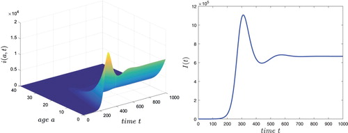
7. Numerical simulation

In this section, we give some numerical simulations to illustrate the theoretical results in Sections 2 and 3. The backward Euler and linearized finite difference method will be used to discretize the ODEs and PDE in system (3(3) $\begin{array}{rl}\dot{S}(t)& =A-{\mu }_{S}S(t)-S(t){\int }_0^{\mathrm{\infty }}\beta (a)i(a,t)\mathrm{d}a,\\ {\displaystyle \frac{\mathrm{\partial }e(\theta ,t)}{\mathrm{\partial }t}+{\displaystyle \frac{\mathrm{\partial }e(\theta ,t)}{\mathrm{\partial }\theta }}}& =-(\mu (\theta )+\epsilon (\theta ))e(\theta ,t),\theta >0,\\ {\displaystyle \frac{\mathrm{\partial }i(a,t)}{\mathrm{\partial }t}+{\displaystyle \frac{\mathrm{\partial }i(a,t)}{\mathrm{\partial }a}}}& =-\nu (a)i(a,t),a>0\end{array}$(3) ), and the integral will be numerically calculated using Simpson's rule.

The transmission coefficient of active infectious individuals at age of infection a is chosen as: (88) $\beta (a)=\{\begin{array}{ll}3\times {10}^{-7}{\mathrm{person}}^{-1}{\mathrm{year}}^{-1},& a<1,\\ 1.5\times {10}^{-7}{\mathrm{person}}^{-1}{\mathrm{year}}^{-1},& a\ge 1.\end{array}$(88) The other parameters in system (3(3) $\begin{array}{rl}\dot{S}(t)& =A-{\mu }_{S}S(t)-S(t){\int }_0^{\mathrm{\infty }}\beta (a)i(a,t)\mathrm{d}a,\\ {\displaystyle \frac{\mathrm{\partial }e(\theta ,t)}{\mathrm{\partial }t}+{\displaystyle \frac{\mathrm{\partial }e(\theta ,t)}{\mathrm{\partial }\theta }}}& =-(\mu (\theta )+\epsilon (\theta ))e(\theta ,t),\theta >0,\\ {\displaystyle \frac{\mathrm{\partial }i(a,t)}{\mathrm{\partial }t}+{\displaystyle \frac{\mathrm{\partial }i(a,t)}{\mathrm{\partial }a}}}& =-\nu (a)i(a,t),a>0\end{array}$(3) ) are chosen as follows: (89) $\begin{array}{rl}& A=2\times {10}^5\mathrm{people}\mathrm{yea}{\mathrm{r}}^{-1},{\mu }_S=1/70\mathrm{yea}{\mathrm{r}}^{-1},\nu (a)=0.1612\mathrm{yea}{\mathrm{r}}^{-1},\\ & p=0.05,\mu (\theta )=1/70\mathrm{yea}{\mathrm{r}}^{-1},\epsilon (\theta )=0.00256\mathrm{yea}{\mathrm{r}}^{-1}.\end{array}$(89) The initial condition is chosen as $S(0)=1.4\times {10}^7,e_0(\theta )={\mathrm{e}}^{-\theta },i_0(a)={\mathrm{e}}^{-a}$.

By calculation, we obtain the basic reproduction number ${\mathcal{R}}_0=\mathrm{2.4827.}$ It is easy to see that in addition to the infection-free steady state $E_1(1.4\times {10}^7,0,0)$, system (3(3) $\begin{array}{rl}\dot{S}(t)& =A-{\mu }_{S}S(t)-S(t){\int }_0^{\mathrm{\infty }}\beta (a)i(a,t)\mathrm{d}a,\\ {\displaystyle \frac{\mathrm{\partial }e(\theta ,t)}{\mathrm{\partial }t}+{\displaystyle \frac{\mathrm{\partial }e(\theta ,t)}{\mathrm{\partial }\theta }}}& =-(\mu (\theta )+\epsilon (\theta ))e(\theta ,t),\theta >0,\\ {\displaystyle \frac{\mathrm{\partial }i(a,t)}{\mathrm{\partial }t}+{\displaystyle \frac{\mathrm{\partial }i(a,t)}{\mathrm{\partial }a}}}& =-\nu (a)i(a,t),a>0\end{array}$(3) ) has an endemic steady state $E^{\ast }(5.6389\times {10}^6,2.0014\times {10}^4{\varphi }_2(a),1.1347\times {10}^5{\varphi }_1(\theta ))$ which is locally asymptotically stable. Numerical simulation illustrates this fact (see Figure 1) (we plotted the $i(a,t)$ component only, denote $I(t)={\int }_0^{75}i(a,t)\mathrm{d}a$).

Figure 1. The temporal solution found by numerical integration of system (3(3) $\begin{array}{rl}\dot{S}(t)& =A-{\mu }_{S}S(t)-S(t){\int }_0^{\mathrm{\infty }}\beta (a)i(a,t)\mathrm{d}a,\\ {\displaystyle \frac{\mathrm{\partial }e(\theta ,t)}{\mathrm{\partial }t}+{\displaystyle \frac{\mathrm{\partial }e(\theta ,t)}{\mathrm{\partial }\theta }}}& =-(\mu (\theta )+\epsilon (\theta ))e(\theta ,t),\theta >0,\\ {\displaystyle \frac{\mathrm{\partial }i(a,t)}{\mathrm{\partial }t}+{\displaystyle \frac{\mathrm{\partial }i(a,t)}{\mathrm{\partial }a}}}& =-\nu (a)i(a,t),a>0\end{array}$(3) ) with the boundary conditions (4(4) $\begin{array}{rl}e(0,t)& =(1-p)S(t){\int }_0^{\mathrm{\infty }}\beta (a)i(a,t)\mathrm{d}a,\\ i(0,t)& =pS(t){\int }_0^{\mathrm{\infty }}\beta (a)i(a,t)\mathrm{d}a+{\int }_0^{\mathrm{\infty }}\epsilon (\theta )e(\theta ,t)\mathrm{d}\theta ,\end{array}$(4) ) and the initial condition $S(0)=1.4\times {10}^7,e_0(\theta )={\mathrm{e}}^{-\theta },i_0(a)={\mathrm{e}}^{-a}$, and the parameters given in (88(88) $\beta (a)=\{\begin{array}{ll}3\times {10}^{-7}{\mathrm{person}}^{-1}{\mathrm{year}}^{-1},& a<1,\\ 1.5\times {10}^{-7}{\mathrm{person}}^{-1}{\mathrm{year}}^{-1},& a\ge 1.\end{array}$(88) ) and (89(89) $\begin{array}{rl}& A=2\times {10}^5\mathrm{people}\mathrm{yea}{\mathrm{r}}^{-1},{\mu }_S=1/70\mathrm{yea}{\mathrm{r}}^{-1},\nu (a)=0.1612\mathrm{yea}{\mathrm{r}}^{-1},\\ & p=0.05,\mu (\theta )=1/70\mathrm{yea}{\mathrm{r}}^{-1},\epsilon (\theta )=0.00256\mathrm{yea}{\mathrm{r}}^{-1}.\end{array}$(89) ).

8. Discussion

In this work, a mathematical model describing tuberculosis transmission with fast and slow progression and age-dependent latency and infection was investigated. By calculations, the basic reproduction number was obtained. It has been shown that the global dynamics of system (3(3) $\begin{array}{rl}\dot{S}(t)& =A-{\mu }_{S}S(t)-S(t){\int }_0^{\mathrm{\infty }}\beta (a)i(a,t)\mathrm{d}a,\\ {\displaystyle \frac{\mathrm{\partial }e(\theta ,t)}{\mathrm{\partial }t}+{\displaystyle \frac{\mathrm{\partial }e(\theta ,t)}{\mathrm{\partial }\theta }}}& =-(\mu (\theta )+\epsilon (\theta ))e(\theta ,t),\theta >0,\\ {\displaystyle \frac{\mathrm{\partial }i(a,t)}{\mathrm{\partial }t}+{\displaystyle \frac{\mathrm{\partial }i(a,t)}{\mathrm{\partial }a}}}& =-\nu (a)i(a,t),a>0\end{array}$(3) ) with boundary conditions (4(4) $\begin{array}{rl}e(0,t)& =(1-p)S(t){\int }_0^{\mathrm{\infty }}\beta (a)i(a,t)\mathrm{d}a,\\ i(0,t)& =pS(t){\int }_0^{\mathrm{\infty }}\beta (a)i(a,t)\mathrm{d}a+{\int }_0^{\mathrm{\infty }}\epsilon (\theta )e(\theta ,t)\mathrm{d}\theta ,\end{array}$(4) ) and initial condition (5(5) $X_0:=(S(0),e(\cdot ,0),i(\cdot ,0))=(S^0,e_0(\cdot ),i_0(\cdot ))\in \mathcal{X},$(5) ) is completely determined by the basic reproduction number. By constructing suitable Lyapunov functionals and using LaSalle's invariance principle, it has been verified that if the basic reproduction number is less than unity, the disease-free steady state is globally asymptotically stable and the disease dies out; and if the basic reproduction number is greater than unity, the endemic steady state is globally asymptotically stable and the disease persists. The global stability of the endemic steady state rules out any possibility for the existence of Hopf bifurcations and sustained oscillations in system (3(3) $\begin{array}{rl}\dot{S}(t)& =A-{\mu }_{S}S(t)-S(t){\int }_0^{\mathrm{\infty }}\beta (a)i(a,t)\mathrm{d}a,\\ {\displaystyle \frac{\mathrm{\partial }e(\theta ,t)}{\mathrm{\partial }t}+{\displaystyle \frac{\mathrm{\partial }e(\theta ,t)}{\mathrm{\partial }\theta }}}& =-(\mu (\theta )+\epsilon (\theta ))e(\theta ,t),\theta >0,\\ {\displaystyle \frac{\mathrm{\partial }i(a,t)}{\mathrm{\partial }t}+{\displaystyle \frac{\mathrm{\partial }i(a,t)}{\mathrm{\partial }a}}}& =-\nu (a)i(a,t),a>0\end{array}$(3) ) with boundary conditions (4(4) $\begin{array}{rl}e(0,t)& =(1-p)S(t){\int }_0^{\mathrm{\infty }}\beta (a)i(a,t)\mathrm{d}a,\\ i(0,t)& =pS(t){\int }_0^{\mathrm{\infty }}\beta (a)i(a,t)\mathrm{d}a+{\int }_0^{\mathrm{\infty }}\epsilon (\theta )e(\theta ,t)\mathrm{d}\theta ,\end{array}$(4) ). A similar dynamic behavior has been observed in [36,37].

In the following, we present some special cases of system (3(3) $\begin{array}{rl}\dot{S}(t)& =A-{\mu }_{S}S(t)-S(t){\int }_0^{\mathrm{\infty }}\beta (a)i(a,t)\mathrm{d}a,\\ {\displaystyle \frac{\mathrm{\partial }e(\theta ,t)}{\mathrm{\partial }t}+{\displaystyle \frac{\mathrm{\partial }e(\theta ,t)}{\mathrm{\partial }\theta }}}& =-(\mu (\theta )+\epsilon (\theta ))e(\theta ,t),\theta >0,\\ {\displaystyle \frac{\mathrm{\partial }i(a,t)}{\mathrm{\partial }t}+{\displaystyle \frac{\mathrm{\partial }i(a,t)}{\mathrm{\partial }a}}}& =-\nu (a)i(a,t),a>0\end{array}$(3) ) with the boundary conditions (4(4) $\begin{array}{rl}e(0,t)& =(1-p)S(t){\int }_0^{\mathrm{\infty }}\beta (a)i(a,t)\mathrm{d}a,\\ i(0,t)& =pS(t){\int }_0^{\mathrm{\infty }}\beta (a)i(a,t)\mathrm{d}a+{\int }_0^{\mathrm{\infty }}\epsilon (\theta )e(\theta ,t)\mathrm{d}\theta ,\end{array}$(4) ).

Example 8.1

When p = 0, then the boundary conditions (4(4) $\begin{array}{rl}e(0,t)& =(1-p)S(t){\int }_0^{\mathrm{\infty }}\beta (a)i(a,t)\mathrm{d}a,\\ i(0,t)& =pS(t){\int }_0^{\mathrm{\infty }}\beta (a)i(a,t)\mathrm{d}a+{\int }_0^{\mathrm{\infty }}\epsilon (\theta )e(\theta ,t)\mathrm{d}\theta ,\end{array}$(4) ) reduce to the following: (90) $\begin{array}{rl}e(0,t)& =S(t){\int }_0^{\mathrm{\infty }}\beta (a)i(a,t)\mathrm{d}a,\\ i(0,t)& ={\int }_0^{\mathrm{\infty }}\epsilon (\theta )e(\theta ,t)\mathrm{d}\theta .\end{array}$(90) The global dynamics of system (3(3) $\begin{array}{rl}\dot{S}(t)& =A-{\mu }_{S}S(t)-S(t){\int }_0^{\mathrm{\infty }}\beta (a)i(a,t)\mathrm{d}a,\\ {\displaystyle \frac{\mathrm{\partial }e(\theta ,t)}{\mathrm{\partial }t}+{\displaystyle \frac{\mathrm{\partial }e(\theta ,t)}{\mathrm{\partial }\theta }}}& =-(\mu (\theta )+\epsilon (\theta ))e(\theta ,t),\theta >0,\\ {\displaystyle \frac{\mathrm{\partial }i(a,t)}{\mathrm{\partial }t}+{\displaystyle \frac{\mathrm{\partial }i(a,t)}{\mathrm{\partial }a}}}& =-\nu (a)i(a,t),a>0\end{array}$(3) ) with the boundary conditions (90(90) $\begin{array}{rl}e(0,t)& =S(t){\int }_0^{\mathrm{\infty }}\beta (a)i(a,t)\mathrm{d}a,\\ i(0,t)& ={\int }_0^{\mathrm{\infty }}\epsilon (\theta )e(\theta ,t)\mathrm{d}\theta .\end{array}$(90) ) has been established in [28] by constructing suitable Lyapunov functionals and using LaSalle's invariance principle. It has been shown from Theorems 7.1 and 9.5 in [28] that system (3(3) $\begin{array}{rl}\dot{S}(t)& =A-{\mu }_{S}S(t)-S(t){\int }_0^{\mathrm{\infty }}\beta (a)i(a,t)\mathrm{d}a,\\ {\displaystyle \frac{\mathrm{\partial }e(\theta ,t)}{\mathrm{\partial }t}+{\displaystyle \frac{\mathrm{\partial }e(\theta ,t)}{\mathrm{\partial }\theta }}}& =-(\mu (\theta )+\epsilon (\theta ))e(\theta ,t),\theta >0,\\ {\displaystyle \frac{\mathrm{\partial }i(a,t)}{\mathrm{\partial }t}+{\displaystyle \frac{\mathrm{\partial }i(a,t)}{\mathrm{\partial }a}}}& =-\nu (a)i(a,t),a>0\end{array}$(3) ) with the boundary conditions (90(90) $\begin{array}{rl}e(0,t)& =S(t){\int }_0^{\mathrm{\infty }}\beta (a)i(a,t)\mathrm{d}a,\\ i(0,t)& ={\int }_0^{\mathrm{\infty }}\epsilon (\theta )e(\theta ,t)\mathrm{d}\theta .\end{array}$(90) ) admits the same global dynamics as system (3(3) $\begin{array}{rl}\dot{S}(t)& =A-{\mu }_{S}S(t)-S(t){\int }_0^{\mathrm{\infty }}\beta (a)i(a,t)\mathrm{d}a,\\ {\displaystyle \frac{\mathrm{\partial }e(\theta ,t)}{\mathrm{\partial }t}+{\displaystyle \frac{\mathrm{\partial }e(\theta ,t)}{\mathrm{\partial }\theta }}}& =-(\mu (\theta )+\epsilon (\theta ))e(\theta ,t),\theta >0,\\ {\displaystyle \frac{\mathrm{\partial }i(a,t)}{\mathrm{\partial }t}+{\displaystyle \frac{\mathrm{\partial }i(a,t)}{\mathrm{\partial }a}}}& =-\nu (a)i(a,t),a>0\end{array}$(3) ) with the boundary conditions (4(4) $\begin{array}{rl}e(0,t)& =(1-p)S(t){\int }_0^{\mathrm{\infty }}\beta (a)i(a,t)\mathrm{d}a,\\ i(0,t)& =pS(t){\int }_0^{\mathrm{\infty }}\beta (a)i(a,t)\mathrm{d}a+{\int }_0^{\mathrm{\infty }}\epsilon (\theta )e(\theta ,t)\mathrm{d}\theta ,\end{array}$(4) ).

Example 8.2

In system (3(3) $\begin{array}{rl}\dot{S}(t)& =A-{\mu }_{S}S(t)-S(t){\int }_0^{\mathrm{\infty }}\beta (a)i(a,t)\mathrm{d}a,\\ {\displaystyle \frac{\mathrm{\partial }e(\theta ,t)}{\mathrm{\partial }t}+{\displaystyle \frac{\mathrm{\partial }e(\theta ,t)}{\mathrm{\partial }\theta }}}& =-(\mu (\theta )+\epsilon (\theta ))e(\theta ,t),\theta >0,\\ {\displaystyle \frac{\mathrm{\partial }i(a,t)}{\mathrm{\partial }t}+{\displaystyle \frac{\mathrm{\partial }i(a,t)}{\mathrm{\partial }a}}}& =-\nu (a)i(a,t),a>0\end{array}$(3) ), we suppose (91) ${\mu }_S=\mu ,\beta (a)\equiv \beta ,\mu (\theta )\equiv \mu ,\epsilon (\theta )\equiv \nu ,\nu (a)\equiv \mu +{\mu }_T,$(91) where $\beta ,\mu ,\nu$ and ${\mu }_T$ are positive constants. Let $L(t)={\int }_0^{\mathrm{\infty }}e(\theta ,t)\mathrm{d}\theta ,I(t)={\int }_0^{\mathrm{\infty }}i(a,t)\mathrm{d}a$.

Solving the second equation of system (3(3) $\begin{array}{rl}\dot{S}(t)& =A-{\mu }_{S}S(t)-S(t){\int }_0^{\mathrm{\infty }}\beta (a)i(a,t)\mathrm{d}a,\\ {\displaystyle \frac{\mathrm{\partial }e(\theta ,t)}{\mathrm{\partial }t}+{\displaystyle \frac{\mathrm{\partial }e(\theta ,t)}{\mathrm{\partial }\theta }}}& =-(\mu (\theta )+\epsilon (\theta ))e(\theta ,t),\theta >0,\\ {\displaystyle \frac{\mathrm{\partial }i(a,t)}{\mathrm{\partial }t}+{\displaystyle \frac{\mathrm{\partial }i(a,t)}{\mathrm{\partial }a}}}& =-\nu (a)i(a,t),a>0\end{array}$(3) ) with the boundary condition (4(4) $\begin{array}{rl}e(0,t)& =(1-p)S(t){\int }_0^{\mathrm{\infty }}\beta (a)i(a,t)\mathrm{d}a,\\ i(0,t)& =pS(t){\int }_0^{\mathrm{\infty }}\beta (a)i(a,t)\mathrm{d}a+{\int }_0^{\mathrm{\infty }}\epsilon (\theta )e(\theta ,t)\mathrm{d}\theta ,\end{array}$(4) ) and the initial condition (5(5) $X_0:=(S(0),e(\cdot ,0),i(\cdot ,0))=(S^0,e_0(\cdot ),i_0(\cdot ))\in \mathcal{X},$(5) ) yields (92) $e(\theta ,t)=\{\begin{array}{ll}e(0,t-\theta ){\mathrm{e}}^{-{\int }_0^{\theta }(\mu +\nu )\mathrm{d}s},& 0\le \theta \le t,\\ e_0(\theta -t){\mathrm{e}}^{-{\int }_{\theta -t}^{\theta }(\mu +\nu )\mathrm{d}s},& 0\le t\le \theta .\end{array}$(92) When t is sufficiently large (being greater than all possible infection ages), we have (93) $e(\theta ,t)=e(0,t-\theta ){\mathrm{e}}^{-{\int }_0^{\theta }(\mu +\nu )\mathrm{d}s}=e(0,t-\theta ){\mathrm{e}}^{-(\mu +\nu )\theta }.$(93) It therefore follows from (3(3) $\begin{array}{rl}\dot{S}(t)& =A-{\mu }_{S}S(t)-S(t){\int }_0^{\mathrm{\infty }}\beta (a)i(a,t)\mathrm{d}a,\\ {\displaystyle \frac{\mathrm{\partial }e(\theta ,t)}{\mathrm{\partial }t}+{\displaystyle \frac{\mathrm{\partial }e(\theta ,t)}{\mathrm{\partial }\theta }}}& =-(\mu (\theta )+\epsilon (\theta ))e(\theta ,t),\theta >0,\\ {\displaystyle \frac{\mathrm{\partial }i(a,t)}{\mathrm{\partial }t}+{\displaystyle \frac{\mathrm{\partial }i(a,t)}{\mathrm{\partial }a}}}& =-\nu (a)i(a,t),a>0\end{array}$(3) ), (90(90) $\begin{array}{rl}e(0,t)& =S(t){\int }_0^{\mathrm{\infty }}\beta (a)i(a,t)\mathrm{d}a,\\ i(0,t)& ={\int }_0^{\mathrm{\infty }}\epsilon (\theta )e(\theta ,t)\mathrm{d}\theta .\end{array}$(90) ) and (93(93) $e(\theta ,t)=e(0,t-\theta ){\mathrm{e}}^{-{\int }_0^{\theta }(\mu +\nu )\mathrm{d}s}=e(0,t-\theta ){\mathrm{e}}^{-(\mu +\nu )\theta }.$(93) ) that (94) $\begin{array}{rl}{\displaystyle \frac{\mathrm{d}}{\mathrm{d}t}L(t)}& ={\int }_0^{\mathrm{\infty }}{\displaystyle \frac{e(\theta ,t)}{\mathrm{\partial }t}\mathrm{d}\theta }\\ & =-{\int }_0^{\mathrm{\infty }}{\displaystyle \frac{\mathrm{\partial }e(\theta ,t)}{\mathrm{\partial }\theta }\mathrm{d}\theta -{\int }_0^{\mathrm{\infty }}(\mu +\nu )e(\theta ,t)\mathrm{d}\theta }\\ & =-e(\theta ,t){|}_0^{\mathrm{\infty }}-(\mu +\nu ){\int }_0^{\mathrm{\infty }}e(\theta ,t)\mathrm{d}\theta \\ & =(1-p)S(t){\int }_0^{\mathrm{\infty }}\beta i(a,t)\mathrm{d}a-(\mu +\nu ){\int }_0^{\mathrm{\infty }}e(\theta ,t)\mathrm{d}\theta \\ & =(1-p)\beta S(t)I(t)-(\mu +\nu )L(t).\end{array}$(94) Similarly, we have (95) ${\displaystyle \frac{\mathrm{d}}{\mathrm{d}t}I(t)=p\beta S(t)I(t)+\nu L(t)-(\mu +{\mu }_T)I(t).}$(95) Hence, system (3(3) $\begin{array}{rl}\dot{S}(t)& =A-{\mu }_{S}S(t)-S(t){\int }_0^{\mathrm{\infty }}\beta (a)i(a,t)\mathrm{d}a,\\ {\displaystyle \frac{\mathrm{\partial }e(\theta ,t)}{\mathrm{\partial }t}+{\displaystyle \frac{\mathrm{\partial }e(\theta ,t)}{\mathrm{\partial }\theta }}}& =-(\mu (\theta )+\epsilon (\theta ))e(\theta ,t),\theta >0,\\ {\displaystyle \frac{\mathrm{\partial }i(a,t)}{\mathrm{\partial }t}+{\displaystyle \frac{\mathrm{\partial }i(a,t)}{\mathrm{\partial }a}}}& =-\nu (a)i(a,t),a>0\end{array}$(3) ) with the boundary conditions (4(4) $\begin{array}{rl}e(0,t)& =(1-p)S(t){\int }_0^{\mathrm{\infty }}\beta (a)i(a,t)\mathrm{d}a,\\ i(0,t)& =pS(t){\int }_0^{\mathrm{\infty }}\beta (a)i(a,t)\mathrm{d}a+{\int }_0^{\mathrm{\infty }}\epsilon (\theta )e(\theta ,t)\mathrm{d}\theta ,\end{array}$(4) ) and the initial condition (5(5) $X_0:=(S(0),e(\cdot ,0),i(\cdot ,0))=(S^0,e_0(\cdot ),i_0(\cdot ))\in \mathcal{X},$(5) ) reduces to system (1(1) $\begin{array}{rl}\dot{S}(t)& =A-\mu S(t)-\beta S(t)I(t),\\ \dot{L}(t)& =(1-p)\beta S(t)I(t)-\nu L(t)-\mu L(t),\\ \dot{I}(t)& =p\beta S(t)I(t)+\nu L(t)-(\mu +{\mu }_T)I(t).\end{array}$(1) ). The global dynamics of system (1(1) $\begin{array}{rl}\dot{S}(t)& =A-\mu S(t)-\beta S(t)I(t),\\ \dot{L}(t)& =(1-p)\beta S(t)I(t)-\nu L(t)-\mu L(t),\\ \dot{I}(t)& =p\beta S(t)I(t)+\nu L(t)-(\mu +{\mu }_T)I(t).\end{array}$(1) ) was investigated in [22] by means of Lyapunov functions and LaSalle's invariance principle. It has been verified in [22] that system (1(1) $\begin{array}{rl}\dot{S}(t)& =A-\mu S(t)-\beta S(t)I(t),\\ \dot{L}(t)& =(1-p)\beta S(t)I(t)-\nu L(t)-\mu L(t),\\ \dot{I}(t)& =p\beta S(t)I(t)+\nu L(t)-(\mu +{\mu }_T)I(t).\end{array}$(1) ) has the same global dynamics as system (3(3) $\begin{array}{rl}\dot{S}(t)& =A-{\mu }_{S}S(t)-S(t){\int }_0^{\mathrm{\infty }}\beta (a)i(a,t)\mathrm{d}a,\\ {\displaystyle \frac{\mathrm{\partial }e(\theta ,t)}{\mathrm{\partial }t}+{\displaystyle \frac{\mathrm{\partial }e(\theta ,t)}{\mathrm{\partial }\theta }}}& =-(\mu (\theta )+\epsilon (\theta ))e(\theta ,t),\theta >0,\\ {\displaystyle \frac{\mathrm{\partial }i(a,t)}{\mathrm{\partial }t}+{\displaystyle \frac{\mathrm{\partial }i(a,t)}{\mathrm{\partial }a}}}& =-\nu (a)i(a,t),a>0\end{array}$(3) ) with the boundary conditions (4(4) $\begin{array}{rl}e(0,t)& =(1-p)S(t){\int }_0^{\mathrm{\infty }}\beta (a)i(a,t)\mathrm{d}a,\\ i(0,t)& =pS(t){\int }_0^{\mathrm{\infty }}\beta (a)i(a,t)\mathrm{d}a+{\int }_0^{\mathrm{\infty }}\epsilon (\theta )e(\theta ,t)\mathrm{d}\theta ,\end{array}$(4) ) and the initial condition (5(5) $X_0:=(S(0),e(\cdot ,0),i(\cdot ,0))=(S^0,e_0(\cdot ),i_0(\cdot ))\in \mathcal{X},$(5) ).

From the expression of the basic reproduction number ${\mathcal{R}}_0$ of system (3(3) $\begin{array}{rl}\dot{S}(t)& =A-{\mu }_{S}S(t)-S(t){\int }_0^{\mathrm{\infty }}\beta (a)i(a,t)\mathrm{d}a,\\ {\displaystyle \frac{\mathrm{\partial }e(\theta ,t)}{\mathrm{\partial }t}+{\displaystyle \frac{\mathrm{\partial }e(\theta ,t)}{\mathrm{\partial }\theta }}}& =-(\mu (\theta )+\epsilon (\theta ))e(\theta ,t),\theta >0,\\ {\displaystyle \frac{\mathrm{\partial }i(a,t)}{\mathrm{\partial }t}+{\displaystyle \frac{\mathrm{\partial }i(a,t)}{\mathrm{\partial }a}}}& =-\nu (a)i(a,t),a>0\end{array}$(3) ), we see that the introduction of the age structure has significant influence on the value of the basic reproduction number of tuberculosis transmission. In fact, a direct calculation shows that with the assumption (91(91) ${\mu }_S=\mu ,\beta (a)\equiv \beta ,\mu (\theta )\equiv \mu ,\epsilon (\theta )\equiv \nu ,\nu (a)\equiv \mu +{\mu }_T,$(91) ), ${\mathcal{R}}_0$ reduces to ${\mathcal{R}}_0$, the basic reproduction number of epidemiological model (1(1) $\begin{array}{rl}\dot{S}(t)& =A-\mu S(t)-\beta S(t)I(t),\\ \dot{L}(t)& =(1-p)\beta S(t)I(t)-\nu L(t)-\mu L(t),\\ \dot{I}(t)& =p\beta S(t)I(t)+\nu L(t)-(\mu +{\mu }_T)I(t).\end{array}$(1) ). We note that it is assumed in system (1(1) $\begin{array}{rl}\dot{S}(t)& =A-\mu S(t)-\beta S(t)I(t),\\ \dot{L}(t)& =(1-p)\beta S(t)I(t)-\nu L(t)-\mu L(t),\\ \dot{I}(t)& =p\beta S(t)I(t)+\nu L(t)-(\mu +{\mu }_T)I(t).\end{array}$(1) ) that all parameters are positive constants and all individuals within a compartment behave identically, regardless of how much time they have spent in the compartment. For instance, infectious individuals are assumed to be equally infectious during their periodic infectivity and the waiting times in each compartment are assumed to be exponentially distributed. In system (3(3) $\begin{array}{rl}\dot{S}(t)& =A-{\mu }_{S}S(t)-S(t){\int }_0^{\mathrm{\infty }}\beta (a)i(a,t)\mathrm{d}a,\\ {\displaystyle \frac{\mathrm{\partial }e(\theta ,t)}{\mathrm{\partial }t}+{\displaystyle \frac{\mathrm{\partial }e(\theta ,t)}{\mathrm{\partial }\theta }}}& =-(\mu (\theta )+\epsilon (\theta ))e(\theta ,t),\theta >0,\\ {\displaystyle \frac{\mathrm{\partial }i(a,t)}{\mathrm{\partial }t}+{\displaystyle \frac{\mathrm{\partial }i(a,t)}{\mathrm{\partial }a}}}& =-\nu (a)i(a,t),a>0\end{array}$(3) ), we included the duration that an individual has spent in the latently infected compartment and in the active infectious compartment as continuous variables. Hence, ${\mathcal{R}}_0$ can be used to describe the number of new infections generated by a single newly infectious individual during the full infectious period more accurately than ${\mathcal{R}}_0$. This indicates that although ODE models without age structure are usually easier to use than PDE models with age structure, it could lead to the over-valuation or underestimation of the basic reproduction number of tuberculosis transmission.

By choosing appropriate kernel functions, system (3(3) $\begin{array}{rl}\dot{S}(t)& =A-{\mu }_{S}S(t)-S(t){\int }_0^{\mathrm{\infty }}\beta (a)i(a,t)\mathrm{d}a,\\ {\displaystyle \frac{\mathrm{\partial }e(\theta ,t)}{\mathrm{\partial }t}+{\displaystyle \frac{\mathrm{\partial }e(\theta ,t)}{\mathrm{\partial }\theta }}}& =-(\mu (\theta )+\epsilon (\theta ))e(\theta ,t),\theta >0,\\ {\displaystyle \frac{\mathrm{\partial }i(a,t)}{\mathrm{\partial }t}+{\displaystyle \frac{\mathrm{\partial }i(a,t)}{\mathrm{\partial }a}}}& =-\nu (a)i(a,t),a>0\end{array}$(3) ) also contains epidemiological models with time delay, and the global stability results in this work provide the global dynamics for these delayed epidemic models.

Acknowledgments

The authors wish to thank the reviewers and the Editor for their careful reading, valuable comments and suggestions that greatly improved the presentation of this work.

Disclosure statement

No potential conflict of interest was reported by the authors.

Correction Statement

This article was originally published with errors, which have now been corrected in the online version. Please see Correction (http://doi.org/10.1080/17513758.2020.1761137)

Additional information

Funding

This work was supported by the National Natural Science Foundation of China [grant numbers 11871316, 11801340, 61573016, 11371368] and the Natural Science Foundation of Shanxi Province [grant numbers 201801D121006, 201801D221007].

References

- J.P. Aparicio and C. Castillo-Chavez, Mathematical modelling of tuberculosis epidemics, Math. Biosci. Eng. 6 (2009), pp. 209–237. doi: 10.3934/mbe.2009.6.209
- J.P. Aparicio, A.F. Capurro, and C. Castillo-Chavez, Transmission and dynamics of tuberculosis on generalized households, J. Theor. Biol. 206 (2000), pp. 327–341. doi: 10.1006/jtbi.2000.2129
- J.P. Aparicio, A.F. Capurro, and C. Castillo-Chavez, Markers of disease evolution: The case of tuberculosis, J. Theor. Biol. 215 (2002), pp. 227–237. doi: 10.1006/jtbi.2001.2489
- G. Bjune, Tuberculosis in the 21st century: An emerging pandemic? Norsk Epidemiologi 15 (2005), pp. 133–139.
- S.M Blower and T. Chou, Modeling the emergence of the ‘hot zones’ tuberculosis and the amplification dynamics of drug resistance, Nat. Med. 10 (2004), pp. 1111–1116. doi: 10.1038/nm1102
- S.M. Blower, A.R. McLean, T.C. Porco, P.M. Small, P.C. Hopwell, M.A. Sanchez, and A.R. Moss, The intrinsic transmission dynamics of tuberculosis epidemics, Nat. Med. 1 (1995), pp. 815–821. doi: 10.1038/nm0895-815
- S.M. Blower, P.M. Small, and P.C. Hopewell, Control strategies for tuberculosis epidemics: New models for old problems, Science 273 (1996), pp. 497–500. doi: 10.1126/science.273.5274.497
- F. Brauer, Z. Shuai, and P. van den Driessche, Dynamics of an age-of-infection cholera model, Math. Biosci. Eng. 10 (2013), pp. 1335–1349. doi: 10.3934/mbe.2013.10.1335
- T.F. Brewer and S.J. Heymann, To control and beyond: Moving towards eliminating the global tuberculosis threat, J. Epidemiol. Community Health 58 (2004), pp. 822–825. doi: 10.1136/jech.2003.008664
- C. Castillo-Chavez and Z. Feng, To treat or not to treat: The case of tuberculosis, J. Math. Biol. 35 (1997), pp. 629–656. doi: 10.1007/s002850050069
- C. Castillo-Chavez and Z. Feng, Global stability of an age-structure model for TB and its applications to optimal vaccination strategies, Math. Biosci. 151 (1998), pp. 135–154. doi: 10.1016/S0025-5564(98)10016-0
- C. Castillo-Chavez and B. Song, Dynamical models of tuberculosis and their applications, Math. Biosci. Eng. 1(2) (2004), pp. 361–404. doi: 10.3934/mbe.2004.1.361
- Y. Chen, J. Yang, and F. Zhang, The global stability of an SIRS model with infection age, Math. Biosci. Eng. 11 (2014), pp. 449–469. doi: 10.3934/mbe.2014.11.449
- E. Corbett, C. Watt, N. Walker, D. Maher, B. Williams, M. Raviglione, and C. Dye, The growing burden of tuberculosis: Global trends and interactions with the HIV epidemic, Arch. Intern. Med. 163 (2003), pp. 1009–1021. doi: 10.1001/archinte.163.9.1009
- X. Duan, S. Yuan, Z. Qiu, and J. Ma, Global stability of an SVEIR epidemic model with ages of vaccination and latency, Comput. Math. Appl. 68 (2014), pp. 288–308. doi: 10.1016/j.camwa.2014.06.002
- X. Duan, S. Yuan, and X. Li, Global stability of an SVIR model with age of vaccination, Appl. Math. Comput. 226 (2014), pp. 528–540.
- A. Ducrot and P. Magal, Travelling wave solutions for an infection-age structured epidemic model with external supplies, Nonlineaity 24 (2011), pp. 2891–2911. doi: 10.1088/0951-7715/24/10/012
- C. Dye and B.G. Williams, Criteria for the control of drug-resistant tuberculosis, Proc. Natl. Acad. Sci. USA 97 (2000), pp. 8180–8185. doi: 10.1073/pnas.140102797
- Z. Feng, C. Castillo-Chavez, and A.F. Capurro, A model for tuberculosis with exogenous reinfection, Theor. Popul. Biol. 57 (2000), pp. 235–247. doi: 10.1006/tpbi.2000.1451
- Z. Feng, W. Huang, and C. Castillo-Chavez, On the role of variable latent periods in mathematical models for tuberculosis, J. Dyn. Differ. Equ. 13 (2001), pp. 425–452. doi: 10.1023/A:1016688209771
- Z. Feng, M. Iannelli, and F.A. Milner, A two-strain tuberculosis model with age of infection, SIAM J. Appl. Math. 62 (2002), pp. 1634–1656. doi: 10.1137/S003613990038205X
- H. Guo, Global dynamics of a mathematical model of tuberculosis, Can. Appl. Math. Quart. 13(4) (2005), pp. 313–323.
- J.K. Hale and P. Waltman, Persistence in infinite dimensional systems, SIAM J. Math. Anal. 20 (1989), pp. 388–395. doi: 10.1137/0520025
- M. Iannelli, Mathematical Theory of Age-Structured Population Dynamics, Applied Mathematics Monographs 7, comitato nazionale per le scienze matematiche, Consiglio Nazionale delle Ricerche (C.N.R), Giardini, Pisa, 1995.
- S. Lawn, R. Wood, and R. Wilkinson, Changing concepts of ‘latent tuberculosis infection’ in patients living with HIV infection, Clin. Dev. Immunol. 2011 (2011), p. 980594. doi: 10.1155/2011/980594
- P. Magal, Compact attractors for time periodic age-structured population models, Electron. J. Differ. Equ. 2001(65) (2001), pp. 1–35.
- P. Magal, C.C. McCluskey, and G.F. Webb, Lyapunov functional and global asymptotic stability for an infection-age model, Appl. Anal. 89 (2010), pp. 1109–1140. doi: 10.1080/00036810903208122
- C.C. McCluskey, Global stability for an SEI epidemiological model with continuous age-structure in the exposed and infectious classes, Math. Biosci. Eng. 9 (2012), pp. 819–841. doi: 10.3934/mbe.2012.9.819
- B. Miller, Preventive therapy for tuberculosis, Med. Clin. North Am. 77 (1993), pp. 1263–1275. doi: 10.1016/S0025-7125(16)30192-4
- P. Rodriguesa, M.G.M. Gomes, and C. Rebelo, Drug resistance in tuberculosis: A reinfection model, Theor. Popul. Biol. 71 (2007), pp. 196–212. doi: 10.1016/j.tpb.2006.10.004
- H.L. Smith and H.R. Thieme, Dynamical Systems and Population Persistence, American Mathematical Society, Providence, 2011.
- C. Ted and M. Megan, Modeling epidemics of multidrug resistant M. tuberculosis of heterogeneous fitness, Nat. Med. 10 (2004), pp. 1117–1121. doi: 10.1038/nm1110
- P. van den Driessche and J. Watmough, Reproduction numbers and sub-threshold endemic equilibria for compartmental models of disease transmission, Math. Biosci. 180 (2002), pp. 29–48. doi: 10.1016/S0025-5564(02)00108-6
- W.H.O. Report, Global Tuberculosis Control: Epidemiology, Strategy, Financing, World Health Organization, Geneva, 2009.
- G. Webb, Theory of Nonlinear Age-Dependent Population Dynamics, Marcel Dekker, New York, 1985.
- R. Xu, Global dynamics of an epidemiological model with age of infection and disease relapse, J. Biol. Dyn, 12(1) (2018), pp. 118–145. doi: 10.1080/17513758.2017.1408860
- R. Xu, X. Tian & S. Zhang, An age-structured within host HIV-1 infection model with virus-to-cell and cell-to-cell transmissions, J. Biol. Dyn., 12(1) (2018), pp. 89–117. doi: 10.1080/17513758.2017.1404646
- J. Yang, X. Li, and M. Martcheva, Global stability of a DS-DI epidemic model with age of infection, J. Math. Anal. Appl. 385 (2012), pp. 655–671. doi: 10.1016/j.jmaa.2011.06.087
- J. Yang, Z. Qiu, and X. Li, Global stability of an age-structured cholera model, Math. Biosci. Eng. 11 (2014), pp. 641–665. doi: 10.3934/mbe.2014.11.641