
 ?Mathematical formulae have been encoded as MathML and are displayed in this HTML version using MathJax in order to improve their display. Uncheck the box to turn MathJax off. This feature requires Javascript. Click on a formula to zoom.
Abstract
In this paper, Melnikov analysis of chaos in a simple SIR model with periodically or stochastically modulated nonlinear incidence rate and the effect of periodic and bounded noise on the chaotic motion of SIR model possessing homoclinic orbits are detailed investigated. Based on homoclinic bifurcation, necessary conditions for possible chaotic motion as well as sufficient condition are derived by the random Melnikov theorem, and to establish the threshold of bounded noise amplitude for the onset of chaos.
1. Introduction
A classical SIR model is considered and the model postulates a constant population which is divided into three classes: susceptible individuals (S), infected individuals (I) and recovered individuals (R). The assumption of constant population size is therefore mathematically expressed by S+I+R=1. Vital dynamics are taken into account by considering a natural mortality rate per capita and a number μ of births per time unit. Let
denote the rate of transmission per infective so that a number
of individuals leave the susceptible compartment to pass into the infective one. We assume that
is periodic or stochastic, with period
and an infected individual may recover at the rate
.
Dynamics are therefore described by the following system
(1)
(1) which has been extensively studied [Citation22,Citation23,Citation27]. More complicated forms of the incidence function have been studied. Liu et al. studied the codimension-1 bifurcation for SEIRS and SIRS models with the incidence rate
in [Citation20,Citation21]. Derrick and van den Driessche [Citation8] studied saddle-node bifurcation, Hopf bifurcation and Bogdanov–Takens bifurcation of SIRS or SIR models with the incidence rate of
. Ruan and Wang [Citation30] studied saddle-node bifurcation, Hopf bifurcation, Bogdanov–Takens bifurcation and the existence of none, one and two limit cycles of an SIRS model with an incidence rate of
, which was also proposed by Liu et al. [Citation21]. Van den Driessche and Watmough [Citation33,Citation34] studied an incidence rate of the form
, where
and
. When
this incidence rate is the bilinear incidence rate
[Citation6]. In [Citation34], they studied an SIS model with this incidence rate for
and k=2, showing the backward bifurcation, local stability and global stability of equilibria. In [Citation33], they further introduced the same incidence rate in an SIRS model. Alexander and Moghadas [Citation1] analysed an SIV model with a generalized nonlinear incidence rate
and showed the existence of bistability and various Hopf bifurcation, especially for the incidence rate
with
and
. Jin et al. [Citation16] give a detailed theoretical analysis of the SIRS model with the incidence rate
, clearly show the effect of this nonlinear incidence rate on the transmission dynamics of epidemics, not only theoretically obtained backward bifurcation, Hopf bifurcation and Bogdanov–Takens bifurcation for this SIRS model, but also shown bistable steady states and explicit conditions for asymptotic stability of equilibria, even for globally asymptotic stability, and especially found stability switches for one of the endemic equilibria.
In (Equation1(1)
(1) ),
(called the transmission rate) is either constant or a periodic modulation about a constant value, for example:
(2)
(2) Greenman et al. [Citation14] understand the structure of possible modes of ecological and epidemiological system oscillation with the simplest case of seasonality supposed that
, in particular, the conditions under which they appear and disappear that the multiplicity, typically created by a hierarchy of subcritical subharmonics can lead to high amplification of the forcing signal and complex switching under chaos and stochastic externalities. Yi et al. [Citation37] studied the periodic, chaotic and hyperchaotic dynamical behavior of an SEIR epidemic system governed by differential and algebraic equations with seasonal forcing in transmission form
. Nakata and Kuniya [Citation26] studied a class of periodic SEIR epidemic models and it is shown that the global dynamics is determined by the basic reproduction number
. Best [Citation4] used bifurcation analysis to investigate the effects of seasonal forcing in the form
on the already complex epidemiological dynamics of the SPI model. More recent models, motivated by biological realism, rather than mathematical simplicity, have taken the contact rate to be governed by the school terms
(3)
(3) where
is a periodic function which is
during school terms and
during school holidays [Citation5,Citation11]. However, throughout this paper, an alternative and more natural, form will be used
(4)
(4) Although these two forms are equivalent after rescaling parameters, the second form is far more convenient as we do not have to place an upper bound on
. Augeraud-Veron and Sari [Citation3] consider a seasonally forced SIR epidemic model where periodicity occurs in the contact rate of the form
where
and
. Olinky et al. [Citation28] provide new insights into the dynamics of recurrent diseases and specific predictions about individual outbreaks using the seasonally forced SIR epidemic model, the contact rate is same as [Citation3].
It is in particular well-known that when is sufficiently large in (Equation2
(2)
(2) ), it is possible to obtain strong numerical evidence of chaotic motion in these examples [Citation2,Citation17,Citation29]. As
was varied, a period-doubling route to chaos was observed [Citation13], this generated much excitement and prompted many researchers to look for chaos in epidemiological time series [Citation12,Citation31,Citation32]. Chaotic behaviour has been observed numerically in many numerical simulations of forced SIR models, and in slightly more complicated models which take into account the time delay between being infected and becoming infective (SEIR models). The arguments, for example in the context of measles, tend to concentrate on the relatively large values of necessary to observe chaotic trajectories. Glendinning and Perry [Citation13] have utilized a periodically forced nonlinear incidence rate to prove that there are SIR models with chaotic trajectories. The choice of the incidence function used is
with the transmission rate
(5)
(5) where ε is a small positive parameter and Ω is the frequency of harmonic excitation. Diallo and Kon [Citation9] establishes mathematically the existence of chaotic motion of the SIR models by Melnikov's method through a series of coordinate transformations to bring the equations into amenable to Melnikov analysis. The choice of the incidence function used is
with the transmission rate
(6)
(6) where
are same as (Equation5
(5)
(5) ), and
is a periodic function. Diallo et al. [Citation10] studied the well-known SIR model of epidemic dynamics with an almost periodic incidence rate in the form
with the transmission rate
(7)
(7) where
are same as above, and
is a (possibly not periodic) almost periodic function. It maked the use of similar techniques utilized in recent work to establish the existence of chaotic motions.
In this paper, we will consider the incidence function , which may vary periodically and stochastically with time and the transmission rate is
(8)
(8) where
and
are order one constants such that
(9)
(9) is also of order one. If p=2,
in (Equation7
(7)
(7) ) can be transformed into 16 in (Equation8
(8)
(8) ). Nevertheless, there is an almost periodically in (Equation7
(7)
(7) ) and periodically and stochastically in (Equation8
(8)
(8) ) forced nonlinear incidence rate. The latter is more complex which be unaware of any work for proving mathematically that can be chaotic.
We will also assume that
(10)
(10) Thus we are dealing with a disease for which the timescales for infection, recovery and reproduction are all of the same order of magnitude and such that the transmission rate varies very slowly (assuming that μ is bounded as ε tends to zero).
is belong to stochastic excitation and called bounded noise to be described that is a harmonic function with constant amplitude and random frequency and phase. The mathematical expression for the bounded noise is
(11)
(11) where
and σ are positive constant.
is harmonic excitation, and
and
represent the amplitude or level of the harmonic and stochastic (bounded noise) excitation, respectively.
is the frequency of harmonic and
is average frequency of bounded noise. σ is the strength of the noise.
is a standard Wiener process, Γ is a random variable uniformly distributed in
representing a random phase angle.
is a broad-band stationary bounded stochastic process in a wide sense with zero mean which is non-Gaussian distribution [Citation19]. Its covariance function is
(12)
(12) The variance of the bounded noise is
which implies that the bounded noise has finite power. Its spectral density is
(13)
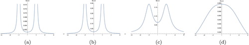
(13) The spectral density of bounded noise for several sets of parameters is shown in Figure . The position of peak of the spectral density depends on
, and the bandwidth of the bounded noise depends mainly on σ. It has density function
For
,
is a bounded stochastic process, it is still a continuous process which satisfies the conditions which can deduce the Melnikov function [Citation35,Citation36]. Modifying the value of
and σ one can obtain different band width.When
will be narrow band process and if
will approach a white noise which has constant power. Choosing proper values for
and
may represent the turbulent flow in the wind and the motion of seismic floor. So it is reasonable to add the bounded noise as a stochastic excitation. It can be shown that the sample functions of the noise are continuous and bounded which are required in the derivation of the random Melnikov process [Citation18,Citation24,Citation25].
Figure 1. The spectral density of bounded noise for . (a)
. (b)
. (c)
and (d)
.
In this paper, our aim is to explore the effect of periodic and bounded noise excitation on the chaotic motion of system (Equation1(1)
(1) ) by using the stochastic Melnikov method. The paper is organized as follows. In Section 2, the random Melnikov process for Hamiltonian system subject to light damping and external or parametric perturbation of bounded noise is derived. We describe the scaling of the SIR variables which will allow us to use Melnikov's method in Section 3. The crucial step here is to identify a doubly degenerate stationary point close to which the equations can be seen as a perturbation of a nearly Hamiltonian system, and then to determine the appropriate scaling of the variables which allow Melnikov's method to be applied. In Section 4, this method is used to prove the existence of chaotic solutions in the SIR model with periodic and random transmission rates. Conclusions are made in Section 5.
2. Random Melnikov process
Consider a single degree-of-freedom Hamiltonian system subject to light damping and weakly external and (or) parametric excitations of bounded noise. The equation of motion of the system is of the form
(14)
(14) where x and y are generalized displacement and momentum, respectively;
is Hamiltonian with continuous first-order derivatives; ε is a small positive parameter;
denotes the coefficient of quasi-linear damping;
denotes the amplitude of excitation.
is an external excitation of bounded noise if f is a constant. Otherwise, it is a parametric excitation. It is assumed that the Hamiltonian system associated with Equation (Equation14
(14)
(14) ) possesses a hyperbolic fixed point connected to itself by homoclinic orbits
.
A bounded noise with spectral density (Equation13(13)
(13) ) can be approximated by a sum of many harmonic functions with different frequency and random phases. As in [Citation25], the random Melnikov process for system (Equation14
(14)
(14) ) is
(15)
(15) where
is the component of Melnikov process due to damping and
is that due to bounded noise excitation. Note that
and
in the integrand of Equation (Equation15
(15)
(15) ) are taken as
and
of homoclinic orbit. Obviously, the mean of random Melnikov process is
(16)
(16) where
denotes the expectation operator. For positive damping, Equation (Equation16
(16)
(16) ) always yields a negative value, which implies that system (Equation14
(14)
(14) ) cannot be chaotic in mean sense. The mean-square values of the two components of random Melnikov process (Equation15
(15)
(15) ) are
(17)
(17)
(18)
(18) To calculate
,
in Equation (Equation15
(15)
(15) ) is rewritten as a convolution integral
(19)
(19) where
can be regarded as the impulse response function of a time-invariant linear system while
as an input to the system. Thus, the variance of the system can be obtained in the frequency domain as follows:
(20)
(20) where
is the frequency response function of the system, which is the Fourier transformation of the impulse response function
.
Random Melnikov process (Equation15(15)
(15) ) has a simple zero in the the mean-square sense when
(21)
(21) which yield the threshold amplitude of bounded noise excitation for the onset of chaos in the system (Equation14
(14)
(14) ).
3. Scaling the equations
Since S=1−I−R the basic SIR model, (Equation1(1)
(1) ) can be written as
(22)
(22) Define a new timescale
with respect to which the equations are independent of μ, so
(23)
(23) where
and
.
We need to change coordinates in such a way that the system is able to use the Melnikov method. We will make a succession of changes of coordinates to bring the equation into a standard form, based around the fact that near certain degenerate stationary points it is, typically, possible to write the equations as perturbations of a Hamiltonian system. Link in [Citation9], our first aim is to make some changes of coordinates in order to adapt the system (Equation23(23)
(23) ) to the Melnikov analysis.
We shall work with (Equation23(23)
(23) ), and for the remainder of this section we shall drop the primes to avoid making the equations look worse than they are. Begin by defining a new variable
, so (Equation23
(23)
(23) ) becomes
(24)
(24) where the dots denote differentiation with respect to the rescaled time. After a little manipulation, substituting (Equation23
(23)
(23) ) into the second equation of (Equation24
(24)
(24) ) and using
, so (Equation24
(24)
(24) ) becomes
(25)
(25) Stationary points of (Equation25
(25)
(25) ) clear have z=0 and either R=0 which corresponds to the disease-free equilibrium, or z=0 and R satisfies
(26)
(26) This quadratic (Equation26
(26)
(26) ) has two real roots if
that is
We obtain by simplifying
So the system (Equation25
(25)
(25) ) has a saddle-node bifurcation if
At this value, the equilibrium, supporting an endemic level of the disease, is
The Jacobian matrix of the system (Equation25
(25)
(25) ) at z=0 is
where
The determinant of this matrix
equals to 0 at
, but if, in addition, the trace
also equals to 0, then we have a more degenerate situation, Known as a Takens–Bogdanov point and near this point it should be possible to write the equations in nearly Hamiltonian form as required if the Melnikov method is to be applied [Citation15]. The trace of the Jacobian matrix equals to 0 at the saddle-node point (where
) if
(27)
(27) For these values of parameters, the degenerate equilibrium is
Note that a curve of Hopf bifurcation also terminates at this point. This curve is given by
To perturb about this degenerate equilibrium point we define new variables and parameters by
where
and b are to be thought of as small (they will be chosen in accordance with (Equation8
(8)
(8) )–(Equation10
(10)
(10) ) in Section 1, but for the moment it is instructive to think of them as arbitrary small numbers, so that the scaling of Section 1 are demystified. Substituting into (Equation25
(25)
(25) ) and ignoring cubic order and higher we find
(28)
(28) We introduce the small parameter ε by setting
(29)
(29) In accordance with (Equation8
(8)
(8) ), so
Defining new coordinates and time by
gives
and so, setting
, we obtain
(30)
(30) On further rescaling brings this equation into a standard form [37]: let
then Equations (Equation30
(30)
(30) ) become
(31)
(31) where
, where is a strictly positive order one constant by assumption (Equation9
(9)
(9) ). In the following we suppose that c>0.
Equation (Equation31(31)
(31) ) with
and
is a standard normal form for the Takens–Bogdanov bifurcation, and an extensive analysis can be found in Chow et al. [Citation7]. The dynamics is boring if
so assume that
and
. Then there are two stationary points:
,
is a saddle and
if
then
if
if
The bifurcation at is a standard (subcritical) hopf bifurcation, and the bifurcation which destroys the periodic orbit at
is a homoclinic (global) bifurcation.
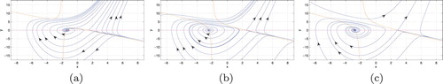
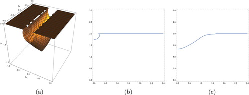
The phase portraits are shown in Figure (a–c) for . (a):
, (b):
, (c):
, respectively. In Figure (a),
is a saddle, and
is an unstable focus. In Figure (b),
is a saddle, and
is a stable focus and is surrounded by an unstable periodic orbit. In Figure (c),
is a saddle, and
is a stable focus, and there are no periodic orbits encircling it.
Figure 2. Phase portraits of the system (Equation31(31)
(31) ) for
.(a)
. (b)
and (c)
4. Chaos in the SIR model with periodically or stochastically modulated nonlinear incidence rate
We can apply Melnikov method to the SIR model in the form (Equation31(31)
(31) ) for sufficiently small ε. If
, Equation (Equation31
(31)
(31) ) is considered as an unperturbed system and can be written as
(32)
(32) where dots now denote differentiation with respect to the rescaled time τ and c>0. Equation (Equation32
(32)
(32) ) is a Hamiltonian system with Hamiltonian function
(33)
(33) and so solution lie on curves of constant H. The function
is called the potential function. The Jacobian matrix is
. The characteristic polynomial is
. Equation (Equation32
(32)
(32) ) is well- known in the literature [Citation15]. It has two stationary points:
, which is a saddle and
, which is a centre. The centre is surrounded by a continuous family of periodic orbits,
and these are bounded by a homoclinic orbit
such that
The explicit form of the homoclinic solution [Citation15] is
(34)
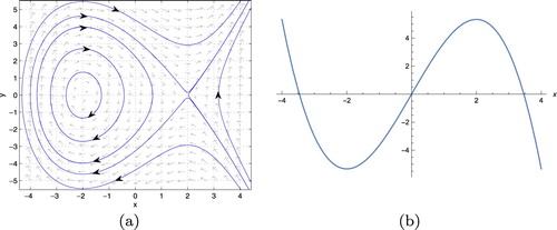
(34) The phase portrait and potential diagram are shown in Figure (a,b) for
, respectively. In Figure (a),
is a centre and
is a saddle, which is connected itself by homoclinic orbits
.
Figure 3. Phase portrait and potential of the system (Equation32(32)
(32) ) for
. (a) Phase portrait. (b) Potential.
In the following, three cases are considered and is the cross-section time of the Pioncar
map and
can be interpreted as the initial time of the forcing term.
Case 1: Now we can find the Melnikov function of system (Equation31(31)
(31) ) without stochastic excitation
as follows:
(35)
(35) If the Melnikov function has simple zero point, the stable manifolds and the unstable manifolds intersect transversally, chaos in the sense of Smale horseshoe transform will occur. So let
, the criterion for the existence of a zero of this Melnikov function is easy to obtain from
.
, where
(36)
(36) and the following theorem can be obtained.
Theorem 4.1
If , the stable and unstable manifolds of the fixed point in the Poincar
map intersect transversely and there is chaos in the model, whilst if
, there is no intersection between the stable and unstable manifolds. At
there is a tangential intersection between the stable and unstable manifolds.
If , then
, it takes a particularly simple form:
, where
The homoclinic bifurcation curve for Smale chaos in the
plane for
and
in Figure (a,b), respectively. In the parameter region below the bifurcation curve, no transverse intersection of stable and unstable manifolds of saddle occurs and above the bifurcation curve, the transverse intersections of stable and unstable manifolds of the saddle occur. Just above the homoclinic bifurcation curve onset of cross-well chaos is expected.
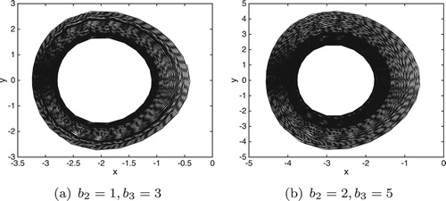
The phase portraits of the system (Equation31(31)
(31) ) for
and
are plotted in Figure (a,b). By simple calculating with (Equation36
(36)
(36) ),
and 4.27242, respectively. We can see that the motion of system (Equation31
(31)
(31) ) are chaotic from Figure .
Figure 4. The homoclinic bifurcation curve for Smale chaos in the plane. (a)
and (b)
.
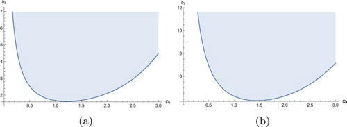
Figure 5. Phase portrait with and initial value:
. (a)
and (b)
.
Case 2: Now we can find the Melnikov function of system (Equation31(31)
(31) ) with two periodic excitation
as follows:
(37)
(37) where
The criterion for the existence of a zero of this Melnikov function is obtained from
and
. Therefore we obtain criteria for the existence of chaos in two periodic forced system (Equation31
(31)
(31) ) if
(38)
(38)
Theorem 4.2
Suppose the condition (Equation38(38)
(38) ) is satisfied, then a homoclinic bifurcation occurs, then the system (Equation31
(31)
(31) ) may exhibits chaotic motion.
The upper bound of possible chaotic domain due to the homoclinic bifurcation for the cases without noise perturbation of system (Equation31(31)
(31) ) is obtained by equating the expressions in (Equation38
(38)
(38) ) and portrayed in Figure (a). It depict the domains of possible occurrence of chaotic motion in
space. The upper bounds are also presented in Figure (b,c) with
and
for the case without noise perturbation in
and
plane, respectively. From Figure one can see that the presence of two periodic excitation enlarges the threshold amplitude and reduces the possible chaotic domain in small parameter space.
Figure 6. Upper bound for possible chaotic domain due to homoclinic bifurcation with
. (a) Upper surface in
space. (b) Upper bound in
plane with
and (c) Upper bound in
plane with
.
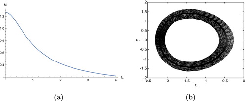
Let
then the condition (Equation38
(38)
(38) ) is written as
(38′)
(38′) The bifurcation curve (Equation38′
(38′)
(38′) ) for the homoclinic orbit
covering the range
are plotted in Figure (a). From it we can see that when the value of
increases, the value of M decreases. It is easy to know that if the parameter values are chosen from the region M<1, the system (Equation31
(31)
(31) ) can exist chaotic dynamics. For example, for the fixed parameter values
and
, when
, there is M<1. The chaotic trajectory at
are shown in Figure (b).
Figure 7. (a) Bifurcation curve for the homoclinic orbits
. Here
and
; (b) Phase portrait for (Equation31
(31)
(31) ) with
and initial value:
.
Case 3: Now we can find the Melnikov function of system (Equation31(31)
(31) ) just with stochastic excitation (
).
The random Melnikov function for this problem is therefore (from (Equation31(31)
(31) ))
(39)
(39) where
(40)
(40) and
(41)
(41) The first two integral in (Equation39
(39)
(39) ) represent the mean of the Melnikov process due to damping force, and the last integral denotes the random portion of the Melnikov process due to bounded noise
. We can analyse the simple zero point of
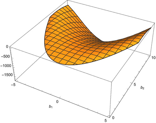
in probability or statistics sense. Consider the mean of random process
is zero, one can get
. If it gives a non-zero constant, that is to say in mean sense chaos never occurs in system (Equation31
(31)
(31) ). If it equals to zero, in the mean-value sense the condition for the occurrence of chaotic motion in the sense of Smale horseshoe transform is
. The surface
in
plane is shown in Figure .
Figure 8. The surface in plane for
.
Now, let us consider if random Melnikov process (Equation39(39)
(39) ) has simple zeros on mean-square sense. In this case, the impulse response function is
(42)
(42) and the associated frequency response function of the system is
(43)
(43) i.e. the Fourier transformation of the impulse response function
. Note that
has zero mean. We can also consider whether the mean value of
and
may be equal. Since that
(44)
(44)
(45)
(45)
is the spectral density of
. Random Melnikov process has simple zeros in mean-square sense if
(46)
(46) The variance of
as the output of the system can be expressed as follows.
(47)
(47)
Theorem 4.3
The criterion for possible chaotic motion based on Melnikov process is performed in mean-square representation , i.e.
(48)
(48)
The integral in (Equation48(48)
(48) ) can be calculated by numerical method. Numerical computation has been made for the following parameter values:
. The mean-square criterion in (Equation46
(46)
(46) ) yields the threshold of bounded noise amplitude for the onset of chaos in the system (Equation31
(31)
(31) ) by numerical computation, which is shown in Figure (a,b).
Figure 9. The threshold amplitude of bounded noise excitation for the onset of chaos in system (Equation31
(31)
(31) ) with
. (a)
.
![Figure 9. The threshold amplitude b4 of bounded noise excitation for the onset of chaos in system (Equation31(31) dxdτ=y,dydτ=−c2+x2+ϵ(b1y+xy−4b3sin(Ω1τ)−4b4ξ(τ))+o(ϵ2),(31) ) with b3=0,b1=2,b2=3/2,Ω2=2. (a) σ∈[0,3];(b)σ∈[0,1].](/cms/asset/e2476ddf-70d3-45e7-84b5-247f93f6ddb8/tjbd_a_1718222_f0009_oc.jpg)
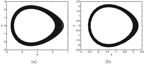
The phase portraits of the system (Equation31(31)
(31) ) for
and
are shown in from Figure (a,b). We can see the chaos orbits.
Figure 10. Phase portraits of the system (Equation31(31)
(31) ) with
and
. (a)
with initial value:
. (b)
with initial value:
.
5. Conclusion
In this paper, the effect of periodic and bounded noise on the chaotic motion of SIR model possessing homoclinic orbits is detailed investigated. Based on homoclinic bifurcation, necessary conditions for possible chaotic motion as well as sufficient condition are derived by the random Melnikov theorem, and to establish the threshold of bounded noise amplitude for onset of chaos. The results indicate that the presence of larger noise enhances the threshold amplitude and reduces the possible chaotic domain in parameter space. Numerical calculation of the phase portraits of the original system also validates that the threshold amplitude
for onset of chaos will move upwards as the noise intensity increases for larger noise intensity. The results reveal chaotic attractor is diffused by bounded noise, and the larger the noise intensity results in the more diffused attractor.
However, for chaos in model with periodically and stochastically modulated nonlinear incidence rate, further investigation is needed to clarify the inconsistency between the two kinds of thresholds given by the random Melnikov method with the associated mean-square criterion and by the numerical simulation of the Pioncar maps. In addition, the criterion for possible chaotic motion in system (Equation31
(31)
(31) ) with periodic and stochastic excitation is performed analytically and further numerical validation is needed.
Acknowledgments
The author is very thankful to the referee for careful reading of the paper and valuable suggestions and useful comments that improved the presentation of the paper.
Disclosure statement
No potential conflict of interest was reported by the author.
ORCID
Yanxiang Shi http://orcid.org/0000-0002-6134-200X
Additional information
Funding
References
- M.E. Alexander and S.M. Moghadas, Periodicity in an epidemic model with a generalized non-linear incidence, Math. Biosci. 189 (2004), pp. 75–96. doi: 10.1016/j.mbs.2004.01.003
- J.L. Aron and I.B. Schwartz, Seasonality and period-doubling bifurcations in an epidemic model, J. Theor. Biol. 110 (1984), pp. 665–679. doi: 10.1016/S0022-5193(84)80150-2
- E. Augeraud-Veron and N. Sari, Seasonal dynamics in an SIR epidemic system, J. Math. Biol. 68 (2014), pp. 701–725. doi: 10.1007/s00285-013-0645-y
- A. Best, The Effects of seasonal forcing on invertebrate-disease interactions with immune priming, Bull. Math. Biol. 75 (2013), pp. 2241–2256. doi: 10.1007/s11538-013-9889-3
- B.M. Bolker, Chaos and complexity in measles models: A comparative numerical study, IMA J. Math. Appl. Med. Biol. 10 (1993), pp. 83–95. doi: 10.1093/imammb/10.2.83
- F. Brauer and P. van den Driessche, Models for translation of disease with immigration of infectives, Math. Biosci. 171 (2001), pp. 143–154. doi: 10.1016/S0025-5564(01)00057-8
- S.N. Chow, C. Li, and D. Wang, Normal Forms and Bifurcation of Planar Vector Fields, Cambridge, Cambridge University Press, 1994.
- W.R. Derrick and P. van den Driessche, Homoclinic orbits in a disease transmission model with nonlinear incidence and nonconstant population, Discrete Cont. Dyn. Sys. Ser. B 3 (2003), pp. 299–309.
- O. Diallo and Y. Kon, Melnikov analysis of chaos in a general epidemiological model, Nonlinear Anal. Real World Appl. 8 (2007), pp. 20–26. doi: 10.1016/j.nonrwa.2005.03.032
- O. Diallo, Y. Kon, and A. Maiga, Melnikov analysis of chaos in an epidemiological model with almost periodic incidence rates, Appl. Math. Sci. 2 (2008), pp. 1377–1386.
- D.J.D. Earn, P. Rohani, B.M. Bolker, and B.T. Grenfell, A simple model for complex dynamical transitions in epidemics, Science 287 (2000), pp. 667–670. doi: 10.1126/science.287.5453.667
- S. Ellner and P. Turchin, Chaos in a noisy world: New methods and evidence from time series analysis, Amer. Natur. 145 (1995), pp. 343–375. doi: 10.1086/285744
- P. Glendinning and L.P. Perry, Melnikov analysis of chaos in a simple epidemiological model, J. Math. Biol. 35 (1997), pp. 359–373. doi: 10.1007/s002850050056
- J. Greenmail, M. Kamo, and M. Boots, External forcing of ecological and epidemiological systems: A resonance approach, Physica D 190 (2004), pp. 136–151. doi: 10.1016/j.physd.2003.08.008
- J. Guckenheimer and P. Holmes, Nonlinear Oscillations, Dynamical Systems, and Bifurcations of Vector Fields, New York, Springer, 1983.
- Y. Jin, W.D. Wang, and S.W. Xiao, An SIRS model with a nonlinear incidence rate, Chaos Soliton Fract. 34 (2007), pp. 1482–1497. doi: 10.1016/j.chaos.2006.04.022
- Yu. A. Kuznetsov and C. Piccardi, Bifurcation analysis of periodic SEIR and SIR epidemic models, J. Math. Biol. 32 (1994), pp. 109–121. doi: 10.1007/BF00163027
- J.R. Li, W Xu, X.L. Yang, and Z.K. Sun, Chaotic motion of Van der Pol Mathieu Duffing system under bounded noise parametric excitation, J. Sound Vib. 309 (2008), pp. 330–337. doi: 10.1016/j.jsv.2007.05.027
- Y.K. Lin and G.Q. Cai, Probabilistic Structural Dynamics: Advanced Theory and Applications, McGraw-Hill, NewYork, 1995.
- W.M. Liu, H.W. Hethcote, and S.A. Levin, Dynamical behavior of epidemiological models with nonlinear incidence rates, J. Math. Biol. 25 (1987), pp. 359–380. doi: 10.1007/BF00277162
- W.M. Liu, S.A. Levin, and Y. Iwasa, Influence of nonlinear incidence rates upon the behavior of SIRS epidemiological models, J. Math. Biol. 23 (1986), pp. 187–204. doi: 10.1007/BF00276956
- X.Z. Liu and P. Stechlinski, Pulse and constant control schemes for epidemic models with seasonality, Nonlinear Anal. Real World Appl. 12 (2011), pp. 931–946. doi: 10.1016/j.nonrwa.2010.08.017
- X.Z. Liu and P. Stechlinski, Infectious disease models with time-varying parameters and general nonlinear incidence rate, Appl. Math. Model. 36 (2012), pp. 1974–1994. doi: 10.1016/j.apm.2011.08.019
- Z.H. Liu and W.Q. Zhu, Homoclinic bifurcation and chaos in simple pendulum under bounded noise excitation, Chaos Soliton Fract. 20 (2004), pp. 593–607. doi: 10.1016/j.chaos.2003.08.010
- W.Y. Liu, W.Q. Zhu, and Z.L. Huang, Eect of bounded noise on chaotic motion of duffing oscillator under parametric excitation, Chaos Soliton Fract. 12 (2001), pp. 527–537. doi: 10.1016/S0960-0779(00)00002-3
- Y. Nakata and T. Kuniya, Global dynamics of a class of SEIRS epidemic models in a periodic environment, J. Math. Anal. Appl. 363 (2010), pp. 230–237. doi: 10.1016/j.jmaa.2009.08.027
- S.M. O'Regan, T.C. Kelly, A. Korobeinikov, M.J.A. O'Callaghan, A.V. Pokrovskii, and D. Rachinskii, Chaos in a seasonally perturbed SIR model: Avian influenza in a seabird colony as a paradigm, J. Math. Biol. 67 (2013), pp. 293–327. doi: 10.1007/s00285-012-0550-9
- R. Olinky, A. Huppert, and L. Stone, Seasonal dynamics and thresholds governing recurrent epidemics, J. Math. Biol. 56 (2008), pp. 827–839. doi: 10.1007/s00285-007-0140-4
- L.F. Olsen and W.M. Shaffer, Chaos versus noisy periodicity: Alternative hypotheses for childhood epidemics, Science 249 (1990), pp. 499–504. doi: 10.1126/science.2382131
- S. Ruan and W. Wang, Dynamical behavior of an epidemic model with a nonlinear incidence rate, J. Differ. Equ. 188 (2003), pp. 135–163. doi: 10.1016/S0022-0396(02)00089-X
- W.M. Schaffer and M. Kot, Nearly one-dimensional dynamics in an epidemic, J. Theor. Biol. 112 (1985), pp. 403–427. doi: 10.1016/S0022-5193(85)80294-0
- G. Sugihara, B.T. Grenfell, and R.M. May, Distinguishing error from chaos in ecological time series, Philos. Trans. Roy. Soc. Lond. Ser. B 330 (1990), pp. 235–251. doi: 10.1098/rstb.1990.0195
- P. van den Driessche and J. Watmough, Epidemic solutions and endemic catastrophes, Fields Inst. Commun. 36 (2003), pp. 247–257.
- P. van den Driessche and J. Watmough, A simple SIS epidemic model with a backward bifurcation, J. Math. Biol. 40 (2004), pp. 525–540. doi: 10.1007/s002850000032
- S. Wiggins, Global Bifurcations and Chaos: Analytical Methods, Springer-Verlag, New York, 1988.
- S. Wiggins, Introduction to Applied Nonlinear Dynamical Systems and Chaos, Springer-Verlag, New York, 1990.
- N. Yi, Q.L. Zhang, K. Mao, D.M. Yang, and Q. Li, Analysis and control of an SEIR epidemic system with nonlinear transmission rate, Math. Comput. Model. 50 (2009), pp. 1498–1513. doi: 10.1016/j.mcm.2009.07.014