Impulsive releases of sterile mosquitoes and interactive dynamics with time delay

Abstract

To investigate the impact of periodic and impulsive releases of sterile mosquitoes on the interactive dynamics between wild and sterile mosquitoes, we adapt the new idea where only those sexually active sterile mosquitoes are included in the modelling process and formulate new models with time delay. We consider different release strategies and compare their model dynamics. Under certain conditions, we derive corresponding model formulations and prove the existence of periodic solutions for some of those models. We provide numerical examples to demonstrate the dynamical complexity of the models and propose further studies.

Keywords:

• Sterile mosquitoes
• periodic and impulsive releases
• periodic solutions
• Filippov-type equations

AMS Subject Classifications:

• 34K09
• 34K13
• 34K20
• 92D25
• 92D30
• 92D40

1. Introduction

To prevent and control mosquito-borne diseases, biological measures have been developed and utilized in certain regions.These include the genetic approaches [8,16,24,26], the sterile insect technique (SIT) [28], and the Wolbachia driven mosquito control technique [4,27,29]. They have played an important role in disease control, and have shown promising and effective. To study the impact and effectiveness of these biological control methods, a good number of mathematical models have been formulated and analyzed. Modeling of transgenesis or paratransgenesis has helped us to gain insight into better strategies in genetically engineering mosquitoes [17,18,20,23]. Models for the study of the suppression effects on the control of mosquitoes by releasing Wolbachia-infected mosquitoes have been formulated [11–13,15,33–36]. To investigate the impacts of utilizing the sterile insect technique (SIT) on mosquito control, models have also been formulated and analyzed [1–3,5,6,14,17–19,31,32], in which several strategies of releases of sterile mosquitoes are proposed, including constant releases, proportional releases, fractional releases, and periodic and impulsive releases. In those studies, the interactive dynamical models are two-dimensional systems where the released sterile mosquitoes have their own dynamical equation.

Different from the existing modelling studies, the author in a recent work [30] proposed a new idea for mosquito population suppression modelling. Note that the fundamental and only role that the released sterile mosquitoes play in the interactive dynamics is to mate with wild mosquitoes such that the mated wild mosquitoes either do not reproduce or their produced eggs will not hatch.

Moreover, the lifespan of male mosquitoes is relatively short, usually less than 10 days. While the mating, one of the critical behaviours that characterize the mosquito life strategy, is the least understood and most understudied [9,25], it is well known that males can mate several times and their sexual lifespan is even much shorter than their ages. During such a short period of time when the sterile mosquitoes are sexually active, it is then reasonable to neglect their death. The author of [30] thus only considers and includes those sexually active mosquitoes in the models and ignores the death of those sterile mosquitoes. With such assumptions, instead of using a variable to present the number of the sterile mosquitoes with an independent dynamical equation, this number of sterile mosquitoes is assumed to be a function given in advance. This seems more realistic and biologically more meaningful in the mathematical modelling of vector-borne diseases, and it is creative and innovative, which seems to be the first in such a direction.

We, in this paper, adapt such an idea in [30] and focus on further developing models with time delay for the interactive wild and sterile mosquitoes where the releases of sterile mosquitoes are periodic and impulsive. We describe our baseline model in Section 2. We then consider different release strategies in which the time to release sterile mosquitoes is either before or after the previously released sterile mosquitoes becoming sexual inactive. We determine the expressions of $g\left(t\right)$ corresponding to different cases in Section 3. Numerical examples are given to demonstrate the dynamical features of the model and to compare the impacts of the different release strategies. Under further assumptions, more detailed descriptions of the release functions are presented which are piecewise step functions. We then derive detailed dynamical equations with time delay based on those step functions and prove the existence of periodic solutions under certain conditions in Section 4. Brief discussions of our findings and model features are given in Section 5.

2. The baseline model

To study the interactive dynamics of wild and sterile mosquitoes, there exist models in the literature which are based on ordinary differential equations including the following one in [5]: (1) $\begin{array}{rl}\frac{\mathrm{d}w}{\mathrm{d}t}& =\left(\frac{aw}{w+g}-\left({\mu }_1+{\xi }_1(w+g)\right)\right)w,\\ \frac{\mathrm{d}g}{\mathrm{d}t}& =B-({\mu }_2+{\xi }_2(w+g))g.\end{array}$(1) Here w and g are the numbers of wild and sterile mosquitoes at time t, respectively, a is the total number of offspring per wild mosquito, per unit of time, $w/(w+g)$ is the fraction of mates with wild mosquitoes, ${\mu }_i$ and ${\xi }_i(w+g),i=1,2$, are the density-independent and density-dependent death rates of wild and sterile mosquitoes, respectively, and B is the rate of releases of sterile mosquitoes.

Mosquitoes undergo complete metamorphosis, going through four distinct stages of development during a lifetime [7]. Inclusion of the stage structure and the larvae maturation to adults thus becomes important and more realistic. Models with stage-structure applied to interactive wild and sterile mosquitoes have been formulated and investigated such as those in [22], which are governed by higher dimension systems of differential equations. In the meantime, by using time delay τ for the larvae maturation of wild mosquitoes, delay differential equation models have been formulated and studied as well such as the following system in [6]: (2) $\begin{array}{rl}\frac{\mathrm{d}w\left(t\right)}{\mathrm{d}t}& =\frac{a{e}^{-{\mu }_0\tau }w(t-\tau )}{w(t-\tau )+g(t-\tau )}w(t-\tau )-\left({\mu }_1+{\xi }_1\left(w\right(t)+g(t\left)\right)\right)w\left(t\right),\\ \frac{\mathrm{d}g\left(t\right)}{\mathrm{d}t}& =B(\cdot )-({\mu }_2+{\xi }_2\left(w\right(t)+g(t\left)\right))g\left(t\right),\end{array}$(2) where $e^{-{\mu }_0\tau }$ is the survival rate of lava mosquitoes, and the initial conditions for the model system are (3) $w(t_0+\theta )=\phi \left(\theta \right)>0,g(t_0+\theta )=\psi \left(\theta \right)>0,\theta \in [-\tau ,0],$(3) where $t_0\ge 0$, and $\phi \left(\theta \right)$ and $\psi \left(\theta \right)$ are both positive and continuous in $[-\tau ,0]$.

Adopting the modelling ideas in [30] and assuming that the death and the dynamics of the sterile mosquitoes with respect to the time variable are negligible, the following model for the wild mosquitoes was formulated in [31]: (4) $\frac{\mathrm{d}w\left(t\right)}{\mathrm{d}t}=\frac{a{e}^{-{\mu }_0\tau }{w}^2(t-\tau )}{w(t-\tau )+g(t-\tau )}-\left(\mu +\xi (w\left(t\right)+g\left(t\right))\right)w\left(t\right),$(4) where $g\left(t\right)$ is the number of released sterile mosquitoes which is a nonnegative function of $t\ge 0$ that satisfies $g\left(t\right)\equiv 0$ for t<0.

We note that $g\left(t\right)$ here is no longer a variable whose dynamics are governed by an independent equation, but can be any given nonnegative function.

In the absence of sterile mosquitoes, we let the zero solution of the model equation be unstable. Thus, we assume (5) $a{e}^{-{\mu }_0\tau }-\mu >0.$(5) hereafter in this paper.

For given $t_0\ge 0$, with an initial function $\phi \in C\left(\right[t_0-\tau ,t_0],(0,\mathrm{\infty }\left)\right)$, and a given nonnegative function $g\left(t\right)$ specified separately on $[t_0-\tau ,t_0],w\left(t\right)=w(t,g,t_0,\phi )$ is said to be a solution of (4(4) $\frac{\mathrm{d}w\left(t\right)}{\mathrm{d}t}=\frac{a{e}^{-{\mu }_0\tau }{w}^2(t-\tau )}{w(t-\tau )+g(t-\tau )}-\left(\mu +\xi (w\left(t\right)+g\left(t\right))\right)w\left(t\right),$(4) ) through $(t_0,\phi )$ if $w\in C^1\left(\right[t_0,\mathrm{\infty }),[0,\mathrm{\infty }\left)\right)$ satisfies (4(4) $\frac{\mathrm{d}w\left(t\right)}{\mathrm{d}t}=\frac{a{e}^{-{\mu }_0\tau }{w}^2(t-\tau )}{w(t-\tau )+g(t-\tau )}-\left(\mu +\xi (w\left(t\right)+g\left(t\right))\right)w\left(t\right),$(4) ) on $[t_0,\mathrm{\infty })$ and $w\left(t\right)=\phi \left(t\right)$ for $t\in [t_0-\tau ,t_0]$. It is easy to see that, since $\phi \left(t\right)>0$ for $t_0-\tau \le t\le t_0$, we have $w\left(t\right)>0$ for all $t\ge t_0$. We assume that the release starts at time t = 0. Then $g\left(t\right)=0$ for $t\le 0$ and $g\left(0^{+}\right)$ denotes the number of the released sterile mosquitoes for the first time.

We first give a few definitions below for the convenience of the reader.

Definition 2.1

[30]

A solution $w_0\left(t\right)$ of (4(4) $\frac{\mathrm{d}w\left(t\right)}{\mathrm{d}t}=\frac{a{e}^{-{\mu }_0\tau }{w}^2(t-\tau )}{w(t-\tau )+g(t-\tau )}-\left(\mu +\xi (w\left(t\right)+g\left(t\right))\right)w\left(t\right),$(4) ) is said to be

• Stable if for any $t_0\ge 0$ and $\epsilon >0$, there exists $\delta >0$ such that $\phi \in C\left(\right[t_0-\tau ,t_0],(0,\mathrm{\infty }\left)\right)$ and $|\phi \left(t\right)-w_0\left(t\right)|<\delta$ for $t\in [t_0-\tau ,t_0]$ implies $\left|w\left(t\right)-w_0\left(t\right)\right|=\left|w(t,g,t_0,\phi )-w_0\left(t\right)\right|<\epsilon ,\text{for }t\ge t_0.$If δ is independent of $t_0$, then $w_0\left(t\right)$ is uniformly stable.

• Stable from the right-side (or left-side) if for any $t_0\ge 0$ and $\epsilon >0$, there exists $\delta >0$ such that $\phi \in C\left(\right[t_0-\tau ,t_0],(0,\mathrm{\infty }\left)\right)$ and $0<\phi \left(t\right)-w_0\left(t\right)<\delta$ (or $0>\phi \left(t\right)-w_0\left(t\right)>-\delta$) for $t\in [t_0-\tau ,t_0]$ implies $w\left(t\right)-w_0\left(t\right)=w(t,g,t_0,\phi )-w_0\left(t\right)\in (0,\epsilon )(\text{or}\in (-\epsilon ,0\left)\right),\text{for }t\ge t_0.$

• Semi-stable if it is stable from the right-side (or left-side) but unstable from the left-side (or right-side).

• Globally asymptotically stable if it is uniformly stable, and for any $t_0\ge 0,\phi \in C\left(\right[t_0-\tau ,t_0],(0,\mathrm{\infty }\left)\right)$ $\underset{t\to \mathrm{\infty }}{lim}(w(t,g,t_0,\phi )-w_0\left(t\right))=0.$

We list the general analytic results of the dynamics of (4(4) $\frac{\mathrm{d}w\left(t\right)}{\mathrm{d}t}=\frac{a{e}^{-{\mu }_0\tau }{w}^2(t-\tau )}{w(t-\tau )+g(t-\tau )}-\left(\mu +\xi (w\left(t\right)+g\left(t\right))\right)w\left(t\right),$(4) ) as follows. More details can be found in [31].

Theorem 2.1

Define the threshold value of releases for (4(4) $\frac{\mathrm{d}w\left(t\right)}{\mathrm{d}t}=\frac{a{e}^{-{\mu }_0\tau }{w}^2(t-\tau )}{w(t-\tau )+g(t-\tau )}-\left(\mu +\xi (w\left(t\right)+g\left(t\right))\right)w\left(t\right),$(4) ) by (6) $g^{\ast }=\frac{{\left(a{e}^{-{\mu }_0\tau }-\mu \right)}^2}{4a\xi e^{-{\mu }_0\tau }}.$(6) Assume that there exist two positive constants $g_1<g_2\le g^{\ast }$ such that $g\left(t\right)\in [g_1,g_2]$ for all t>0. Then the trivial equilibrium $E_0$ of (4(4) $\frac{\mathrm{d}w\left(t\right)}{\mathrm{d}t}=\frac{a{e}^{-{\mu }_0\tau }{w}^2(t-\tau )}{w(t-\tau )+g(t-\tau )}-\left(\mu +\xi (w\left(t\right)+g\left(t\right))\right)w\left(t\right),$(4) ) is uniformly asymptotically stable. Moreover, $\underset{t\to \mathrm{\infty }}{lim}w(t,g,t_0,\phi )=0,$ for any $\phi \in C\left(\right[t_0-\tau ,t_0],(0,E\left(g_1\right)\left)\right)$ for $t\in [t_0-\tau ,t_0]$ and $\underset{t\to \mathrm{\infty }}{lim}w(t,g,t_0,\phi )\ne 0$ for any $\phi \left(t\right)>E\left(g_2\right)$ for $t\in [t_0-\tau ,t_0]$. Here $E\left(g_i\right):=-g_i+\frac{a{e}^{-{\mu }_0\tau }-\mu }{2\xi }\left(1-\sqrt{1-\frac{g_i}{g^{\ast }}}\right).$

Theorem 2.2

Assume $\underset{t\in (0,\mathrm{\infty })}{inf}g\left(t\right)>g^{\ast }$. Then the trivial equilibrium $E_0=0$ of (4(4) $\frac{\mathrm{d}w\left(t\right)}{\mathrm{d}t}=\frac{a{e}^{-{\mu }_0\tau }{w}^2(t-\tau )}{w(t-\tau )+g(t-\tau )}-\left(\mu +\xi (w\left(t\right)+g\left(t\right))\right)w\left(t\right),$(4) ) is globally uniformly asymptotically stable.

3. Periodic and impulsive releases of sterile mosquitoes

In reality, sterile mosquitoes cannot be released continuously, but only at discrete times. It is therefore natural to assume that the sterile mosquitoes are released impulsively and impulsively. Models with such release strategies without time delay have been formulated and studied in [14,21]. In this section, we employ equation (4(4) $\frac{\mathrm{d}w\left(t\right)}{\mathrm{d}t}=\frac{a{e}^{-{\mu }_0\tau }{w}^2(t-\tau )}{w(t-\tau )+g(t-\tau )}-\left(\mu +\xi (w\left(t\right)+g\left(t\right))\right)w\left(t\right),$(4) ) and assume the sterile mosquitoes are released with a constant rate c at time $kT,k=0,1,\dots$, where T>0 is the waiting time of sterile mosquito releases.

It is clear that the efficacy of the releases of sterile mosquitoes is closely related to how often they are released and how the waiting time for the next release is correlated with the sexually active period of the sterile mosquitoes. Let the sexual lifespan of sterile mosquitoes be $\overline{T}$. We then consider three different strategies of releases with $T=\overline{T},T>\overline{T}$, and $T<\overline{T}$, respectively.

$T=\overline{T}$: If the new sterile mosquitoes are released exactly at the end of the sexual lifespan of sterile mosquitoes such that $T=\overline{T}$, the sterile mosquitoes in the field are kept at a constant level such that $g\left(t\right)\equiv c$ for all $t\ge 0$. The model equation thus is the same as the equation studied in [31]. An interesting reader is referred to there for detailed model dynamical features.

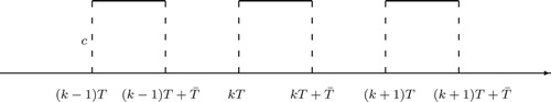
$T>\overline{T}$: If new sterile mosquitoes are not released often, particularly, not until those sexually active sterile mosquitoes who are released in the previous period of time stop mating, the waiting time for the next release is $T>\overline{T}$. In the meantime, it is clear that if we wait for too long to release sterile mosquitoes, the wild mosquitoes may recover and reoccupy the field so that our control process may have to start over. Thus, in addition, we assume $\overline{T}<T<2\overline{T}$. In such a case, there are c sexually active sterile mosquitoes in the time interval $\left[\right(k-1)T,(k-1)T+\overline{T})$, and no sexually active sterile mosquitoes during the time period of $(k-1)T+\overline{T}\le t<kT$, for $k\ge 1$. A schematic diagram for the release function is given in Figure 1. Function $g\left(t\right)$ then becomes a piecewise step function as (7) $g\left(t\right)=\left\{\begin{array}{ll}c,& (k-1)T\le t<(k-1)T+\overline{T},\\ 0,& (k-1)T+\overline{T}\le t<kT,\end{array}\right.$(7) for $k=1,2,\dots$.

Figure 1. Schematic graph of release function $g\left(t\right)$ with the assumption $\overline{T}<T<2\overline{T}$ for $k\ge 1$.

$T<\overline{T}$: On the other hand, suppose that new sterile mosquitoes are released before the previously released sterile mosquitoes become sexually inactive such that $T<\overline{T}$. Then it is clear that if the release is too often with $pT<\overline{T}$, where the positive integer $p\ge 2$, function $g\left(t\right)$ approaches infinity as t goes to infinity, which certainly wastes resources. Thus we assume $T<\overline{T}<2T$. In this case, since the sterile mosquitoes who are released at kT are still sexually active at $(k+1)T$, the number of sterile mosquitoes at $(k+1)T$ is $2c$, for $k\ge 1$. After time reaches $kT+\overline{T},c$ sterile mosquitoes are no longer sexually active and thus no longer play a role in the mating. Then the number of sexually active sterile mosquitoes becomes c again until new sterile mosquitoes are released at $(k+1)T$. The schematic diagram for the release function is shown in Figure 2.

Figure 2. Schematic graph of release function $g\left(t\right)$ for $k\ge 2$ with the assumption $T<\overline{T}<2T$.

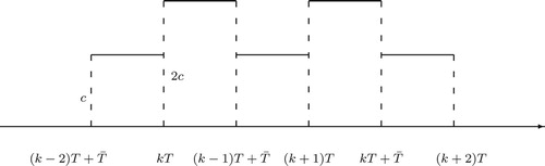
With such a release strategy, function $g\left(t\right)$ has the following form: (8) $g\left(t\right)=\left\{\begin{array}{ll}c,& 0\le t<T,\\ 2c,& kT\le t<(k-1)T+\overline{T},\\ c,& (k-1)T+\overline{T}\le t<(k+1)T,\end{array}\right.$(8) for $k=1,2,\dots$.

Now for the given function g in (8(8) $g\left(t\right)=\left\{\begin{array}{ll}c,& 0\le t<T,\\ 2c,& kT\le t<(k-1)T+\overline{T},\\ c,& (k-1)T+\overline{T}\le t<(k+1)T,\end{array}\right.$(8) ), we have $\underset{t\in (0,\mathrm{\infty })}{inf}g\left(t\right)=c$. Thus it follows from Theorem 2.2 that if $c\ge g^{\ast }$, the trivial equilibrium $E_0=0$ of (4(4) $\frac{\mathrm{d}w\left(t\right)}{\mathrm{d}t}=\frac{a{e}^{-{\mu }_0\tau }{w}^2(t-\tau )}{w(t-\tau )+g(t-\tau )}-\left(\mu +\xi (w\left(t\right)+g\left(t\right))\right)w\left(t\right),$(4) ) is globally uniformly asymptotically stable. However, for the given function in (7(7) $g\left(t\right)=\left\{\begin{array}{ll}c,& (k-1)T\le t<(k-1)T+\overline{T},\\ 0,& (k-1)T+\overline{T}\le t<kT,\end{array}\right.$(7) ), we have $\underset{t\ge 0}{inf}g\left(t\right)=0$. Theorem 2.2 then does not apply. For certain initial values of $y\left(0\right)$, even with a large amount of releases c, we cannot ensure $\underset{t\to \mathrm{\infty }}{lim}w(t,g,t_0,\phi )=0$.

We provide below a numerical example to confirm our assertions.

Example 3.1

Given the following vital parameters of mosquitoes (9) $a=50,{\mu }_0=0.3,\mu =0.2,\xi =0.1,\tau =9,$(9) and the sexual lifespan of sterile mosquitoes $\overline{T}=5.5$, we have the threshold $g^{\ast }=7.4304$.

We first assume $T=10>\overline{T}$. With the fixed initial value $y\left(0\right)=4$, we vary the release amounts c = 10, 15, 20, respectively, all greater than $g^{\ast }$. We have $\underset{t\to \mathrm{\infty }}{lim}w(t,g,t_0,\phi )>0$ for all of the cases as shown in the left figure in Figure 3.

Figure 3. The parameters are given in (9(9) $a=50,{\mu }_0=0.3,\mu =0.2,\xi =0.1,\tau =9,$(9) ) such that the release threshold $g^{\ast }=7.4304$. We assume that the sterile mosquitoes are released at T = 10 and T = 5, respectively. The solutions for T = 10 are shown in the left figure, where we let c = 10, 15, and 20, and the corresponding solutions are in blue, red, and black, respectively, none of which approaches zero. The solutions for T = 5 are shown in the right figure, where we have c = 10 and $y\left(0\right)=4$, 8, 14, and the corresponding solutions are in blue, red, and black, respectively, all of which approach zero.

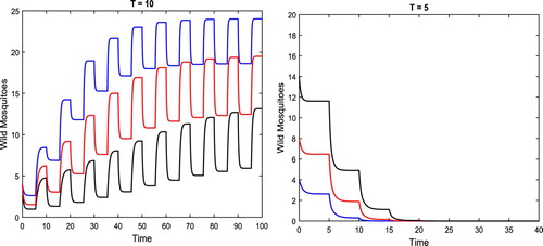
If $T=5<\overline{T}$, on the other hand, when $c=10>g^{\ast }$, the trivial equilibrium $E_0=0$ of (4(4) $\frac{\mathrm{d}w\left(t\right)}{\mathrm{d}t}=\frac{a{e}^{-{\mu }_0\tau }{w}^2(t-\tau )}{w(t-\tau )+g(t-\tau )}-\left(\mu +\xi (w\left(t\right)+g\left(t\right))\right)w\left(t\right),$(4) ) becomes globally uniformly asymptotically stable as shown in the right figure in Figure 3.

The frequency of releases, that is, how often the sterile mosquitoes are released, plays an important role in the control of wild mosquitoes. In this example, as the sterile mosquitoes are released less often, particularly, not before the previously released become sexually inactive, with T = 10 greater than the sexual lifespan $\overline{T}=5$ shown in the left figure in Figure 3, the solutions for the wild mosquitoes are all kept positive for the release amount even reaching c = 20. As the sterile mosquitoes are released more often before the previously released lose their mating ability with $T=5<\overline{T}$, all solutions for the wild mosquitoes vanish as time goes on as shown in the right figure in Figure 3.

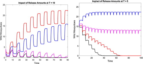
We can also compare the two release strategies with T = 10 and T = 5, respectively. While increasing the release amounts of the sterile mosquitoes can both suppress the wild mosquitoes, the impact is different. In the following, we keep all parameters fixed as in (9(9) $a=50,{\mu }_0=0.3,\mu =0.2,\xi =0.1,\tau =9,$(9) ). For $T=10>\overline{T}$, we gradually increase the release amount c from $12,18,25$, to 28. The corresponding solutions w with the same initial values gradually change from staying positive to approaching zero as shown in the left figure in Figure 4. For $T=5<\overline{T}$, as we gradually increase c from $3,4,5,6$, to 7, the corresponding solutions w with the same initial values change from staying positive to approaching the origin as shown in the right figure in Figure 4. With the quicker release T = 5, not only the wild mosquitoes are suppressed down more quickly, the needed amounts of released sterile mosquitoes are also significantly reduced.

Figure 4. Parameters are given in (9(9) $a=50,{\mu }_0=0.3,\mu =0.2,\xi =0.1,\tau =9,$(9) ) and the release times are T = 10 and T = 5, respectively. The results with different release amounts of sterile mosquitoes c are compared. For T = 10, we gradually increase c from $12,18,25$, to 28. The corresponding solutions w with the same initial values are shown in the left figure. For T = 5, the release amounts c are gradually increased from $3,5,6$, to 7. The corresponding solutions w with the same initial values are shown in the right figure.

4. More model equations derivations and their dynamics

In general, modelling of populations and epidemics with impulsive releases of engineered mosquitoes is challenging and their dynamics can be complex [10,14,21]. Under certain conditions, we convert the models, based on equation (4(4) $\frac{\mathrm{d}w\left(t\right)}{\mathrm{d}t}=\frac{a{e}^{-{\mu }_0\tau }{w}^2(t-\tau )}{w(t-\tau )+g(t-\tau )}-\left(\mu +\xi (w\left(t\right)+g\left(t\right))\right)w\left(t\right),$(4) ), with periodic and impulse releases explicitly to new systems with different expressions in different time intervals. We consider a few particular cases as follows.

4.1. Release less often with $\overline{T}<T$

We assume the sterile mosquitoes are released less often such that $T>\overline{T}$, and further assume (10) $\overline{T}<\tau <T<\overline{T}+\tau .$(10) Define the translation map $P_{\tau }\left(t\right):=t-\tau$. Then more equation settings can be derived as follows.

On interval $[kT,kT+\overline{T}):=I,g\left(t\right)=c$. Decompose $I=I_1\cup I_2$ where $I_1:=[kT,(k-1)T+\overline{T}+\tau )$ and $I_2:=\left[\right(k-1)T+\overline{T}+\tau ,kT+\overline{T})$. If $t\in I_1$, then it follows from $(k-1)T<(k-1)T+T-\tau =kT-\tau \le t-\tau <(k-1)T+\overline{T}$ that $P_{\tau }\left(I_1\right)\subset \left(\right(k-1)T,(k-1)T+\overline{T})$ and thus $g(t-\tau )=c$. If $t\in I_2$, then $(k-1)T+\overline{T}\le t-\tau <kT+\overline{T}-\tau <KT.$ Thus $P_{\tau }\left(I_2\right)\subset \left[\right(k-1)T+\overline{T},kT)$ and $g(t-\tau )=0$.

On the other hand, on interval $(kT+\overline{T},(k+1\left)T\right):=II$, we have $g\left(t\right)=0$. Decompose $II=I{I}_1\cup I{I}_2$ where $I{I}_1:=(kT+\overline{T},kT+\tau ]$ and $I{I}_2:=(kT+\tau ,(k+1\left)T\right]$. If $t\in I{I}_1$, then $(k-1)T+\overline{T}<(k-1)T+\overline{T}+T-\tau =kT+\overline{T}-\tau <t-\tau \le kT.$ Thus $P_{\tau }\left(I{I}_1\right)\subset \left(\right(k-1)T+\overline{T},kT)$ such that $g(t-\tau )=0$. If $t\in I{I}_2$, then $kT<t-\tau \le kT-\tau =kT+\overline{T}+T-(\overline{T}+\tau )<kT+\overline{T}.$ Thus, $P_{\tau }\left(I{I}_2\right)\subset (kT,(k-1)T+\overline{T})$ and then $g(t-\tau )=c$.

The possible cases with $\overline{T}<\tau <T<\overline{T}+\tau$ can be summarized in Table 1. Substituting the values of $g\left(t\right)$ and $g(t-\tau )$ from Table 1 into equation (4(4) $\frac{\mathrm{d}w\left(t\right)}{\mathrm{d}t}=\frac{a{e}^{-{\mu }_0\tau }{w}^2(t-\tau )}{w(t-\tau )+g(t-\tau )}-\left(\mu +\xi (w\left(t\right)+g\left(t\right))\right)w\left(t\right),$(4) ) for different time intervals, we have

Table 1. Summary table for $\overline{T}<\tau <T<\overline{T}+\tau$.

	$kT\le t<kT+\overline{T}$
	$kT\le t<(k-1)T+\overline{T}+\tau$	$(k-1)T+\overline{T}+\tau \le t<kT+\overline{T}$
$g\left(t\right)$	c
$g(t-\tau )$	c	0
	$kT+\overline{T}<t\le (k+1)T$
	$kT+\overline{T}<t\le kT+\tau$	$kT+\tau <t<(k+1)T$
$g\left(t\right)$	0
$g(t-\tau )$	0	c

(11) $\begin{array}{rl}& \frac{\mathrm{d}w\left(t\right)}{\mathrm{d}t}\\ & =\left\{\begin{array}{ll}a{e}^{-{\mu }_0\tau }w(t-\tau )-\left(\mu +\xi \left(w\left(t\right)+c\right)\right)w\left(t\right),& 0<t\le \overline{T},\\ a{e}^{-{\mu }_0\tau }w(t-\tau )-\left(\mu +\xi w\left(t\right)\right)w\left(t\right),& \overline{T}<t\le \tau ,\\ \frac{a{e}^{-{\mu }_0\tau }{w}^2(t-\tau )}{w(t-\tau )+c}-\left(\mu +\xi w\left(t\right)\right)w\left(t\right),& \tau <t<T,\\ \frac{a{e}^{-{\mu }_0\tau }{w}^2(t-\tau )}{w(t-\tau )+c}-\left(\mu +\xi \left(w\left(t\right)+c\right)\right)w\left(t\right),& kT\le t<(k-1)T+\overline{T}+\tau ,\\ a{e}^{-{\mu }_0\tau }w(t-\tau )-\left(\mu +\xi \left(w\left(t\right)+c\right)\right)w\left(t\right),& (k-1)T+\overline{T}+\tau \le t<kT+\overline{T},\\ a{e}^{-{\mu }_0\tau }w(t-\tau )-\left(\mu +\xi w\left(t\right)\right)w\left(t\right),& kT+\overline{T}<t\le kT+\tau ,\\ \frac{a{e}^{-{\mu }_0\tau }{w}^2(t-\tau )}{w(t-\tau )+c}-\left(\mu +\xi w\left(t\right)\right)w\left(t\right),& kT+\tau <t<(k+1)T,\end{array}\right.\end{array}$(11) where $k\ge 1$.

We now show the existence of periodic solutions of system (11(11) $\begin{array}{rl}& \frac{\mathrm{d}w\left(t\right)}{\mathrm{d}t}\\ & =\left\{\begin{array}{ll}a{e}^{-{\mu }_0\tau }w(t-\tau )-\left(\mu +\xi \left(w\left(t\right)+c\right)\right)w\left(t\right),& 0<t\le \overline{T},\\ a{e}^{-{\mu }_0\tau }w(t-\tau )-\left(\mu +\xi w\left(t\right)\right)w\left(t\right),& \overline{T}<t\le \tau ,\\ \frac{a{e}^{-{\mu }_0\tau }{w}^2(t-\tau )}{w(t-\tau )+c}-\left(\mu +\xi w\left(t\right)\right)w\left(t\right),& \tau <t<T,\\ \frac{a{e}^{-{\mu }_0\tau }{w}^2(t-\tau )}{w(t-\tau )+c}-\left(\mu +\xi \left(w\left(t\right)+c\right)\right)w\left(t\right),& kT\le t<(k-1)T+\overline{T}+\tau ,\\ a{e}^{-{\mu }_0\tau }w(t-\tau )-\left(\mu +\xi \left(w\left(t\right)+c\right)\right)w\left(t\right),& (k-1)T+\overline{T}+\tau \le t<kT+\overline{T},\\ a{e}^{-{\mu }_0\tau }w(t-\tau )-\left(\mu +\xi w\left(t\right)\right)w\left(t\right),& kT+\overline{T}<t\le kT+\tau ,\\ \frac{a{e}^{-{\mu }_0\tau }{w}^2(t-\tau )}{w(t-\tau )+c}-\left(\mu +\xi w\left(t\right)\right)w\left(t\right),& kT+\tau <t<(k+1)T,\end{array}\right.\end{array}$(11) ) and thus of equation (4(4) $\frac{\mathrm{d}w\left(t\right)}{\mathrm{d}t}=\frac{a{e}^{-{\mu }_0\tau }{w}^2(t-\tau )}{w(t-\tau )+g(t-\tau )}-\left(\mu +\xi (w\left(t\right)+g\left(t\right))\right)w\left(t\right),$(4) ).

Write $\begin{array}{rl}{f}_1\left(w\right(t),w(t-\tau \left)\right)& :=\frac{a{e}^{-{\mu }_0\tau }{w}^2(t-\tau )}{w(t-\tau )+c}-\left(\mu +\xi \left(w\left(t\right)+c\right)\right)w\left(t\right),\\ f_2\left(w\right(t),w(t-\tau \left)\right)& :=\left(a{e}^{-{\mu }_0\tau }w\right(t-\tau )-\left(\mu +\xi \left(w\left(t\right)+c\right)\right)w(t),\\ f_3\left(w\right(t),w(t-\tau \left)\right)& :=a{e}^{-{\mu }_0\tau }w(t-\tau )-\left(\mu +\xi w\left(t\right)\right)w\left(t\right),\\ f_4\left(w\right(t),w(t-\tau \left)\right)& :=\frac{a{e}^{-{\mu }_0\tau }{w}^2(t-\tau )}{w(t-\tau )+c}-\left(\mu +\xi w\left(t\right)\right)w\left(t\right).\end{array}$ Assume $0<c<g^{\ast }$, where $g^{\ast }$ is given in (6(6) $g^{\ast }=\frac{{\left(a{e}^{-{\mu }_0\tau }-\mu \right)}^2}{4a\xi e^{-{\mu }_0\tau }}.$(6) ). Then we have $\begin{array}{rl}{f}_1(w,w)& =\frac{\left(a{e}^{-{\mu }_0\tau }w-(\mu +\xi (w+c\left)\right(w+c)\right)w}{w+c}=\frac{\xi w\left(w_1^{+}-w\right)\left(w-w_1^{-}\right)}{w+c},\\ f_2(w,w)& =\left(a{e}^{-{\mu }_0\tau }-\mu -\xi (w+c)\right)w=\xi w\left(w_2^{+}-w\right),\\ f_3(w,w)& =\left(a{e}^{-{\mu }_0\tau }-\mu -\xi w\right)w=\xi w\left(w_3^{+}-w\right),\\ f_4(w,w)& =\frac{\left(a{e}^{-{\mu }_0\tau }w-(\mu +\xi w)(w+c)\right)w}{w+c}=\frac{\xi w\left(w_4^{+}-w\right)\left(w-w_4^{-}\right)}{w+c},\end{array}$ where $\begin{array}{rl}{w}_1^{\pm }& =-c+\frac{a{e}^{-{\mu }_0\tau }-\mu }{2\xi }\left(1\pm \sqrt{1-\frac{c}{g^{\ast }}}\right)>0,\\ w_2^{+}& =-c+\frac{a{e}^{-{\mu }_0\tau }-\mu }{\xi }>0,\\ w_3^{+}& =\frac{a{e}^{-{\mu }_0\tau }-\mu }{\xi }>0,\\ w_4^{\pm }& =-c+\frac{a{e}^{-{\mu }_0\tau }-\mu +\xi c}{2\xi }\left(1\pm \sqrt{1-\frac{c}{g^{\ast }}{\left(\frac{a{e}^{-{\mu }_0\tau }-\mu }{a{e}^{-{\mu }_0\tau }-\mu +\xi c}\right)}^2}\right)>0.\end{array}$ It is easy to check that $w_2^{+}<w_3^{+},w_1^{+}<w_4^{+}$, and $\begin{array}{rl}{w}_1^{+}+w_1^{-}& =\frac{a_0{e}^{-{\mu }_{0}r}-\mu -2\xi c}{\xi },w_4^{+}+w_4^{-}=\frac{a_0{e}^{-{\mu }_{0}r}-\mu -\xi c}{\xi },\\ w_4^{+}{w}_4^{-}& =\frac{\mu c}{\xi }<\frac{(\mu +\xi c)c}{\xi }=w_1^{+}{w}_1^{-}.\end{array}$ It then follows that (12) $w_4^{-}<w_1^{-}<w_1^{+}<w_4^{+}<w_2^{+}<w_3^{+}.$(12) With these preparations, we have the following existence of periodic solutions for system (11(11) $\begin{array}{rl}& \frac{\mathrm{d}w\left(t\right)}{\mathrm{d}t}\\ & =\left\{\begin{array}{ll}a{e}^{-{\mu }_0\tau }w(t-\tau )-\left(\mu +\xi \left(w\left(t\right)+c\right)\right)w\left(t\right),& 0<t\le \overline{T},\\ a{e}^{-{\mu }_0\tau }w(t-\tau )-\left(\mu +\xi w\left(t\right)\right)w\left(t\right),& \overline{T}<t\le \tau ,\\ \frac{a{e}^{-{\mu }_0\tau }{w}^2(t-\tau )}{w(t-\tau )+c}-\left(\mu +\xi w\left(t\right)\right)w\left(t\right),& \tau <t<T,\\ \frac{a{e}^{-{\mu }_0\tau }{w}^2(t-\tau )}{w(t-\tau )+c}-\left(\mu +\xi \left(w\left(t\right)+c\right)\right)w\left(t\right),& kT\le t<(k-1)T+\overline{T}+\tau ,\\ a{e}^{-{\mu }_0\tau }w(t-\tau )-\left(\mu +\xi \left(w\left(t\right)+c\right)\right)w\left(t\right),& (k-1)T+\overline{T}+\tau \le t<kT+\overline{T},\\ a{e}^{-{\mu }_0\tau }w(t-\tau )-\left(\mu +\xi w\left(t\right)\right)w\left(t\right),& kT+\overline{T}<t\le kT+\tau ,\\ \frac{a{e}^{-{\mu }_0\tau }{w}^2(t-\tau )}{w(t-\tau )+c}-\left(\mu +\xi w\left(t\right)\right)w\left(t\right),& kT+\tau <t<(k+1)T,\end{array}\right.\end{array}$(11) ) and thus for equation (4(4) $\frac{\mathrm{d}w\left(t\right)}{\mathrm{d}t}=\frac{a{e}^{-{\mu }_0\tau }{w}^2(t-\tau )}{w(t-\tau )+g(t-\tau )}-\left(\mu +\xi (w\left(t\right)+g\left(t\right))\right)w\left(t\right),$(4) ).

Theorem 4.1

Assume $0<c<g^{\ast }$ with $g^{\ast }$ given in (6(6) $g^{\ast }=\frac{{\left(a{e}^{-{\mu }_0\tau }-\mu \right)}^2}{4a\xi e^{-{\mu }_0\tau }}.$(6) ). Then for the periodic release function $g\left(t\right)$ given in (7(7) $g\left(t\right)=\left\{\begin{array}{ll}c,& (k-1)T\le t<(k-1)T+\overline{T},\\ 0,& (k-1)T+\overline{T}\le t<kT,\end{array}\right.$(7) ), system (11(11) $\begin{array}{rl}& \frac{\mathrm{d}w\left(t\right)}{\mathrm{d}t}\\ & =\left\{\begin{array}{ll}a{e}^{-{\mu }_0\tau }w(t-\tau )-\left(\mu +\xi \left(w\left(t\right)+c\right)\right)w\left(t\right),& 0<t\le \overline{T},\\ a{e}^{-{\mu }_0\tau }w(t-\tau )-\left(\mu +\xi w\left(t\right)\right)w\left(t\right),& \overline{T}<t\le \tau ,\\ \frac{a{e}^{-{\mu }_0\tau }{w}^2(t-\tau )}{w(t-\tau )+c}-\left(\mu +\xi w\left(t\right)\right)w\left(t\right),& \tau <t<T,\\ \frac{a{e}^{-{\mu }_0\tau }{w}^2(t-\tau )}{w(t-\tau )+c}-\left(\mu +\xi \left(w\left(t\right)+c\right)\right)w\left(t\right),& kT\le t<(k-1)T+\overline{T}+\tau ,\\ a{e}^{-{\mu }_0\tau }w(t-\tau )-\left(\mu +\xi \left(w\left(t\right)+c\right)\right)w\left(t\right),& (k-1)T+\overline{T}+\tau \le t<kT+\overline{T},\\ a{e}^{-{\mu }_0\tau }w(t-\tau )-\left(\mu +\xi w\left(t\right)\right)w\left(t\right),& kT+\overline{T}<t\le kT+\tau ,\\ \frac{a{e}^{-{\mu }_0\tau }{w}^2(t-\tau )}{w(t-\tau )+c}-\left(\mu +\xi w\left(t\right)\right)w\left(t\right),& kT+\tau <t<(k+1)T,\end{array}\right.\end{array}$(11) ) and thus equation (4(4) $\frac{\mathrm{d}w\left(t\right)}{\mathrm{d}t}=\frac{a{e}^{-{\mu }_0\tau }{w}^2(t-\tau )}{w(t-\tau )+g(t-\tau )}-\left(\mu +\xi (w\left(t\right)+g\left(t\right))\right)w\left(t\right),$(4) ) has a piecewise $C^1$-smooth and continuous T- periodic solution satisfying $w_1^{+}\le w\left(t\right)\le w_3^{+}$ for $t\ge T$.

The proof is given in Appendix.

We give an example below to confirm the results in Theorem 4.1.

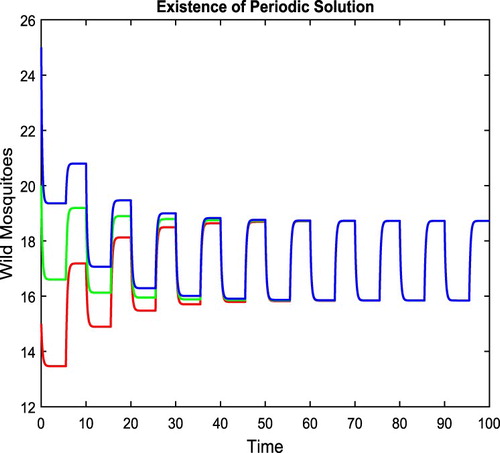
Example 4.1

Give the following vital parameters of mosquitoes (13) $a=20,{\mu }_0=0.3,\mu =0.2,\xi =0.1,\tau =9,$(13) such that $g^{\ast }=5.1637$. We then let $c=5<g^{\ast },\overline{T}=5.5$, and T = 10 such that condition (10(10) $\overline{T}<\tau <T<\overline{T}+\tau .$(10) ) holds. With such parameters, $w_1^{+}=8.2477,w_3^{+}=\mathrm{22.4913.}$ Thus there exists a periodic solution with period T = 10, bounded below by $w_1^{+}$ and above by $w_3^{+}$, as shown in Figure 5. Although we have not been able to prove the stability of this periodic solution, its stability seems shown in the figure.

Figure 5. With parameters given in (13(13) $a=20,{\mu }_0=0.3,\mu =0.2,\xi =0.1,\tau =9,$(13) ), $c=5<g^{\ast }=5.1637$, and condition (10(10) $\overline{T}<\tau <T<\overline{T}+\tau .$(10) ) holds. There exists a positive 10-periodic solution, between $w_1^{+}=8.2477$ and $w_3^{+}=22.4913$, as shown in the figure.

4.2. Release more often with $T<\overline{T}$

For the case of $T<\overline{T}$, if we further assume (14) $T<\overline{T}<\tau <2T,\tau +\overline{T}<3T.$(14) System (4(4) $\frac{\mathrm{d}w\left(t\right)}{\mathrm{d}t}=\frac{a{e}^{-{\mu }_0\tau }{w}^2(t-\tau )}{w(t-\tau )+g(t-\tau )}-\left(\mu +\xi (w\left(t\right)+g\left(t\right))\right)w\left(t\right),$(4) ) can also be set more explicitly as follows.

First, for $t\in [0,T)$, we have $g\left(t\right)=c$ and $g(t-\tau )=0$, and for $t\in [T,\overline{T})$, we have $g\left(t\right)=2c$ and $g(t-\tau )=0$.

For $k\ge 2$, on interval $\left[\right(k+1)T,kT+\overline{T}):=J_1$, we have $g\left(t\right)=2c$. If $t\in J_1$, it follows from $(k+1)T-\tau -((k-2)T+\overline{T})=3T-(\tau +\overline{T})>0$ and $kT+\overline{T}-\tau -kT=\overline{T}-\tau <0$ that $P_{\tau }\left(J_1\right)\subset \left(\right(k-2)T+\overline{T},kT]$ and thus $g(t-\tau )=c$ for $t\in J_1$.

Write intervals $J_2:=[kT+\overline{T},(k+2\left)T\right),J_{2a}:=[kT+\overline{T},kT+\tau ),J_{2b}:=[kT+\tau ,(k-1)T+\overline{T}+\tau )$, and $J_{2c}:=\left(\right(k-1)T+\overline{T}+\tau ,(k+2\left)T\right)$. Then $g\left(t\right)=c$ on $J_2$, and it follows from $kT+\overline{T}-\tau -\left(\right(k-2)T+\overline{T})=2T-\tau >0$ and $kT+\tau -\tau =kT$ that $P_{\tau }\left(J_{2a}\right)\subset \left(\right(k-2)T+\overline{T},kT)$ and thus $g(t-\tau )=c$ for $t\in J_{2a}$.

Since $P_{\tau }\left(J_{2b}\right)=[kT,(k-1)T+\overline{T})$, we have $g(t-\tau )=2c$ on $J_{2b}$. It follows from $(k-1)T+\overline{T}+\tau -\tau =(k-1)T+\overline{T}$ and $(k+2)T-\tau =(k+1)T-(\tau -T)<(k+1)T$ that $P_{\tau }\left(J_{2c}\right)\subset \left(\right(k-1)T+\overline{T},(k+1\left)T\right)$ and thus $g(t-\tau )=c$. We summarize the possible cases with $T<\overline{T}<\tau <2T$ and $\tau +\overline{T}<3T$ in Table 2. Substituting the values of $g\left(t\right)$ and $g(t-\tau )$ from Table 2 into equation (4(4) $\frac{\mathrm{d}w\left(t\right)}{\mathrm{d}t}=\frac{a{e}^{-{\mu }_0\tau }{w}^2(t-\tau )}{w(t-\tau )+g(t-\tau )}-\left(\mu +\xi (w\left(t\right)+g\left(t\right))\right)w\left(t\right),$(4) ) in different time intervals, we have

Table 2. Summary table for $T<\overline{T}<\tau <2T$ and $\tau +\overline{T}<3T$.

	$0<t\le T$	$T\le t<\overline{T}$	$\overline{T}<t\le 2T$
			$\overline{T}<t\le \tau$	$\tau <t\le 2T$
$g\left(t\right)$	c	2c	c
$g(t-\tau )$	0	0	0	c
	For $k\ge 1$:
	$(k+1)T\le t<kT+\overline{T}$
$g\left(t\right)$	2c
$g(t-\tau )$	c
	$kT+\overline{T}\le t<(k+2)T$
	$kT+\overline{T}\le t<kT+\tau$	$kT+\tau \le t<(k-1)T+\overline{T}+\tau$	$(k-1)T+\overline{T}+\tau \le t<(k+2)T$
$g\left(t\right)$	c
$g(t-\tau )$	c	2c	c

(15) $\begin{array}{rl}& \frac{\mathrm{d}w\left(t\right)}{\mathrm{d}t}\\ & =\left\{\begin{array}{ll}a{e}^{-{\mu }_0\tau }w(t-\tau )-\left(\mu +\xi \left(w\left(t\right)+c\right)\right)w\left(t\right),& 0<t\le T,\\ a{e}^{-{\mu }_0\tau }w(t-\tau )-\left(\mu +\xi \left(w\left(t\right)+2c\right)\right)w\left(t\right),& T\le t<\overline{T},\\ a{e}^{-{\mu }_0\tau }w(t-\tau )-\left(\mu +\xi \left(w\left(t\right)+c\right)\right)w\left(t\right),& \overline{T}<t\le \tau ,\\ \frac{a{e}^{-{\mu }_0\tau }{w}^2(t-\tau )}{w(t-\tau )+c}-\left(\mu +\xi \left(w\left(t\right)+c\right)\right)w\left(t\right),& \tau <t\le 2T,\\ \frac{a{e}^{-{\mu }_0\tau }{w}^2(t-\tau )}{w(t-\tau )+c}-\left(\mu +\xi \left(w\left(t\right)+2c\right)\right)w\left(t\right),& (k+1)T\le t<kT+\overline{T},\\ \frac{a{e}^{-{\mu }_0\tau }{w}^2(t-\tau )}{w(t-\tau )+c}-\left(\mu +\xi \left(w\left(t\right)+c\right)\right)w\left(t\right),& kT+\overline{T}\le t<kT+\tau ,\\ \frac{a{e}^{-{\mu }_0\tau }{w}^2(t-\tau )}{w(t-\tau )+2c}-\left(\mu +\xi \left(w\left(t\right)+c\right)\right)w\left(t\right),& kT+\tau \le t<(k-1)T+\overline{T}+\tau ,\\ \frac{a{e}^{-{\mu }_0\tau }{w}^2(t-\tau )}{w(t-\tau )+c}-\left(\mu +\xi \left(w\left(t\right)+c\right)\right)w\left(t\right),& (k-1)T+\overline{T}+\tau \le t<(k+2)T,\end{array}\right.\end{array}$(15) where $k\ge 1$.

To show the existence of periodic solutions for system (15(15) $\begin{array}{rl}& \frac{\mathrm{d}w\left(t\right)}{\mathrm{d}t}\\ & =\left\{\begin{array}{ll}a{e}^{-{\mu }_0\tau }w(t-\tau )-\left(\mu +\xi \left(w\left(t\right)+c\right)\right)w\left(t\right),& 0<t\le T,\\ a{e}^{-{\mu }_0\tau }w(t-\tau )-\left(\mu +\xi \left(w\left(t\right)+2c\right)\right)w\left(t\right),& T\le t<\overline{T},\\ a{e}^{-{\mu }_0\tau }w(t-\tau )-\left(\mu +\xi \left(w\left(t\right)+c\right)\right)w\left(t\right),& \overline{T}<t\le \tau ,\\ \frac{a{e}^{-{\mu }_0\tau }{w}^2(t-\tau )}{w(t-\tau )+c}-\left(\mu +\xi \left(w\left(t\right)+c\right)\right)w\left(t\right),& \tau <t\le 2T,\\ \frac{a{e}^{-{\mu }_0\tau }{w}^2(t-\tau )}{w(t-\tau )+c}-\left(\mu +\xi \left(w\left(t\right)+2c\right)\right)w\left(t\right),& (k+1)T\le t<kT+\overline{T},\\ \frac{a{e}^{-{\mu }_0\tau }{w}^2(t-\tau )}{w(t-\tau )+c}-\left(\mu +\xi \left(w\left(t\right)+c\right)\right)w\left(t\right),& kT+\overline{T}\le t<kT+\tau ,\\ \frac{a{e}^{-{\mu }_0\tau }{w}^2(t-\tau )}{w(t-\tau )+2c}-\left(\mu +\xi \left(w\left(t\right)+c\right)\right)w\left(t\right),& kT+\tau \le t<(k-1)T+\overline{T}+\tau ,\\ \frac{a{e}^{-{\mu }_0\tau }{w}^2(t-\tau )}{w(t-\tau )+c}-\left(\mu +\xi \left(w\left(t\right)+c\right)\right)w\left(t\right),& (k-1)T+\overline{T}+\tau \le t<(k+2)T,\end{array}\right.\end{array}$(15) ), we first define (16) $g_1^{\ast }=\frac{{\left(a{e}^{-{\mu }_0\tau }-\mu \right)}^2}{4\xi \left(2a{e}^{-{\mu }_0\tau }-\mu \right)},g_2^{\ast }=\frac{{\left(a{e}^{-{\mu }_0\tau }-\mu \right)}^2}{4\xi \left(2a{e}^{-{\mu }_0\tau }\right)}.$(16) It follows from (5(5) $a{e}^{-{\mu }_0\tau }-\mu >0.$(5) ) that $2a^{-{\mu }_0\tau }-\mu =a^{-{\mu }_0\tau }+a^{-{\mu }_0\tau }-\mu >a^{-{\mu }_0\tau },$ and thus $g_2^{\ast }<g_1^{\ast }<g^{\ast }.$ Write $\begin{array}{rl}{f}_1\left(w\right(t),w(t-r\left)\right)& :=\frac{a{e}^{-{\mu }_{0}r}{w}^2(t-r)}{w(t-r)+c}-(\mu +\xi (w+2c))w,\\ f_2\left(w\right(t),w(t-r\left)\right)& :=\frac{a{e}^{-{\mu }_{0}r}{w}^2(t-r)}{w(t-r)+c}-(\mu +\xi (w+c))w,\\ f_3\left(w\right(t),w(t-r\left)\right)& :=\frac{a{e}^{-{\mu }_{0}r}{w}^2(t-r)}{w(t-r)+2c}-(\mu +\xi (w+c))w.\end{array}$ Then $\begin{array}{rl}{f}_1(w,w)& =\frac{\left(a{e}^{-{\mu }_{0}r}w-(\mu +\xi (w+2c))(w+c)\right)w}{w+c}=\frac{\xi w\left(w_1^{+}-w\right)\left(w-w_1^{-}\right)}{w+c},\\ f_2(w,w)& =\frac{\left(a{e}^{-{\mu }_{0}r}w-(\mu +\xi (w+c))(w+c)\right)w}{w+c}=\frac{\xi w\left(w_2^{+}-w\right)\left(w-w_2^{-}\right)}{w+c},\\ f_3(w,w)& =\frac{\left(a{e}^{-{\mu }_{0}r}w-(\mu +\xi (w+c))(w+2c)\right)w}{w+2c}=\frac{\xi w\left(w_3^{+}-w\right)\left(w-w_3^{-}\right)}{w+2c},\end{array}$ where $\begin{array}{rl}{w}_1^{\pm }& =-2c+\frac{a{e}^{-{\mu }_0\tau }-\mu +\xi c}{2\xi }\left(1\pm \sqrt{1-\frac{c}{g_1^{\ast }}{\left(\frac{a{e}^{-{\mu }_0\tau }-\mu }{a{e}^{-{\mu }_0\tau }-\mu +\xi c}\right)}^2}\right)>0,\\ w_2^{\pm }& =-c+\frac{a{e}^{-{\mu }_0\tau }-\mu }{2\xi }\left(1\pm \sqrt{1-\frac{c}{g_2^{\ast }}}\right)>0,\\ w_3^{\pm }& =-2c+\frac{a{e}^{-{\mu }_0\tau }-\mu +\xi c}{2\xi }\left(1\pm \sqrt{1-\frac{c}{g_2^{\ast }}{\left(\frac{a{e}^{-{\mu }_0\tau }-\mu }{a{e}^{-{\mu }_0\tau }-\mu +\xi c}\right)}^2}\right)>0,\end{array}$ for $0<c<g_2^{\ast }$.

It is easy to check that $w_3^{+}<w_1^{+}<w_2^{+}$. Moreover, since $w_1^{+}{w}_1^{-}=\frac{(\mu +2\xi c)c}{\xi },w_2^{+}{w}_2^{-}=\frac{(\mu +\xi c)c}{\xi },w_3^{+}{w}_3^{-}=\frac{2(\mu +\xi c)c}{\xi },$ it follows that $w_2^{+}{w}_2^{-}<w_1^{+}{w}_1^{-}<w_3^{+}{w}_3^{-},$ and thus (17) $w_2^{-}<w_1^{-}<w_3^{-}<w_3^{+}<w_1^{+}<w_2^{+}.$(17) We have the following existence results the proof of which is also given in Appendix.

Theorem 4.2

Assume that condition (14(14) $T<\overline{T}<\tau <2T,\tau +\overline{T}<3T.$(14) ) holds and $0<c<g_2^{\ast },$ where $g_2^{\ast }$ is given in (16(16) $g_1^{\ast }=\frac{{\left(a{e}^{-{\mu }_0\tau }-\mu \right)}^2}{4\xi \left(2a{e}^{-{\mu }_0\tau }-\mu \right)},g_2^{\ast }=\frac{{\left(a{e}^{-{\mu }_0\tau }-\mu \right)}^2}{4\xi \left(2a{e}^{-{\mu }_0\tau }\right)}.$(16) ). Then system (15(15) $\begin{array}{rl}& \frac{\mathrm{d}w\left(t\right)}{\mathrm{d}t}\\ & =\left\{\begin{array}{ll}a{e}^{-{\mu }_0\tau }w(t-\tau )-\left(\mu +\xi \left(w\left(t\right)+c\right)\right)w\left(t\right),& 0<t\le T,\\ a{e}^{-{\mu }_0\tau }w(t-\tau )-\left(\mu +\xi \left(w\left(t\right)+2c\right)\right)w\left(t\right),& T\le t<\overline{T},\\ a{e}^{-{\mu }_0\tau }w(t-\tau )-\left(\mu +\xi \left(w\left(t\right)+c\right)\right)w\left(t\right),& \overline{T}<t\le \tau ,\\ \frac{a{e}^{-{\mu }_0\tau }{w}^2(t-\tau )}{w(t-\tau )+c}-\left(\mu +\xi \left(w\left(t\right)+c\right)\right)w\left(t\right),& \tau <t\le 2T,\\ \frac{a{e}^{-{\mu }_0\tau }{w}^2(t-\tau )}{w(t-\tau )+c}-\left(\mu +\xi \left(w\left(t\right)+2c\right)\right)w\left(t\right),& (k+1)T\le t<kT+\overline{T},\\ \frac{a{e}^{-{\mu }_0\tau }{w}^2(t-\tau )}{w(t-\tau )+c}-\left(\mu +\xi \left(w\left(t\right)+c\right)\right)w\left(t\right),& kT+\overline{T}\le t<kT+\tau ,\\ \frac{a{e}^{-{\mu }_0\tau }{w}^2(t-\tau )}{w(t-\tau )+2c}-\left(\mu +\xi \left(w\left(t\right)+c\right)\right)w\left(t\right),& kT+\tau \le t<(k-1)T+\overline{T}+\tau ,\\ \frac{a{e}^{-{\mu }_0\tau }{w}^2(t-\tau )}{w(t-\tau )+c}-\left(\mu +\xi \left(w\left(t\right)+c\right)\right)w\left(t\right),& (k-1)T+\overline{T}+\tau \le t<(k+2)T,\end{array}\right.\end{array}$(15) ) has a piecewise $C^1$-smooth and continuous T-periodic solution $w\left(t\right)$ with $w_3^{+}\le w\left(t\right)\le w_2^{+}$ for $t\ge 3T$.

The following example demonstrates the results in Theorem 4.2.

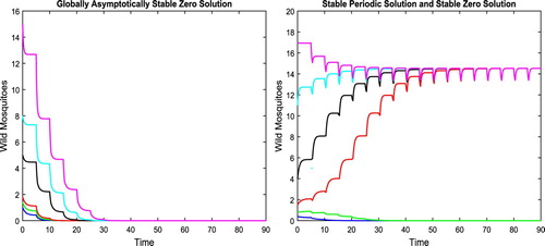
Example 4.2

With the given parameters (18) $a=20,{\mu }_0=0.3,\mu =0.2,\xi =0.1,\tau =7,$(18) we have $g_2^{\ast }=2.5818<g_1^{\ast }=2.6917<g^{\ast }=5.1637$. We then let $\overline{T}=5.5$ and T = 5 such that condition (14(14) $T<\overline{T}<\tau <2T,\tau +\overline{T}<3T.$(14) ) is satisfied. For $c=6>g^{\ast }$, since $\underset{t\in (0,\mathrm{\infty })}{inf}g\left(t\right)=c>g^{\ast }$, the trivial equilibrium is globally uniformly asymptotically stable as shown in the left figure in Figure 6. For $c=2.5<g_2^{\ast }$, we have $w_2^{-}=0.6687<w_3^{-}=1.6918<w_3^{+}=13.2995<w_2^{+}=\mathrm{16.8225.}$ There exists a periodic solution $w\left(t\right)$ with $w_3^{+}\le w\left(t\right)\le w_2^{+}$, which is shown in the right figure in Figure 6. We have not been able to rigorously prove it, but conjecture that this periodic solution $w\left(t\right)$ is asymptotically stable and that, at the same time, there exists another T-periodic solution between $w_2^{-}$ and $w_3^{-}$, which is unstable. We note that this is true in the case without delay.

Figure 6. With parameters given in (18(18) $a=20,{\mu }_0=0.3,\mu =0.2,\xi =0.1,\tau =7,$(18) ), condition (14(14) $T<\overline{T}<\tau <2T,\tau +\overline{T}<3T.$(14) ) holds. For $c=6>g^{\ast }=5.1637$, since $\underset{t\in (0,\mathrm{\infty })}{inf}g\left(t\right)=6>g^{\ast }$, the zero solution is globally asymptotically stable as shown in the left figure. For $c=2.5<g_2^{\ast }=2.5818$, there exists a periodic solution which seems asymptotically stable as shown in the right figure.

5. Concluding remarks

Modeling of populations and epidemics with impulsive releases of engineered mosquitoes is always challenging. Different from those existing methods, adapting the idea and methods in [30,31], we used the model equation (4(4) $\frac{\mathrm{d}w\left(t\right)}{\mathrm{d}t}=\frac{a{e}^{-{\mu }_0\tau }{w}^2(t-\tau )}{w(t-\tau )+g(t-\tau )}-\left(\mu +\xi (w\left(t\right)+g\left(t\right))\right)w\left(t\right),$(4) ) in [31] for the interactive dynamics between wild and sterile mosquito populations as our baseline model and gave brief model descriptions in Section 2. We assumed that the releases of sterile mosquitoes were periodic and impulsive, and considered strategies with different waiting times T based on the sexual lifespan of sterile mosquitoes $\overline{T}$, for releasing sterile mosquitoes, in Section 3. If sterile mosquitoes are released exactly at the end of the sexual lifespan of the sterile mosquitoes, $T=\overline{T}$ and the release function $g\left(t\right)$ becomes constant with which the model dynamics were fully investigated in [31]. We then considered the model dynamics for the cases of $T<\overline{T}$ and $T>\overline{T}$, respectively. We derived explicit expressions for function $g\left(t\right)$. Using a numerical example we demonstrated the fundamental model dynamics with these different release strategies in Example 3.1. When the releases are less often with $T>\overline{T}$, it is difficult to suppress the wild mosquitoes whereas wild mosquitoes can be completely eradicated if the releases are more often with $T<\overline{T}$. We also showed that how the frequency of releases played an important role in determining the effectiveness of the release strategies and that how larger release amounts were needed if we were unable to release the sterile mosquitoes more often and the control measures needed to be compromised. We are unable to give detailed analytic investigations for possible optimal strategies between the releasing amounts and frequencies in this study, but it is one of our future research projects.

Under certain assumptions for the periodic and impulsive releases, we derived model equations explicitly expressed as systems of Filippov-type in (11(11) $\begin{array}{rl}& \frac{\mathrm{d}w\left(t\right)}{\mathrm{d}t}\\ & =\left\{\begin{array}{ll}a{e}^{-{\mu }_0\tau }w(t-\tau )-\left(\mu +\xi \left(w\left(t\right)+c\right)\right)w\left(t\right),& 0<t\le \overline{T},\\ a{e}^{-{\mu }_0\tau }w(t-\tau )-\left(\mu +\xi w\left(t\right)\right)w\left(t\right),& \overline{T}<t\le \tau ,\\ \frac{a{e}^{-{\mu }_0\tau }{w}^2(t-\tau )}{w(t-\tau )+c}-\left(\mu +\xi w\left(t\right)\right)w\left(t\right),& \tau <t<T,\\ \frac{a{e}^{-{\mu }_0\tau }{w}^2(t-\tau )}{w(t-\tau )+c}-\left(\mu +\xi \left(w\left(t\right)+c\right)\right)w\left(t\right),& kT\le t<(k-1)T+\overline{T}+\tau ,\\ a{e}^{-{\mu }_0\tau }w(t-\tau )-\left(\mu +\xi \left(w\left(t\right)+c\right)\right)w\left(t\right),& (k-1)T+\overline{T}+\tau \le t<kT+\overline{T},\\ a{e}^{-{\mu }_0\tau }w(t-\tau )-\left(\mu +\xi w\left(t\right)\right)w\left(t\right),& kT+\overline{T}<t\le kT+\tau ,\\ \frac{a{e}^{-{\mu }_0\tau }{w}^2(t-\tau )}{w(t-\tau )+c}-\left(\mu +\xi w\left(t\right)\right)w\left(t\right),& kT+\tau <t<(k+1)T,\end{array}\right.\end{array}$(11) ) and (15(15) $\begin{array}{rl}& \frac{\mathrm{d}w\left(t\right)}{\mathrm{d}t}\\ & =\left\{\begin{array}{ll}a{e}^{-{\mu }_0\tau }w(t-\tau )-\left(\mu +\xi \left(w\left(t\right)+c\right)\right)w\left(t\right),& 0<t\le T,\\ a{e}^{-{\mu }_0\tau }w(t-\tau )-\left(\mu +\xi \left(w\left(t\right)+2c\right)\right)w\left(t\right),& T\le t<\overline{T},\\ a{e}^{-{\mu }_0\tau }w(t-\tau )-\left(\mu +\xi \left(w\left(t\right)+c\right)\right)w\left(t\right),& \overline{T}<t\le \tau ,\\ \frac{a{e}^{-{\mu }_0\tau }{w}^2(t-\tau )}{w(t-\tau )+c}-\left(\mu +\xi \left(w\left(t\right)+c\right)\right)w\left(t\right),& \tau <t\le 2T,\\ \frac{a{e}^{-{\mu }_0\tau }{w}^2(t-\tau )}{w(t-\tau )+c}-\left(\mu +\xi \left(w\left(t\right)+2c\right)\right)w\left(t\right),& (k+1)T\le t<kT+\overline{T},\\ \frac{a{e}^{-{\mu }_0\tau }{w}^2(t-\tau )}{w(t-\tau )+c}-\left(\mu +\xi \left(w\left(t\right)+c\right)\right)w\left(t\right),& kT+\overline{T}\le t<kT+\tau ,\\ \frac{a{e}^{-{\mu }_0\tau }{w}^2(t-\tau )}{w(t-\tau )+2c}-\left(\mu +\xi \left(w\left(t\right)+c\right)\right)w\left(t\right),& kT+\tau \le t<(k-1)T+\overline{T}+\tau ,\\ \frac{a{e}^{-{\mu }_0\tau }{w}^2(t-\tau )}{w(t-\tau )+c}-\left(\mu +\xi \left(w\left(t\right)+c\right)\right)w\left(t\right),& (k-1)T+\overline{T}+\tau \le t<(k+2)T,\end{array}\right.\end{array}$(15) ) in Section 4. This modelling process and the equation settings are completely different from those with periodic and impulsive releases studied in [10,14,21]. We showed existence of periodic solutions for systems (11(11) $\begin{array}{rl}& \frac{\mathrm{d}w\left(t\right)}{\mathrm{d}t}\\ & =\left\{\begin{array}{ll}a{e}^{-{\mu }_0\tau }w(t-\tau )-\left(\mu +\xi \left(w\left(t\right)+c\right)\right)w\left(t\right),& 0<t\le \overline{T},\\ a{e}^{-{\mu }_0\tau }w(t-\tau )-\left(\mu +\xi w\left(t\right)\right)w\left(t\right),& \overline{T}<t\le \tau ,\\ \frac{a{e}^{-{\mu }_0\tau }{w}^2(t-\tau )}{w(t-\tau )+c}-\left(\mu +\xi w\left(t\right)\right)w\left(t\right),& \tau <t<T,\\ \frac{a{e}^{-{\mu }_0\tau }{w}^2(t-\tau )}{w(t-\tau )+c}-\left(\mu +\xi \left(w\left(t\right)+c\right)\right)w\left(t\right),& kT\le t<(k-1)T+\overline{T}+\tau ,\\ a{e}^{-{\mu }_0\tau }w(t-\tau )-\left(\mu +\xi \left(w\left(t\right)+c\right)\right)w\left(t\right),& (k-1)T+\overline{T}+\tau \le t<kT+\overline{T},\\ a{e}^{-{\mu }_0\tau }w(t-\tau )-\left(\mu +\xi w\left(t\right)\right)w\left(t\right),& kT+\overline{T}<t\le kT+\tau ,\\ \frac{a{e}^{-{\mu }_0\tau }{w}^2(t-\tau )}{w(t-\tau )+c}-\left(\mu +\xi w\left(t\right)\right)w\left(t\right),& kT+\tau <t<(k+1)T,\end{array}\right.\end{array}$(11) ) and (15(15) $\begin{array}{rl}& \frac{\mathrm{d}w\left(t\right)}{\mathrm{d}t}\\ & =\left\{\begin{array}{ll}a{e}^{-{\mu }_0\tau }w(t-\tau )-\left(\mu +\xi \left(w\left(t\right)+c\right)\right)w\left(t\right),& 0<t\le T,\\ a{e}^{-{\mu }_0\tau }w(t-\tau )-\left(\mu +\xi \left(w\left(t\right)+2c\right)\right)w\left(t\right),& T\le t<\overline{T},\\ a{e}^{-{\mu }_0\tau }w(t-\tau )-\left(\mu +\xi \left(w\left(t\right)+c\right)\right)w\left(t\right),& \overline{T}<t\le \tau ,\\ \frac{a{e}^{-{\mu }_0\tau }{w}^2(t-\tau )}{w(t-\tau )+c}-\left(\mu +\xi \left(w\left(t\right)+c\right)\right)w\left(t\right),& \tau <t\le 2T,\\ \frac{a{e}^{-{\mu }_0\tau }{w}^2(t-\tau )}{w(t-\tau )+c}-\left(\mu +\xi \left(w\left(t\right)+2c\right)\right)w\left(t\right),& (k+1)T\le t<kT+\overline{T},\\ \frac{a{e}^{-{\mu }_0\tau }{w}^2(t-\tau )}{w(t-\tau )+c}-\left(\mu +\xi \left(w\left(t\right)+c\right)\right)w\left(t\right),& kT+\overline{T}\le t<kT+\tau ,\\ \frac{a{e}^{-{\mu }_0\tau }{w}^2(t-\tau )}{w(t-\tau )+2c}-\left(\mu +\xi \left(w\left(t\right)+c\right)\right)w\left(t\right),& kT+\tau \le t<(k-1)T+\overline{T}+\tau ,\\ \frac{a{e}^{-{\mu }_0\tau }{w}^2(t-\tau )}{w(t-\tau )+c}-\left(\mu +\xi \left(w\left(t\right)+c\right)\right)w\left(t\right),& (k-1)T+\overline{T}+\tau \le t<(k+2)T,\end{array}\right.\end{array}$(15) ) and provided examples to confirm our results. While we have not been able to prove the stability of those periodic solutions, complete analysis is under investigation and to appear in the near future. Meanwhile, we believe that the modelling idea and approaches utilized in this paper can be applied to other similar ecological situations as well.

Finally, we would like to point out that, as well known, mathematical analysis for periodic and impulsive models of interactive dynamics of wild and genetically engineering mosquitoes is always challenging and even untractable particularly as time delays are involved. The idea and methods introduced in [30] are creative and innovative, which reduces the model dimensions and opens a door for a new direction of such studies. Applying such an idea and methods, we are able to make progress in this study, and our new projects of further investigating interactive dynamics of mosquitoes in other biological situations are also in progress. New results are to appear soon.

Acknowledgments

The authors thank Dr. Mingzhan Huang for her help in wiring Matlab programs for the numerical simulations for the cases of periodic and impulsive releases.

Disclosure statement

No potential conflict of interest was reported by the author(s).

Appendix. The proofs of Theorem 4.1 and 4.2

We first prove the following general theorem.

Theorem A.1

Let $\underset{\_}{w}$ and $\overline{w}$ be a pair of T-periodic, continuous and piecewise $C^1$-smooth functions on $\mathrm{I}\mathrm{R}$ such that $\underset{\_}{w}\left(t\right)\le \overline{w}\left(t\right)$ for all $t\in \mathrm{I}\mathrm{R}$. Let $w_0^{-}=min\left\{\underset{\_}{w}\right(t):t\in \mathrm{I}\mathrm{R}\}$ and $w_0^{+}=max\left\{\overline{w}\right(t):t\in \mathrm{I}\mathrm{R}\}$.

Assume that

• For every $(u,v,t)\in [w_0^{-},w_0^{+}]\times [w_0^{-},w_0^{+}]\times \mathrm{I}\mathrm{R},f(u,v,t)$ is continuous in $(u,v)$ and piecewise continuous T-periodic in t.

• There is k>0 such that for every pair $(u_i,v_i,t)\in [w_0^{-},w_0^{+}]\times [w_0^{-},w_0^{+}]\times \mathrm{I}\mathrm{R}$ with $i=1,2,$ (A1) $|f(u_1,v_1,t)-f(u_2,v_2,t)|\le k\left(|u_1-u_2|+|v_1-v_2|\right).$(A1)

• For every $(u,t)\in [w_0^{-},w_0^{+}]\times \mathrm{I}\mathrm{R},f(u,v,t)$ is nondecreasing in $v\in [w_0^{-},w_0^{+}]$.

• For every $t\in \mathrm{I}\mathrm{R}$ where both ${\underset{\_}{w}}^{\prime }\left(t\right)$ and ${\overline{w}}^{\prime }\left(t\right)$ exist, (A2) ${\underset{\_}{w}}^{\prime }\left(t\right)\le f\left(\underset{\_}{w}\left(t\right),\underset{\_}{w}(t-r),t\right),{\overline{w}}^{\prime }\left(t\right)\ge f\left(\overline{w}\left(t\right),\overline{w}(t-r),t\right).$(A2)

Then the equation (A3) $w^{\prime }\left(t\right)=f\left(w\left(t\right),w(t-r),t\right)t\in \mathrm{I}\mathrm{R}$(A3) has a piecewise $C^1$-smooth and continuous T-periodic solution w satisfying $\underset{\_}{w}\left(t\right)\le w\left(t\right)\le \overline{w}\left(t\right)$ for $t\in \mathrm{I}\mathrm{R}$.

Proof.

Let $F(u,v,t):=f(u,v,t)+ku$ where k is given in (A1(A1) $|f(u_1,v_1,t)-f(u_2,v_2,t)|\le k\left(|u_1-u_2|+|v_1-v_2|\right).$(A1) ). It follows that F is nondecreasing in u and v for $(u,v,t)\in [w_0^{-},w_0^{+}]\times [w_0^{-},w_0^{+}]\times \mathrm{I}\mathrm{R}$, and equation (A3(A3) $w^{\prime }\left(t\right)=f\left(w\left(t\right),w(t-r),t\right)t\in \mathrm{I}\mathrm{R}$(A3) ) can be written as $w^{\prime }\left(t\right)+kw\left(t\right)=F\left(w\right(t),w(t-r),t).$ It is easy to check that this equation having a piecewise $C^1$-smooth and continuous T-periodic solution is equivalent to the integral equation (A4) $w\left(t\right)={\int }_{-\mathrm{\infty }}^t{e}^{-k(t-s)}F\left(w\right(s),w(s-r),s)\mathrm{d}s$(A4) having a continuous T-periodic solution. Although the existence of such a solution for (A4(A4) $w\left(t\right)={\int }_{-\mathrm{\infty }}^t{e}^{-k(t-s)}F\left(w\right(s),w(s-r),s)\mathrm{d}s$(A4) ) can be proved by using the monotone iteration technique, below we use the Schauder’s fixed point theorem to obtain the same result.

Let X be the Banach space of T-periodic and continuous functions on $\mathrm{I}\mathrm{R}$ with the super norm $\parallel w\parallel =max\left\{|w\right(t)|:t\in \mathrm{I}\mathrm{R}\}$. Let $\mathcal{K}\subset X$ be the convex, bounded, and closed subset defined by $\mathcal{K}:=\{w\in X:\underset{\_}{w}(t)\le w(t)\le \overline{w}(t)\mathrm{\forall }t\in \mathrm{I}\mathrm{R}\}$. We define the operator $\mathrm{\Phi }:\mathcal{K}\to X$ by $\left(\mathrm{\Phi }w\right)\left(t\right)={\int }_{-\mathrm{\infty }}^t{e}^{-k(t-s)}F\left(w\right(s),w(s-r),s)\mathrm{d}s\mathrm{\forall }t\in \mathrm{I}\mathrm{R},$ and show that Φ maps $\mathcal{K}$ into $\mathcal{K}$ and is compact and continuous.

1. Given $w\in \mathcal{K}$, we have $\underset{\_}{w}\left(t\right)\le w\left(t\right)\le \overline{w}\left(t\right)$ for all $t\in \mathrm{I}\mathrm{R}$. Since F is nondecreasing in its first two variables, we have in virtue of (A2(A2) ${\underset{\_}{w}}^{\prime }\left(t\right)\le f\left(\underset{\_}{w}\left(t\right),\underset{\_}{w}(t-r),t\right),{\overline{w}}^{\prime }\left(t\right)\ge f\left(\overline{w}\left(t\right),\overline{w}(t-r),t\right).$(A2) ), for $t\in \mathrm{I}\mathrm{R}$ where both ${\underset{\_}{w}}^{\prime }\left(t\right)$ and ${\overline{w}}^{\prime }\left(t\right)$ exist, ${\underset{\_}{w}}^{\prime }\left(t\right)+k\underset{\_}{w}\left(t\right)\le F\left(\underset{\_}{w}\left(t\right),\underset{\_}{w}(t-r),t\right)\le F\left(w\right(t),w(t-r),t),$and ${\overline{w}}^{\prime }\left(t\right)+k\overline{w}\left(t\right)\ge F\left(\overline{w}\right(t),\overline{w}(t-r),t)\ge F\left(w\right(t),w(t-r),t).$Thus, for all $t\in \mathrm{I}\mathrm{R}$, we have $\left(\mathrm{\Phi }w\right)\left(t\right)\ge {\int }_{-\mathrm{\infty }}^t{e}^{-k(t-s)}({\underset{\_}{w}}^{\prime }\left(s\right)+k\underset{\_}{w}\left(s\right))\mathrm{d}s=\underset{\_}{w}\left(t\right)$and $\left(\mathrm{\Phi }w\right)\left(t\right)\le {\int }_{-\mathrm{\infty }}^t{e}^{-k(t-s)}({\overline{w}}^{\prime }\left(s\right)+k\overline{w}\left(s\right))\mathrm{d}s=\overline{w}\left(t\right).$This shows that $\mathrm{\Phi }w\in \mathcal{K}$.

2. Given $w\in \mathcal{K}$ for all $t\in \mathrm{I}\mathrm{R}$, where $F\left(w\right(t),w(t-r),t)$ is continuous, we have $\left(\mathrm{\Phi }w{)}^{\prime }\right(t)=F(w\left(t\right),w(t-r),t)-k(\mathrm{\Phi }w\left)\right(t),$and thus $|\left(\mathrm{\Phi }w{)}^{\prime }\right(t)|\le M$ where $M=3k(|w_0^{-}|+|w_0^{+}|)+\underset{t\in \mathrm{I}\mathrm{R}}{max}|f(0,0,t)|$. Since $\mathrm{\Phi }w$ is piecewise smooth, it follows from the Ascoli-Arzela theorem that Φ is compact on $\mathcal{K}$.

3. Let $w_1,w_2\in \mathcal{K}$. Using (A1(A1) $|f(u_1,v_1,t)-f(u_2,v_2,t)|\le k\left(|u_1-u_2|+|v_1-v_2|\right).$(A1) ) and the mean value theorem we have that for $t\in \mathrm{I}\mathrm{R}$, $\begin{array}{rl}|\left(\mathrm{\Phi }{w}_1\right)\left(t\right)-\left(\mathrm{\Phi }{w}_2\right)\left(t\right)|& \le {\int }_{-\mathrm{\infty }}^t{e}^{-k(t-s)}|F\left(w_1\right(s),w_1(s-r),s)-F\left(w_2\right(s),w_2(s-r),s)|\mathrm{d}s\\ & \le 2k{\int }_{-\mathrm{\infty }}^t{e}^{-k(t-s)}\left(|w_1\left(s\right)-w_2\left(s\right)|+|w_1(s-r)-w_2(s-r)|\right)\mathrm{d}s\\ & \le 2\parallel w_1-w_2\parallel .\end{array}$It then follows that Φ is Lipschitz continuous on $\mathcal{K}$.

Therefore, by the Schauder's fixed point theorem that there exists $w\in \mathcal{K}$ such that $\mathrm{\Phi }w=w$. Consequently, this w gives a T-periodic solution of (A4(A4) $w\left(t\right)={\int }_{-\mathrm{\infty }}^t{e}^{-k(t-s)}F\left(w\right(s),w(s-r),s)\mathrm{d}s$(A4) ) as well as of (A3(A3) $w^{\prime }\left(t\right)=f\left(w\left(t\right),w(t-r),t\right)t\in \mathrm{I}\mathrm{R}$(A3) ) satisfying $\underset{\_}{w}\left(t\right)\le w\left(t\right)\le \overline{w}\left(t\right)$ for $t\in \mathrm{I}\mathrm{R}$, whence the proof of Theorem A.1 is complete.

Proof

Proof of Theorem 4.1

We let $f(u,v,t)=\frac{a_0{e}^{{\mu }_{0}t}{v}^2}{v+\tilde{g}(t-r)}-(\mu -\xi (u+\tilde{g}(t\left)\right))u,\text{for}(u,v,t)\in (0,\mathrm{\infty })\times (0,\mathrm{\infty })\times \mathrm{I}\mathrm{R},$ where $\tilde{g}$ is T-periodic on $\mathrm{I}\mathrm{R}$ with $\tilde{g}\left(t\right)=c$ for $t\in [0,\overline{T})$ and $\tilde{g}\left(t\right)=0$ for $t\in [\overline{T},T)$. We consider equation (A3(A3) $w^{\prime }\left(t\right)=f\left(w\left(t\right),w(t-r),t\right)t\in \mathrm{I}\mathrm{R}$(A3) ) with this f, which is reduced to equation (4(4) $\frac{\mathrm{d}w\left(t\right)}{\mathrm{d}t}=\frac{a{e}^{-{\mu }_0\tau }{w}^2(t-\tau )}{w(t-\tau )+g(t-\tau )}-\left(\mu +\xi (w\left(t\right)+g\left(t\right))\right)w\left(t\right),$(4) ) for $t\ge 0$. From the expressions of $f_i$ and the definitions of $w_i^{\pm }$, for i = 1, 2, 3, 4, in Section 4.1 and (12(12) $w_4^{-}<w_1^{-}<w_1^{+}<w_4^{+}<w_2^{+}<w_3^{+}.$(12) ), it follows that $f(w_1^{+},w_1^{+},t)\ge 0,f(w_3^{+},w_3^{+},t)\le 0,\mathrm{\forall }t\in \mathrm{I}\mathrm{R}.$ Now applying Theorem A.1 with $\underset{\_}{w}:=w_1^{+}$ and $\overline{w}:=w_3^{+}$ satisfying (A2(A2) ${\underset{\_}{w}}^{\prime }\left(t\right)\le f\left(\underset{\_}{w}\left(t\right),\underset{\_}{w}(t-r),t\right),{\overline{w}}^{\prime }\left(t\right)\ge f\left(\overline{w}\left(t\right),\overline{w}(t-r),t\right).$(A2) ), we conclude that (A3(A3) $w^{\prime }\left(t\right)=f\left(w\left(t\right),w(t-r),t\right)t\in \mathrm{I}\mathrm{R}$(A3) ) has a piecewise $C^1$-smooth and continuous T-periodic solution w, which in turn is a solution of (15(15) $\begin{array}{rl}& \frac{\mathrm{d}w\left(t\right)}{\mathrm{d}t}\\ & =\left\{\begin{array}{ll}a{e}^{-{\mu }_0\tau }w(t-\tau )-\left(\mu +\xi \left(w\left(t\right)+c\right)\right)w\left(t\right),& 0<t\le T,\\ a{e}^{-{\mu }_0\tau }w(t-\tau )-\left(\mu +\xi \left(w\left(t\right)+2c\right)\right)w\left(t\right),& T\le t<\overline{T},\\ a{e}^{-{\mu }_0\tau }w(t-\tau )-\left(\mu +\xi \left(w\left(t\right)+c\right)\right)w\left(t\right),& \overline{T}<t\le \tau ,\\ \frac{a{e}^{-{\mu }_0\tau }{w}^2(t-\tau )}{w(t-\tau )+c}-\left(\mu +\xi \left(w\left(t\right)+c\right)\right)w\left(t\right),& \tau <t\le 2T,\\ \frac{a{e}^{-{\mu }_0\tau }{w}^2(t-\tau )}{w(t-\tau )+c}-\left(\mu +\xi \left(w\left(t\right)+2c\right)\right)w\left(t\right),& (k+1)T\le t<kT+\overline{T},\\ \frac{a{e}^{-{\mu }_0\tau }{w}^2(t-\tau )}{w(t-\tau )+c}-\left(\mu +\xi \left(w\left(t\right)+c\right)\right)w\left(t\right),& kT+\overline{T}\le t<kT+\tau ,\\ \frac{a{e}^{-{\mu }_0\tau }{w}^2(t-\tau )}{w(t-\tau )+2c}-\left(\mu +\xi \left(w\left(t\right)+c\right)\right)w\left(t\right),& kT+\tau \le t<(k-1)T+\overline{T}+\tau ,\\ \frac{a{e}^{-{\mu }_0\tau }{w}^2(t-\tau )}{w(t-\tau )+c}-\left(\mu +\xi \left(w\left(t\right)+c\right)\right)w\left(t\right),& (k-1)T+\overline{T}+\tau \le t<(k+2)T,\end{array}\right.\end{array}$(15) ) and hence of (4(4) $\frac{\mathrm{d}w\left(t\right)}{\mathrm{d}t}=\frac{a{e}^{-{\mu }_0\tau }{w}^2(t-\tau )}{w(t-\tau )+g(t-\tau )}-\left(\mu +\xi (w\left(t\right)+g\left(t\right))\right)w\left(t\right),$(4) ), for $t\ge T$. This proves Theorem 4.1.

Proof

Proof of Theorem 4.2

We define $f(u,v,t)$ to be the same as in the proof of Theorem 4.1 but let $\tilde{g}$ be T-periodic on $\mathrm{I}\mathrm{R}$ with $\tilde{g}\left(t\right)=2c$ for $t\in [T,\overline{T})$ and $\tilde{g}\left(t\right)=c$, for $t\in [\overline{T},2T)$. We consider equation (A3(A3) $w^{\prime }\left(t\right)=f\left(w\left(t\right),w(t-r),t\right)t\in \mathrm{I}\mathrm{R}$(A3) ) with this f, which is reduced to equation (4(4) $\frac{\mathrm{d}w\left(t\right)}{\mathrm{d}t}=\frac{a{e}^{-{\mu }_0\tau }{w}^2(t-\tau )}{w(t-\tau )+g(t-\tau )}-\left(\mu +\xi (w\left(t\right)+g\left(t\right))\right)w\left(t\right),$(4) ) for $t\ge T$. From the expressions of $f_i$ and the definitions of $w_i^{\pm }$, for $i=1,2,3,4$, in Section 4.2 and (17(17) $w_2^{-}<w_1^{-}<w_3^{-}<w_3^{+}<w_1^{+}<w_2^{+}.$(17) ), it follows that, for all $t\in \mathrm{I}\mathrm{R}$, $f(w_2^{+},w_2^{+},t)\le 0,f(w_3^{+},w_3^{+},t)\ge 0.$ It again follows from Theorem A.1 with $\underset{\_}{w}\equiv w_3^{+}$ and $\overline{w}\equiv w_2^{+}$, which satisfy (A2(A2) ${\underset{\_}{w}}^{\prime }\left(t\right)\le f\left(\underset{\_}{w}\left(t\right),\underset{\_}{w}(t-r),t\right),{\overline{w}}^{\prime }\left(t\right)\ge f\left(\overline{w}\left(t\right),\overline{w}(t-r),t\right).$(A2) ), that (A3(A3) $w^{\prime }\left(t\right)=f\left(w\left(t\right),w(t-r),t\right)t\in \mathrm{I}\mathrm{R}$(A3) ) has a piecewise $C^1$-smooth and continuous T-periodic solution w with $w_3^{+}\le w\left(t\right)\le w_2^{+}$. By the definition of $f,\tilde{g}$, and equation (15(15) $\begin{array}{rl}& \frac{\mathrm{d}w\left(t\right)}{\mathrm{d}t}\\ & =\left\{\begin{array}{ll}a{e}^{-{\mu }_0\tau }w(t-\tau )-\left(\mu +\xi \left(w\left(t\right)+c\right)\right)w\left(t\right),& 0<t\le T,\\ a{e}^{-{\mu }_0\tau }w(t-\tau )-\left(\mu +\xi \left(w\left(t\right)+2c\right)\right)w\left(t\right),& T\le t<\overline{T},\\ a{e}^{-{\mu }_0\tau }w(t-\tau )-\left(\mu +\xi \left(w\left(t\right)+c\right)\right)w\left(t\right),& \overline{T}<t\le \tau ,\\ \frac{a{e}^{-{\mu }_0\tau }{w}^2(t-\tau )}{w(t-\tau )+c}-\left(\mu +\xi \left(w\left(t\right)+c\right)\right)w\left(t\right),& \tau <t\le 2T,\\ \frac{a{e}^{-{\mu }_0\tau }{w}^2(t-\tau )}{w(t-\tau )+c}-\left(\mu +\xi \left(w\left(t\right)+2c\right)\right)w\left(t\right),& (k+1)T\le t<kT+\overline{T},\\ \frac{a{e}^{-{\mu }_0\tau }{w}^2(t-\tau )}{w(t-\tau )+c}-\left(\mu +\xi \left(w\left(t\right)+c\right)\right)w\left(t\right),& kT+\overline{T}\le t<kT+\tau ,\\ \frac{a{e}^{-{\mu }_0\tau }{w}^2(t-\tau )}{w(t-\tau )+2c}-\left(\mu +\xi \left(w\left(t\right)+c\right)\right)w\left(t\right),& kT+\tau \le t<(k-1)T+\overline{T}+\tau ,\\ \frac{a{e}^{-{\mu }_0\tau }{w}^2(t-\tau )}{w(t-\tau )+c}-\left(\mu +\xi \left(w\left(t\right)+c\right)\right)w\left(t\right),& (k-1)T+\overline{T}+\tau \le t<(k+2)T,\end{array}\right.\end{array}$(15) ), it follows that this w is a desired solution of (4(4) $\frac{\mathrm{d}w\left(t\right)}{\mathrm{d}t}=\frac{a{e}^{-{\mu }_0\tau }{w}^2(t-\tau )}{w(t-\tau )+g(t-\tau )}-\left(\mu +\xi (w\left(t\right)+g\left(t\right))\right)w\left(t\right),$(4) ) for $t\ge 3T$. This proves Theorem 4.2.

References

- H.J. Barclay, Pest population stability under sterile releases, Res. Popul. Ecol. 24 (1982), pp. 405–416. doi: 10.1007/BF02515585
- H.J. Barclay, Mathematical models for the use of sterile insects, in Sterile Insect Technique. Principles and Practice in Area-Wide Integrated Pest Management, V.A. Dyck, J. Hendrichs, and A.S. Robinson, eds., Springer, Heidelberg, 2005, pp. 147–174.
- H.J. Barclay and M. Mackuer, The sterile insect release method for pest control: A density dependent model, Environ. Entomol. 9 (1980), pp. 810–817. doi: 10.1093/ee/9.6.810
- G. Briggs, The endosymbiotic bacterium Wolbachia induces resistance to dengue virus in Aedes aegypti, PLoS Pathog. 6(4) (2012), pp. e1000833.
- L. Cai, S. Ai, and J. Li, Dynamics of mosquitoes populations with different strategies for releasing sterile mosquitoes, SIAM J. Appl. Math. 74 (2014), pp. 1786–1809. doi: 10.1137/13094102X
- L. Cai, S. Ai, and G. Fan, Dynamics of delayed mosquitoes populations models with two different strategies of releasing sterile mosquitoes, Math. Biosci. Engi. 15 (2018), pp. 1181–1202. doi: 10.3934/mbe.2018054
- CDC, Life cycle: The mosquito, 2019. Available at https://www.cdc.gov/dengue/resources/factsheets/mosquitolifecyclefinal.pdf.
- I.V. Coutinho-Abreu, K.Y. Zhu, and M. Ramalho-Ortigao, Transgesis and paratrans-genesis to control insect-borne diseases: Current status and future challenges, Parasitol. Internat. 58 (2010), pp. 1–8. doi: 10.1016/j.parint.2009.10.002
- A. Diabate and F. Tripet, Targeting male mosquito mating behaviour for malaria control, Parasit. Vectors 8 (2015), pp. 347. doi: 10.1186/s13071-015-0961-8
- W. Gao and S. Tang, The effects of impulsive releasing methods of natural enemies on pest control and dynamical complexity, Nonlinear Anal. Hybri. Syst. 5 (2011), pp. 540–553. doi: 10.1016/j.nahs.2010.12.001
- L. Hu, M. Huang, M. Tang, J. Yu, and B. Zheng, Wolbachia spread dynamics in stochastic environments, Theor. Popul. Biol. 106 (2015), pp. 32–44. doi: 10.1016/j.tpb.2015.09.003
- M. Huang, M. Tang, and J. Yu, Wolbachia infection dynamics by reaction-diffusion equations, Sci. China Math. 58 (2015), pp. 77–96. doi: 10.1007/s11425-014-4934-8
- M. Huang, L. Hu, J. Yu, and B. Zhen, Qualitative analysis for a Wolbachia infection model with diffusion, Sci. China Math. 59 (2016), pp. 1249–1266. doi: 10.1007/s11425-016-5149-y
- M. Huang, X. Song, and J. Li, Modeling and analysis of impulsive releases of sterile mosquitoes, J. Biol. Dynam. 11 (2017), pp. 147–171. doi: 10.1080/17513758.2016.1254286
- M. Huang, J. Luo, L. Hu, B. Zhen, and J. Yu, Assessing the efficiency of Wolbachia driven aedes mosquito suppression by delay differential equations, J. Theor. Biol. 440 (2018), pp. 1–11. doi: 10.1016/j.jtbi.2017.12.012
- I. Hurwitz, A. Fieck, A. Read, H. Hillesland, N. Klein, A. Kang, and R. Durvasula, Paratransgenic control of vector borne diseases, Int. J. Biol. Sci. 7 (2011), pp. 1334–1344. doi: 10.7150/ijbs.7.1334
- J. Li, Simple mathematical models for interacting wild and transgenic mosquito populations, Math. Biosci. 189 (2004), pp. 39–59. doi: 10.1016/j.mbs.2004.01.001
- J. Li, Differential equations models for interacting wild and transgenic mosquito populations, J. Biol. Dynam. 2 (2008), pp. 241–258. doi: 10.1080/17513750701779633
- J. Li, Modeling of mosquitoes with dominant or recessive transgenes and Allee effects, Math. Biosci. Eng. 7 (2010), pp. 101–123.
- J. Li, Discrete-time models with mosquitoes carrying genetically-modified bacteria, Math. Biosci. 240 (2012), pp. 35–44. doi: 10.1016/j.mbs.2012.05.012
- Y. Li and X. Liu, An impulsive model for Wolbachia infection control of mosquito-borne diseases with general birth and death rate functions, Nonl. Anal. Real World Appl. 37 (2017), pp. 421–432.
- J. Li, L. Cai, and Y. Li, Stage-structured wild and sterile mosquito population models and their dynamics, J. Biol. Dynam. 11(2) (2017), pp. 79–101. doi: 10.1080/17513758.2016.1159740
- J. Li, M. Han, and J. Yu, Simple paratransgenic mosquitoes models and their dynamics, Math. Biosci.306 (2018), pp. 20–31. doi: 10.1016/j.mbs.2018.10.005
- J.L. Rasgon, Multi-locus assortment (MLA) for transgene dispersal and elimination in mosquito population, PloS One 4 (2009), pp. e5833. doi: 10.1371/journal.pone.0005833
- W. Takken, C. Costantini, G. Dolo, A. Hassanali, N. Sagnon, and E. Osir, Mosquito mating behaviour, in Bridging Laboratory and Field Research for Genetic Control of Disease Vectors, B.G.J. Knols and C. Louis, eds., Springer, 2006, pp. 183–188.
- R.C.A. Thome, H.M. Yang, and L. Esteva, Optimal control of Aedes aegypti mosquitoes by the steril insect technique and insecticide, Math. Biosci. 223 (2010), pp. 12–23. doi: 10.1016/j.mbs.2009.08.009
- T. Walker, P.H. Johnson, L.A. Moreika, I. Iturbe-Ormaetxe, F.D. Frentiu, C. McMeniman, Y.S. Leong, Y. Dong, J. Axford, P. Kriesner, A.L. Lloyd, S.A. Ritchie, S.L. O'Neill, and A.A. Hoffmann, The wmel Wolbachia strain blocks dengue and invades caged Aedes aegypti populations, Nature 476 (2011), pp. 450–453. doi: 10.1038/nature10355
- Wikipedia, Sterile insect technique, 2018. Available at http://en.wikipedia.org/wiki/Sterile/insect/technique.
- Z. Xi, C.C. Khoo, and S.I. Dobson, Wolbachia establishment and invasion in an Aedes aegypti laboratory population, Science 310 (2005), pp. 326–328. doi: 10.1126/science.1117607
- J. Yu, Modelling mosquito population suppression based on delay differential equations, SIAM J. Appl. Math. 78 (2018), pp. 3168–3187. doi: 10.1137/18M1204917
- J. Yu and J. Li, Dynamics of interactive wild and sterile mosquitoes with time delay, J. Biol. Dynam.13 (2019), pp. 606–620. doi: 10.1080/17513758.2019.1682201
- J. Yu and B. Zheng, Modeling Wolbachia infection in mosquito population via discrete dynamical models, J. Difference Equ. Appl. 25 (2019), pp. 1549–1567. doi: 10.1080/10236198.2019.1669578
- X. Zhang, S. Tang, and R.A. Cheke, Models to assess how best to replace dengue virus vectors with Wolbachia-infected mosquito populations, Math. Biosci. 269 (2015), pp. 164–177. doi: 10.1016/j.mbs.2015.09.004
- B. Zheng, M. Tang, and J. Yu, Modeling Wolbachia spread in mosquitoes through delay differential equation, SIAM J. Appl. Math. 74 (2014), pp. 743–770. doi: 10.1137/13093354X
- B. Zheng, W. Guo, L. Hu, M. Huang, and J. Yu, Complex Wolbachia infection dynamics in mosquitoes with imperfect maturnal transmission, Math. Biosci. Eng. 15 (2018), pp. 523–541. doi: 10.3934/mbe.2018024
- B. Zheng, M. Tang, J. Yu, and J. Qiu, Wolbachia spreading dynamics in mosquitoes with imperfect maternal transmission, J. Math. Biol. 76 (2018), pp. 235–263. doi: 10.1007/s00285-017-1142-5