The role of asymptomatic class, quarantine and isolation in the transmission of COVID-19

ABSTRACT

We formulate a deterministic epidemic model for the spread of Corona Virus Disease (COVID-19). We have included asymptomatic, quarantine and isolation compartments in the model, as studies have stressed upon the importance of these population groups on the transmission of the disease. We calculate the basic reproduction number $R_0$ and show that for $R_0<1$ the disease dies out and for $R_0>1$ the disease is endemic. Using sensitivity analysis we establish that $R_0$ is most sensitive to the rate of quarantine and isolation and that a high level of quarantine needs to be maintained as well as isolation to control the disease. Based on this we devise optimal quarantine and isolation strategies, noting that high levels need to be maintained during the early stages of the outbreak. Using data from the Wuhan outbreak, which has nearly run its course we estimate that $R_0=1.87$ which while in agreement with other estimates in the literature is on the lower side.

Keywords:

• COVID-19
• coronavirus
• lockdown
• isolation
• quarantine
• optimal control
• control strategies

1. Introduction

Coronavirus disease (COVID-19) [23] is a pandemic that has spread around the globe in the early months of 2020. With the first reported cases in Wuhan, China in late November to early December 2019 [23] the disease is prevalent in at least 185 countries, with more than 2.6 million cases reported and around 176,000 fatalities at the time of writing on 24 April 2020 [24].

The causative agent is a coronavirus SARS-CoV-2 [23]. This belongs to a family of viruses that are found in humans and different species of animals including cattle, camels and bats. Animal coronaviruses have in the past caused serious disease outbreaks in human populations as happened in MERS (caused by MERS-CoV) and SARS (caused by SARS-CoV) [2,10,18], it has been reported that both these viruses like SARS-CoV-2 have their origins in bats.

The virus is mainly spread from person to person, through respiratory droplets, the spread is more likely when people are within 6 feet of each other [2]. This has prompted health authorities to stress upon social distancing as a means to control the spread of the disease. In fact, at this time in the absence of a vaccine and any confirmed anti-viral drug, social distancing, quarantine and isolation seem to be the only viable control strategies available [23]. The virus may be also be transmitted by touching infected surfaces and then touching ones own mouth, nose or eyes hence disinfection of surfaces and hands is also recommended as a measure to help prevent the spread of the disease [23].

Symptoms of the disease may appear 2–14 days after exposure and may include fever, cough shortness of breath, chills, muscle pain and loss of taste or smell [11,23]. Many of these are common with influenza, however high persistent fever, dry cough and difficulty in breathing [11] seem to characterize COVID-19. The symptoms may range from very mild (in 80 % of the cases) to severe (in 15 % of the cases) to critical (in 5 % of the cases) [23]. Those at higher risk for severe illness include the elderly (people ages 65 and above) and people with underlying medical conditions which may include chronic lung diseases, diabetes, chronic kidney diseases, serious heart conditions and immunocompromised individuals [26].

With the sudden and overwhelming outbreak of COVID-19, many mathematical models have been proposed to estimate the growth rates and understand the transmission dynamics of the disease. These range from phenomenological [27] and stochastic models [14], which are very useful in the early stages of the outbreak, to mechanistic models that incorporate our understanding to the transmission pathways. The aim of such modelling is twofold, one to provide estimates of the severity of the outbreak by calculating quantities like the growth trends of the epidemic, estimates of the final outbreak size and duration of the outbreak and second to provide insights into efficacy of various control measures.

Most mechanistic models build upon the basic SEIR model, incorporating features particular to the specific disease being modelled. As mentioned above several such models have been proposed to help understand the transmission dynamics of COVID-19. Kucharski et al. [14] have studied a basic SEIR model to look into transmission dynamics within Wuhan and use estimates to project the disease growth in other areas again using the SEIR framework. Chen et al. [3] have proposed a Model involving dynamics of Bats, Hosts, a Reservoir and Humans, within each group they propose an SEIR or SIR model and study the dynamics. Lin et al. [15] have used an extension of the SEIR model with two additional compartments, one incorporating effects of public perception of risk of COVID-19 and a compartment representing cumulative cases including unreported ones. Bhatnagar et al. [16] consider an SEIR model with Quarantine in their work. Aslan et al. [1] consider an SEIR model with a quarantine compartment for susceptibles and isolation for the infected class in their study. They have used the model to forecast the outbreak in Turkey. The also study the effect of various control strategies. Gumel et al. [7] propose an extension of the SEIR model with an asymptomatic class and a hospitalized class. They then extend this further to two population groups, those using masks and those that are not. Pang et al. [19] use an SEIR model with isolation to estimate $R_0$ for three different stages of the outbreak in Wuhan. Perkins and Espana [20] have proposed an extended SEIR model with an asymptomatic class, a hospitalized class and a vaccinated class. They look at time dependent optimal control strategies depending on different values of $R_0$.

In this study we propose a mechanistic model for the transmission dynamics of COVID-19. Asymptomatic Individuals have been identified as an important source of disease transmission, quarantine of the healthy population and isolating infected individuals as mentioned are the primary mechanisms adopted to date to ‘flatten the disease cure’[2,23], we have incorporated these important pathways in our model. We establish a threshold quantity, the basic reproductive number $R_0$, the disease dies out if $R_0<1$ and is endemic in the population when $R_0>1$. We calculate the sensitivity of $R_0$ on various model parameters, identifying the parameters to which $R_0$ is most sensitive, we use this information to suggest strategies for controlling the epidemic using techniques from optimal control theory. We also look at the variation in $R_0$ as these parameters are varied over realistic values, this leads to some interesting observations which support the measures taken by health authorities to control the outbreak in most countries. We also use a simplified model to estimate $R_0$ for the outbreak in Wuhan, as the epidemic has nearly run its course there.

2. Model formulation

We formulate a deterministic compartmental model for the transmission dynamics of COVID-19. We extend the basic SEIR model to include dynamics considered important in the transmission of COVID-19. These include an asymptomatic infected group, susceptible individuals who are under quarantine and infected individuals who have been isolated. The total population $N(t)$ is divided into nine mutually exclusive compartments where a fraction of the susceptible $S(t)$ individuals are quarantined $Q_s(t)$ at rate ε though self quarantine or lock-down measures, the quarantined individuals re-enter the susceptible class at rate ξ. We also assume that susceptibles are exposed to the virus at rate $\rho \lambda$ or they can have asymptomatic infection at rate of $(1-\rho )\lambda$. Since lock-down prevails in most of the countries, exposed and asymptomatic individuals can quarantine themselves, with the quarantine rates being assumed to be ${\kappa }_E$ and ${\kappa }_A$, respectively. The exposed population and the quarantined-but-exposed population is assumed to become infected at the rates σ and ν while the infected individuals $I(t)$ either recover to enter $R(t)$ at rate γ or are isolated at the rate τ. Some of the the quarantined exposed individuals are also isolated at rate ${\omega }_E$. After a time $1/\theta$ the isolated individuals recover. Similarly, asymptomatic $A(t)$ and quarantined asymptomatic individuals recover after time $1/{\theta }_A$ and $1/{\omega }_A$, respectively. We assume that individuals have complete immunity after recovery from the disease. The schematic of the transmission pathways is given in Figure 1. (1) $N(t)=S(t)+Q_S(t)+E(t)+Q_E(t)+I(t)+A(t)+Q_A(t)+Q_I(t)+R(t)$(1) The governing equations are given below (2(2) $\begin{array}{rl}\frac{\mathrm{d}S}{\mathrm{d}t}& =\mathrm{\Pi }+\xi Q_S-(\lambda +\mu +ϵ)S\\ \frac{\mathrm{d}{Q}_S}{\mathrm{d}t}& =ϵS-(\xi +\mu )Q_S\\ \frac{\mathrm{d}E}{\mathrm{d}t}& =\rho \lambda S-({\kappa }_E+\sigma +\mu )E\\ \frac{\mathrm{d}{Q}_E}{\mathrm{d}t}& ={\kappa }_{E}E-({\omega }_E+\nu +\mu )Q_E\\ \frac{\mathrm{d}I}{\mathrm{d}t}& =\sigma E+\nu Q_E-({\delta }_I+\tau +\mu +\gamma )I\\ \frac{\mathrm{d}A}{\mathrm{d}t}& =(1-\rho )\lambda S-({\kappa }_A+{\theta }_A+\mu )A\\ \frac{\mathrm{d}{Q}_A}{\mathrm{d}t}& ={\kappa }_{A}A-({\omega }_A+\mu )Q_A\\ \frac{\mathrm{d}{Q}_I}{\mathrm{d}t}& =\tau I+{\omega }_E{Q}_E-(\theta +{\delta }_Q+\mu )Q_I\\ \frac{\mathrm{d}R}{\mathrm{d}t}& =\theta Q_I+\gamma I+{\theta }_{A}A+{\omega }_A{Q}_A-\mu R\end{array}$(2) ). (2) $\begin{array}{rl}\frac{\mathrm{d}S}{\mathrm{d}t}& =\mathrm{\Pi }+\xi Q_S-(\lambda +\mu +ϵ)S\\ \frac{\mathrm{d}{Q}_S}{\mathrm{d}t}& =ϵS-(\xi +\mu )Q_S\\ \frac{\mathrm{d}E}{\mathrm{d}t}& =\rho \lambda S-({\kappa }_E+\sigma +\mu )E\\ \frac{\mathrm{d}{Q}_E}{\mathrm{d}t}& ={\kappa }_{E}E-({\omega }_E+\nu +\mu )Q_E\\ \frac{\mathrm{d}I}{\mathrm{d}t}& =\sigma E+\nu Q_E-({\delta }_I+\tau +\mu +\gamma )I\\ \frac{\mathrm{d}A}{\mathrm{d}t}& =(1-\rho )\lambda S-({\kappa }_A+{\theta }_A+\mu )A\\ \frac{\mathrm{d}{Q}_A}{\mathrm{d}t}& ={\kappa }_{A}A-({\omega }_A+\mu )Q_A\\ \frac{\mathrm{d}{Q}_I}{\mathrm{d}t}& =\tau I+{\omega }_E{Q}_E-(\theta +{\delta }_Q+\mu )Q_I\\ \frac{\mathrm{d}R}{\mathrm{d}t}& =\theta Q_I+\gamma I+{\theta }_{A}A+{\omega }_A{Q}_A-\mu R\end{array}$(2) where λ is the force of infection (3) $\lambda =\frac{\beta }{N}(I+{\eta }_1{Q}_I+{\eta }_{2}A+{\eta }_3{Q}_A)$(3) Here β is the effective contact rate, while ${\eta }_1$,${\eta }_2$ and ${\eta }_3$ are the relative infectiousness parameters associated with the $Q_I$,A and $Q_A$ classes. The description of variables and parameters of the model are presented in Tables 1 and  2

Figure 1. Schematic diagram of the model (2(2) $\begin{array}{rl}\frac{\mathrm{d}S}{\mathrm{d}t}& =\mathrm{\Pi }+\xi Q_S-(\lambda +\mu +ϵ)S\\ \frac{\mathrm{d}{Q}_S}{\mathrm{d}t}& =ϵS-(\xi +\mu )Q_S\\ \frac{\mathrm{d}E}{\mathrm{d}t}& =\rho \lambda S-({\kappa }_E+\sigma +\mu )E\\ \frac{\mathrm{d}{Q}_E}{\mathrm{d}t}& ={\kappa }_{E}E-({\omega }_E+\nu +\mu )Q_E\\ \frac{\mathrm{d}I}{\mathrm{d}t}& =\sigma E+\nu Q_E-({\delta }_I+\tau +\mu +\gamma )I\\ \frac{\mathrm{d}A}{\mathrm{d}t}& =(1-\rho )\lambda S-({\kappa }_A+{\theta }_A+\mu )A\\ \frac{\mathrm{d}{Q}_A}{\mathrm{d}t}& ={\kappa }_{A}A-({\omega }_A+\mu )Q_A\\ \frac{\mathrm{d}{Q}_I}{\mathrm{d}t}& =\tau I+{\omega }_E{Q}_E-(\theta +{\delta }_Q+\mu )Q_I\\ \frac{\mathrm{d}R}{\mathrm{d}t}& =\theta Q_I+\gamma I+{\theta }_{A}A+{\omega }_A{Q}_A-\mu R\end{array}$(2) ).

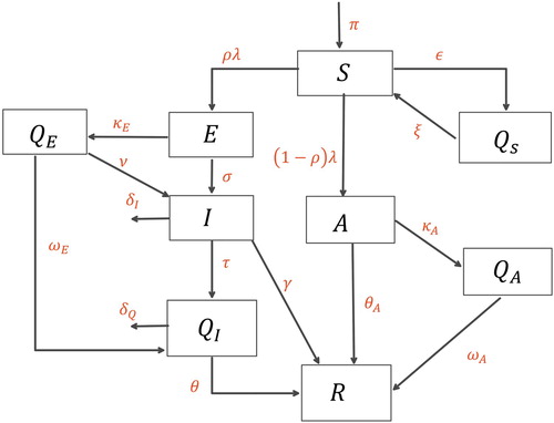
Table 1. Description of the variables of the model.

Variable	Description
N	Total population
S	Susceptible individuals
E	Individuals exposed to corona virus
$Q_S$	Individuals self quarantined
I	Individuals infected with corona virus
A	Asymptomatic individuals
$Q_E$	Quarantine of exposed individuals
$Q_I$	Isolated individuals
$Q_A$	Quarantine of asymptomatic individuals
R	Recovered from corona virus

Table 2. Description of the parameters of the model.

Parameters	Description	Values
Π	Recruitment rate of humans	100	Assumed
μ	Natural death rate of humans	60 years	Assumed
${\delta }_I$	Disease-induced death rate individuals	$0.065{\mathrm{day}}^{-1}$	Estimated
${\delta }_Q$	Disease-induced death rate of isolated individuals	$0.04{\mathrm{day}}^{-1}$	Assumed
ν	Rate of infectious of exposed quarantined individuals	0.4	Assumed
$\frac{1}{\sigma }$	Incubation rate of susceptible individuals	3−5 days	[7,8]
$\frac{1}{\gamma }$	Recovery rate of infected individuals	10 days	[7,8]
β	Effective contact rate	0.4−0.9	[7]
ρ	Probability of getting exposed to covid-19	$40\mathrm{\%}=0.4$	[7]
τ	Isolation rate of infected individuals	0.2	[7]
${\kappa }_E$	Quarantine rate of exposed individuals	0.4	Assumed
${\kappa }_A$	Quarantine rate of asymptomatic individuals	0.4	Assumed
${\omega }_E$	Isolation rate of exposed quarantined individuals	0.1	Assumed
${\omega }_A$	Recovery rate of exposed asymptomatic individuals	0.1	[7,8]
${\theta }_A$	Recovery rate of asymptomatic individuals	0.1	[7,8]
θ	Recovery rate of isolated individuals	0.05	[7,8]
ε	Self quarantine rate of susceptible individuals	0.5	Assumed
ξ	Waning rate of self quarantined individuals	0.4	Assumed
	to susceptible class
${\eta }_1$	Modification parameter for relative infectiousness	0.2	Assumed
	of isolated individuals
${\eta }_2$	Modification parameter for relative infectiousness	0.5	[7]
	of asymptomatic individuals
${\eta }_3$	Modification parameter for relative infectiousness	0.2	Assumed
	asymptomatic quarantined

3. Basic properties

The described variables in model (2(2) $\begin{array}{rl}\frac{\mathrm{d}S}{\mathrm{d}t}& =\mathrm{\Pi }+\xi Q_S-(\lambda +\mu +ϵ)S\\ \frac{\mathrm{d}{Q}_S}{\mathrm{d}t}& =ϵS-(\xi +\mu )Q_S\\ \frac{\mathrm{d}E}{\mathrm{d}t}& =\rho \lambda S-({\kappa }_E+\sigma +\mu )E\\ \frac{\mathrm{d}{Q}_E}{\mathrm{d}t}& ={\kappa }_{E}E-({\omega }_E+\nu +\mu )Q_E\\ \frac{\mathrm{d}I}{\mathrm{d}t}& =\sigma E+\nu Q_E-({\delta }_I+\tau +\mu +\gamma )I\\ \frac{\mathrm{d}A}{\mathrm{d}t}& =(1-\rho )\lambda S-({\kappa }_A+{\theta }_A+\mu )A\\ \frac{\mathrm{d}{Q}_A}{\mathrm{d}t}& ={\kappa }_{A}A-({\omega }_A+\mu )Q_A\\ \frac{\mathrm{d}{Q}_I}{\mathrm{d}t}& =\tau I+{\omega }_E{Q}_E-(\theta +{\delta }_Q+\mu )Q_I\\ \frac{\mathrm{d}R}{\mathrm{d}t}& =\theta Q_I+\gamma I+{\theta }_{A}A+{\omega }_A{Q}_A-\mu R\end{array}$(2) ) exhibit non-negative solutions for all time $t\ge 0$, i.e. the time series Solutions of model (2(2) $\begin{array}{rl}\frac{\mathrm{d}S}{\mathrm{d}t}& =\mathrm{\Pi }+\xi Q_S-(\lambda +\mu +ϵ)S\\ \frac{\mathrm{d}{Q}_S}{\mathrm{d}t}& =ϵS-(\xi +\mu )Q_S\\ \frac{\mathrm{d}E}{\mathrm{d}t}& =\rho \lambda S-({\kappa }_E+\sigma +\mu )E\\ \frac{\mathrm{d}{Q}_E}{\mathrm{d}t}& ={\kappa }_{E}E-({\omega }_E+\nu +\mu )Q_E\\ \frac{\mathrm{d}I}{\mathrm{d}t}& =\sigma E+\nu Q_E-({\delta }_I+\tau +\mu +\gamma )I\\ \frac{\mathrm{d}A}{\mathrm{d}t}& =(1-\rho )\lambda S-({\kappa }_A+{\theta }_A+\mu )A\\ \frac{\mathrm{d}{Q}_A}{\mathrm{d}t}& ={\kappa }_{A}A-({\omega }_A+\mu )Q_A\\ \frac{\mathrm{d}{Q}_I}{\mathrm{d}t}& =\tau I+{\omega }_E{Q}_E-(\theta +{\delta }_Q+\mu )Q_I\\ \frac{\mathrm{d}R}{\mathrm{d}t}& =\theta Q_I+\gamma I+{\theta }_{A}A+{\omega }_A{Q}_A-\mu R\end{array}$(2) ) for non-negative initial conditions are positive for all time $t\ge 0$.

Lemma 3.1

For any given non-negative initial conditions, there exists a unique solution $S,Q_S,E,Q_E,I,A,Q_A,Q_I,R$, respectively, for all $t\ge 0$ Moreover $\underset{t\to \mathrm{\infty }}{lim sup}N(t)\le \frac{\mathrm{\Pi }}{\mu }$

Proof is presented in the Appendix.

Lemma 3.2

The closed set: $\begin{array}{rl}\mathcal{A}& =\{\phantom{\frac{\mathrm{\Pi }}{\mu }}(S,Q_S,E,Q_E,I,A,Q_A,Q_I,R)\in R_{+}^9:S+Q_S+E+Q_E+I\\ & +A+Q_A+Q_I+R\le \frac{\mathrm{\Pi }}{\mu }\}\end{array}$ is positively invariant.

Proof is attached in the Appendix.

4. Steady state analysis

4.1. Disease-free equilibrium

The model (2(2) $\begin{array}{rl}\frac{\mathrm{d}S}{\mathrm{d}t}& =\mathrm{\Pi }+\xi Q_S-(\lambda +\mu +ϵ)S\\ \frac{\mathrm{d}{Q}_S}{\mathrm{d}t}& =ϵS-(\xi +\mu )Q_S\\ \frac{\mathrm{d}E}{\mathrm{d}t}& =\rho \lambda S-({\kappa }_E+\sigma +\mu )E\\ \frac{\mathrm{d}{Q}_E}{\mathrm{d}t}& ={\kappa }_{E}E-({\omega }_E+\nu +\mu )Q_E\\ \frac{\mathrm{d}I}{\mathrm{d}t}& =\sigma E+\nu Q_E-({\delta }_I+\tau +\mu +\gamma )I\\ \frac{\mathrm{d}A}{\mathrm{d}t}& =(1-\rho )\lambda S-({\kappa }_A+{\theta }_A+\mu )A\\ \frac{\mathrm{d}{Q}_A}{\mathrm{d}t}& ={\kappa }_{A}A-({\omega }_A+\mu )Q_A\\ \frac{\mathrm{d}{Q}_I}{\mathrm{d}t}& =\tau I+{\omega }_E{Q}_E-(\theta +{\delta }_Q+\mu )Q_I\\ \frac{\mathrm{d}R}{\mathrm{d}t}& =\theta Q_I+\gamma I+{\theta }_{A}A+{\omega }_A{Q}_A-\mu R\end{array}$(2) ) achieves a Disease-Free Equilibrium (DFE) when there is no infection induced by the disease. i.e. $\lambda =0$. Mathematically this is found by equating the right-hand side of (2(2) $\begin{array}{rl}\frac{\mathrm{d}S}{\mathrm{d}t}& =\mathrm{\Pi }+\xi Q_S-(\lambda +\mu +ϵ)S\\ \frac{\mathrm{d}{Q}_S}{\mathrm{d}t}& =ϵS-(\xi +\mu )Q_S\\ \frac{\mathrm{d}E}{\mathrm{d}t}& =\rho \lambda S-({\kappa }_E+\sigma +\mu )E\\ \frac{\mathrm{d}{Q}_E}{\mathrm{d}t}& ={\kappa }_{E}E-({\omega }_E+\nu +\mu )Q_E\\ \frac{\mathrm{d}I}{\mathrm{d}t}& =\sigma E+\nu Q_E-({\delta }_I+\tau +\mu +\gamma )I\\ \frac{\mathrm{d}A}{\mathrm{d}t}& =(1-\rho )\lambda S-({\kappa }_A+{\theta }_A+\mu )A\\ \frac{\mathrm{d}{Q}_A}{\mathrm{d}t}& ={\kappa }_{A}A-({\omega }_A+\mu )Q_A\\ \frac{\mathrm{d}{Q}_I}{\mathrm{d}t}& =\tau I+{\omega }_E{Q}_E-(\theta +{\delta }_Q+\mu )Q_I\\ \frac{\mathrm{d}R}{\mathrm{d}t}& =\theta Q_I+\gamma I+{\theta }_{A}A+{\omega }_A{Q}_A-\mu R\end{array}$(2) ) to zero. Let ${\mathcal{E}}_0$ represent the DFE of the model. $\begin{array}{rl}{\mathcal{E}}_0=& (S^{\ast },Q_S^{\ast },E^{\ast },Q_E^{\ast },I^{\ast },A^{\ast },Q_A^{\ast },Q_I^{\ast },R^{\ast })\\ {\mathcal{E}}_0=& (\frac{\pi (\mu +\xi )}{\mu (\mu +\xi +ϵ)},\frac{\pi ϵ}{\mu (\mu +\xi +ϵ)},0,0,0,0,0,0,0)\end{array}$ The local stability of the steady state ${\mathcal{E}}_0$ can be found by computing the ${\mathcal{R}}_0$ through next generation operator method [22]. The associated F and V matrices of above model (2(2) $\begin{array}{rl}\frac{\mathrm{d}S}{\mathrm{d}t}& =\mathrm{\Pi }+\xi Q_S-(\lambda +\mu +ϵ)S\\ \frac{\mathrm{d}{Q}_S}{\mathrm{d}t}& =ϵS-(\xi +\mu )Q_S\\ \frac{\mathrm{d}E}{\mathrm{d}t}& =\rho \lambda S-({\kappa }_E+\sigma +\mu )E\\ \frac{\mathrm{d}{Q}_E}{\mathrm{d}t}& ={\kappa }_{E}E-({\omega }_E+\nu +\mu )Q_E\\ \frac{\mathrm{d}I}{\mathrm{d}t}& =\sigma E+\nu Q_E-({\delta }_I+\tau +\mu +\gamma )I\\ \frac{\mathrm{d}A}{\mathrm{d}t}& =(1-\rho )\lambda S-({\kappa }_A+{\theta }_A+\mu )A\\ \frac{\mathrm{d}{Q}_A}{\mathrm{d}t}& ={\kappa }_{A}A-({\omega }_A+\mu )Q_A\\ \frac{\mathrm{d}{Q}_I}{\mathrm{d}t}& =\tau I+{\omega }_E{Q}_E-(\theta +{\delta }_Q+\mu )Q_I\\ \frac{\mathrm{d}R}{\mathrm{d}t}& =\theta Q_I+\gamma I+{\theta }_{A}A+{\omega }_A{Q}_A-\mu R\end{array}$(2) ) are given as $\begin{array}{rl}F& =\left(\begin{array}{cccccc}0& 0& \frac{\beta \rho S^{\ast }}{N^{\ast }}& \frac{\beta \rho {\eta }_2{S}^{\ast }}{N^{\ast }}& \frac{\beta \rho {\eta }_3{S}^{\ast }}{N^{\ast }}& \frac{\beta \rho {\eta }_1{S}^{\ast }}{N^{\ast }}\\ 0& 0& 0& 0& 0& 0\\ 0& 0& 0& 0& 0& 0\\ 0& 0& \frac{\beta (1-\rho )S^{\ast }}{N^{\ast }}& \frac{\beta (1-\rho ){\eta }_2{S}^{\ast }}{N^{\ast }}& \frac{\beta (1-\rho ){\eta }_3{S}^{\ast }}{N^{\ast }}& \frac{\beta (1-\rho ){\eta }_1{S}^{\ast }}{N^{\ast }}\\ 0& 0& 0& 0& 0& 0\\ 0& 0& 0& 0& 0& 0\end{array}\right)\\ V& =\left(\begin{array}{cccccc}{k}_1& 0& 0& 0& 0& 0\\ -{\kappa }_e& k_2& 0& 0& 0& 0\\ -\sigma & -\nu & k_3& 0& 0& 0\\ 0& 0& 0& k_4& 0& 0\\ 0& 0& 0& -{\kappa }_A& k_5& 0\\ 0& -{\omega }_e& -\tau & 0& 0& k_6\end{array}\right)\end{array}$ where $k_1={\kappa }_E+\sigma +\mu$, $k_2={\omega }_E+\nu +\mu$, $k_3={\delta }_I+\tau +\gamma +\mu$, $k_4={\kappa }_A+{\theta }_A+\mu$, $k_5={\omega }_A+\mu$, $k_6=\theta +{\delta }_Q+\mu$

4.2. The basic reproduction number ${\mathcal{R}}_0$

The basic reproduction number ${\mathcal{R}}_0$ is defined to be the expected number of secondary infections caused by a single infected in a fully susceptible population. Its is calculated by finding the spectral radius ρ of the matrix $F{V}^{-1}$ [22]. (4) $\begin{array}{rl}{\mathcal{R}}_0& =\frac{\beta (\mu +\xi )}{\mu +\xi +ϵ}\{\frac{(1-\rho )}{k_4}(\frac{{\eta }_3{\kappa }_A}{k_5}+{\eta }_2)\\ & +\rho [\frac{{\kappa }_e}{k_1{k}_2{k}_6}({\eta }_1{\omega }_e+\frac{\nu ({\eta }_1\tau +k_6)}{k_3})+\frac{\sigma }{k_1{k}_3}(\frac{{\eta }_1\tau }{k_6}+1)]\}\end{array}$(4)

Stability of DFE

Lemma 4.1

The steady state ${\mathcal{E}}_0$ of the model (2(2) $\begin{array}{rl}\frac{\mathrm{d}S}{\mathrm{d}t}& =\mathrm{\Pi }+\xi Q_S-(\lambda +\mu +ϵ)S\\ \frac{\mathrm{d}{Q}_S}{\mathrm{d}t}& =ϵS-(\xi +\mu )Q_S\\ \frac{\mathrm{d}E}{\mathrm{d}t}& =\rho \lambda S-({\kappa }_E+\sigma +\mu )E\\ \frac{\mathrm{d}{Q}_E}{\mathrm{d}t}& ={\kappa }_{E}E-({\omega }_E+\nu +\mu )Q_E\\ \frac{\mathrm{d}I}{\mathrm{d}t}& =\sigma E+\nu Q_E-({\delta }_I+\tau +\mu +\gamma )I\\ \frac{\mathrm{d}A}{\mathrm{d}t}& =(1-\rho )\lambda S-({\kappa }_A+{\theta }_A+\mu )A\\ \frac{\mathrm{d}{Q}_A}{\mathrm{d}t}& ={\kappa }_{A}A-({\omega }_A+\mu )Q_A\\ \frac{\mathrm{d}{Q}_I}{\mathrm{d}t}& =\tau I+{\omega }_E{Q}_E-(\theta +{\delta }_Q+\mu )Q_I\\ \frac{\mathrm{d}R}{\mathrm{d}t}& =\theta Q_I+\gamma I+{\theta }_{A}A+{\omega }_A{Q}_A-\mu R\end{array}$(2) ) is locally-asymptotically stable if ${\mathcal{R}}_0<1,$ and unstable if ${\mathcal{R}}_0>1$.

The basic implication of this theorem is that small number of the infected individuals will not lead to the large outbreaks and disease will die out in long run. To certify that the disease extinction is independent of the initially available sub-populations in model (2(2) $\begin{array}{rl}\frac{\mathrm{d}S}{\mathrm{d}t}& =\mathrm{\Pi }+\xi Q_S-(\lambda +\mu +ϵ)S\\ \frac{\mathrm{d}{Q}_S}{\mathrm{d}t}& =ϵS-(\xi +\mu )Q_S\\ \frac{\mathrm{d}E}{\mathrm{d}t}& =\rho \lambda S-({\kappa }_E+\sigma +\mu )E\\ \frac{\mathrm{d}{Q}_E}{\mathrm{d}t}& ={\kappa }_{E}E-({\omega }_E+\nu +\mu )Q_E\\ \frac{\mathrm{d}I}{\mathrm{d}t}& =\sigma E+\nu Q_E-({\delta }_I+\tau +\mu +\gamma )I\\ \frac{\mathrm{d}A}{\mathrm{d}t}& =(1-\rho )\lambda S-({\kappa }_A+{\theta }_A+\mu )A\\ \frac{\mathrm{d}{Q}_A}{\mathrm{d}t}& ={\kappa }_{A}A-({\omega }_A+\mu )Q_A\\ \frac{\mathrm{d}{Q}_I}{\mathrm{d}t}& =\tau I+{\omega }_E{Q}_E-(\theta +{\delta }_Q+\mu )Q_I\\ \frac{\mathrm{d}R}{\mathrm{d}t}& =\theta Q_I+\gamma I+{\theta }_{A}A+{\omega }_A{Q}_A-\mu R\end{array}$(2) ), it is essential to show that DFE is globally asymptotically stable (GAS).

Lemma 4.2

The Steady state ${\mathcal{E}}_0$ of model is globally asymptotically stable if ${\mathcal{R}}_0<1$ and unstable ${\mathcal{R}}_0<1$

Proof is accessible in the Appendix.

4.3. Endemic equilibrium

The endemic equilibrium is the steady state of the system (2(2) $\begin{array}{rl}\frac{\mathrm{d}S}{\mathrm{d}t}& =\mathrm{\Pi }+\xi Q_S-(\lambda +\mu +ϵ)S\\ \frac{\mathrm{d}{Q}_S}{\mathrm{d}t}& =ϵS-(\xi +\mu )Q_S\\ \frac{\mathrm{d}E}{\mathrm{d}t}& =\rho \lambda S-({\kappa }_E+\sigma +\mu )E\\ \frac{\mathrm{d}{Q}_E}{\mathrm{d}t}& ={\kappa }_{E}E-({\omega }_E+\nu +\mu )Q_E\\ \frac{\mathrm{d}I}{\mathrm{d}t}& =\sigma E+\nu Q_E-({\delta }_I+\tau +\mu +\gamma )I\\ \frac{\mathrm{d}A}{\mathrm{d}t}& =(1-\rho )\lambda S-({\kappa }_A+{\theta }_A+\mu )A\\ \frac{\mathrm{d}{Q}_A}{\mathrm{d}t}& ={\kappa }_{A}A-({\omega }_A+\mu )Q_A\\ \frac{\mathrm{d}{Q}_I}{\mathrm{d}t}& =\tau I+{\omega }_E{Q}_E-(\theta +{\delta }_Q+\mu )Q_I\\ \frac{\mathrm{d}R}{\mathrm{d}t}& =\theta Q_I+\gamma I+{\theta }_{A}A+{\omega }_A{Q}_A-\mu R\end{array}$(2) ) in the presence of the infection i.e. $\lambda \ne 0$.

Let ${\mathcal{E}}_1$ denote the arbitrary endemic equilibrium of the model (2(2) $\begin{array}{rl}\frac{\mathrm{d}S}{\mathrm{d}t}& =\mathrm{\Pi }+\xi Q_S-(\lambda +\mu +ϵ)S\\ \frac{\mathrm{d}{Q}_S}{\mathrm{d}t}& =ϵS-(\xi +\mu )Q_S\\ \frac{\mathrm{d}E}{\mathrm{d}t}& =\rho \lambda S-({\kappa }_E+\sigma +\mu )E\\ \frac{\mathrm{d}{Q}_E}{\mathrm{d}t}& ={\kappa }_{E}E-({\omega }_E+\nu +\mu )Q_E\\ \frac{\mathrm{d}I}{\mathrm{d}t}& =\sigma E+\nu Q_E-({\delta }_I+\tau +\mu +\gamma )I\\ \frac{\mathrm{d}A}{\mathrm{d}t}& =(1-\rho )\lambda S-({\kappa }_A+{\theta }_A+\mu )A\\ \frac{\mathrm{d}{Q}_A}{\mathrm{d}t}& ={\kappa }_{A}A-({\omega }_A+\mu )Q_A\\ \frac{\mathrm{d}{Q}_I}{\mathrm{d}t}& =\tau I+{\omega }_E{Q}_E-(\theta +{\delta }_Q+\mu )Q_I\\ \frac{\mathrm{d}R}{\mathrm{d}t}& =\theta Q_I+\gamma I+{\theta }_{A}A+{\omega }_A{Q}_A-\mu R\end{array}$(2) ). (5) ${\mathcal{E}}_1=(S^{\ast \ast },Q_S^{\ast \ast },E^{\ast \ast },Q_E^{\ast \ast },I^{\ast \ast },A^{\ast \ast },Q_A^{\ast \ast },Q_I^{\ast \ast },R^{\ast \ast })$(5) Moreover, Let the force of infection can be updated as ${\lambda }^{\ast \ast }=\frac{\beta }{N^{\ast \ast }}(I^{\ast \ast }+{\eta }_1{Q}_I^{\ast \ast }+{\eta }_2{A}^{\ast \ast }+{\eta }_3{Q}_A^{\ast \ast })$ with $N^{\ast \ast }=S^{\ast \ast }+Q_S^{\ast \ast }+E^{\ast \ast }+Q_E^{\ast \ast }+I^{\ast \ast }+A^{\ast \ast }+Q_A^{\ast \ast }+Q_I^{\ast \ast }+R^{\ast \ast }$ Simplifying the system (2(2) $\begin{array}{rl}\frac{\mathrm{d}S}{\mathrm{d}t}& =\mathrm{\Pi }+\xi Q_S-(\lambda +\mu +ϵ)S\\ \frac{\mathrm{d}{Q}_S}{\mathrm{d}t}& =ϵS-(\xi +\mu )Q_S\\ \frac{\mathrm{d}E}{\mathrm{d}t}& =\rho \lambda S-({\kappa }_E+\sigma +\mu )E\\ \frac{\mathrm{d}{Q}_E}{\mathrm{d}t}& ={\kappa }_{E}E-({\omega }_E+\nu +\mu )Q_E\\ \frac{\mathrm{d}I}{\mathrm{d}t}& =\sigma E+\nu Q_E-({\delta }_I+\tau +\mu +\gamma )I\\ \frac{\mathrm{d}A}{\mathrm{d}t}& =(1-\rho )\lambda S-({\kappa }_A+{\theta }_A+\mu )A\\ \frac{\mathrm{d}{Q}_A}{\mathrm{d}t}& ={\kappa }_{A}A-({\omega }_A+\mu )Q_A\\ \frac{\mathrm{d}{Q}_I}{\mathrm{d}t}& =\tau I+{\omega }_E{Q}_E-(\theta +{\delta }_Q+\mu )Q_I\\ \frac{\mathrm{d}R}{\mathrm{d}t}& =\theta Q_I+\gamma I+{\theta }_{A}A+{\omega }_A{Q}_A-\mu R\end{array}$(2) ) at this particular fix point, the endemic equilibrium becomes (6) $\begin{array}{rl}{S}^{\ast \ast }& =\frac{\pi (\mu +\xi )}{(({\lambda }^{\ast \ast }+\mu )(\mu +\xi )+\mu ϵ)};Q_S^{\ast \ast }=\frac{\pi ϵ}{({\lambda }^{\ast \ast }+\mu )(\mu +\xi )+\mu ϵ};\\ E^{\ast \ast }& =\frac{\pi {\lambda }^{\ast \ast }\rho (\mu +\xi )}{k_1(({\lambda }^{\ast \ast }+\mu )(\mu +\xi )+\mu ϵ)};\\ Q_E^{\ast \ast }& =\frac{\pi {\lambda }^{\ast \ast }\rho {\theta }_e(\mu +\xi )}{k_1{k}_2(({\lambda }^{\ast \ast }+\mu )(\mu +\xi )+\mu ϵ)}\\ I^{\ast \ast }& =\frac{\pi {\lambda }^{\ast \ast }\rho (\mu +\xi )(\nu {\theta }_e+k_2\sigma )}{k_1{k}_2{k}_3(({\lambda }^{\ast \ast }+\mu )(\mu +\xi )+\mu ϵ)};\\ A^{\ast \ast }& =\frac{\pi {\lambda }^{\ast \ast }(1-\rho )(\mu +\xi )}{k_4(({\lambda }^{\ast \ast }+\mu )(\mu +\xi )+\mu ϵ)};\\ Q_A^{\ast \ast }& =\frac{\pi {\lambda }^{\ast \ast }(1-\rho ){\kappa }_a(\mu +\xi )}{k_4{k}_5(({\lambda }^{\ast \ast }+\mu )(\mu +\xi )+\mu ϵ)};\\ Q_I^{\ast \ast }& =\frac{\pi {\lambda }^{\ast \ast }\rho (\mu +\xi )({\theta }_e(k_3{\omega }_e+\nu \tau )+k_2\sigma \tau )}{k_1{k}_2{k}_3{k}_6(({\lambda }^{\ast \ast }+\mu )(\mu +\xi )+\mu ϵ)};\\ R^{\ast \ast }& =\frac{A^{\ast \ast }{\theta }_A+\omega Q_A^{\ast \ast }+\theta Q_I^{\ast \ast }+\gamma I^{\ast \ast }}{\mu };\end{array}$(6)

Lemma 4.3

The model (2(2) $\begin{array}{rl}\frac{\mathrm{d}S}{\mathrm{d}t}& =\mathrm{\Pi }+\xi Q_S-(\lambda +\mu +ϵ)S\\ \frac{\mathrm{d}{Q}_S}{\mathrm{d}t}& =ϵS-(\xi +\mu )Q_S\\ \frac{\mathrm{d}E}{\mathrm{d}t}& =\rho \lambda S-({\kappa }_E+\sigma +\mu )E\\ \frac{\mathrm{d}{Q}_E}{\mathrm{d}t}& ={\kappa }_{E}E-({\omega }_E+\nu +\mu )Q_E\\ \frac{\mathrm{d}I}{\mathrm{d}t}& =\sigma E+\nu Q_E-({\delta }_I+\tau +\mu +\gamma )I\\ \frac{\mathrm{d}A}{\mathrm{d}t}& =(1-\rho )\lambda S-({\kappa }_A+{\theta }_A+\mu )A\\ \frac{\mathrm{d}{Q}_A}{\mathrm{d}t}& ={\kappa }_{A}A-({\omega }_A+\mu )Q_A\\ \frac{\mathrm{d}{Q}_I}{\mathrm{d}t}& =\tau I+{\omega }_E{Q}_E-(\theta +{\delta }_Q+\mu )Q_I\\ \frac{\mathrm{d}R}{\mathrm{d}t}& =\theta Q_I+\gamma I+{\theta }_{A}A+{\omega }_A{Q}_A-\mu R\end{array}$(2) ) attains the unique positive endemic equilibrium whenever ${\mathcal{R}}_0>1$.

5. Numerical simulations

The Numerical simulation are carried out with help of the ODE-45 Matlab tool. The parameters values are assumed to reflect the real pandemic. The average deaths by the corona virus is reported to be 3% [25].The parameters are summarized in the Table 2

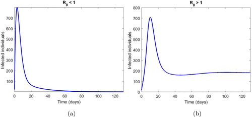
It is evident from Figure 2 that the model (2(2) $\begin{array}{rl}\frac{\mathrm{d}S}{\mathrm{d}t}& =\mathrm{\Pi }+\xi Q_S-(\lambda +\mu +ϵ)S\\ \frac{\mathrm{d}{Q}_S}{\mathrm{d}t}& =ϵS-(\xi +\mu )Q_S\\ \frac{\mathrm{d}E}{\mathrm{d}t}& =\rho \lambda S-({\kappa }_E+\sigma +\mu )E\\ \frac{\mathrm{d}{Q}_E}{\mathrm{d}t}& ={\kappa }_{E}E-({\omega }_E+\nu +\mu )Q_E\\ \frac{\mathrm{d}I}{\mathrm{d}t}& =\sigma E+\nu Q_E-({\delta }_I+\tau +\mu +\gamma )I\\ \frac{\mathrm{d}A}{\mathrm{d}t}& =(1-\rho )\lambda S-({\kappa }_A+{\theta }_A+\mu )A\\ \frac{\mathrm{d}{Q}_A}{\mathrm{d}t}& ={\kappa }_{A}A-({\omega }_A+\mu )Q_A\\ \frac{\mathrm{d}{Q}_I}{\mathrm{d}t}& =\tau I+{\omega }_E{Q}_E-(\theta +{\delta }_Q+\mu )Q_I\\ \frac{\mathrm{d}R}{\mathrm{d}t}& =\theta Q_I+\gamma I+{\theta }_{A}A+{\omega }_A{Q}_A-\mu R\end{array}$(2) ) attains the DFE and Endemic equilibrium when ${\mathcal{R}}_0$ is less than 1 and more than 1, respectively, validating our theoretical results of Lemmas.

Figure 2. Time Series Analysis. (a) ${\mathcal{R}}_0<1$. (b) ${\mathcal{R}}_0>1$.

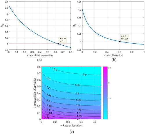
In Figure 3 we study the variation in ${\mathcal{R}}_0$ as isolation and quarantine rates are varied. We note that for realistic and particular isolation rate we need a high quarantine rate in order to keep ${\mathcal{R}}_0<1$ across a range of realistic contact rates $\beta$. We can also see this effect in the contour plot as we study the effect on ${\mathcal{R}}_0$ as both the parameters are varied. This provides support to the lock down and strict quarantine measures now in force in most countries to control the outbreak.

Figure 3. Contour graph of the self quarantine with rate of isolation and rate of isolation. (a) ε vs ${\mathcal{R}}_0$. (b) τ vs ${\mathcal{R}}_0$. (c) τ vs ε with $\beta =0.9$.

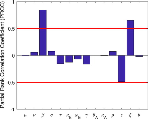
6. Sensitivity and uncertainty analysis

To be able to suggest the most efficient way of controlling the disease we need to determine the parameters we can control and to which ${\mathcal{R}}_0$ is most sensitive. Knowing this will also inform us about the parameters that need to be estimated accurately in estimating ${\mathcal{R}}_0$ from data. PRCC is an efficient sensitivity analysis method based on sampling. PRCC assigns a value between $-1$ to $+1$ for each parameter. Monotonic relationship is measured between two variables in a reliable manner by eliminating the effects (linear) of all parameters excluding the one of interest [17]. Positive PRCC value indicates a positive correlation of the parameter with the disease maintenance, whereas a negative value indicates a negative correlation with the infectiousness of the disease. The parameters studied are: $\mu ,\nu ,\beta ,\sigma ,\tau ,{\kappa }_E,{\omega }_E,\gamma ,{\theta }_A,{\kappa }_A,\rho ,ϵ,\xi ,\theta .$

From our analysis we determine that ${\mathcal{R}}_0$ is most sensitive to β, ε and τ. This points to the effectiveness of quarantine and isolation in controlling the epidemic. In the next section we consider the optimal quarantine and isolation strategies.

Uncertainty analysis enables us to quantify a degree of confidence on the model parameters by constructing a confidence interval containing 95% of the future estimates when the same assumptions are made and the only noise source is observational error. We use the Latin-hypercube sampling-based method to quantify the uncertainty of $R_0$ as a function of the model parameters. We sample independently each of the parameter distributions, and these samples are then randomly permuted forming the input parameter vectors. These samples are then used to calculate the distribution for values of ${\mathcal{R}}_0$ (Figure 4)

Figure 4. Sensitivity of the parameters.

The uncertainty analysis, as shown in Figure 5 yields an estimated value of $R_0=1.74$ with 95% CI $(2.12,1.36)$.

Figure 5. Uncertainty analysis. (a) Uncertainty of parameters, (b) Uncertainty of R₀.

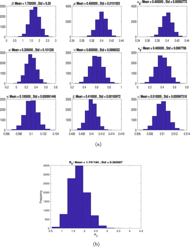
Figure 6. Optimal control of τ. (a) Cost comparison fro τ. (b) Infected pop comparison. (c) Control strategies for τ.

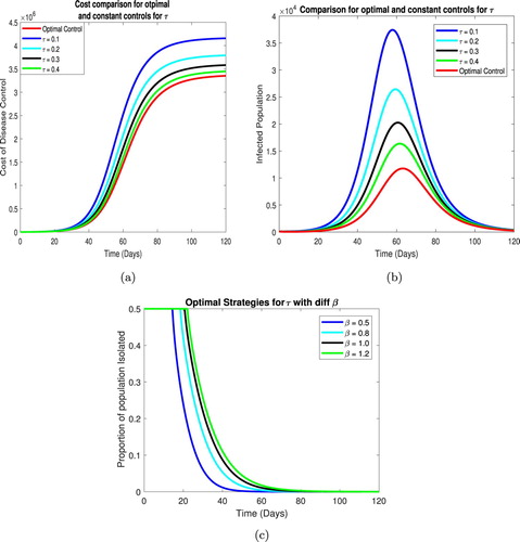
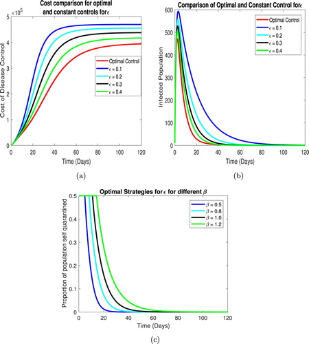
Figure 7. Optimal control for ε. (a) Cost comparison for ε. (b) Infected pop comparison. (c)Control Strategies for ε.

7. Optimal control

Optimal Control Theory uses Pontryagin's principle to reduce cost by finding optimal strategies for control parameters of the system.

Using this principle we affix an adjoint system of differential equations (with terminal conditions) to the state system to evaluate the optimal control strategy for the state system. State system along with the adjoint system is known as the optimality system. The action of the adjoint system is similar to Lagrange multiplier in a sense that it attaches constraint parameters to the state system in order to minimize maximize the functional. Further details regarding Optimal Control and adjoint system can be found in [13,21].

This paper uses optimal control theory to find quarantine (for susceptible and exposed) and isolation strategies that would minimize the total infected population and while using optimum resources. The numerical simulations were performed in MATLAB using fourth-order forward Runge–Kutta method to solve the state system and fourth-order backward Runge–Kutta method to solve the adjoint system (because of the transversality condition). The controls were updated and convergence criteria were applied similar to what M. Imran et al. did in [12].

7.1. Optimal quarantine and isolation using state system

COVID-19 is a pandemic at the moment and no vaccine or cure is available. Being highly contagious, it has spread across the globe within months. The death toll is rising and the infectious population is increasing at an alarming rate. The only ray of hope is to stop the disease from spreading by enforcing social distancing rules strictly. We study the optimal social distancing rules in this paper to be applied and for how long should they be kept in place for the disease to die out. For this purpose we define our control set U to be $U=\{\tau (t),ϵ:0\le \tau (t),ϵ\le {\gamma }_i,0\le t\le T,0<{\gamma }_i\le 1,i=1,2\}$ The Lebesgue measurable quantities $\tau ,ϵ$ are bounded above by ${\gamma }_i$, which depends on the amount of resources available for the implementation of the control strategies. The primary objective of this section is to minimize the cost functional $J[\tau (t),ϵ(t)]={\int }_0^T(I(t)+A(t)+\frac{1}{2}{W}_1{\tau }^2(t)+\frac{1}{2}{W}_2{ϵ}^2(t))\mathrm{d}t$ The $W_i$ for i = 1, 2 are cost balancing coefficients associated with the isolation, susceptible quarantine and exposed quarantine parameters. Our objective is to find the optimal values for the control parameters ${\tau }^{\ast }(t),{ϵ}^{\ast }(t)$ such that $\begin{array}{rl}J[{\tau }^{\ast }(t),{ϵ}^{\ast }(t)]& =\underset{(\tau ,ϵ)\in U}{min}J[\tau (t),ϵ(t)]\\ H& =\frac{1}{2}{W}_1{\tau }^2+\frac{1}{2}{W}_2{ϵ}^2+I+A+{\varphi }_1(\mathrm{\Pi }+\xi Q_S-(\lambda +\mu +ϵ)S)\\ & +{\varphi }_2(ϵS-(\mu +\xi )Q_S)+{\varphi }_3(\rho \lambda S-({\kappa }_e+\mu +\sigma )E)\\ & +{\varphi }_4({\kappa }_{E}E-({\omega }_E+\mu +\nu )Q_E)+{\varphi }_5(\nu Q_E+\sigma E-(\gamma +{\delta }_I+\mu +\tau )I)\\ & +{\varphi }_6((1-\rho )\lambda S-({\theta }_A+{\kappa }_A+\mu )A)+{\varphi }_7({\kappa }_{A}A-({\omega }_A+\mu )Q_A)\\ & +{\varphi }_8({\omega }_E{Q}_E+\tau I-({\delta }_A+\theta +\mu )Q_I)\\ & +{\varphi }_9({\theta }_{A}A+{\omega }_A{Q}_A+\theta Q_I+\gamma I-\mu R)\end{array}$

Theorem 7.1

There exist unique optimal controls ${\tau }^{\ast }(t),{ϵ}^{\ast }(t)$ which minimize J over U. Also, there exist an adjoint system of ${\varphi }_i^{\prime }s$ such that the optimal quarantine (susceptible) and isolation is characterized as: (7) $\begin{array}{rl}{\tau }^{\ast }(t)& =min[{\gamma }_1,max(0,\frac{I({\varphi }_5-{\varphi }_8)}{W_1})]\end{array}$(7) (8) $\begin{array}{rl}{ϵ}^{\ast }(t)& =min[{\gamma }_2,max(0,\frac{S({\varphi }_1-{\varphi }_2)}{W_2})]\end{array}$(8) The adjoint system is given as $\begin{array}{rl}\frac{\mathrm{d}{\varphi }_1}{\mathrm{d}t}& =(\mu +ϵ+\lambda ){\varphi }_1-ϵ{\varphi }_2-\rho \lambda {\varphi }_3-(1-\rho )\lambda {\varphi }_6\\ \frac{\mathrm{d}{\varphi }_2}{\mathrm{d}t}& =(\mu +\xi ){\varphi }_2-\xi {\varphi }_1\\ \frac{\mathrm{d}{\varphi }_3}{\mathrm{d}t}& =(\mu +\sigma +{\kappa }_E){\varphi }_3-{\kappa }_E{\varphi }_4-\sigma {\varphi }_5\\ \frac{\mathrm{d}{\varphi }_4}{\mathrm{d}t}& =(\mu +\nu +{\omega }_E){\varphi }_4-\nu {\varphi }_5-{\omega }_E{\varphi }_8\\ \frac{\mathrm{d}{\varphi }_5}{\mathrm{d}t}& =-1+\frac{\beta S{\varphi }_1}{N}-\frac{\beta \rho S{\varphi }_3}{N}+(\mu +\gamma +\tau +{\delta }_I){\varphi }_5-\frac{\beta (1-\rho )S{\varphi }_6}{N}-\tau {\varphi }_8-\gamma {\varphi }_9\\ \frac{\mathrm{d}{\varphi }_6}{\mathrm{d}t}& =-1+\frac{{\eta }_1\beta S{\varphi }_1}{N}-\frac{{\eta }_1\beta \rho S{\varphi }_3}{N}+(\mu +{\theta }_A+{\kappa }_A){\varphi }_6\\ & -\frac{{\eta }_1\beta (1-\rho )S{\varphi }_6}{N}-{\kappa }_A{\varphi }_7-{\theta }_A{\varphi }_9\\ \frac{\mathrm{d}{\varphi }_7}{\mathrm{d}t}& =\frac{{\eta }_2\beta S{\varphi }_1}{N}-\frac{{\eta }_2\beta \rho S{\varphi }_3}{N}-\frac{{\eta }_2\beta (1-\rho )S{\varphi }_6}{N}+(\mu +{\omega }_A){\varphi }_7-{\omega }_A{\varphi }_9\\ \frac{\mathrm{d}{\varphi }_8}{\mathrm{d}t}& =\frac{{\eta }_3\beta S{\varphi }_1}{N}-\frac{{\eta }_3\beta \rho S{\varphi }_3}{N}-\frac{{\eta }_3\beta (1-\rho )S{\varphi }_6}{N}+(\mu +\theta +{\delta }_Q){\varphi }_8-\theta {\varphi }_9\\ \frac{\mathrm{d}{\varphi }_9}{\mathrm{d}t}& =\mu {\varphi }_9\end{array}$ The above adjoint system satisfies the transversality conditions (9) $\{{\varphi }_i(T)=0,i=1,2,\dots ,9\}$(9)

7.2. Optimal control comparisons and strategies

In this section we compare the results of optimal and constant control. We first compare the cost of infection i.e. J for both strategies and then compare the infected population. Finally, we discuss the optimal strategies for the control parameters.

The optimal control cost for each parameter is less then the constant control at all times. It can be observed that for ε the cost reduction is significant compared to the other parameters which is due to the high sensitivity of parameter ε over the system.

Now we compare the total infected population using optimal and constant controls. We note a the optimal time dependent quarantine strategy, ε, yields a significant drop in infected population when compared to its constant counterparts, similarly using the optimal time dependent isolation strategy τ we see a significant drop in the infected population as compared to constant rates of isolation over time. The overall decreased population is consistent with all optimal strategies.

The optimal strategies for each parameter is evaluated for different values of the contact rate β. As β increases, so does the time for which the maximum control should be applied. For both quarantine an isolation the maximum possible quarantine and isolation rates should be maintained to the first few weeks of the disease which can then be reduced over time as depicted in Figures 6 and 7.

8. Estimation of basic reproduction number ${\mathcal{R}}_0$

The estimation of basic reproduction number ${\mathcal{R}}_0$ is based upon the estimation of the parameters that define ${\mathcal{R}}_0$. It has been carried out using nonlinear least-square method by fitting the data of COVID-19 outbreak from the Hubei province in China. We use a simplified SEIR model (10(10) $\begin{array}{rl}\frac{\mathrm{d}S}{\mathrm{d}t}& =\mathrm{\Pi }-(\frac{\beta \left(I\right)}{N}+\mu )S\\ \frac{\mathrm{d}E}{\mathrm{d}t}& =\frac{\beta \left(I\right)}{N}S-(\sigma +\mu )E\\ \frac{\mathrm{d}I}{\mathrm{d}t}& =\sigma E-(\gamma +\mu +\delta )I\\ \frac{\mathrm{d}R}{\mathrm{d}t}& =\gamma I-\mu R\end{array}$(10) ) to get this estimate. The data is sourced from 2019 Novel Corona virus COVID-19 (2019-nCoV) Data Repository by Johns Hopkins CSSE [5]. It consists of confirmed cases reported with the number of deaths and recovered people on a particular day ranging from 22 January 2020 to 13 April 2020. On a particular day, the number of infected individuals is found by subtracting the deaths and recovered people from the confirmed cases on that day. Figure 8 represents the sourced data. (10) $\begin{array}{rl}\frac{\mathrm{d}S}{\mathrm{d}t}& =\mathrm{\Pi }-(\frac{\beta \left(I\right)}{N}+\mu )S\\ \frac{\mathrm{d}E}{\mathrm{d}t}& =\frac{\beta \left(I\right)}{N}S-(\sigma +\mu )E\\ \frac{\mathrm{d}I}{\mathrm{d}t}& =\sigma E-(\gamma +\mu +\delta )I\\ \frac{\mathrm{d}R}{\mathrm{d}t}& =\gamma I-\mu R\end{array}$(10) The recruitment rate Π depends upon the demographic region from where data is collected and μ is the average natural death rate of humans.

Figure 8. Reported data and parameter estimation.

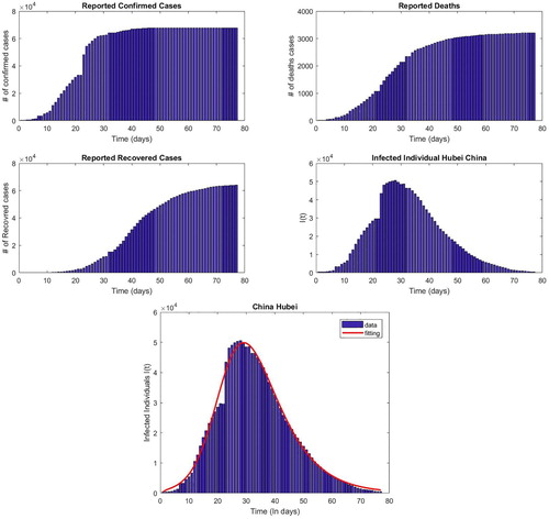
The Effective contact rate β is the critical parameter we need in order to estimate ${\mathcal{R}}_0$. It describes the rate at which susceptible and infected individuals interact with each other and the associated chance of getting infected after this interaction. It is difficult to determine this parameter directly; however, an indirect methodology proposed by Cintrón-Arias et al. [4] is used to estimate this parameter for estimating ${\mathcal{R}}_0$. (11) ${\mathcal{R}}_0=\frac{\beta \sigma }{(\mu +\sigma )(\gamma +\delta +\mu )}$(11) Calculation of ${\mathcal{R}}_0$ is carried by estimating the parameters involved using the ordinary least squares (OLS) scheme. Here we have assumed that the observed data have constant variance error distribution. Since the observed data is assumed to have constant variance error distribution. $Y_i=f(t_i,{\mathrm{\Theta }}_{\mathrm{OLS}})+{ϵ}_i$ where $Y_i$ and ${\mathrm{\Theta }}_{OLS}$ are observed values and set of parameters involving fitting model, respectively. we can estimate ${\hat{\mathrm{\Theta }}}_{OLS}$ using least squares (12) ${\hat{\mathrm{\Theta }}}_{OLS}={\arg \min }_{\mathrm{\Theta }\in \mathrm{\Omega }}\sum _{i=1}^n{[Y_i-f(t_i,\mathrm{\Theta })]}^2$(12) The numerical simulations are performed using the lsqcurvefit function from the optimization tool in Matlab. This function uses the trust-region-reflective algorithm to minimize the squared residuals.Also the bootstrap technique [6] is used to find the associated confidence intervals.

Table 3. $R_0$ Estimates.

Parameter	Estimated values	$95\mathrm{\%}$ CI
β	1.248	1.2−1.3
γ	0.603	0.59−0.63
σ	0.546	0.52−0.57
δ	0.065	0.0047−0.1
${\mathcal{R}}_0$	1.8678	1.36−2.4

9. Conclusions

In this study we presented a compartmental ordinary differential equation model to understand the transmission dynamics of COVID-19. We incorporated the role of asymptomatic individuals as well as effects of quarantine and isolation of different population groups. We analysed the model to suggest strategies for effective control of the epidemic. We also estimated $R_0$ for the Wuhan outbreak.

After establishing the existence of a threshold quantity $R_0$ such that the outbreak dies out if $R_0<1$ and the disease is endemic if $R_0>1$, we look at the model parameters to which $R_0$ is most sensitive. These turn out to be the contact rate (as expected) and the quarantine (ε) and isolation (τ) rates. We study the variation of $R_0$ with these parameters, our analysis shows that we need a high rate of quarantine along with isolation of infected individuals in order to control the disease. This lends support to the lock down measures adopted across the globe to help combat the outbreak.

Using optimal control methods we suggest quarantine and isolation strategies. The study shows that at the early stages of the outbreak we need the maximum possible levels of quarantine and isolation, with these rates dropping over time, the reduction depending on the contact rate. Further, our analysis reveals that an optimal control rather than a high constant control is preferable. This means that quarantining and isolating according the proposed strategy (as opposed to a high constant control) has a more favourable impact in controlling the disease while keeping the costs.

In the last section we use a simplified model to estimate $R_0$ for the outbreak in Wuhan. Using the disease incidence data we use a simple least square fit, the estimated value comes out to be $R_0=1.87$. The value is within range of various estimates in the literature, it is towards the lower side as we have used a simplified model and the effects of the strict quarantine and isolation measures by the Wuhan authorities are reflected in a lower contacted rate on which we base our estimate of $R_0$. A follow up study using more elaborate models to estimate $R_0$ is being done and we will report further findings in the future.

The pandemic is still ongoing and in many countries the epidemic cure is yet to 'turn'. Our study is an attempt to use mathematical models to provide health authorities some insights into the disease dynamics to help them in decision making for effective disease control.

Disclosure statement

No potential conflict of interest was reported by the author(s).

Appendix

A.1. Proof of Lemma 3.1

Proof.

Adding the right-hand side of model (2(2) $\begin{array}{rl}\frac{\mathrm{d}S}{\mathrm{d}t}& =\mathrm{\Pi }+\xi Q_S-(\lambda +\mu +ϵ)S\\ \frac{\mathrm{d}{Q}_S}{\mathrm{d}t}& =ϵS-(\xi +\mu )Q_S\\ \frac{\mathrm{d}E}{\mathrm{d}t}& =\rho \lambda S-({\kappa }_E+\sigma +\mu )E\\ \frac{\mathrm{d}{Q}_E}{\mathrm{d}t}& ={\kappa }_{E}E-({\omega }_E+\nu +\mu )Q_E\\ \frac{\mathrm{d}I}{\mathrm{d}t}& =\sigma E+\nu Q_E-({\delta }_I+\tau +\mu +\gamma )I\\ \frac{\mathrm{d}A}{\mathrm{d}t}& =(1-\rho )\lambda S-({\kappa }_A+{\theta }_A+\mu )A\\ \frac{\mathrm{d}{Q}_A}{\mathrm{d}t}& ={\kappa }_{A}A-({\omega }_A+\mu )Q_A\\ \frac{\mathrm{d}{Q}_I}{\mathrm{d}t}& =\tau I+{\omega }_E{Q}_E-(\theta +{\delta }_Q+\mu )Q_I\\ \frac{\mathrm{d}R}{\mathrm{d}t}& =\theta Q_I+\gamma I+{\theta }_{A}A+{\omega }_A{Q}_A-\mu R\end{array}$(2) ) results in total (A1) $\begin{array}{rl}\frac{\mathrm{d}N}{\mathrm{d}t}& =\mathrm{\Pi }-\mu N-({\delta }_I+{\delta }_Q)\le \mathrm{\Pi }-\mu N\\ \frac{\mathrm{d}N}{\mathrm{d}t}& \le \mathrm{\Pi }-\mu N\end{array}$(A1) It follows that (A2) $N(t)\le N(0){\mathrm{e}}^{-\mu t}+\frac{\pi }{\mu }(1-e^{-\mu t})$(A2) Therefore solutions exists, and are eventually bounded on every finite time interval.

A.2. Proof of Lemma 3.2

Proof.

From (A1(A1) $\begin{array}{rl}\frac{\mathrm{d}N}{\mathrm{d}t}& =\mathrm{\Pi }-\mu N-({\delta }_I+{\delta }_Q)\le \mathrm{\Pi }-\mu N\\ \frac{\mathrm{d}N}{\mathrm{d}t}& \le \mathrm{\Pi }-\mu N\end{array}$(A1) ) and (A2(A2) $N(t)\le N(0){\mathrm{e}}^{-\mu t}+\frac{\pi }{\mu }(1-e^{-\mu t})$(A2) ), it follows that as time approaches to infinity $t\to \mathrm{\infty }$ $N(t)\le \frac{\mathrm{\Pi }}{\mu }$ Hence, the set $\mathcal{A}$ is positively invariant.

A.3. Proof of Lemma 4.2

Proof.

Using comparison theorem, we can construct the equations of the model (2(2) $\begin{array}{rl}\frac{\mathrm{d}S}{\mathrm{d}t}& =\mathrm{\Pi }+\xi Q_S-(\lambda +\mu +ϵ)S\\ \frac{\mathrm{d}{Q}_S}{\mathrm{d}t}& =ϵS-(\xi +\mu )Q_S\\ \frac{\mathrm{d}E}{\mathrm{d}t}& =\rho \lambda S-({\kappa }_E+\sigma +\mu )E\\ \frac{\mathrm{d}{Q}_E}{\mathrm{d}t}& ={\kappa }_{E}E-({\omega }_E+\nu +\mu )Q_E\\ \frac{\mathrm{d}I}{\mathrm{d}t}& =\sigma E+\nu Q_E-({\delta }_I+\tau +\mu +\gamma )I\\ \frac{\mathrm{d}A}{\mathrm{d}t}& =(1-\rho )\lambda S-({\kappa }_A+{\theta }_A+\mu )A\\ \frac{\mathrm{d}{Q}_A}{\mathrm{d}t}& ={\kappa }_{A}A-({\omega }_A+\mu )Q_A\\ \frac{\mathrm{d}{Q}_I}{\mathrm{d}t}& =\tau I+{\omega }_E{Q}_E-(\theta +{\delta }_Q+\mu )Q_I\\ \frac{\mathrm{d}R}{\mathrm{d}t}& =\theta Q_I+\gamma I+{\theta }_{A}A+{\omega }_A{Q}_A-\mu R\end{array}$(2) ) infected compartments as (A3) $\begin{array}{rl}{\left(\begin{array}{c}E\\ Q_E\\ I\\ A\\ Q_A\\ Q_I\end{array}\right)}^{\prime }& =\mathrm{\Omega }\left(\frac{S}{N}\right)F\left(\begin{array}{c}E\\ Q_E\\ I\\ A\\ Q_A\\ Q_I\end{array}\right)-V\left(\begin{array}{c}E\\ Q_E\\ I\\ A\\ Q_A\\ Q_I\end{array}\right)-\mathrm{\Omega }F\left(\begin{array}{c}E\\ Q_E\\ I\\ A\\ Q_A\\ Q_I\end{array}\right)-\left(\begin{array}{c}1\\ 0\\ 0\\ 1\\ 0\\ 0\end{array}\right)\\ {\left(\begin{array}{c}E\\ Q_E\\ I\\ A\\ Q_A\\ Q_I\end{array}\right)}^{\prime }& \le \mathrm{\Omega }\left(\frac{S}{N}\right)F\left(\begin{array}{c}E\\ Q_E\\ I\\ A\\ Q_A\\ Q_I\end{array}\right)-V\left(\begin{array}{c}E\\ Q_E\\ I\\ A\\ Q_A\\ Q_I\end{array}\right)-\mathrm{\Omega }F\left(\begin{array}{c}E\\ Q_E\\ I\\ A\\ Q_A\\ Q_I\end{array}\right)\\ {\left(\begin{array}{c}E\\ Q_E\\ I\\ A\\ Q_A\\ Q_I\end{array}\right)}^{\prime }& \le (F-V)\left(\begin{array}{c}E\\ Q_E\\ I\\ A\\ Q_A\\ Q_I\end{array}\right)\end{array}$(A3) where $\mathrm{\Omega }=\frac{N^{\ast }}{S^{\ast }}$.

Since Lemma 4.1 guaranties that ${\mathcal{E}}_0$ is locally asymptotically stable when ${\mathcal{R}}_0<1$ or, Equivalently saying that all eigenvalues of F−V matrix have negative real parts [22]. Hence the inequality system (A3(A3) $\begin{array}{rl}{\left(\begin{array}{c}E\\ Q_E\\ I\\ A\\ Q_A\\ Q_I\end{array}\right)}^{\prime }& =\mathrm{\Omega }\left(\frac{S}{N}\right)F\left(\begin{array}{c}E\\ Q_E\\ I\\ A\\ Q_A\\ Q_I\end{array}\right)-V\left(\begin{array}{c}E\\ Q_E\\ I\\ A\\ Q_A\\ Q_I\end{array}\right)-\mathrm{\Omega }F\left(\begin{array}{c}E\\ Q_E\\ I\\ A\\ Q_A\\ Q_I\end{array}\right)-\left(\begin{array}{c}1\\ 0\\ 0\\ 1\\ 0\\ 0\end{array}\right)\\ {\left(\begin{array}{c}E\\ Q_E\\ I\\ A\\ Q_A\\ Q_I\end{array}\right)}^{\prime }& \le \mathrm{\Omega }\left(\frac{S}{N}\right)F\left(\begin{array}{c}E\\ Q_E\\ I\\ A\\ Q_A\\ Q_I\end{array}\right)-V\left(\begin{array}{c}E\\ Q_E\\ I\\ A\\ Q_A\\ Q_I\end{array}\right)-\mathrm{\Omega }F\left(\begin{array}{c}E\\ Q_E\\ I\\ A\\ Q_A\\ Q_I\end{array}\right)\\ {\left(\begin{array}{c}E\\ Q_E\\ I\\ A\\ Q_A\\ Q_I\end{array}\right)}^{\prime }& \le (F-V)\left(\begin{array}{c}E\\ Q_E\\ I\\ A\\ Q_A\\ Q_I\end{array}\right)\end{array}$(A3) ) is stable whenever ${\mathcal{R}}_0<1$. So by comparison theorem, all compartments $E,Q_E,I,A,Q_A,Q_I$ approaches to 0 as $t\to \mathrm{\infty }$ Therefore substituting these values to model (2(2) $\begin{array}{rl}\frac{\mathrm{d}S}{\mathrm{d}t}& =\mathrm{\Pi }+\xi Q_S-(\lambda +\mu +ϵ)S\\ \frac{\mathrm{d}{Q}_S}{\mathrm{d}t}& =ϵS-(\xi +\mu )Q_S\\ \frac{\mathrm{d}E}{\mathrm{d}t}& =\rho \lambda S-({\kappa }_E+\sigma +\mu )E\\ \frac{\mathrm{d}{Q}_E}{\mathrm{d}t}& ={\kappa }_{E}E-({\omega }_E+\nu +\mu )Q_E\\ \frac{\mathrm{d}I}{\mathrm{d}t}& =\sigma E+\nu Q_E-({\delta }_I+\tau +\mu +\gamma )I\\ \frac{\mathrm{d}A}{\mathrm{d}t}& =(1-\rho )\lambda S-({\kappa }_A+{\theta }_A+\mu )A\\ \frac{\mathrm{d}{Q}_A}{\mathrm{d}t}& ={\kappa }_{A}A-({\omega }_A+\mu )Q_A\\ \frac{\mathrm{d}{Q}_I}{\mathrm{d}t}& =\tau I+{\omega }_E{Q}_E-(\theta +{\delta }_Q+\mu )Q_I\\ \frac{\mathrm{d}R}{\mathrm{d}t}& =\theta Q_I+\gamma I+{\theta }_{A}A+{\omega }_A{Q}_A-\mu R\end{array}$(2) ) results in $S\to S^{\ast }$, $Q_S\to Q_S^{\ast }$ and $R\to 0$. Thus attaining the ${\mathcal{E}}_0$ for ${\mathcal{R}}_0<1$. Hence the steady state ${\mathcal{E}}_0$ is globally asymptotically stable GAS.

A.4. Proof of Theorem 7.1

Proof.

The proof follows similar steps in [12]. The integrand of our functional J is convex with respect to $\tau (t),ϵ(t)$. Our solution for the model is bounded above by $N(t)\le (\mathrm{\Pi }/\mu )$ for all t. The model has Lipschitz property with regard to the state variables. The convex property of integrand of the functional J with respect to the set U ensures a unique optimal control, based on the boundedness of the state solutions, and the Lipschitz property of the state system with respect to the state variables [9]. Hence the existence of optimal control is established.

The adjoint system is obtained through the following evaluations: $\begin{array}{rl}\frac{\mathrm{d}{\varphi }_1}{\mathrm{d}t}& =-\frac{\mathrm{\partial }{H}^{\ast }}{\mathrm{\partial }S},{\varphi }_1(T)=0\\ \frac{\mathrm{d}{\varphi }_2}{\mathrm{d}t}& =-\frac{\mathrm{\partial }{H}^{\ast }}{\mathrm{\partial }{Q}_S},{\varphi }_2(T)=0\\ ⋮\\ \frac{\mathrm{d}{\varphi }_9}{\mathrm{d}t}& =-\frac{\mathrm{\partial }{H}^{\ast }}{\mathrm{\partial }R},{\varphi }_9(T)=0\end{array}$ The optimality condition gives: $\begin{array}{rl}\frac{\mathrm{\partial }{H}^{\ast }}{\mathrm{\partial }\tau }& =0⟹\tau =(\frac{I({\varphi }_5-{\varphi }_8)}{W_1})\\ \frac{\mathrm{\partial }{H}^{\ast }}{\mathrm{\partial }ϵ}& =0⟹ϵ=(\frac{S({\varphi }_1-{\varphi }_2)}{W_2})\end{array}$ Since $\tau ,ϵ$ are bounded in U by ${\tau }_{max}\mathrm{and}{ϵ}_{max}$, respectively, optimal control becomes: $\begin{array}{rl}{\tau }^{\ast }(t)& =min[{\tau }_{max},max(0,\frac{I({\varphi }_5-{\varphi }_8)}{W_1})]\\ {ϵ}^{\ast }(t)& =min[{ϵ}_{max},max(0,\frac{S({\varphi }_1-{\varphi }_2)}{W_2})]\end{array}$ The uniqueness of optimality system implies the uniqueness of optimal control.

References

- H.I. Aslan, M. Demir, M.M. Wise, and S. Lenhart, Modeling COVID-19: Forecasting and analyzing the dynamics of the outbreak in Hubei and Turkey, preprint. doi:10.1101/2020.04.11.20061952.
- Centers for Disease Control and Prevention, Coronavirus disease 2019 (COVID-19), 2020. Available at https://www.cdc.gov/coronavirus/2019-ncov/ (accessed 25 April 2020).
- T. Chen, J. Rui, Q. Wang, Z. Zhao, J. Cui, and L. Yin, A mathematical model for simulating the phase-based transmissibility of a novel coronavirus, Infect. Dis. Poverty 9(1) (2020). doi:10.1186/s40249-020-00640-3.
- A. Cintrón-Arias, C. Castillo-Cháivez, L.M.A. Bettencourt, A.L. Lloyd, and H.T. Banks, The estimation of the effective reproductive number from disease outbreak data, Math. Biosci. Eng. 6 (2009), pp. 261–282. doi:10.3934/mbe.2009.6.261.
- Data.humdata.org, Novel Coronavirus (COVID-19) Cases Data – Humanitarian Data Exchange, 2020. Available at https://data.humdata.org/dataset/novel-coronavirus-2019-ncov-cases (accessed 7 April 2020).
- B. Efron and R.J. Tibshirani, An Introduction to the Bootstrap, Chapman & Hall/CRC, Boca Raton, FL, 1993.
- S. Eikenberry, M. Mancuso, E. Iboi, T. Phan, K. Eikenberry, Y. Kuang, E. Kostelich, and A. Gumel, To mask or not to mask: Modeling the potential for face mask use by the general public to curtail the COVID-19 pandemic, Infect. Dis. Model. 5 (2020), pp. 293–308.
- N. Ferguson, D. Laydon, G. Nedjati Gilani, N. Imai, K. Ainslie, M. Baguelin, S. Bhatia, A. Boonyasiri, Z. Cucunuba Perez, G. Cuomo-Dannenburg, A. Dighe, I. Dorigatti, H. Fu, K. Gaythorpe, W. Green, A. Hamlet, W. Hinsley, L. Okell, S. Van Elsland, H. Thompson, R. Verity, E. Volz, H. Wang, Y.Wang, P. Walker, C. Walters, P. Winskill, C. Whittaker, C. Donnelly, S. Riley, and A. Ghani, Report 9: Impact of non-pharmaceutical interventions (Npis) to reduce COVID19 mortality and healthcare demand, 2020. [online] Hdl.handle.net. Available at http://hdl.handle.net/10044/1/77482 (accessed 2 May 2020).
- W. Fleming and R. Rishel, Deterministic and Stochastic Optimal Control, Springer-Verlag, Berlin, 1975.
- B. Hu, X. Fi, L. Fa, Bat Origin of human coronaviruses. Virol J 12, 221 (2015). https://doi.org/10.1186/s12985-015-0422-1.
- C. Huang, Y. Wang, X. Li, and L. Ren, Clinical features of patients infected with 2019 novel coronavirus in Wuhan, China Lancet 395 (2020), pp. 497–506. doi: 10.1016/S0140-6736(20)30183-5
- M. Imran, A. Khan, A. Ansari, and S. Shah, Modeling transmission dynamics of Ebola virus disease, Int. J. Biomath. 10(04) (2017), p. 1750057. doi: 10.1142/S1793524517500577
- D. Kirschner, S. Lenhart, and S. Serbin, Optimal control of the chemotherapy of HIV, J. Math. Biol.35(7) (1997), pp. 775–792. doi: 10.1007/s002850050076
- A.J. Kucharski, T.W. Russell, C. Diamond, Y. Liu, J. Edmunds, S. Funk, R.M. Eggo, F. Sun, M. Jit, J.D. Munday, and N. Davies, Early dynamics of transmission and control of COVID-19: A mathematical modelling study, Lancet Infect. Dis. 20 (2020), pp. 30144–4. doi:10.1016/s1473-3099. doi: 10.1016/S1473-3099(20)30144-4
- Q. Lin, S. Zhao, D. Gao, Y. Lou, S. Yang, S.S. Musa, M.H. Wang, Y. Cai, W. Wang, L. Yang, and D. He, A conceptual model for the coronavirus disease 2019 (COVID-19) outbreak in Wuhan, China with individual reaction and governmental action, Int. J. Infect. Dis. 93 (2020), pp. 211–216. doi:10.1016/j.ijid.2020.02.058.
- S. Mandal, T. Bhatnagar, N. Arinaminpathy, A. Agarwal, A. Chowdhury, M. Murhekar, R.R.Gangakhedkar, and S. Sarkar, Prudent public health intervention strategies to control the coronavirus disease 2019 transmission in India: A mathematical model-based approach, Indian J. Med. Res. 151(2) (2020), pp. 190–199. doi:10.4103/ijmr.ijmr_504_20.
- S. Marino, I.B. Hogue, C.J. Ray, and D.E. Kirschner, A methodology for performing global uncertainty and sensitivity analysis in systems biology, J. Theor. Biol 254 (2008), pp. 178–196. doi:10.1016/j.jtbi.2008.04.011.
- Oie.int., Questions and answers on the COVID-19: OIE – world organisation for animal health, 2020. Available at https://www.oie.int/scientific-expertise/specific-information-and-recommendations/questions-and-answers-on-2019novel-coronavirus (accessed 25 April 2020).
- L. Pang, S. Liu, X. Zhang, Transission dynamics and control strategies of COVID-19 in Wihan China. J. Biol. Syst. XX (2020), pp. 1–18. doi: 10.1142/S0218339020500096
- A. Perkins and G. Espana, Optimal control of the COVID-19 pandemic with non-pharmaceutical interventions, preprint. doi:10.1101/2020.04.22.20076018.
- L.S. Pontryagin, V.G. Boltyanskii, The Mathematical Theory of Optimal Processes, John Wiley & Sons New York/London1962.
- P. van den Driessche and J. Watmough, Reproduction numbers and sub-threshold endemic equilibria for compartmental models of disease transmission, Math. Biosci. 180 (2002), pp. 29–48. doi: 10.1016/S0025-5564(02)00108-6
- Who.int., Coronavirus, 2020. Available at https://www.who.int/health-topics/coronavirus (accessed 25 April 2020).
- Worldometers. info., Coronavirus update (Live): 2,874,022 cases and 200,790 deaths from COVID-19 virus pandemic – worldometer, 2020. Available at https://www.worldometers.info/coronavirus/ (accessed 25 April 2020).
- Worldometers.info., Coronavirus mortality rate (COVID-19) – worldometer, 2020. Available at https://www.worldometers.info/coronavirus/coronavirus-death-rate/#who-03-03-20 (accessed 19 April 2020).
- J. Yang, Y. Zheng, X. Gou, K. Pu, Z. Chen, Q. Guo, R. Ji, H. Wang, Y. Wang, and Y. Zhou, Prevalence of comorbidities and its effects in coronavirus disease 2019 patient: A systematic review and meta-analysis, Int. J. Infect. Dis. 94 (2020), pp. 91–95. doi: 10.1016/j.ijid.2020.03.017
- S. Zhao, Q. Lin, J. Ran, S.S. Musa, G. Yang, W. Wangh, Y. Loue, D. Gao, L. Yang, D. He, and M.H.Wang, Preliminary estimation of the basic reproduction number of novel coronavirus (2019-nCoV) in China, from 2019 to 2020: A data-driven analysis in the early phase of the outbreak, Int. J. Infect. Dis.92 (2020), pp. 214–217. doi:10.1016/j.ijid.2020.01.050.