Modeling the suppression dynamics of Aedes mosquitoes with mating inhomogeneity

Abstract

A novel strategy for controlling mosquito-borne diseases, such as dengue, malaria and Zika, involves releases of Wolbachia-infected mosquitoes as Wolbachia cause early embryo death when an infected male mates with an uninfected female. In this work, we introduce a delay differential equation model with mating inhomogeneity to discuss mosquito population suppression based on Wolbachia. Our analyses show that the wild mosquitoes could be eliminated if either the adult mortality rate exceeds the threshold ${\delta }_A^{\ast }$ or the release amount exceeds the threshold $r^{\ast }$ uniformly. We also present the nonlinear dependence of ${\delta }_A^{\ast }$ and $r^{\ast }$ on the parameters, respectively, as well as the effect of pesticide spraying on wild mosquitoes. Our simulations suggest that the releasing should be started at least 5 weeks before the peak dengue season, taking into account both the release amount and the suppression speed.

Keywords:

• Dengue fever
• Wolbachia
• cytoplasmic incompatibility
• mosquito population suppression
• delay differential equation model

2010 Mathematics Subject Classifications:

• 92B05
• 37N25
• 34D23
• 92D30

1. Introduction

With the global aggressive invading of mosquitoes by urbanization, international trades and travels, mosquito-borne diseases, such as dengue, malaria and Zika have become a major public health concern. Dengue, increasing more than 30-fold globally in the past few decades, infects over 390 million people annually in the tropical and subtropical regions [4,42]. The mechanism of antibody-dependent enhancement greatly increases the difficulty of vaccine development. It was reported that 130 vaccinated children had died after using Dengvaxia, the first registered dengue vaccine [1]. Thus the key measure to prevent mosquito-borne diseases is to reduce the population of mosquito vectors. Pesticide application has already been the primary method for mosquito eradication in the world. To defeat the unprecedented dengue outbreak in Guangzhou in 2014, more than 27,000 kg pyrethroids were sprayed in over 3291 km${}^2$ of land [41]. However, pesticide spraying is not a perfect solution as it also leads to environmental pollution and insecticide resistance of mosquitoes [25,34].

An innovative technique for the control of mosquito-borne diseases involves Wolbachia, which is a genus of common intracellular bacterial endosymbionts and was first identified in 1924 [13,35]. The infection of Wolbachia can reduce host's ability to reproduce and transmit disease-causing viruses [5,39,40,43]. Due to the mechanism cytoplasmic incompatibility (CI), the insects cannot produce offspring when infected males cross with field females which are not infected with the same strain [11,27]. Thus repeated release of Wolbachia-infected males in the field could suppress the wild mosquitoes, and a preparatory work is to clarify the suppression dynamics, i.e. the dynamical changes of wild mosquito population under the intervention of infected males.

Mosquito population suppression has become a very active research topic in recent years and various mathematical models have been formulated and analysed for studying the wild mosquito population suppression effects on the releases of sterile male mosquitoes as well as Wolbachia-infected male mosquitoes, for example, difference equation models [47,51], ordinary differential equation models [7,12,50], delay differential equation models [2,6,19,20,23], and reaction-diffusion equation models [17,18,32], etc. By combining sterile insect techniques and Wolbachia, Zheng et al. have successfully eradicated more than 90% of Aedes albopictus in Shazai island in Guangzhou recently [52], which verifies the feasibility of mosquito population suppression in the field. Because in the interaction dynamics, the fundamental and only role for sterile male mosquitoes or Wolbachia-infected male mosquitoes is to mate with wild female mosquitoes, so that the mating wild female mosquitoes either fail to reproduce or lay eggs that do not hatch. The author in [44] proposed a new modelling idea of mosquito population inhibition that is completely different from the existing modelling approaches, where $R\left(t\right)$, the number of sterile male mosquitoes or Wolbachia-infected male mosquitoes released at time t, is just regarded as a given function instead of an independent variable satisfying a dynamic equation. This idea has been well developed and used recently, see for example [20–22,28,45,46]. In [45], the authors only considered those sexually active sterile mosquitoes in the model and ignored the death of those sterile mosquitoes, and clearly explained why the case when $R\left(t\right)\equiv r$, a constant, is possible, we also refer to [28]. We know that once sterile mosquitoes lose their mating competitiveness, they have no effect on the wild mosquito population suppression, even if they are still alive. In this work, we continue to follow such an idea in [44] and focus on the classical Allee effect to formulate and analyse a mosquito population suppression model with time delay. Let $A\left(t\right)$ be the size of wild adult mosquitoes, distributing equally in sex [14,15,51], and uniformly in space [17,18]. The wild mosquitoes are interfered by releasing Wolbachia-infected males with size $R\left(t\right)$ which induce complete CI to wild females [16,49]. By random mating, for a single female, the chance of incompatible mating equals to the number of infected males $R\left(t\right)$ over the total number of males $A\left(t\right)/2+R\left(t\right)$. Let τ be the average development period from oviposition to the eclosion of adults, and ${\delta }_I$ be the natural mortality rate of the immature stage. Hence the birth rate of a female adult is given by (1) $e^{-{\delta }_I\tau }\cdot \frac{A(t-\tau )/2}{A(t-\tau )/2+R(t-\tau )}\cdot \chi \left(A\right(t-\tau )/2+R(t-\tau \left)\right),$(1) where $e^{-{\delta }_I\tau }$ denotes the mean survival probability from egg to adult and $\chi (A/2+R)$ the average number of adult offsprings by a female. As the opportunity of a female to mate with a male in a small population is lower than that in a large population, we follow the idea of the classical Allee effect to describe the mating inhomogeneity [7]. Let β be the average number of larvae by a female and assume (2) $\chi (A/2+R)=\text{β}\frac{A/2+R}{\alpha +A/2+R},$(2) where α is a positive constant. We use the logistic model to describe the mortality rate of adults with natural mortality rate m, and a constraint constant K associated with density-dependent competition [19,20,44] (3) $f\left(A\right)=m\left(1+\frac{A+R}{K}\right)A.$(3) By combining (1(1) $e^{-{\delta }_I\tau }\cdot \frac{A(t-\tau )/2}{A(t-\tau )/2+R(t-\tau )}\cdot \chi \left(A\right(t-\tau )/2+R(t-\tau \left)\right),$(1) )–(3(3) $f\left(A\right)=m\left(1+\frac{A+R}{K}\right)A.$(3) ) and setting $b=\text{β}{e}^{-{\delta }_I\tau }/2$, we derive the following delay differential equation: (4) $\frac{\mathrm{d}A\left(t\right)}{\mathrm{d}t}=\frac{b{A}^2(t-\tau )}{2\alpha +A(t-\tau )+2R(t-\tau )}-m\left(1+\frac{A\left(t\right)+R\left(t\right)}{K}\right)A\left(t\right).$(4) We let $A\left(t\right)=A(t,t_0,\phi )$ denote the solution of (4(4) $\frac{\mathrm{d}A\left(t\right)}{\mathrm{d}t}=\frac{b{A}^2(t-\tau )}{2\alpha +A(t-\tau )+2R(t-\tau )}-m\left(1+\frac{A\left(t\right)+R\left(t\right)}{K}\right)A\left(t\right).$(4) ) subjecting to the initial function $\phi \in C\left(\right[t_0-\tau ,t_0],(0,\mathrm{\infty }\left)\right)$, for some $t_0\ge 0$.

Our discussions in the following parts focus on system (4(4) $\frac{\mathrm{d}A\left(t\right)}{\mathrm{d}t}=\frac{b{A}^2(t-\tau )}{2\alpha +A(t-\tau )+2R(t-\tau )}-m\left(1+\frac{A\left(t\right)+R\left(t\right)}{K}\right)A\left(t\right).$(4) ). In Section 2, we present complete descriptions of the dynamics of wild mosquitoes by delicate analyses based on the Fluctuation Lemma [36]. By setting $R\left(t\right)>0$ (or $R\left(t\right)\equiv 0$) in (4(4) $\frac{\mathrm{d}A\left(t\right)}{\mathrm{d}t}=\frac{b{A}^2(t-\tau )}{2\alpha +A(t-\tau )+2R(t-\tau )}-m\left(1+\frac{A\left(t\right)+R\left(t\right)}{K}\right)A\left(t\right).$(4) ), we obtain the dynamics of wild mosquitoes with (or without) the intervention of released infected males. The results summarized in Theorems 2.1–2.6 present sufficient conditions for the extinction of wild mosquitoes in different situations. We identify an adult mortality rate threshold ${\delta }_A^{\ast }$ and a release amount threshold $r^{\ast }$. The wild mosquitoes could be eliminated if either the adult mortality rate exceeds ${\delta }_A^{\ast }$ or the release amount exceeds $r^{\ast }$ uniformly. When the releasing number is kept constant less than $r^{\ast }$, (4(4) $\frac{\mathrm{d}A\left(t\right)}{\mathrm{d}t}=\frac{b{A}^2(t-\tau )}{2\alpha +A(t-\tau )+2R(t-\tau )}-m\left(1+\frac{A\left(t\right)+R\left(t\right)}{K}\right)A\left(t\right).$(4) ) displays a bistable dynamics with two asymptotically stable equilibria $A_0$ and $A_2$ and an unstable equilibrium $A_1$. When $R\left(t\right)\equiv r^{\ast }$, the two positive equilibria $A_1$ and $A_2$ coincide into ${\tilde{A}}_1$, which is semistable, i.e. asymptotically stable from right-side and unstable from left-side. In Section 3, by letting the parameters in (4(4) $\frac{\mathrm{d}A\left(t\right)}{\mathrm{d}t}=\frac{b{A}^2(t-\tau )}{2\alpha +A(t-\tau )+2R(t-\tau )}-m\left(1+\frac{A\left(t\right)+R\left(t\right)}{K}\right)A\left(t\right).$(4) ) be temperature-dependent on a daily basis, we use simulations to examine how the temporal profiles of wild mosquito population respond to the variation of temperature. By using the daily average temperatures from 2011 to 2017 in Guangzhou, the simulated curves capture several critical features of wild Aedes albopictus population in Guangzhou. We employ the model to design the most cost-efficient releasing policy, targeting at more than $95\mathrm{\%}$ reduction at the highest mosquito density. Our simulation shows that the releasing should be started no less than 5 weeks before the peak period of wild mosquito density.

2. Threshold dynamics of population suppression

By studying the global dynamics of (4(4) $\frac{\mathrm{d}A\left(t\right)}{\mathrm{d}t}=\frac{b{A}^2(t-\tau )}{2\alpha +A(t-\tau )+2R(t-\tau )}-m\left(1+\frac{A\left(t\right)+R\left(t\right)}{K}\right)A\left(t\right).$(4) ), we can obtain the precise expression of the releasing threshold over which the population suppression is guaranteed. For each initial function $\phi \in C\left(\right[t_0-\tau ,t_0],(0,\mathrm{\infty }\left)\right)$, the positiveness and boundedness of the solution $A\left(t\right)=A(t,t_0,\phi )$ to (4(4) $\frac{\mathrm{d}A\left(t\right)}{\mathrm{d}t}=\frac{b{A}^2(t-\tau )}{2\alpha +A(t-\tau )+2R(t-\tau )}-m\left(1+\frac{A\left(t\right)+R\left(t\right)}{K}\right)A\left(t\right).$(4) ) can be proved by a similar method in [21,22].

As $b=\text{β}{e}^{-{\delta }_I\tau }/2$ counts the fertility of adult females and m measures its natural mortality rate, it holds naturally that b>m. We assume throughout the rest of this paper that (5) $b_0=\frac{b}{m}-1>0.$(5)

2.1. A classification of the equilibria

In the case $R\left(t\right)\equiv 0$, (4(4) $\frac{\mathrm{d}A\left(t\right)}{\mathrm{d}t}=\frac{b{A}^2(t-\tau )}{2\alpha +A(t-\tau )+2R(t-\tau )}-m\left(1+\frac{A\left(t\right)+R\left(t\right)}{K}\right)A\left(t\right).$(4) ) reduces to (6) $\frac{\mathrm{d}A\left(t\right)}{\mathrm{d}t}=\frac{b{A}^2(t-\tau )}{2\alpha +A(t-\tau )}-m\left(1+\frac{A\left(t\right)}{K}\right)A\left(t\right),$(6) which characterizes the dynamics of the wild mosquito population. Obviously, $A_0=0$ is the unique constant steady-state of (4(4) $\frac{\mathrm{d}A\left(t\right)}{\mathrm{d}t}=\frac{b{A}^2(t-\tau )}{2\alpha +A(t-\tau )+2R(t-\tau )}-m\left(1+\frac{A\left(t\right)+R\left(t\right)}{K}\right)A\left(t\right).$(4) ) when the release number of infected males $R\left(t\right)$ changes in time t. If the loss of crossable infected males in the field is compensated by a new release such that $R\left(t\right)$ is maintained almost at a constant level, then it can be modelled by setting $R\left(t\right)\equiv r\ge 0$. Besides the trivial equilibrium $A_0$, we enumerate the nonnegative equilibria of (4(4) $\frac{\mathrm{d}A\left(t\right)}{\mathrm{d}t}=\frac{b{A}^2(t-\tau )}{2\alpha +A(t-\tau )+2R(t-\tau )}-m\left(1+\frac{A\left(t\right)+R\left(t\right)}{K}\right)A\left(t\right).$(4) ) in the following lemma.

Lemma 2.1

Let $b_0>0,$ $R\left(t\right)\equiv r\ge 0,$ and (7) $K^{\ast }=\frac{2\alpha }{b_0^2}(\sqrt{b_0+1}+1{)}^2,r^{\ast }=(3b_0+4)K-2\alpha -2\sqrt{2(b_0+1)\left[\right(b_0+2)K-\alpha ]K}.$(7) Then the positive equilibria of (4(4) $\frac{\mathrm{d}A\left(t\right)}{\mathrm{d}t}=\frac{b{A}^2(t-\tau )}{2\alpha +A(t-\tau )+2R(t-\tau )}-m\left(1+\frac{A\left(t\right)+R\left(t\right)}{K}\right)A\left(t\right).$(4) ) can be classified as follows:

1. For the case $K>K^{\ast },$ we have $r^{\ast }>0$ and (4(4) $\frac{\mathrm{d}A\left(t\right)}{\mathrm{d}t}=\frac{b{A}^2(t-\tau )}{2\alpha +A(t-\tau )+2R(t-\tau )}-m\left(1+\frac{A\left(t\right)+R\left(t\right)}{K}\right)A\left(t\right).$(4) ) has no positive equilibrium when $r>r^{\ast },$ a unique positive equilibrium (8) ${\tilde{A}}_1=\frac{b_{0}K-2\alpha -3r^{\ast }}{2}$(8) when $r=r^{\ast },$ two positive equilibria (9) $A_1=\frac{b_{0}K-2\alpha -3r-\sqrt{D(r,K)}}{2},A_2=\frac{b_{0}K-2\alpha -3r+\sqrt{D(r,K)}}{2}$(9) when $r<r^{\ast },$ where (10) $D(r,K)=r^2-2\left[\right(3b_0+4)K-2\alpha ]r+(b_{0}K-2\alpha {)}^2-8\alpha K.$(10) Specially, if $r=0,$ then (6(6) $\frac{\mathrm{d}A\left(t\right)}{\mathrm{d}t}=\frac{b{A}^2(t-\tau )}{2\alpha +A(t-\tau )}-m\left(1+\frac{A\left(t\right)}{K}\right)A\left(t\right),$(6) ) has two positive equilibria (11) $A_1^{\ast }=\frac{b_{0}K-2\alpha -\sqrt{F\left(K\right)}}{2},A_2^{\ast }=\frac{b_{0}K-2\alpha +\sqrt{F\left(K\right)}}{2},$(11) where $F\left(K\right)=(b_{0}K-2\alpha {)}^2-8\alpha K$.

2. For the case $K=K^{\ast },$ we have $r^{\ast }=0,$ and (4(4) $\frac{\mathrm{d}A\left(t\right)}{\mathrm{d}t}=\frac{b{A}^2(t-\tau )}{2\alpha +A(t-\tau )+2R(t-\tau )}-m\left(1+\frac{A\left(t\right)+R\left(t\right)}{K}\right)A\left(t\right).$(4) ) has no positive equilibrium when $r>0,$ a unique positive equilibrium (12) ${\tilde{A}}_2=\frac{b_0}{2}K-\alpha$(12) when r = 0.

3. For the case $K<K^{\ast }$, we have $r^{\ast }<0,$ and (4(4) $\frac{\mathrm{d}A\left(t\right)}{\mathrm{d}t}=\frac{b{A}^2(t-\tau )}{2\alpha +A(t-\tau )+2R(t-\tau )}-m\left(1+\frac{A\left(t\right)+R\left(t\right)}{K}\right)A\left(t\right).$(4) ) or (6(6) $\frac{\mathrm{d}A\left(t\right)}{\mathrm{d}t}=\frac{b{A}^2(t-\tau )}{2\alpha +A(t-\tau )}-m\left(1+\frac{A\left(t\right)}{K}\right)A\left(t\right),$(6) ) has no positive equilibrium for all $r\ge 0$.

Proof.

We only present the proof for Part (1) as the proof for the other two cases is similar. Besides $A_0$=0, a positive constant steady-state of (4(4) $\frac{\mathrm{d}A\left(t\right)}{\mathrm{d}t}=\frac{b{A}^2(t-\tau )}{2\alpha +A(t-\tau )+2R(t-\tau )}-m\left(1+\frac{A\left(t\right)+R\left(t\right)}{K}\right)A\left(t\right).$(4) ) is a positive zero of quadratic form (13) $g(x,r)=x^2-(b_{0}K-2\alpha -3r)x+2(r+\alpha )(r+K),$(13) with discriminant $D(r,K)$ defined in (10(10) $D(r,K)=r^2-2\left[\right(3b_0+4)K-2\alpha ]r+(b_{0}K-2\alpha {)}^2-8\alpha K.$(10) ). If $D(r,K)>0$, then $g(x,r)=0$ has two solutions (14) $x_1=\frac{b_{0}K-2\alpha -3r-\sqrt{D(r,K)}}{2}\mathrm{a}\mathrm{n}\mathrm{d}{x}_2=\frac{b_{0}K-2\alpha -3r+\sqrt{D(r,K)}}{2},$(14) satisfying $x_1+x_2=b_{0}K-2\alpha -3r$ and $x_1{x}_2=2(r+\alpha )(r+K)>0$. Set $K_1=2\alpha /b_0$, $r_1=(b_{0}K-2\alpha )/3.$ Then $x_2>x_1>0$ if and only if (15) $K>K_1\mathrm{a}\mathrm{n}\mathrm{d}r<r_1.$(15) As we only care about the positive solutions of $g(x,r)=0$, we assume (15(15) $K>K_1\mathrm{a}\mathrm{n}\mathrm{d}r<r_1.$(15) ) holds in this Part. The discriminant of $D(r,K)=0$ is ${△}_r=32(b_0+1)\left[\right(b_0+2)K-\alpha ]K.$ It is easy to verify that ${△}_r>0$ if and only if $K>K_2:=\alpha /(b_0+2).$ Note that $K_2=\alpha /(b_0+2)<2\alpha /b_0=K_1.$ If $K>K_1$, then $K>K_2$ and $D(r,K)=0$ has two roots $\begin{array}{rl}{r}^{\ast }& =(3b_0+4)K-2\alpha -2\sqrt{2(b_0+1)\left[\right(b_0+2)K-\alpha ]K},\\ r_2& =(3b_0+4)K-2\alpha +2\sqrt{2(b_0+1)\left[\right(b_0+2)K-\alpha ]K}.\end{array}$ Since $r^{\ast }<r_2$ and $r^{\ast }+r_2=2\left[\right(3b_0+4)K-2\alpha ]>2\left[\right(3b_0+4)K_1-2\alpha ]=4\alpha (b_0+2)/b_0>0$, we obtain $r_2>0$. To find out whether $r^{\ast }$ is greater than 0, we define (16) $F\left(K\right)=r^{\ast }{r}_2=(b_{0}K-2\alpha {)}^2-8\alpha K=b_0^2{K}^2-4\alpha (b_0+2)K+4{\alpha }^2.$(16) Then $r^{\ast }>0$ if and only if $F\left(K\right)>0$. As $F\left(K\right)=0$ has two positive zeros (17) $K_3=\frac{2\alpha }{b_0^2}{\left(\sqrt{b_0+1}-1\right)}^2\mathrm{a}\mathrm{n}\mathrm{d}{K}^{\ast }=\frac{2\alpha }{b_0^2}{\left(\sqrt{b_0+1}+1\right)}^2,$(17) we have $r^{\ast }>0$ when $K>K^{\ast }$ or $0<K<K_3$, $r^{\ast }=0$ when $K=K^{\ast }$ or $K=K_3$, and $r^{\ast }<0$ when $K_3<K<K^{\ast }$. By using $\begin{array}{r}{K}^{\ast }-K_1=\frac{2\alpha }{b_0^2}{\left(\sqrt{b_0+1}+1\right)}^2-\frac{2\alpha }{b_0}=\frac{4\alpha }{b_0^2}\left(1+\sqrt{b_0+1}\right)>0\end{array}$ and $\begin{array}{r}{K}_1-K_3=\frac{2\alpha }{b_0}-\frac{2\alpha }{b_0^2}{\left(\sqrt{b_0+1}-1\right)}^2=\frac{4\alpha }{b_0^2}\left(\sqrt{b_0+1}-1\right)>0,\end{array}$ we obtain $K_3<K_1<K^{\ast }$. Thus $r^{\ast }>0$ only when $K>K^{\ast }$.

Next we consider the relation among $r^{\ast }$, $r_1$ and $r_2$. As $K>K_1$, we have $\begin{array}{r}(2b_0+3)K-\alpha >(2b_0+3)K_1-\alpha =\frac{3\alpha (b_0+2)}{b_0}>0,\end{array}$ and so $r_2-r_1=\frac{4}{3}\left[\right(2b_0+3)K-\alpha ]+2\sqrt{2(b_0+1)\left[\right(b_0+2)K-\alpha ]K}>0.$ Since $\begin{array}{r}{r}^{\ast }-r_1=\frac{4}{3}\left[\right(2b_0+3)K-\alpha ]-2\sqrt{2(b_0+1)\left[\right(b_0+2)K-\alpha ]K},\end{array}$ we have $r^{\ast }<r_1$ if and only if $2\left[\right(2b_0+3)K-\alpha ]<3\sqrt{2(b_0+1)\left[\right(b_0+2)K-\alpha ]K},$ i.e. (18) $h\left(K\right):=b_0(b_0+3)K^2-\alpha (b_0-3)K-2{\alpha }^2>0.$(18) Note that the unique positive zero $K_4$ of $h\left(K\right)$ satisfying $K_4=2\alpha /(b_0+3)<2\alpha /b_0=K_1$. Then $K>K_1$ implies $K>K_4$ and so $h\left(K\right)>0$. Thus $r^{\ast }<r_1<r_2$. As $r<r_1$ from condition (15(15) $K>K_1\mathrm{a}\mathrm{n}\mathrm{d}r<r_1.$(15) ), we derive that $x_{1,2}>0$ only when $0\le r<r^{\ast }$. Then for the case $K>K^{\ast }$, $g(x,r)=0$ has two different positive roots when $0\le r<r^{\ast }$, a unique positive root $\tilde{x}=(b_{0}K-2\alpha -3r^{\ast })/2$ when $r=r^{\ast }$, and no positive root when $r>r_1$. The proof of Part (1) is completed.

2.2. The bistability and semistability under insufficient releasing

In this section, we discuss the suppression dynamics based on the releasing number $R\left(t\right)$ and the density-dependent competitive constant K according to Lemma 2.1. We first introduce Fluctuation Lemma which is important throughout this section.

Lemma 2.2

Fluctuation Lemma [36]: Appendix A.5

Let $f:[b,\mathrm{\infty })\to R$ be bounded and differentiable. Then there exist sequences $s_k,$ $t_k\to \mathrm{\infty }$ such that $f\left(s_k\right)\to \underset{\_}{f},f^{\prime }\left(s_k\right)\to 0,\mathrm{a}\mathrm{n}\mathrm{d}f\left(t_k\right)\to \overline{f},f^{\prime }\left(t_k\right)\to 0\mathrm{a}\mathrm{s}k\to \mathrm{\infty },$ where $\overline{f}:=\underset{t\to \mathrm{\infty }}{lim sup}f\left(t\right)$ and $\underset{\_}{f}:=\underset{t\to \mathrm{\infty }}{lim inf}f\left(t\right)$.

Now we start to discuss the stabilities of the equilibria of system (4(4) $\frac{\mathrm{d}A\left(t\right)}{\mathrm{d}t}=\frac{b{A}^2(t-\tau )}{2\alpha +A(t-\tau )+2R(t-\tau )}-m\left(1+\frac{A\left(t\right)+R\left(t\right)}{K}\right)A\left(t\right).$(4) ). We first show that the mosquito-free equilibrium $A_0$ is locally stable for small initial size when $K>K^{\ast }$.

Lemma 2.3

Let $K>K^{\ast }$, ${\overline{r}}_0=\underset{t\in [t_0-\tau ,\mathrm{\infty })}{inf}R\left(t\right)$ and $r_0=min\{{\overline{r}}_0,r^{\ast }\}$. If the initial function satisfies $\phi \left(t\right)<min\left\{A_1\right(r_0),{\tilde{A}}_1(r_0\left)\right\}$, where ${\tilde{A}}_1\left(r_0\right)$ and $A_1\left(r_0\right)$ are equilibria of (4(4) $\frac{\mathrm{d}A\left(t\right)}{\mathrm{d}t}=\frac{b{A}^2(t-\tau )}{2\alpha +A(t-\tau )+2R(t-\tau )}-m\left(1+\frac{A\left(t\right)+R\left(t\right)}{K}\right)A\left(t\right).$(4) ) defined in (8(8) ${\tilde{A}}_1=\frac{b_{0}K-2\alpha -3r^{\ast }}{2}$(8) ) and (9(9) $A_1=\frac{b_{0}K-2\alpha -3r-\sqrt{D(r,K)}}{2},A_2=\frac{b_{0}K-2\alpha -3r+\sqrt{D(r,K)}}{2}$(9) ), respectively, then the solution $A\left(t\right)$ of (4(4) $\frac{\mathrm{d}A\left(t\right)}{\mathrm{d}t}=\frac{b{A}^2(t-\tau )}{2\alpha +A(t-\tau )+2R(t-\tau )}-m\left(1+\frac{A\left(t\right)+R\left(t\right)}{K}\right)A\left(t\right).$(4) ) satisfies (19) $\underset{t\to \mathrm{\infty }}{lim}A\left(t\right)=0.$(19)

Proof.

We first prove the positivity and boundedness of the solutions of (4(4) $\frac{\mathrm{d}A\left(t\right)}{\mathrm{d}t}=\frac{b{A}^2(t-\tau )}{2\alpha +A(t-\tau )+2R(t-\tau )}-m\left(1+\frac{A\left(t\right)+R\left(t\right)}{K}\right)A\left(t\right).$(4) ). If $A\left(t\right)>0$ does not hold for all $t\ge 0$, we let $\overline{t}>t_0$ be the least time such that $A\left(\overline{t}\right)=0$. Hence $A^{\prime }\left(\overline{t}\right)\le 0$, and so $\begin{array}{r}0<\frac{b{A}^2(\overline{t}-\tau )}{2\alpha +A(\overline{t}-\tau )+2R(\overline{t}-\tau )}\le 0.\end{array}$ This contradiction verifies the positivity of $A\left(t\right)$. If $A\left(t\right)$ is an unbounded solution of (4(4) $\frac{\mathrm{d}A\left(t\right)}{\mathrm{d}t}=\frac{b{A}^2(t-\tau )}{2\alpha +A(t-\tau )+2R(t-\tau )}-m\left(1+\frac{A\left(t\right)+R\left(t\right)}{K}\right)A\left(t\right).$(4) ), then there is an increasing sequence $\left\{t_n\right\}$ with $t_n\to \mathrm{\infty }$ as $n\to \mathrm{\infty }$, such that $\left\{A\right(t_n\left)\right\}$ increases monotonically to infinity as $n\to \mathrm{\infty }$, $A(t_n-\tau )<A\left(t_n\right)$, and $A^{\prime }\left(t_n\right)\ge 0$. Thus $\begin{array}{r}m\left(1+\frac{A\left(t_n\right)+R\left(t_n\right)}{K}\right)<\frac{bA\left(t_n\right)}{2\alpha +A\left(t_n\right)+2R(\overline{t}-\tau )},\end{array}$ which is impossible for large n, and therefore all the solutions of (4(4) $\frac{\mathrm{d}A\left(t\right)}{\mathrm{d}t}=\frac{b{A}^2(t-\tau )}{2\alpha +A(t-\tau )+2R(t-\tau )}-m\left(1+\frac{A\left(t\right)+R\left(t\right)}{K}\right)A\left(t\right).$(4) ) are bounded.

The nonnegativity of $R\left(t\right)$ indicates that $r_0=\underset{t\in [t_0-\tau ,\mathrm{\infty })}{inf}R\left(t\right)\ge 0$. By Lemma 2.1, $A_1\left(r_0\right)$ and ${\tilde{A}}_1\left(r_0\right)$ are well defined and positive when $r_0<r^{\ast }$ and $r_0=r^{\ast }$, respectively. For any a with $0<a<min\left\{A_1\right(r_0),{\tilde{A}}_1(r_0\left)\right\}$, we claim that (20) $0<A\left(t\right)<a\mathrm{f}\mathrm{o}\mathrm{r}t\ge t_0\mathrm{i}\mathrm{f}0<\phi \left(t\right)<a\mathrm{o}\mathrm{n}[t_0-\tau ,t_0].$(20) If not, then there is some $\overline{t}>t_0$, such that $A\left(\overline{t}\right)=a$, and $A\left(t\right)<a$ for $t\in [t_0,\overline{t})$, then $A^{\prime }\left(\overline{t}\right)\ge 0$. Substituting $t=\overline{t}$ into (4(4) $\frac{\mathrm{d}A\left(t\right)}{\mathrm{d}t}=\frac{b{A}^2(t-\tau )}{2\alpha +A(t-\tau )+2R(t-\tau )}-m\left(1+\frac{A\left(t\right)+R\left(t\right)}{K}\right)A\left(t\right).$(4) ) leads to $\begin{array}{r}m\left(1+\frac{a+r_0}{K}\right)a\le m\left(1+\frac{a+R\left(\overline{t}\right)}{K}\right)a<\frac{b{a}^2}{2\alpha +a+2R(\overline{t}-\tau )}\le \frac{b{a}^2}{2\alpha +a+2r_0}.\end{array}$ Hence $\begin{array}{r}m\left(1+\frac{a+r_0}{K}\right)<\frac{ba}{2\alpha +a+2r_0}.\end{array}$ Setting x = a and $r=r_0$ in (13(13) $g(x,r)=x^2-(b_{0}K-2\alpha -3r)x+2(r+\alpha )(r+K),$(13) ) leads to $g(a,r_0)<0$. Note that $g(x,r_0)>0$ when $0\le x<A_1\left(r_0\right)$ for the case $r_0<r^{\ast }$, or $0\le x<{\tilde{A}}_1\left(r_0\right)$ for the case $r_0=r^{\ast }$. This contradiction guarantees (20(20) $0<A\left(t\right)<a\mathrm{f}\mathrm{o}\mathrm{r}t\ge t_0\mathrm{i}\mathrm{f}0<\phi \left(t\right)<a\mathrm{o}\mathrm{n}[t_0-\tau ,t_0].$(20) ), which verifies the locally uniform stability of $A_0$.

Assume that $0\le \phi \left(t\right)<min\left\{A_1\right(r_0),{\tilde{A}}_1(r_0\left)\right\}$ for $t\in [t_0-\tau ,t_0]$. By the claim (20(20) $0<A\left(t\right)<a\mathrm{f}\mathrm{o}\mathrm{r}t\ge t_0\mathrm{i}\mathrm{f}0<\phi \left(t\right)<a\mathrm{o}\mathrm{n}[t_0-\tau ,t_0].$(20) ), if $\phi \left(t\right)<a<min\left\{A_1\right(r_0),{\tilde{A}}_1(r_0\left)\right\}$ on $[t_0-\tau ,t_0]$, then $A\left(t\right)<a$ and so the upper limit $\overline{A}=\underset{t\to \mathrm{\infty }}{lim sup}A\left(t\right)\le a$. As the solution is bounded, there is a sequence $\left\{t_n\right\}$ such that (21) $A\left(t_n\right)\to \overline{A}=\underset{t\to \mathrm{\infty }}{lim sup}A\left(t\right),A^{\prime }\left(t_n\right)\to 0\mathrm{a}\mathrm{n}\mathrm{d}{t}_n\to \mathrm{\infty },\mathrm{a}\mathrm{s}n\to \mathrm{\infty },$(21) by Fluctuation Lemma (Lemma 2.2). Taking the limit of (4(4) $\frac{\mathrm{d}A\left(t\right)}{\mathrm{d}t}=\frac{b{A}^2(t-\tau )}{2\alpha +A(t-\tau )+2R(t-\tau )}-m\left(1+\frac{A\left(t\right)+R\left(t\right)}{K}\right)A\left(t\right).$(4) ) along this sequence gives (22) $\begin{array}{rl}m\left(1+\frac{\overline{A}+r_0}{K}\right)\overline{A}& \le m\left(1+\frac{\overline{A}+R\left(t_n\right)}{K}\right)\overline{A}\\ & =\underset{n\to \mathrm{\infty }}{lim sup}\frac{b{A}^2(t_n-\tau )}{2\alpha +A(t_n-\tau )+2R(t_n-\tau )}\\ & \le \frac{b{\overline{A}}^2}{2\alpha +\overline{A}+2R(t_n-\tau )}\\ & \le \frac{b{\overline{A}}^2}{2\alpha +\overline{A}+2r_0}.\end{array}$(22) Hence $\overline{A}=0$ or $\begin{array}{r}m\left(1+\frac{\overline{A}+r_0}{K}\right)\le \frac{b\overline{A}}{2\alpha +\overline{A}+2r_0},\end{array}$ which leads to $g(\overline{A},r_0)\le 0$. The facts $g(x,r_0)>0$ on $[0,min\{A_1\left(r_0\right),{\tilde{A}}_1\left(r_0\right)\left\}\right)$ and $0\le \overline{A}\le a<min\left\{A_1\right(r_0),{\tilde{A}}_1(r_0\left)\right\}$ indicate $g(\overline{A},0)>0$, which contradicts the second case. Thus $\overline{A}=0$. By the positivity of $A\left(t\right)$, we obtain that the lower limit of the solution $\underset{\_}{A}=\underset{t\to \mathrm{\infty }}{lim inf}A\left(t\right)\ge 0$. Hence $\underset{\_}{A}=\overline{A}=0$, which verifies the asymptotic stability of $A_0$.

When $K>K^{\ast }$ and the releasing number maintains at a constant level such that $R\left(t\right)\equiv r\in (0,r^{\ast })$, Lemma 2.1 indicates that (4(4) $\frac{\mathrm{d}A\left(t\right)}{\mathrm{d}t}=\frac{b{A}^2(t-\tau )}{2\alpha +A(t-\tau )+2R(t-\tau )}-m\left(1+\frac{A\left(t\right)+R\left(t\right)}{K}\right)A\left(t\right).$(4) ) has a mosquito-free equilibrium $A_0=0$ and two positive equilibria $A_1$ and $A_2$ defined in (9(9) $A_1=\frac{b_{0}K-2\alpha -3r-\sqrt{D(r,K)}}{2},A_2=\frac{b_{0}K-2\alpha -3r+\sqrt{D(r,K)}}{2}$(9) ). We next show that (4(4) $\frac{\mathrm{d}A\left(t\right)}{\mathrm{d}t}=\frac{b{A}^2(t-\tau )}{2\alpha +A(t-\tau )+2R(t-\tau )}-m\left(1+\frac{A\left(t\right)+R\left(t\right)}{K}\right)A\left(t\right).$(4) ) exhibits bistable dynamics with an unstable equilibrium $A_1$ being sandwiched by two asymptotically stable equilibria $A_0$ and $A_2$.

Theorem 2.1

Let $K>K^{\ast }$ and $R\left(t\right)\equiv r\in (0,r^{\ast })$ for $t\ge 0$. Let $A\left(t\right)$ be a solution of (4(4) $\frac{\mathrm{d}A\left(t\right)}{\mathrm{d}t}=\frac{b{A}^2(t-\tau )}{2\alpha +A(t-\tau )+2R(t-\tau )}-m\left(1+\frac{A\left(t\right)+R\left(t\right)}{K}\right)A\left(t\right).$(4) ). Then we have:

1. $A_1$ is unstable;

2. $\underset{t\to \mathrm{\infty }}{lim}A\left(t\right)=0$ when $\phi \left(t\right)\le A_1$ on $[t_0-\tau ,t_0]$ and $\phi \left(t\right)\not\equiv A_1;$

3. $\underset{t\to \mathrm{\infty }}{lim}A\left(t\right)=A_2$ when $\phi \left(t\right)\ge A_1$ on $[t_0-\tau ,t_0]$ and $\phi \left(t\right)\not\equiv A_1$.

Proof.

(1) The instability of $A_1$ follows from Lemma 2.3 directly.

(2) Let ${\mathcal{A}}_0\left(t\right)$ be an arbitrary solution of (4(4) $\frac{\mathrm{d}A\left(t\right)}{\mathrm{d}t}=\frac{b{A}^2(t-\tau )}{2\alpha +A(t-\tau )+2R(t-\tau )}-m\left(1+\frac{A\left(t\right)+R\left(t\right)}{K}\right)A\left(t\right).$(4) ) with $\phi \left(t\right)\le A_1$ on $[t_0-\tau ,t_0]$ and $\phi \left(t\right)\not\equiv A_1$. By setting $\phi \left(t\right)\equiv A_1$ for $t\in [t_0-\tau ,t_0]$ we obtain a constant solution ${\mathcal{A}}_1\left(t\right)\equiv A_1$. We claim that ${\mathcal{A}}_0\left(t\right)\le {\mathcal{A}}_1\left(t\right)$ for all $t\ge 0$. Let $A_{\epsilon }\left(t\right)$ be a solution of (4(4) $\frac{\mathrm{d}A\left(t\right)}{\mathrm{d}t}=\frac{b{A}^2(t-\tau )}{2\alpha +A(t-\tau )+2R(t-\tau )}-m\left(1+\frac{A\left(t\right)+R\left(t\right)}{K}\right)A\left(t\right).$(4) ) with $A_{\epsilon }\left(t\right)=A_0\left(t\right)-\epsilon$ for $t-\tau \le t\le t_0$. For sufficiently small $\epsilon >0$, it is easy to verify $A_{\epsilon }\left(t\right)<A_1\left(t\right)$ for $t\ge 0$. Thus $Li{m}_{\epsilon \to 0^{+}}{A}_{\epsilon }\left(t\right)\le A_1\left(t\right)$, implying that $A_0\left(t\right)\le A_1\left(t\right)$ for $t\ge 0$. Since $\phi \left(t\right)\not\equiv A_1$, then ${\mathcal{A}}_0\left(t\right)\not\equiv A_1$ when $t\in [t_0,t_0+\tau ]$ and we can find $t_1$ and $t_2$ such that ${\mathcal{A}}_0\left(t\right)<A_1$ when $t\in [t_1,t_2]\subseteq [t_0,t_0+\tau ]$. Let ${\mathcal{A}}_2\left(t\right)$ be a solution of (4(4) $\frac{\mathrm{d}A\left(t\right)}{\mathrm{d}t}=\frac{b{A}^2(t-\tau )}{2\alpha +A(t-\tau )+2R(t-\tau )}-m\left(1+\frac{A\left(t\right)+R\left(t\right)}{K}\right)A\left(t\right).$(4) ) with the continuous initial function $\begin{array}{rl}\overline{\phi }\left(t\right)& =A_1\mathrm{f}\mathrm{o}\mathrm{r}t\in [t_2-\tau ,t_1],{\mathcal{A}}_0\left(t\right)\le \overline{\phi }\left(t\right)\le A_1\mathrm{f}\mathrm{o}\mathrm{r}t\in (t_1,t_2),\\ \overline{\phi }\left(t_2\right)& ={\mathcal{A}}_0\left(t_2\right).\end{array}$ Since ${\mathcal{A}}_0\left(t\right)\le \overline{\phi }\left(t\right)$ when $t\in [t_2-\tau ,t_1]$, we obtain ${\mathcal{A}}_0\left(t\right)\le {\mathcal{A}}_2\left(t\right)$ when $t\in [t_2,t_1+\tau ]$ by the similar method as the proof for ${\mathcal{A}}_0\left(t\right)\le {\mathcal{A}}_1\left(t\right)$. Note that $\begin{array}{r}\frac{\mathrm{d}{\mathcal{A}}_1\left(t\right)}{\mathrm{d}t}=\frac{b{A}_1^2}{2\alpha +A_1+2r}-m\left(1+\frac{{\mathcal{A}}_1\left(t\right)+r}{K}\right){\mathcal{A}}_1\left(t\right),\\ \frac{\mathrm{d}{\mathcal{A}}_2\left(t\right)}{\mathrm{d}t}=\frac{b{A}_1^2}{2\alpha +A_1+2r}-m\left(1+\frac{{\mathcal{A}}_2\left(t\right)+r}{K}\right){\mathcal{A}}_2\left(t\right)\end{array}$ when $t\in [t_2,t_1+\tau ]$, which are two ordinary differential equations. Then by the fact ${\mathcal{A}}_2\left(t_2\right)<{\mathcal{A}}_1\left(t_2\right)$ we get ${\mathcal{A}}_2\left(t\right)<{\mathcal{A}}_1\left(t\right)$ when $t\in [t_2,t_1+\tau ]$. Thus we have ${\mathcal{A}}_0\left(t\right)\le {\mathcal{A}}_2\left(t\right)<{\mathcal{A}}_1\left(t\right)=A_1$ for $t\in [t_2,t_1+\tau ]$, then we derive $\underset{t\to \mathrm{\infty }}{lim}A\left(t\right)=0$ by Lemma 2.3.

(3) By the proof of Part (1), we only need to prove the case $\phi \left(t\right)>A_1$ on $[t_0-\tau ,t_0]$. Similar to the claim (20(20) $0<A\left(t\right)<a\mathrm{f}\mathrm{o}\mathrm{r}t\ge t_0\mathrm{i}\mathrm{f}0<\phi \left(t\right)<a\mathrm{o}\mathrm{n}[t_0-\tau ,t_0].$(20) ) in Lemma 2.3, we claim that, for any positive constant $a<A_2-A_1$, (23) $|A\left(t\right)-A_2|<a\mathrm{f}\mathrm{o}\mathrm{r}t\ge t_0\mathrm{i}\mathrm{f}|\phi \left(t\right)-A_2|<a\mathrm{o}\mathrm{n}[t_0-\tau ,t_0].$(23) If not, we let $\overline{t}>t_0$ again be the least time at which $A=A_2-a$ or $A=A_2+a$. If $A\left(\overline{t}\right)=A_2-a$, then $A\left(t\right)>A_2-a$ for $t\in [t_0,\overline{t})$ and $A^{\prime }\left(\overline{t}\right)\le 0$. From (4(4) $\frac{\mathrm{d}A\left(t\right)}{\mathrm{d}t}=\frac{b{A}^2(t-\tau )}{2\alpha +A(t-\tau )+2R(t-\tau )}-m\left(1+\frac{A\left(t\right)+R\left(t\right)}{K}\right)A\left(t\right).$(4) ) we have $\begin{array}{r}m\left(1+\frac{A_2-a+r}{K}\right)(A_2-a)\ge \frac{b{A}^2(\overline{t}-\tau )}{2\alpha +A(\overline{t}-\tau )+2r}>\frac{b(A_2-a{)}^2}{2\alpha +A_2-a+2r},\end{array}$ which implies $g(A_2-a,r)>0$. However, $A_1<A_2-a<A_2$ for $0<a<A_2-A_1$ leads to $g(A_2-a,r)<0$ as $g(x,r)<0$ for $A_1<x<A_2$ and $0<r<r^{\ast }$.

If $A\left(\overline{t}\right)=A_2+a$, then $A\left(t\right)<A_2+a$ for $t\in [t_0,\overline{t})$ and $A^{\prime }\left(\overline{t}\right)\ge 0$. Hence $\begin{array}{r}m\left(1+\frac{A_2+a+r}{K}\right)(A_2-a)\le \frac{b{A}^2(\overline{t}-\tau )}{2\alpha +A(\overline{t}-\tau )+2r}<\frac{b(A_2+a{)}^2}{2\alpha +A_2+a+2r},\end{array}$ which leads to $g(A_2+a,r)<0$ and therefore contradicts to the fact $g(x,r)>0$ for $x>A_2$ and $0<r<r^{\ast }$. Then (23(23) $|A\left(t\right)-A_2|<a\mathrm{f}\mathrm{o}\mathrm{r}t\ge t_0\mathrm{i}\mathrm{f}|\phi \left(t\right)-A_2|<a\mathrm{o}\mathrm{n}[t_0-\tau ,t_0].$(23) ) holds, which verifies the uniform stability of $A_2$.

Now we discuss the attractiveness of $A_2$. Let $a\in (0,A_2-A_1)$. By a similar argument as the proof for (23(23) $|A\left(t\right)-A_2|<a\mathrm{f}\mathrm{o}\mathrm{r}t\ge t_0\mathrm{i}\mathrm{f}|\phi \left(t\right)-A_2|<a\mathrm{o}\mathrm{n}[t_0-\tau ,t_0].$(23) ), it can be shown that (24) $A\left(t\right)>A_1+a,\mathrm{f}\mathrm{o}\mathrm{r}t\ge t_0,\mathrm{w}\mathrm{h}\mathrm{e}\mathrm{n}\phi \left(t\right)>A_1+a\mathrm{o}\mathrm{n}[t_0-\tau ,t_0].$(24) In fact, if there is some $\overline{t}>t_0$ such that $A\left(\overline{t}\right)=A_1+a$ and $A\left(t\right)>A_1+a$ in $[t_0,\overline{t})$, then $\begin{array}{r}{A}^{\prime }\left(\overline{t}\right)=\frac{b{A}^2(\overline{t}-\tau )}{2\alpha +A(\overline{t}-\tau )+2r}-m\left(1+\frac{A_1+a+r}{K}\right)(A_1+a)\le 0,\end{array}$ which implies $\begin{array}{r}m\left(1+\frac{A_1+a+r}{K}\right)>\frac{b(A_1+a)}{2\alpha +A_1+a+2r}.\end{array}$ Therefore, $g(A_1+a,r)>0$. As $0<a<A_2-A_1$, we have $A_1<A_1+a<A_2$, and so $g(A_1+a,r)<0$. This contradiction verifies (24(24) $A\left(t\right)>A_1+a,\mathrm{f}\mathrm{o}\mathrm{r}t\ge t_0,\mathrm{w}\mathrm{h}\mathrm{e}\mathrm{n}\phi \left(t\right)>A_1+a\mathrm{o}\mathrm{n}[t_0-\tau ,t_0].$(24) ). Thus the lower limit of the solution satisfies $\underset{\_}{A}=\underset{t\to \mathrm{\infty }}{lim inf}A\left(t\right)\ge A_1+a$. Let $\left\{s_n\right\}$ be a divergent sequence along which (25) $A\left(s_n\right)\to \underset{\_}{A}=\underset{t\to \mathrm{\infty }}{lim inf}A\left(t\right),A^{\prime }\left(s_n\right)\to 0,\mathrm{a}\mathrm{n}\mathrm{d}{s}_n\to \mathrm{\infty }\mathrm{a}\mathrm{s}n\to \mathrm{\infty }.$(25) Taking the limit in (4(4) $\frac{\mathrm{d}A\left(t\right)}{\mathrm{d}t}=\frac{b{A}^2(t-\tau )}{2\alpha +A(t-\tau )+2R(t-\tau )}-m\left(1+\frac{A\left(t\right)+R\left(t\right)}{K}\right)A\left(t\right).$(4) ) along this sequence implies (26) $m\left(1+\frac{\underset{\_}{A}+r}{K}\right)\underset{\_}{A}=\underset{n\to \mathrm{\infty }}{lim inf}\frac{b{A}^2(s_n-\tau )}{2\alpha +A(s_n-\tau )+2r}\ge \frac{b{\underset{\_}{A}}^2}{2\alpha +\underset{\_}{A}+2r}.$(26) Hence $\begin{array}{r}m\left(1+\frac{\underset{\_}{A}+r}{K}\right)\ge \frac{b\underset{\_}{A}}{2\alpha +\underset{\_}{A}+2r},\end{array}$ which implies $g(\underset{\_}{A},r)\ge 0$. By using the fact $\underset{\_}{A}\ge A_1+a$ and the property of $g(x,r)$ we have $\underset{\_}{A}\ge A_2$, and so $\overline{A}\ge \underset{\_}{A}\ge A_2$.

Let $\left\{t_n\right\}$ again be a sequence along which (21(21) $A\left(t_n\right)\to \overline{A}=\underset{t\to \mathrm{\infty }}{lim sup}A\left(t\right),A^{\prime }\left(t_n\right)\to 0\mathrm{a}\mathrm{n}\mathrm{d}{t}_n\to \mathrm{\infty },\mathrm{a}\mathrm{s}n\to \mathrm{\infty },$(21) ) holds. By the Fluctuation Lemma again and taking the limit in (4(4) $\frac{\mathrm{d}A\left(t\right)}{\mathrm{d}t}=\frac{b{A}^2(t-\tau )}{2\alpha +A(t-\tau )+2R(t-\tau )}-m\left(1+\frac{A\left(t\right)+R\left(t\right)}{K}\right)A\left(t\right).$(4) ) along $\left\{t_n\right\}$ yields a similar inequality in (22(22) $\begin{array}{rl}m\left(1+\frac{\overline{A}+r_0}{K}\right)\overline{A}& \le m\left(1+\frac{\overline{A}+R\left(t_n\right)}{K}\right)\overline{A}\\ & =\underset{n\to \mathrm{\infty }}{lim sup}\frac{b{A}^2(t_n-\tau )}{2\alpha +A(t_n-\tau )+2R(t_n-\tau )}\\ & \le \frac{b{\overline{A}}^2}{2\alpha +\overline{A}+2R(t_n-\tau )}\\ & \le \frac{b{\overline{A}}^2}{2\alpha +\overline{A}+2r_0}.\end{array}$(22) ): (27) $m\left(1+\frac{\overline{A}+r}{K}\right)\overline{A}=\underset{n\to \mathrm{\infty }}{lim sup}\frac{b{A}^2(t_n-\tau )}{2\alpha +A(t_n-\tau )+2r}\le \frac{b{\overline{A}}^2}{2\alpha +\overline{A}+2r}.$(27) Hence $g(\overline{A},r)\le 0$. Since $g(x,r)\le 0$ when $A_1\le x\le A_2$ and $g(x,r)>0$ when $x>A_2$ for $0<r<r^{\ast }$, we get $\overline{A}\le A_2$, and so $\underset{\_}{A}=\overline{A}=A_2$, which verifies the attractiveness of $A_2$.

When $R\left(t\right)\equiv 0$, (4(4) $\frac{\mathrm{d}A\left(t\right)}{\mathrm{d}t}=\frac{b{A}^2(t-\tau )}{2\alpha +A(t-\tau )+2R(t-\tau )}-m\left(1+\frac{A\left(t\right)+R\left(t\right)}{K}\right)A\left(t\right).$(4) ) reduces to (6(6) $\frac{\mathrm{d}A\left(t\right)}{\mathrm{d}t}=\frac{b{A}^2(t-\tau )}{2\alpha +A(t-\tau )}-m\left(1+\frac{A\left(t\right)}{K}\right)A\left(t\right),$(6) ) which describes the field mosquito population without the interference of Wolbachia. In this case, the positive equilibria $A_1$ and $A_2$ of (4(4) $\frac{\mathrm{d}A\left(t\right)}{\mathrm{d}t}=\frac{b{A}^2(t-\tau )}{2\alpha +A(t-\tau )+2R(t-\tau )}-m\left(1+\frac{A\left(t\right)+R\left(t\right)}{K}\right)A\left(t\right).$(4) ) reduce to $A_1^{\ast }$ and $A_2^{\ast }$, respectively. By the similar argument as in Theorem 2.1, we find that (6(6) $\frac{\mathrm{d}A\left(t\right)}{\mathrm{d}t}=\frac{b{A}^2(t-\tau )}{2\alpha +A(t-\tau )}-m\left(1+\frac{A\left(t\right)}{K}\right)A\left(t\right),$(6) ) also exhibits bistable dynamics when $K>K^{\ast }$ and we omit the detailed proof.

Theorem 2.2

Let $K>K^{\ast }$ and $R\left(t\right)\equiv 0$. Then the solution $A\left(t\right)$ of (6(6) $\frac{\mathrm{d}A\left(t\right)}{\mathrm{d}t}=\frac{b{A}^2(t-\tau )}{2\alpha +A(t-\tau )}-m\left(1+\frac{A\left(t\right)}{K}\right)A\left(t\right),$(6) ) satisfies the following statements.

1. $A_1^{\ast }$ is unstable;

2. $\underset{t\to \mathrm{\infty }}{lim}A\left(t\right)=0$ when $\phi \left(t\right)\le A_1^{\ast }$ on $[t_0-\tau ,t_0]$ and $\phi \left(t\right)\not\equiv A_1^{\ast };$

3. $\underset{t\to \mathrm{\infty }}{lim}A\left(t\right)=A_2^{\ast }$ when $\phi \left(t\right)\ge A_1^{\ast }$ on $[t_0-\tau ,t_0]$ and $\phi \left(t\right)\not\equiv A_1^{\ast }$.

For the special case $K>K^{\ast }$ and $R\left(t\right)\equiv r^{\ast }$, the positive equilibria $A_1$ coincides with $A_2$ to ${\tilde{A}}_1$. We show that (4(4) $\frac{\mathrm{d}A\left(t\right)}{\mathrm{d}t}=\frac{b{A}^2(t-\tau )}{2\alpha +A(t-\tau )+2R(t-\tau )}-m\left(1+\frac{A\left(t\right)+R\left(t\right)}{K}\right)A\left(t\right).$(4) ) displays semistable dynamics with ${\tilde{A}}_1$ being asymptotically stable from right-side.

Theorem 2.3

If $K>K^{\ast }$ and $R\left(t\right)\equiv r^{\ast },$ then the solution $A\left(t\right)$ of (4(4) $\frac{\mathrm{d}A\left(t\right)}{\mathrm{d}t}=\frac{b{A}^2(t-\tau )}{2\alpha +A(t-\tau )+2R(t-\tau )}-m\left(1+\frac{A\left(t\right)+R\left(t\right)}{K}\right)A\left(t\right).$(4) ) satisfies:

1. $\underset{t\to \mathrm{\infty }}{lim}A\left(t\right)=0$ when $\phi \left(t\right)\le {\tilde{A}}_1$ on $[t_0-\tau ,t_0]$ and $\phi \left(t\right)\not\equiv {\tilde{A}}_1;$

2. $\underset{t\to \mathrm{\infty }}{lim}A\left(t\right)={\tilde{A}}_1$ when $\phi \left(t\right)\ge {\tilde{A}}_1$ on $[t_0-\tau ,t_0]$ and $\phi \left(t\right)\not\equiv {\tilde{A}}_1$.

Proof.

The asymptotic stability of $A_0=0$ follows directly from Lemma 2.3 and Theorem 2.1. To prove the stability of ${\tilde{A}}_1$ from right-side, we claim (28) ${\tilde{A}}_1<A\left(t\right)<{\tilde{A}}_1+a\mathrm{f}\mathrm{o}\mathrm{r}t\ge t_0$(28) when ${\tilde{A}}_1<\phi \left(t\right)<{\tilde{A}}_1+a$ on $[t_0-\tau ,t_0]$ for any a>0 as in (23(23) $|A\left(t\right)-A_2|<a\mathrm{f}\mathrm{o}\mathrm{r}t\ge t_0\mathrm{i}\mathrm{f}|\phi \left(t\right)-A_2|<a\mathrm{o}\mathrm{n}[t_0-\tau ,t_0].$(23) ). In fact, if there is some $\overline{t}>t_0$, such that $A\left(\overline{t}\right)={\tilde{A}}_1$ and $A\left(t\right)>{\tilde{A}}_1$ for $t\in [t_0,\overline{t})$, then $\begin{array}{r}{A}^{\prime }\left(\overline{t}\right)=\frac{b{A}^2(\overline{t}-\tau )}{2\alpha +A(\overline{t}-\tau )+2r^{\ast }}-m\left(1+\frac{{\tilde{A}}_1+r^{\ast }}{K}\right){\tilde{A}}_1\le 0,\end{array}$ which implies $\begin{array}{r}m\left(1+\frac{{\tilde{A}}_1+r^{\ast }}{K}\right){\tilde{A}}_1\ge \frac{b{A}^2(\overline{t}-\tau )}{2\alpha +A(\overline{t}-\tau )+2r^{\ast }}>\frac{b({\tilde{A}}_1{)}^2}{2\alpha +{\tilde{A}}_1+2r^{\ast }}.\end{array}$ Hence $g({\tilde{A}}_1,r^{\ast })>0$, which contradicts to the fact $g({\tilde{A}}_1,r^{\ast })=0$. Furthermore, if there is some $\tilde{t}>t_0$ such that $A\left(\tilde{t}\right)={\tilde{A}}_1+a$ and $A\left(t\right)<{\tilde{A}}_1+a$ for $t\in [t_0,\tilde{t})$, then $A^{\prime }\left(\tilde{t}\right)\ge 0$. Substituting $t=\tilde{t}$ into (4(4) $\frac{\mathrm{d}A\left(t\right)}{\mathrm{d}t}=\frac{b{A}^2(t-\tau )}{2\alpha +A(t-\tau )+2R(t-\tau )}-m\left(1+\frac{A\left(t\right)+R\left(t\right)}{K}\right)A\left(t\right).$(4) ) leads to $\begin{array}{r}m\left(1+\frac{{\tilde{A}}_1+a+r^{\ast }}{K}\right)({\tilde{A}}_1+a)\le \frac{b{A}^2(\tilde{t}-\tau )}{2\alpha +A(\tilde{t}-\tau )+2r^{\ast }}<\frac{b({\tilde{A}}_1+a{)}^2}{2\alpha +{\tilde{A}}_1+a+2r^{\ast }}.\end{array}$ Then we have $g({\tilde{A}}_1+a,r^{\ast })<0$, contradicting to the fact that $g(x,r^{\ast })>0$ when $x>{\tilde{A}}_1$. Thus (28(28) ${\tilde{A}}_1<A\left(t\right)<{\tilde{A}}_1+a\mathrm{f}\mathrm{o}\mathrm{r}t\ge t_0$(28) ) holds, which verifies that ${\tilde{A}}_1$ is stable from right-side.

The claim in (28(28) ${\tilde{A}}_1<A\left(t\right)<{\tilde{A}}_1+a\mathrm{f}\mathrm{o}\mathrm{r}t\ge t_0$(28) ) shows that the upper limit $\overline{A}$ and the lower limit $\underset{\_}{A}$ satisfy $\overline{A}\ge \underset{\_}{A}\ge {\tilde{A}}_1$ when the initial function $\phi \left(t\right)>{\tilde{A}}_1$ on $[t_0-\tau ,t_0]$. By Fluctuation Lemma, we can find a sequence $\left\{t_n\right\}$ such that (21(21) $A\left(t_n\right)\to \overline{A}=\underset{t\to \mathrm{\infty }}{lim sup}A\left(t\right),A^{\prime }\left(t_n\right)\to 0\mathrm{a}\mathrm{n}\mathrm{d}{t}_n\to \mathrm{\infty },\mathrm{a}\mathrm{s}n\to \mathrm{\infty },$(21) ) holds. Taking the limit of (4(4) $\frac{\mathrm{d}A\left(t\right)}{\mathrm{d}t}=\frac{b{A}^2(t-\tau )}{2\alpha +A(t-\tau )+2R(t-\tau )}-m\left(1+\frac{A\left(t\right)+R\left(t\right)}{K}\right)A\left(t\right).$(4) ) along $\left\{t_n\right\}$ implies $\begin{array}{r}m\left(1+\frac{\overline{A}+r^{\ast }}{K}\right)\overline{A}=\underset{n\to \mathrm{\infty }}{lim sup}\frac{b{A}^2(t_n-\tau )}{2\alpha +A(t_n-\tau )+2r^{\ast }}\le \frac{b{\overline{A}}^2}{2\alpha +\overline{A}+2r^{\ast }},\end{array}$ which gives $g(\overline{A},r^{\ast })\le 0$. By employing the proof of Lemma 2.1 we obtain $g(x,r^{\ast })\ge 0$ for all $x\ge 0$ except $g({\tilde{A}}_1,r^{\ast })=0$. Hence $\overline{A}={\tilde{A}}_1$, and so $\underset{\_}{A}=\overline{A}={\tilde{A}}_1$, which verifies the asymptotical stability of ${\tilde{A}}_1$ from right-side when $\phi \left(t\right)>{\tilde{A}}_1$ on $[t_0-\tau ,t_0]$. If $\phi \left(t\right)={\tilde{A}}_1$ for some $t\in [t_0-\tau ,t_0]$ but $\phi \left(t\right)\not\equiv {\tilde{A}}_1$ in this time interval, we can prove $\underset{t\to \mathrm{\infty }}{lim}A\left(t\right)={\tilde{A}}_1$ directly from the above result.

2.3. A threshold releasing level

In this part, we show that $r^{\ast }$ defines a threshold releasing level above which the wild mosquitoes could be eradicated.

Theorem 2.4

Assume that $K>K^{\ast }$ and $r_0=\underset{t\in [t_0-\tau ,\mathrm{\infty })}{inf}R\left(t\right)>r^{\ast }$. Then the mosquito-free equilibrium $A_0$ of (4(4) $\frac{\mathrm{d}A\left(t\right)}{\mathrm{d}t}=\frac{b{A}^2(t-\tau )}{2\alpha +A(t-\tau )+2R(t-\tau )}-m\left(1+\frac{A\left(t\right)+R\left(t\right)}{K}\right)A\left(t\right).$(4) ) is globally asymptotically stable.

Proof.

By the definition of $g(x,r)$ in (13(13) $g(x,r)=x^2-(b_{0}K-2\alpha -3r)x+2(r+\alpha )(r+K),$(13) ), we have $g(x,r_0)>0$ for any $x\ge 0$ when $K>K^{\ast }$ and $r_0>r^{\ast }$. By an exactly similar proof, the claim (20(20) $0<A\left(t\right)<a\mathrm{f}\mathrm{o}\mathrm{r}t\ge t_0\mathrm{i}\mathrm{f}0<\phi \left(t\right)<a\mathrm{o}\mathrm{n}[t_0-\tau ,t_0].$(20) ) holds for any positive constant a, which guarantees the globally stability of $A_0=0$.

To obtain the global attractiveness of $A_0$, it is sufficient to prove that the upper limit $\overline{A}=0$. The positivity of the solution $A\left(t\right)$ shows that $\overline{A}\ge \underset{\_}{A}\ge 0$. Let $\left\{t_n\right\}$ be a sequence such that (21(21) $A\left(t_n\right)\to \overline{A}=\underset{t\to \mathrm{\infty }}{lim sup}A\left(t\right),A^{\prime }\left(t_n\right)\to 0\mathrm{a}\mathrm{n}\mathrm{d}{t}_n\to \mathrm{\infty },\mathrm{a}\mathrm{s}n\to \mathrm{\infty },$(21) ) holds. Taking the limit of (4(4) $\frac{\mathrm{d}A\left(t\right)}{\mathrm{d}t}=\frac{b{A}^2(t-\tau )}{2\alpha +A(t-\tau )+2R(t-\tau )}-m\left(1+\frac{A\left(t\right)+R\left(t\right)}{K}\right)A\left(t\right).$(4) ) along $\left\{t_n\right\}$ implies that the inequality in (22(22) $\begin{array}{rl}m\left(1+\frac{\overline{A}+r_0}{K}\right)\overline{A}& \le m\left(1+\frac{\overline{A}+R\left(t_n\right)}{K}\right)\overline{A}\\ & =\underset{n\to \mathrm{\infty }}{lim sup}\frac{b{A}^2(t_n-\tau )}{2\alpha +A(t_n-\tau )+2R(t_n-\tau )}\\ & \le \frac{b{\overline{A}}^2}{2\alpha +\overline{A}+2R(t_n-\tau )}\\ & \le \frac{b{\overline{A}}^2}{2\alpha +\overline{A}+2r_0}.\end{array}$(22) ) holds. Thus $\overline{A}=0$ or $g(\overline{A},r_0)\le 0$. As the latter case contradicts to the fact $g(x,r_0)>0$ for $x\ge 0$, we have $\overline{A}=0$, and so $\overline{A}=\underset{\_}{A}=0$, which verifies the global asymptotical stability of $A_0$.

2.4. A threshold mortality rate level

Lemma 2.1 confirms that $r^{\ast }$ vanishes when $K=K^{\ast }$. If $R\left(t\right)\equiv 0$, then the unique positive equilibrium of (4(4) $\frac{\mathrm{d}A\left(t\right)}{\mathrm{d}t}=\frac{b{A}^2(t-\tau )}{2\alpha +A(t-\tau )+2R(t-\tau )}-m\left(1+\frac{A\left(t\right)+R\left(t\right)}{K}\right)A\left(t\right).$(4) ) or (6(6) $\frac{\mathrm{d}A\left(t\right)}{\mathrm{d}t}=\frac{b{A}^2(t-\tau )}{2\alpha +A(t-\tau )}-m\left(1+\frac{A\left(t\right)}{K}\right)A\left(t\right),$(6) ) ${\tilde{A}}_1=(b_0{K}^{\ast }-2\alpha -3r^{\ast })/2=b_0{K}^{\ast }/2-\alpha ={\tilde{A}}_2$. By the same argument in the proof of Theorem 2.3, we obtain that (4(4) $\frac{\mathrm{d}A\left(t\right)}{\mathrm{d}t}=\frac{b{A}^2(t-\tau )}{2\alpha +A(t-\tau )+2R(t-\tau )}-m\left(1+\frac{A\left(t\right)+R\left(t\right)}{K}\right)A\left(t\right).$(4) ) or (6(6) $\frac{\mathrm{d}A\left(t\right)}{\mathrm{d}t}=\frac{b{A}^2(t-\tau )}{2\alpha +A(t-\tau )}-m\left(1+\frac{A\left(t\right)}{K}\right)A\left(t\right),$(6) ) exhibits semistable dynamics directly.

Theorem 2.5

Let $K=K^{\ast }$ and $R\left(t\right)\equiv 0$. Then the solution $A\left(t\right)$ of (4(4) $\frac{\mathrm{d}A\left(t\right)}{\mathrm{d}t}=\frac{b{A}^2(t-\tau )}{2\alpha +A(t-\tau )+2R(t-\tau )}-m\left(1+\frac{A\left(t\right)+R\left(t\right)}{K}\right)A\left(t\right).$(4) ) or (6(6) $\frac{\mathrm{d}A\left(t\right)}{\mathrm{d}t}=\frac{b{A}^2(t-\tau )}{2\alpha +A(t-\tau )}-m\left(1+\frac{A\left(t\right)}{K}\right)A\left(t\right),$(6) ) satisfies the following statements:

1. $\underset{t\to \mathrm{\infty }}{lim}A\left(t\right)=0$ when $\phi \left(t\right)\le {\tilde{A}}_2$ on $[t_0-\tau ,t_0]$ and $\phi \left(t\right)\not\equiv {\tilde{A}}_2;$

2. $\underset{t\to \mathrm{\infty }}{lim}A\left(t\right)={\tilde{A}}_2$ when $\phi \left(t\right)>{\tilde{A}}_2$ on $[t_0-\tau ,t_0]$.

From Lemma 2.1 we see that $A_0$ is the unique equilibrium of (4(4) $\frac{\mathrm{d}A\left(t\right)}{\mathrm{d}t}=\frac{b{A}^2(t-\tau )}{2\alpha +A(t-\tau )+2R(t-\tau )}-m\left(1+\frac{A\left(t\right)+R\left(t\right)}{K}\right)A\left(t\right).$(4) ) when $K<K^{\ast }$, or $K=K^{\ast }$ and $r_0=\underset{t\in [t_0-\tau ,\mathrm{\infty })}{inf}R\left(t\right)>0$. We next show that $A_0$ is globally asymptotically stable in both cases.

Theorem 2.6

The mosquito-free equilibrium $A_0=0$ in (4(4) $\frac{\mathrm{d}A\left(t\right)}{\mathrm{d}t}=\frac{b{A}^2(t-\tau )}{2\alpha +A(t-\tau )+2R(t-\tau )}-m\left(1+\frac{A\left(t\right)+R\left(t\right)}{K}\right)A\left(t\right).$(4) ) is globally asymptotically stable if one of the following conditions holds:

1. $K<K^{\ast };$

2. $K=K^{\ast }$ and $R\left(t_n\right)>0$, where $\left\{t_n\right\}$ is an increasing sequence with $t_n\to \mathrm{\infty }$ as $n\to \mathrm{\infty }$.

Proof.

(1) Similar to the proof of Theorem 2.4, for any a>0, the claim (20(20) $0<A\left(t\right)<a\mathrm{f}\mathrm{o}\mathrm{r}t\ge t_0\mathrm{i}\mathrm{f}0<\phi \left(t\right)<a\mathrm{o}\mathrm{n}[t_0-\tau ,t_0].$(20) ) holds when $K<K^{\ast }$. In fact, if there is some $\overline{t}>t_0$, such that $A\left(\overline{t}\right)=a$ and $A\left(t\right)<a$ for $t\in [t_0-\tau ,\overline{t})$, then $A^{\prime }\left(\overline{t}\right)\ge 0$, which implies $\begin{array}{r}m\left(1+\frac{a}{K}\right)a\le m\left(1+\frac{a+R\left(\overline{t}\right)}{K}\right)a\le \frac{b{A}^2(\overline{t}-\tau )}{2\alpha +A(\overline{t}-\tau )+2R(\overline{t}-\tau )}<\frac{b{a}^2}{2\alpha +a}.\end{array}$ Hence $g(a,0)<0$, contradicting to the fact $g(x,0)>0$ for any $x\ge 0$ when $K<K^{\ast }$. The claim (20(20) $0<A\left(t\right)<a\mathrm{f}\mathrm{o}\mathrm{r}t\ge t_0\mathrm{i}\mathrm{f}0<\phi \left(t\right)<a\mathrm{o}\mathrm{n}[t_0-\tau ,t_0].$(20) ) verifies the global stability of $A_0$.

To obtain the global attractiveness of $A_0$, it is sufficient to prove $\overline{A}=0$. The positivity of the solution $A\left(t\right)$ shows that $\overline{A}\ge \underset{\_}{A}\ge 0$. Let $\left\{t_n\right\}$ be a sequence such that (21(21) $A\left(t_n\right)\to \overline{A}=\underset{t\to \mathrm{\infty }}{lim sup}A\left(t\right),A^{\prime }\left(t_n\right)\to 0\mathrm{a}\mathrm{n}\mathrm{d}{t}_n\to \mathrm{\infty },\mathrm{a}\mathrm{s}n\to \mathrm{\infty },$(21) ) holds. Taking the limit of (4(4) $\frac{\mathrm{d}A\left(t\right)}{\mathrm{d}t}=\frac{b{A}^2(t-\tau )}{2\alpha +A(t-\tau )+2R(t-\tau )}-m\left(1+\frac{A\left(t\right)+R\left(t\right)}{K}\right)A\left(t\right).$(4) ) along $\left\{t_n\right\}$ implies $\begin{array}{rl}m\left(1+\frac{\overline{A}}{K}\right)\overline{A}& \le m\left(1+\frac{\overline{A}+R\left(t_n\right)}{K}\right)\overline{A}\le \underset{n\to \mathrm{\infty }}{lim sup}\frac{b{A}^2(t_n-\tau )}{2\alpha +A(t_n-\tau )+2R(t_n-\tau )}\\ & \le \frac{b{\overline{A}}^2}{2\alpha +\overline{A}}.\end{array}$ Thus $\overline{A}=0$ or $g(\overline{A},0)\le 0$. The second case contradicts to the fact $g(x,0)>0$ for all $x\ge 0$. Hence $\underset{\_}{A}=\overline{A}=0$, which proves the global asymptotical stability of $A_0$.

(2) The proof follows from Theorem 2.5 directly.

Let ${\delta }_A=m/K$ be the additional mortality rate of adults, which is mainly caused by intraspecific and interspecific competition. $K^{\ast }$ and the natural mortality rate m identify (29) ${\delta }_A^{\ast }(\alpha ,b,m):=\frac{m}{K^{\ast }}=\frac{m}{2\alpha }{\left(\sqrt{\frac{b}{m}}-1\right)}^2.$(29) By fixing m, we have ${\delta }_A>{\delta }_A^{\ast }$ if and only if $K<K^{\ast }$. Theorem 2.6 shows that ${\delta }_A^{\ast }$ defines the threshold mortality rate level of adults, over which all mosquitoes go to extinction naturally.

3. Applications of Aedes albopictus population control

An efficient strategy to control dengue is to reduce the vector Aedes mosquitoes in wild area to a substantially lower level within the peak season of dengue [51]. To assess and optimize the mosquito control strategies, we need to clarify the key factors by studying the interactive dynamics of wild and Wolbachia-infected mosquitoes. In this section, we assess quantitatively the effects of suppression by numerical simulations.

3.1. Threshold dynamics of wild mosquito population

Our theoretical analysis in the previous part has identified an important parameter $\begin{array}{r}{K}^{\ast }=\frac{2\alpha }{b_0^2}{\left(\sqrt{b_0+1}+1\right)}^2=\frac{2\alpha }{{\left(\sqrt{b/m}-1\right)}^2},\end{array}$ which is an important factor of ${\delta }_A^{\ast }(\alpha ,b,m)$. Obviously, ${\delta }_A^{\ast }(\alpha ,b,m)$ decreases in α. In addition, it follows from $\begin{array}{r}\frac{\mathrm{\partial }{\delta }_A^{\ast }}{\mathrm{\partial }b}=\frac{1}{2\alpha }\left(1-\sqrt{\frac{m}{b}}\right)>0\mathrm{a}\mathrm{n}\mathrm{d}\frac{\mathrm{\partial }{\delta }_A^{\ast }}{\mathrm{\partial }m}=-\frac{1}{2\alpha }\left(\sqrt{\frac{b}{m}}-1\right)<0\end{array}$ that ${\delta }_A^{\ast }(\alpha ,b,m)$ increases in b, and decreases in m.

Theorems 2.1–2.6 show the rich dynamics of wild mosquito population, including bistability and semistability. When ${\delta }_A>{\delta }_A^{\ast }$, or equivalently, $K<K^{\ast }$, $A_0=0$ is globally asymptotically stable, which guarantees the extinction of wild mosquito population. When ${\delta }_A={\delta }_A^{\ast }$, besides the locally stable equilibrium $A_0$, (6(6) $\frac{\mathrm{d}A\left(t\right)}{\mathrm{d}t}=\frac{b{A}^2(t-\tau )}{2\alpha +A(t-\tau )}-m\left(1+\frac{A\left(t\right)}{K}\right)A\left(t\right),$(6) ) has a semistable positive equilibrium ${\tilde{A}}_2=b_{0}K/2-\alpha$, with all the solutions converging to ${\tilde{A}}_2$ uniformly when the initial function $\phi \left(t\right)>{\tilde{A}}_2$ on $[t_0-\tau ,t_0]$. When ${\delta }_A<{\delta }_A^{\ast }$, (6(6) $\frac{\mathrm{d}A\left(t\right)}{\mathrm{d}t}=\frac{b{A}^2(t-\tau )}{2\alpha +A(t-\tau )}-m\left(1+\frac{A\left(t\right)}{K}\right)A\left(t\right),$(6) ) displays bistable dynamics with two locally asymptotically stable equilibria $A_0$ and $\begin{array}{r}{A}_2^{\ast }=\frac{b_{0}K-2\alpha +\sqrt{(b_{0}K-2\alpha {)}^2-8\alpha K}}{2},\end{array}$ which gives mosquito population carrying capacity in the inhabiting area. Hence ${\delta }_A^{\ast }$ defines the threshold mortality rate of adults, above which the wild mosquitoes would be eliminated ultimately naturally. Interestingly, $A_0$ is always locally asymptotically stable even when ${\delta }_A\le {\delta }_A^{\ast }$, which indicates that the wild mosquito population will be wiped off when the population size is small.

Integrated with experimental and field data of Aedes albopictus mosquito population in Guangzhou, we use numerical examples to display the theoretical results more clearly. We first list the meaning of each parameter and their ranges in Table 1. By experimental findings, some of the life-table parameters of mosquitoes are strongly sensitive to temperature (T for short) [29,31,38,53]. For example, the mean hatching rate of eggs ${\mu }_E$, mortality rate of immature stage (including egg, larva and pupa) ${\delta }_I$, and natural mortality rate of adults m. The average number of larvae β from a female can be estimated by $\text{β}=N{\mu }_E/{\tau }_A$ [19].

Table 1. Definitions of the parameters used in the model.

Para.	Definition	Value	Reference
N	Number of eggs laid by a female	(29, 409)	[31,33,48,54]
${\mu }_E$	Mean hatching rate of eggs (day${}^{-1}$)	Dependent of T	[10,26,38]
${\delta }_I$	Mean mortality rate of immature (day${}^{-1}$)	Dependent of T	[8,9,38]
m	Natural mortality rate of adults (day${}^{-1}$)	Dependent of T	[8,9,38]
τ	Development period of immature (days)	(6.7, 36.3)	[24,29,31,53]
${\tau }_A$	Mean longevity of adult female (days)	(4.8, 40.9)	[24,29,31,53]
α	The mating inhomogeneity constant	100	Estimation
K	The density-dependent competition constant	1000	Estimation

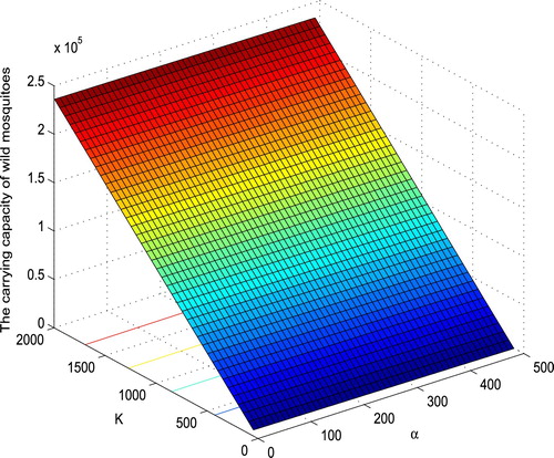
It is a challenging task to estimate the mating inhomogeneity constant α and the density-dependent competition constant K in the field. In order to estimate them and demonstrate the dependence of the threshold ${\delta }_A^{\ast }$ and the carrying capacity $A_2^{\ast }$ on the parameters, we assume that all the parameters are kept constant as follows unless otherwise specified [21,44], (30) $b=3,m=0.05,\tau =17.$(30) The basic assumption (5(5) $b_0=\frac{b}{m}-1>0.$(5) ) holds obviously. As shown in Figure 1, we note that $A_2^{\ast }$ increases almost linearly in K, and decreases almost linearly in α. Note that the magnitude of $A_2^{\ast }$ depends on the size of the studying area. Without loss of generality, we specify (31) $\alpha =100,K=1000.$(31) It is noticed that K and $A_2^{\ast }$ are dependent on the size of the release area. From (31(31) $\alpha =100,K=1000.$(31) ) we have $\begin{array}{r}{K}^{\ast }=4.3948,{\delta }_A^{\ast }=0.0114,A_1^{\ast }=3.4,A_2^{\ast }=58797.\end{array}$ As the unstable equilibrium $A_1^{\ast }$ is small, the migrating mosquitoes are easy to reach this threshold and then grow to the stable equilibrium $A_2^{\ast }$, which can explain the successful invading of Aedes albopictus in most tropical and subtropical areas.

Figure 1. The dependence of the carrying capacity $A_2^{\ast }$ of wild mosquitoes on α and K. With the parameters specified in (30(30) $b=3,m=0.05,\tau =17.$(30) ) and (31(31) $\alpha =100,K=1000.$(31) ), $A_2^{\ast }$ increases almost linearly in K, and decreases almost linearly in α.

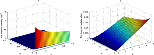
As shown in Figure 2 (A), with the increasing of α, ${\delta }_A^{\ast }$ decreases steeply for small α, and decreases steadily for large α. By fixing all the parameter values as in (30(30) $b=3,m=0.05,\tau =17.$(30) ) and (31(31) $\alpha =100,K=1000.$(31) ) except α, the simulation shows that ${\delta }_A^{\ast }$ decreases from 1.138 to 0.02231 when α increases from 1 to 50, and decreases from 0.02231 to 0.00291 when α increases from 50 to 400. However, ${\delta }_A^{\ast }$ decreases almost linearly with m, and increases almost linearly with b. For example, by fixing all the parameter values as in (30(30) $b=3,m=0.05,\tau =17.$(30) ) and (31(31) $\alpha =100,K=1000.$(31) ) except m, ${\delta }_A^{\ast }$ decreases from 0.01319 to 0.005986 as m increases from $\alpha =0.01$ to $\alpha =0.4$.

Figure 2. The dependence of the threshold mortality rate ${\delta }_A^{\ast }$ on α, b and m. The figure is simulated by (29(29) ${\delta }_A^{\ast }(\alpha ,b,m):=\frac{m}{K^{\ast }}=\frac{m}{2\alpha }{\left(\sqrt{\frac{b}{m}}-1\right)}^2.$(29) ) with the parameters specified in (30(30) $b=3,m=0.05,\tau =17.$(30) ) and (31(31) $\alpha =100,K=1000.$(31) ).

The threshold dynamics of the wild mosquito population remind us a feasible way to reduce the number of wild mosquitoes by raising its mortality rate. Applying insecticides is the traditional and most frequently used method of mosquito eradication in most countries in the world. Since insecticide spraying influences mainly the natural mortality rate of mosquitoes, we model the effect of insecticide spraying by raising the natural mortality rate m of adults. Consider the peak season of Aedes albopictus mosquitoes in which the population stabilizes at the steady-state level that coincides with the high-incidence of dengue in Guangzhou. We define the suppression rate γ as the ratio of the carrying capacity $A_2^{\ast }\left(m\right)$ of the inhabiting area with applying insecticides to that of without applying insecticides. We estimate the mortality rate m which is sufficient for $\gamma \le 5\mathrm{\%}$.

The carrying capacity $A_2^{\ast }\left(m\right)$ decreases gradually in m. Let m = 0.05 be the natural mortality rate of adult mosquitoes without interference of insecticides. Then $A_2^{\ast }\left(0.05\right)=58797$. If we double m to m = 0.1, then $A_2^{\ast }\left(0.1\right)=28793$, and so $\gamma =28793/58797=48.97\mathrm{\%}$. Similarly, as shown in Figure 3, we have $\gamma =14.93\mathrm{\%}$ for $A_2^{\ast }\left(0.3\right)=8777$ with m = 0.3, and $\gamma =4.93\mathrm{\%}$ for $A_2^{\ast }\left(0.72\right)=2898$ with m = 0.72. Hence, to reduce more than $95\mathrm{\%}$ of wild mosquitoes in the peak season, we need to spray insecticides so that the mortality rate m of adults above the level of 0.72. This indirect mosquito control method strongly depends on the effect of the insecticide.

Figure 3. The effect of insecticides spraying on wild mosquito population. Let $\phi \left(t\right)=500$ on $[-17,0]$, and the parameters, except m, be specified in (30(30) $b=3,m=0.05,\tau =17.$(30) ) and (31(31) $\alpha =100,K=1000.$(31) ). The curves simulated by (6(6) $\frac{\mathrm{d}A\left(t\right)}{\mathrm{d}t}=\frac{b{A}^2(t-\tau )}{2\alpha +A(t-\tau )}-m\left(1+\frac{A\left(t\right)}{K}\right)A\left(t\right),$(6) ) show that the steady-state level of wild mosquitoes decreases with m.

3.2. Threshold dynamics of compensation suppression policy

Although having an instant effect and being wildly used in the world, insecticide spraying is not long-term effective and sustainable method to control mosquitoes due to mosquito resistance to insecticides [3]. Recently, by using some special strains of Wolbachia pipientis, Xi et al. reduced more than 90% of the Aedes albopictus population in a field trial in Guangzhou [52]. The released Wolbachia-infected males keep their crossability in about three days in the field. Compensating the loss of crossable males by new releasing in every three days, we can maintain the number of crossable infected males in wild almost at a constant level. This compensation suppression policy can be modelled by setting $R\left(t\right)\equiv r\ge 0$ in (4(4) $\frac{\mathrm{d}A\left(t\right)}{\mathrm{d}t}=\frac{b{A}^2(t-\tau )}{2\alpha +A(t-\tau )+2R(t-\tau )}-m\left(1+\frac{A\left(t\right)+R\left(t\right)}{K}\right)A\left(t\right).$(4) ). 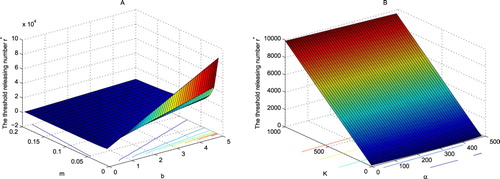For the case $K\le K^{\ast }$, Theorem 2.6 shows that the wild mosquitoes can be eliminated naturally when r>0. When $K>K^{\ast }$, Theorems 2.1–2.4 shows that $r^{\ast }$ defines the threshold releasing level above which all wild mosquitoes will be suppressed ultimately. As shown in Figure 4 (A), when $m\le 0.05$, $r^{\ast }$ increases steeply as m decreases from 0.05 to 0, or b increases from 1 to 5. However, $r^{\ast }$ varies steadily when m>0.05. Unlike b and m, as shown in Figure 4 (B), $r^{\ast }$ increases almost linearly with K, and decreases with α.

Figure 4. The dependence of the threshold releasing number $r^{\ast }$ on m, b, K and α. Let the parameters be specified in (30(30) $b=3,m=0.05,\tau =17.$(30) ) and (31(31) $\alpha =100,K=1000.$(31) ). (A) The nonlinear dependence of $r^{\ast }$ on m and b, (B) $r^{\ast }$ increases almost linearly in K, and decreases almost linearly in α.

With the parameters specified in (30(30) $b=3,m=0.05,\tau =17.$(30) ) and (31(31) $\alpha =100,K=1000.$(31) ), we have $K^{\ast }=4.3948$ and $r^{\ast }=9826$. Hence $K>K^{\ast }$. According to Theorems 2.1–2.4, (4(4) $\frac{\mathrm{d}A\left(t\right)}{\mathrm{d}t}=\frac{b{A}^2(t-\tau )}{2\alpha +A(t-\tau )+2R(t-\tau )}-m\left(1+\frac{A\left(t\right)+R\left(t\right)}{K}\right)A\left(t\right).$(4) ) displays similar dynamics to the wild mosquito population in this case, including bisability and semistability. Let the constant releasing number $r=5000<r^{\ast }$, as shown in Figure 5 (A), wild mosquitoes go to extinction when the initial mosquito population size $\phi \left(t\right)<A_1=1445$ on $[-17,0]$, while the mosquito suppression fails when $\phi \left(t\right)>A_1$ on $[-17,0]$ and the size of mosquito population tends to $A_2=42355$. Similarly, as shown in Figure 5(B) for the case $r=r^{\ast }$, the semistable dynamics shows that a successful population suppression is also dependent on the initial mosquito population size. It remains a rather subtle question to determine the ultimate fate of mosquito suppression when the initial functions cross over the unstable equilibrium $A_1$ or semistable equilibrium $A_1^{\ast }$.

Figure 5. The bistability and semistability of (4(4) $\frac{\mathrm{d}A\left(t\right)}{\mathrm{d}t}=\frac{b{A}^2(t-\tau )}{2\alpha +A(t-\tau )+2R(t-\tau )}-m\left(1+\frac{A\left(t\right)+R\left(t\right)}{K}\right)A\left(t\right).$(4) ). The parameters are specified in (30(30) $b=3,m=0.05,\tau =17.$(30) ) and (31(31) $\alpha =100,K=1000.$(31) ). (A) Let $R\left(t\right)\equiv 5000<r^{\ast }=9826$, (4(4) $\frac{\mathrm{d}A\left(t\right)}{\mathrm{d}t}=\frac{b{A}^2(t-\tau )}{2\alpha +A(t-\tau )+2R(t-\tau )}-m\left(1+\frac{A\left(t\right)+R\left(t\right)}{K}\right)A\left(t\right).$(4) ) displays bistability: $A\left(t\right)\to 0$ as $t\to \mathrm{\infty }$ when $\phi \left(t\right)<A_1=1445$ on $[-17,0]$, and $A\left(t\right)\to A_2=42355$ as $t\to \mathrm{\infty }$ when $\phi \left(t\right)>A_1=1445$ on $[-17,0]$. (B) With $R\left(t\right)\equiv r^{\ast }$, the unique positive equilibrium $A_1^{\ast }=14661$ is semistable, with $A\left(t\right)\to A_1^{\ast }$ as $t\to \mathrm{\infty }$ when $\phi \left(t\right)>A_1^{\ast }$ on $[-17,0]$.

3.3. The impact of temperature on suppression

As typical subtropical monsoon climate, Guangzhou has long hot and rainy summers, and warm and dry winters. As shown in Figure 6 (A), the daily mean temperatures of Guangzhou present strongly periodicity. A large number of experimental findings indicate that most of the life-table parameters of mosquitoes are strongly sensitive to climatic conditions, in particular, temperature and precipitations [10,26,38]. Deep understanding the mosquito-environment relationship is essential for the control of mosquito-borne diseases. To integrate temperature into our model, we introduce the temperature-dependent hatching rate of eggs ${\mu }_E$ [10,26,38] as $\begin{array}{r}{\mu }_E\left(T\right)=\frac{0.24\frac{273.15+T}{298}\exp \left[\frac{10798}{1.987}\left(\frac{1}{298}-\frac{1}{273.15+T}\right)\right]}{1+\exp \left[\frac{100000}{1.987}\left(\frac{1}{14184}-\frac{1}{273.15+T}\right)\right]}.\end{array}$ According to [8,9,38], the mean mortality rate in immature stage is estimated by $\begin{array}{r}{\delta }_I\left(T\right)=\left\{\begin{array}{ll}0.0000866T^2-0.00368T+0.09,& T\ge {12.5}^{\circ }C,\\ 0.5,& \mathrm{e}\mathrm{l}\mathrm{s}\mathrm{e}.\end{array}\right.\end{array}$ Hence the parameter b is given by (32) $b\left(T\right)=\frac{N{\mu }_E\left(T\right)}{2{\tau }_A}{e}^{-{\delta }_I\left(T\right)\tau },$(32) where N, ${\tau }_A$ and τ are defined in Table 1. Although the delays ${\tau }_A$ and τ are sensitive to temperature [10,26,38], our previous studies show that mosquito suppression does not sensitive to the delays, and so we assume them keep constants [19,22]. Furthermore, we estimate the natural mortality rate of adults by [8,9,38] (33) $m\left(T\right)=\left\{\begin{array}{ll}0.000114T^2-0.00427T+0.1278,& T\ge {15}^{\circ }C,\\ 0.5,& \mathrm{e}\mathrm{l}\mathrm{s}\mathrm{e}.\end{array}\right.$(33) We take January 1st as the initial time $t_0=0$ to display the significant seasonal variation of Aedes albopictus population. As shown in Figure 6 (B), the simulated curves generated by (4(4) $\frac{\mathrm{d}A\left(t\right)}{\mathrm{d}t}=\frac{b{A}^2(t-\tau )}{2\alpha +A(t-\tau )+2R(t-\tau )}-m\left(1+\frac{A\left(t\right)+R\left(t\right)}{K}\right)A\left(t\right).$(4) ) with the temperature-dependent parameters in (32(32) $b\left(T\right)=\frac{N{\mu }_E\left(T\right)}{2{\tau }_A}{e}^{-{\delta }_I\left(T\right)\tau },$(32) )–(33(33) $m\left(T\right)=\left\{\begin{array}{ll}0.000114T^2-0.00427T+0.1278,& T\ge {15}^{\circ }C,\\ 0.5,& \mathrm{e}\mathrm{l}\mathrm{s}\mathrm{e}.\end{array}\right.$(33) ) show a strong periodicity annually as the temperature, and capture several critical features of natural Aedes albopictus mosquito population in Guangzhou [29–31]. The eggs cannot hatch until the weekly average temperature rises to $10-{11}^{\circ }\mathrm{C}$, and the daily photoperiod reaches 11-11.5 h, which results in most of eggs laid after October accumulating into egg bank [30,37]. As the warm and rainy season starts in early March, the hatching of a large amount of diapause eggs leads to a rapid growth of Aedes albopictus population from early spring. The suitable temperature in the fall helps the population reaches its peak in late September and early October, after which the population size decays sharply and nearly vanishes from December to February in next year [30,31].

Figure 6. The Aedes albopictus population in Guangzhou shows strong periodicity annually as the temperature. (A) The daily mean temperature of Guangzhou from 2011 to 2017; Data source: China meteorological data sharing service system: http://www.cma.gov.cn/. (B) The simulated curve of wild Aedes albopictus population over a seven-year period in Guangzhou (2011–2017). With the parameters specified in (30(30) $b=3,m=0.05,\tau =17.$(30) ) and (31(31) $\alpha =100,K=1000.$(31) ), except $b\left(T\right)$ in (32(32) $b\left(T\right)=\frac{N{\mu }_E\left(T\right)}{2{\tau }_A}{e}^{-{\delta }_I\left(T\right)\tau },$(32) ) and $m\left(T\right)$ in (33(33) $m\left(T\right)=\left\{\begin{array}{ll}0.000114T^2-0.00427T+0.1278,& T\ge {15}^{\circ }C,\\ 0.5,& \mathrm{e}\mathrm{l}\mathrm{s}\mathrm{e}.\end{array}\right.$(33) ) being temperature-dependent functions, the curve is generated by (4(4) $\frac{\mathrm{d}A\left(t\right)}{\mathrm{d}t}=\frac{b{A}^2(t-\tau )}{2\alpha +A(t-\tau )+2R(t-\tau )}-m\left(1+\frac{A\left(t\right)+R\left(t\right)}{K}\right)A\left(t\right).$(4) ) with $\phi \left(t\right)=1000$ for $t\in [-17,0]$.

By the definitions, both of the threshold mortality rate ${\delta }_A^{\ast }$ and threshold releasing level $r^{\ast }$ are temperature-dependent, and so they vary in time. As shown in Figure 7, ${\delta }_A^{\ast }$ and $r^{\ast }$ display quasi-periodicity annually as temperature, and peaks in the period from July to October. Hence this period is the critical timing for the control of Aedes albopictus population by both chemical and biological measures.

Figure 7. The temperature dependence of the threshold mortality rate ${\delta }_A^{\ast }$ and threshold releasing level $r^{\ast }$. The curves are simulated by ${\delta }_A^{\ast }$ in (29(29) ${\delta }_A^{\ast }(\alpha ,b,m):=\frac{m}{K^{\ast }}=\frac{m}{2\alpha }{\left(\sqrt{\frac{b}{m}}-1\right)}^2.$(29) ) and $r^{\ast }$ in (7(7) $K^{\ast }=\frac{2\alpha }{b_0^2}(\sqrt{b_0+1}+1{)}^2,r^{\ast }=(3b_0+4)K-2\alpha -2\sqrt{2(b_0+1)\left[\right(b_0+2)K-\alpha ]K}.$(7) ) with the parameters specified in (30(30) $b=3,m=0.05,\tau =17.$(30) ) and (31(31) $\alpha =100,K=1000.$(31) ), except $b\left(T\right)$ in (32(32) $b\left(T\right)=\frac{N{\mu }_E\left(T\right)}{2{\tau }_A}{e}^{-{\delta }_I\left(T\right)\tau },$(32) ) and $m\left(T\right)$ in (33(33) $m\left(T\right)=\left\{\begin{array}{ll}0.000114T^2-0.00427T+0.1278,& T\ge {15}^{\circ }C,\\ 0.5,& \mathrm{e}\mathrm{l}\mathrm{s}\mathrm{e}.\end{array}\right.$(33) ). Both of ${\delta }_A^{\ast }$ and $r^{\ast }$ display quasi-periodicity annually as temperature, and take large values in the period from July to October.

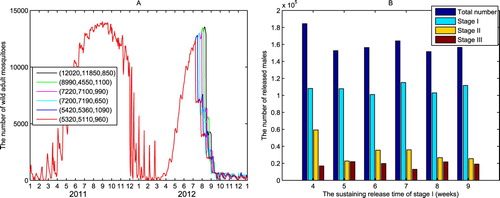
The coincidence of the high-incidence period of dengue fever with the peak season of Aedes albopictus population in Guangzhou indicates the close relation between mosquitoes size and dengue cases, so it is essential to reduce the wild mosquito population to a substantially lower level during the peak season of dengue. As shown in Figure 7 (B), the highest Aedes albopictus density in 2012 in Guangzhou was observed around September 12. We use our model to design suppression policy, aiming for the elimination of more than 95% mosquitoes in the peak season and keeping the effect until the end of November. We divide the suppression into three phases, a strong suppression phase with large releasing number (phase I) before September 12, followed by a transitional phase (phase II) after September 12 in about 15 days and a maintenance phase (phase III) after September 28 with small releasing number. In the field trial of mosquito suppression in Guangzhou, the infected males were released three times a week with constant amount [52]. In the simulation, we assume that $R\left(t\right)\equiv r_i>0$, i = 1, 2, 3 during the three phases, respectively.

To suppress the wild mosquito population during the peak season in the most cost-efficient way, we estimate the starting date of releasing and the least releasing amount. We initiate the simulation in January 1, 2011 to avoid the impact of initial mosquito population size on the estimation. The temporal profiles of adult mosquitoes shown in Figure 8(A) indicate that the number of wild mosquitoes decreases sharply after releasing, and more than $95\mathrm{\%}$ has been reduced at the peak. As shown in Figure 8 (B), although the values of $r_1$ reduce sharply with the increase of releasing time, the total releasing numbers of infected males in phase I varies in a small interval. When the highest mosquito density in September 12 has been suppressed by more than $95\mathrm{\%}$, it needs much fewer releasing number in the transitional phase II and maintenance phase III to keep the suppression level until the end of November. The variations of the total releasing numbers in phase II and III are insignificant as we expect. If the releasing starts five weeks ahead of the peak of mosquitoes instead of four weeks, the total releasing amount in all three phases reduces sharply from 184,430 to 152,630. However, the total releasing number has little variation when the length of phase I is shifted to 6, 7, 8, and 9 weeks, respectively, and keeps the lengths of the last two phases the same. The variation of the total releasing amount in three phases and its durations indicate that the most cost-efficient control should be started no less than 5 weeks before the start of the peak season of dengue.

Figure 8. Suppression of wild Aedes albopictus population in the high-incidence season of dengue fever. The curves are generated by (4(4) $\frac{\mathrm{d}A\left(t\right)}{\mathrm{d}t}=\frac{b{A}^2(t-\tau )}{2\alpha +A(t-\tau )+2R(t-\tau )}-m\left(1+\frac{A\left(t\right)+R\left(t\right)}{K}\right)A\left(t\right).$(4) ) with the same parameters as in Figure 6(B), except $R\left(t\right)\equiv r_1$ in phase I, $R\left(t\right)\equiv r_2$ in phase II, and $R\left(t\right)\equiv r_3$ in phase III. (A) A three phases releasing policy achieves the target of suppressing $95\mathrm{\%}$ of wild mosquitoes on September 12, 2012, and keeps the low density until the end of November. (B) The minimum constant releasing abundance in each phase and the total releasing number required to reach the target of suppression.

Acknowledgments

Thank the two anonymous reviewers very much for their valuable comments and suggestions which help us greatly improve the writing of this manuscript. This work was supported by National Natural Science Foundation of China (11471085, 11631005), Program for Changjiang Scholars and Innovative Research Team in University (IRT_16R16), and Natural Science Foundation of Guangdong Province (2017A030310597).

Disclosure statement

No potential conflict of interest was reported by the author(s).

Additional information

Funding

Thank the two anonymous reviewers very much for their valuable comments and suggestions which help us greatly improve the writing of this manuscript. This work was supported by National Natural Science Foundation of China [grant number 11471085], [grant number 11631005], and Natural Science Foundation of Guangdong Province [grant number 2017A030310597].

References

- F. Arkin, Dengue researcher faces charges in vaccine fiasco. Science 364(6438) (2019), pp. 320–320.
- M.P. Atkinson, Z. Su, N. Alphey, L.S. Alphey, P.G. Coleman, and L.M. Wein, Analyzing the control of mosquito-borne diseases by a dominant lethal genetic system, PNAS 104(22) (2007), pp. 9540–9545.
- F. Baldacchino, F. Caputo, A. Drago, T.A. Della, F. Montarsi, and A. Rizzoli, Control methods against invasive Aedes mosquitoes in Europe: a review, Pest. Manag. Sci. 71 (2015), pp. 1471–1485.
- S. Bhatt, P.W. Gething, O.J. Brady, J.P. Messina, A.W. Farlow, C.L. Moyes, J.M. Drake, J.S. Brownstein, A.G. Hoen, O. Sankoh, M.F. Myers, D.B. George, T. Jaenisch, G.R.W. Wint, C.P.Simmons, T.W. Scott, J.J. Farrar, and S.I. Hay, The global distribution and burden of dengue, Nature 496 (2013), pp. 504–507.
- M.S. Blagrove, C. Arias-Goata, A.B. Failloux, and S.P. Sinkins, Wolbachia strain wMel induces cytoplasmic incompatibility and blocks dengue transmission in Aedes albopictus, Proc. Natl. Acad. Sci. USA 109 (2012), pp. 255–260.
- L. Cai, S. Ai, and G. Fan, Dynamics of delayed mosquitoes populations models with two different strategies of releasing sterile mosquitoes, Math. Biosci. Eng. 15 (2018), pp. 1181–1202.
- L. Cai, S. Ai, and J. Li, Dynamics of mosquitoes populations with different strategies for releasing sterile mosquitoes, SIAM J. Appl. Math. 74(6) (2014), pp. 1786–1809.
- P. Cailly, A. Tran, T. Balenghien, G. L'Ambert, C. Toty, and P. Ezanno, A climate driven abundance model to assess mosquito control strategies, Ecol. Model. 227 (2012), pp. 7–17.
- Q. Cheng, Q. Jing, R.C. Spear, J.M. Marshall, Z. Yang, P. Gong, and S.V. Scarpino, Climate and the timing of imported cases as determinants of the dengue outbreak in Guangzhou, 2014: Evidence from a mathematical model, PLoS Negl. Trop. Dis. 10(2) (2016), p. e0004417.
- D.A. Focks, D.G. Haile, E. Daniels, and G.A. Mount, Dynamic life table model for Aedes aegypti (Diptera: Culicidae): simulation results and validation, J. Med. Entomol. 30(6) (1993), pp. 1018–1028.
- P.E. Fine, On the dynamics of symbiote-dependent cytoplasmic incompatibility in Culicine mosquitoes, J. Invertebr. Pathol 31(1) (1978), pp. 10–18.
- J.E. Gentile, S. Rund, and G.R. Madey, Modelling sterile insect technique to control the population of Anopheles gambiae, Malaria J. 14(1) (2015), p. 92.
- M. Hertig and S.B. Wolbach, Studies on rickettsia-like micro-organisms in insects, J. Med. Res. 44(3) (1924), pp. 329–374.
- L. Hu, M. Huang, M. Tang, J. Yu, and B. Zheng, Wolbachia spread dynamics in stochastic environments, Theor. Popul. Biol. 106 (2015), pp. 32–44.
- L. Hu, M. Tang, and Z. Wuet al, The threshold infection level for Wolbachia invasion in random environment. J. Diff. Equ. 266(7) (2019), pp. 4377–4393. Available at https://doi.org/10.1016/j.jde.2018.09.035.
- L. Hu, M. Huang, M. Tang, J. Yu, and B. Zheng, Wolbachia spread dynamics in multi-regimes of environmental conditions, J. Theor. Biol. 462 (2019), pp. 247–258.
- M. Huang, M. Tang, and J. Yu, Wolbachia infection dynamics by reaction-diffusion equations, Sci. China Math. 58 (2015), pp. 77–96.
- M. Huang, J. Yu, L. Hu, and B. Zheng, Qualitative analysis for a Wolbachia infection model with diffusion, Sci. China Math. 59 (2016), pp. 1249–1266.
- M. Huang, J. Lou, L. Hu, B. Zheng, and J. Yu, Assessing the efficiency of Wolbachia driven Aedes mosquito suppression by delay differential equations, J. Theor. Biol. 440 (2018), pp. 1–11.
- M. Huang, L. Hu, and B. Zheng, Comparing the efficiency of Wolbachia driven Aedes mosquito suppression strategies, J. Appl. Anal. Comput. 9(1) (2019), pp. 1–20.
- M. Huang, M. Tang, J. Yu, and B. Zheng, The impact of mating competitiveness and incomplete cytoplasmic incompatibility on Wolbachia-driven mosquito population suppression, Math. Bios. Eng. 16(5) (2019), pp. 4741–4757.
- M. Huang, M. Tang, J. Yu, and B. Zheng, A stage structured model of delay differential equations for Aedes mosquito population suppression, Discrete Contin. Dyn. Syst. 40(6) (2020), pp. 3467–3484.
- Y. Hui, G. Lin, J. Yu, and J. Li, A delayed differential equation model for mosquito population suppression with sterile mosquitoes, Discrete Contin. Dyn. Syst. Ser. B (2020). Available at https://doi.org/10.3934/dcdsb.2020118.
- P. Jia, X. Chen, J. Chen, L. Guo, X. Yu, and Q. Liu, A climate-driven mechanistic population model of Aedes albopictus with diapause, Para. Vect 9 (2016), p. 175.
- J.L. Kyle and E. Harris, Global spread and persistence of dengue, Annu. Rev. Microbiol. 62 (2008), pp. 71–92.
- R.M. Lana, M.M. Morais, T.F.M. de Lima, T.G.S. Carneiro, L.M. Stolerman, J.P.C. dos Santos, J.J.C. Corts, A.E. Eiras, C.T. Codeo, and L.A. Moreira, Assessment of a trap based Aedes aegypti surveillance program using mathematical modelling, PLoS One 13(1) (2018), p. e0190673.
- H. Laven, Cytoplasmic inheritance in culex, Nature 177 (1956), pp. 141–142.
- J. Li and S. Ai, Impusive releases of sterile mosquitoes and interactive dynamics with time delay, J. Biol. Dynam. 14(1) (2020), pp. 289–307.
- Y. Li, F. Kamara, G. Zhou, S. Puthiyakunnon, C. Li, Y. Liu, Y. Zhou, L. Yao, G. Yan, X. Chen, and P. Kittayapong, Urbanization increases Aedes albopictus larval habitats and accelerates mosquito development and survivorship, PLoS Negl. Trop. Dis. 8(11) (2014), p. e3301.
- F. Liu, C. Zhou, and P. Lin, Studies on the population ecology of Aedes albopictus 5. The seasonal abundance of natural population of Aedes albopictus in Guangzhou, Acta Sci. Natur. Universitatis Sunyatseni 29(2) (1990), pp. 118–122.
- F. Liu, C. Yao, P. Lin, and C. Zhou, Studies on life table of the natural population of Aedes albopictus, Acta Sci. Natur. Universitatis Sunyatseni 31(3) (1992), pp. 84–93.
- Y. Liu, Z. Guo, M. Smaily, and L. Wang, A Wolbachia infection model with free boundary, J. Biol. Dynam. 14(1) (2020), pp. 515–542.
- Z. Liu, Y. Zhang, and Y. Yang, Population dynamics of Aedes (Stegomyia) albopictus (Skuse) under laboratory conditions, Acta Entomol. Sin. 28(3) (1985), pp. 274–280.
- E.E. Ooi, K.T. Goh, and D.J. Gubler, Dengue prevention and 35 years of vector control in Singapore, Emerg. Infect. Diseases 12 (2006), pp. 887–893.
- P.A. Ross, M. Turelli, and A.A. Hoffmann, Evolutionary ecology of Wolbachia releases for disease control, Annu. Rev. Genet. 53 (2019), pp. 93–116.
- H.L. Smith, An Introduction to Delay Differential Equations with Applications to the Life Sciences, Springer, New York, Vol. 57, 2011.
- L. Toma, F. Severini, M. Luca, A. Bella, and R. Romi, Seasonal patterns of oviposition and egg hatching rate of Aedes albopiczus in Rome, J. Am. Mosq. Control. Assoc. 19(1) (2003), pp. 19–22.
- J. Waldock, N.L. Chandra, J. Lelieveld, Y. Proestos, E. Michael, G. Christophides, and P.E. Parham, The role of environment variables on Aedes albopictus biology and Chikungunya epidemiology, Pathogens Global Health. 107 (2013), pp. 224–240.
- T. Walker, P.H. Johnson, L.A. Moreika, I. Iturbe-Ormaetxe, F.D. Frentiu, C.J. Mcmeniman, Y.S. Leong, Y. Dong, A.L. Lloyd, S.A. Ritchie, S.L. O'Neill, and A.A. Hoffmann, The wMel Wolbachia strain blocks dengue and invades caged Aedes aegypti populations, Nature 476 (2011), pp. 450–453.
- E. Waltz, US reviews plan to infect mosquitoes with bacteria to stop disease, Nature 89(1) (2016), pp. 450–451.
- Y. Wang, X. Liu, C. Li, T. Su, J. Jin, Y. Guo, D. Ren, Z. Yang, and F Meng, A survey of insecticide resistance in Aedes albopictus (Diptera: Culicidae) during a 2014 dengue fever outbreak in Guangzhou, China, China. J. Econ. Entomol. 110(1) (2017), pp. 239–244.
- WHO, Global strategy for dengue prevention and control 2012–2020. Geneva: World Health Organization, 2012.
- Z. Xi, C.C. Khoo, and S.L. Dobson, Wolbachia establishment and invasion in an Aedes aegypti laboratory population, Science 310 (2005), pp. 326–328.
- J. Yu, Modeling mosquito population suppression based on delay differential equations, SIAM J. Appl. Math. 78(6) (2018), pp. 3168–3187.
- J. Yu and J. Li, Dynamics of interactive wild and sterile mosquitoes with time delay, J. Biol. Dynam.13(1) (2019), pp. 606–620.
- J. Yu and J. Li, Global asymptotic stability in an interactive wild and sterile mosquito model, J. Diff. Equ. 269(7) (2020), pp. 6193–6215.
- J. Yu and B. Zheng, Modeling Wolbachia infection in mosquito population via discrete dynamical models, J. Diff. Equ. Appl. 25 (2019), pp. 1549–1567.
- L. Zhang, L. Tan, H. Ai, C. Lei, and F. Yuan, Laboratory and field studies on the oviposition pattern of Aedes albopictus, Acta Parasitol. Et. Med. Entomol. Sin. 16 (2009), pp. 219–223.
- B. Zheng, M. Tang, and J. Yu, Modeling Wolbachia spread in mosquitoes through delay differential equation, SIAM J. Appl. Math. 74 (2014), pp. 743–770.
- B. Zheng and J. Yu, Characterization of Wolbachia enhancing domain in mosquitoes with imperfect maternal transmission, J. Biol. Dynam. 12(1) (2018), pp. 596–610.
- B. Zheng, J. Yu, Z. Xi, and M. Tang, The annual abundance of dengue and Zika vector Aedes albopictus and its stubbornness to suppression, Ecol. Model. 387 (2018), pp. 38–48.
- X. Zheng, D. Zhang, Y. Li, C. Yang, Y. Wu, X. Liang, Y. Liang, X. Pan, L. Hu, Q. Sun, X. Wang, Y. Wei, J. Zhu, W. Qian, Z. Yan, A.G. Parker, J.R.L. Gilles, K. Bourtzis, J. Bouyer, M. Tang, B. Zheng, J. Yu, J. Liu, J. Zhuang, Z. Hu, M. Zhang, J. Gong, X. Hong, Z. Zhang, L. Lin, Q. Liu, Z. Hu, Z. Wu, L.A. Baton, A.A. Hoffmann, and Z. Xi, Incompatible and sterile insect techniques combined eliminate mosquitoes, Nature 572 (2019), pp. 56–61.
- Z. Zhong and G. He, The life table of laboratory Aedes albopictus under various temperatures, Academic J. Sun Yat-sen University Medical Sci. 9(3) (1988), pp. 35–39.
- Z. Zhong and G. He, The life and fertility table of Aedes albopictus under different temperatures, Acta Entom. Sinica 33(1) (1990), pp. 64–70.