Analysis and prediction of the COVID-19 outbreak in Pakistan

Abstract

In this study, we estimate the severity of the COVID-19 outbreak in Pakistan prior to and after lockdown restrictions were eased. We also project the epidemic curve considering realistic quarantine, social distancing and possible medication scenarios. The pre-lock down value of ${\mathcal{R}}_0$ is estimated to be 1.07 and the post lock down value is estimated to be 1.86. Using this analysis, we project the epidemic curve. We note that if no substantial efforts are made to contain the epidemic, it will peak in mid-September, 2020, with the maximum projected active cases being close to 700, 000. In a realistic, best case scenario, we project that the epidemic peaks in early to mid-July, 2020, with the maximum active cases being around 120, 000. We note that social distancing measures and medication will help flatten the curve; however, without the reintroduction of further lock down, it would be very difficult to make ${\mathcal{R}}_0<1$.

Keywords:

• COVID-19
• coronavirus
• medication
• prediction
• projection
• epidemic curve

1. Introduction

Coronavirus disease (COVID-19) is a respiratory tract illness which originated in Wuhan, China in early December 2019. It spread to other countries in Asia, Europe and North America in early 2020 and was declared a pandemic by the WHO on 11 March 2020. As of 15 June 2020, the disease is prevalent in at least 212 countries and territories, with more than 8 million cases reported and around 435,000 fatalities [31].

COVID-19 is caused by a coronavirus SARS-CoV-2 [30], belonging to a family of viruses that are found in humans and different species of animals including cattle, camels and bats. These have in the past caused serious disease outbreaks in human populations as happened in MERS (caused by MERS-CoV) and SARS (caused by SARS-CoV) [5,14,21].

The virus spreads primarily from person to person through respiratory droplets [5]. Symptoms of the disease may appear 2–14 days after exposure and may include fever, cough, shortness of breath, chills, muscle pain and loss of taste or smell[15,30]. These may range from very mild (in 80% of the cases) to severe (in 15% of the cases) to critical (in 5% of the cases) [30]. Those at higher risk for severe illness include the elderly (people aged 65 and above) and people with comorbidities such as chronic lung diseases, diabetes, chronic kidney diseases, serious heart conditions and immunocompromised individuals [32].

At this time, there is no approved vaccine for COVID-19 although some possible vaccines are undergoing clinical trials [28]. Several antiviral drugs are now in advanced clinical trial phase [4,13,16,25,29]. The trials for these drugs have so far have produced mixed results with some drug regimens showing encouraging outcomes, such as shortening of the duration of the disease, while others showing no significant change in the outcomes due to medication. A drug that has been suggested to have beneficial effects in COVID-19 treatment is Remdesivir, in their study Grein et al. [13] have reported improvement in 68 % of the patients in a controlled trial using Remdesivir, similarly Beigel et al. [4] have also reported shortening in the time to recovery with Remdesivir use. In another study involving triple antiviral therapy, Huang et al. [15] have also reported alleviation of symptoms and a shortening of the duration of the disease. At the time of writing, Remdesivir has received emergency approval in few countries [11].

Non-pharmaceutical interventions such as social distancing measures, isolation and quarantine had a positive effect in controlling the outbreak. However, these measures, specially lock downs, also resulted in substantial economic and social cost [19] and as a consequence countries are easing the lock downs. For this reason, in the near future, social distancing and the availability of medication are the viable strategies that can be used to control the epidemic.

After the initial outbreak in China, the COVID-19 spread world wide, with Europe becoming the initial epicenter of the outbreak [30], followed by the USA, South Asia, India and Pakistan with cases being reported in early March 2020 have had a very different epidemic curve as compared to China, Europe and North America, with much lower disease burden and mortality. There has been much speculation as to why the outbreak has been so different in these countries, from more mundane theories citing effective and early quarantine and isolation, demographics and higher temperatures to more esoteric ones that hold a better immune response or previous vaccinations (which are no longer required in the West) as possible reasons. However, to our knowledge, no proper study has been undertaken and all of these are conjectures at the moment. As these countries have eased lock downs, the COVID-19 cases have started to increase at a high rate, morbidity though still remains low as compared to other countries [20].

Since the outbreak, many studies have been undertaken to estimate the growth rates and understand the transmission dynamics of COVID-19. These include phenomenological models [33], stochastic models [17], both of which are very useful in the early stages of the outbreak, and mechanistic models [3,6,9,18,22] that incorporate our understanding of the transmission pathways. Imran et al. [2] and Perkins et al. [23] have used optimal control techniques to propose efficient control strategies. Gumel et al. [9] have considered the impact of various non-pharmaceutical interventions on the disease burden and mortality. The aim of such modelling is twofold: (1) to provide estimates of the severity of the outbreak by calculating quantities like the growth trends of the epidemic and estimates of the final outbreak size and duration of the outbreak and (2) to provide insights into efficacy of various control measures.

The COVID-19 epidemic in Pakistan started in early March 2020, with the initial cases being reported in late February 2020. Lock downs that were imposed in different parts of the country in the third week of March in order to control the outbreak were successful in keeping the disease numbers low. However with the start of the Muslim holy month of Ramadan on 24 April, the lock down measure became less effective and by 1 May the lock down restriction were officially eased with complete relaxation on 22 May. As expected, this led to an upsurge in the infections with close to 80,000 active cases and around 132,000 total cases being reported by 12 June. Considering the situation on 10 June, the WHO issued an advisory strongly recommending an intermittent lock down for the following two weeks.

In this study, we model the COVID 19 outbreak using a variant of the models proposed by Imran et al. [1,2] for the transmission dynamics of the disease. This model incorporates compartments for quarantined, isolated, and asymptomatic individuals, pathways considered important in transmission of the disease. We also include a compartment for individuals taking medication as we would like to study the possible effects of medication in controlling the disease. The dynamics of the COVID 19 outbreak in Pakistan have been qualitatively different before and after the lock down was eased. We estimate the value of ${\mathcal{R}}_0$ in Pakistan for the two different phases of the outbreak, noting that during this time no medication was available. We then project the disease curve considering minimal intervention as well as various control strategies. At the moment, the viable strategies for controlling the outbreak are quarantine, isolation, social distancing and possibly medication. In fact, there have been emergency approvals for different treatments for the disease in various countries including Pakistan. We project the epidemic curve considering various quarantine, social distancing and medication scenarios. We note that the most effective control measure is a lock down but a very strict lock down does not seem to be an option that is being considered by the government. However, a moderate and intermittent lock down may be possible. Further, by making sure social distancing protocols issued by the government are followed we can reduce the contact rate to varying degrees and flatten the disease curve. Finally, we consider various medication scenarios. As mentioned, medication to date has, to varying degrees, reduced the time of infection as well as alleviate symptoms. We consider medications primarily in the context of shortening of the time of infection which thereby helps to bring the disease numbers down. We look at various levels of quarantine, social distancing and medication to study how each of these would affect the disease numbers and when the infected numbers would peak. We conclude the study by summarizing our findings and suggesting realistic control measures with their impact on the epidemic.

2. Model formulation

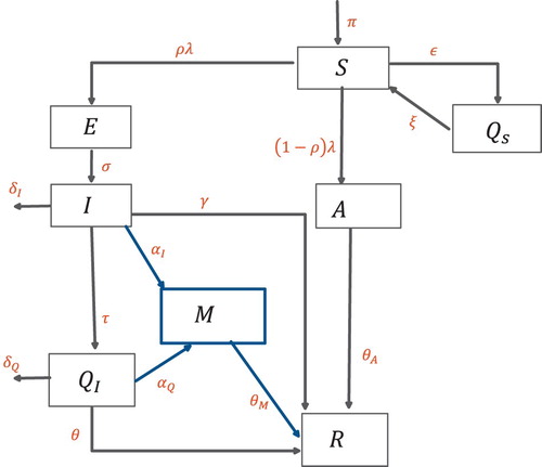
The COVID-19 transmission model we consider is based upon the SEIR model and takes into account the effects of quarantine, isolation, medication and asymptomatic individuals. The total population $N(t)$ is divided into eight mutually exclusive subpopulations, susceptibles S, these are individuals who can fall ill by coming in contact with an infected individual, quarantined susceptibles $Q_S$, these individuals are removed from the susceptible group at rate ε, either through self quarantined or lock-down measures, they, however, go back to the susceptible group at rate ξ. The susceptibles move to the exposed class by coming in contact with any infectious individual, at rate $\rho \lambda$, some exposed individuals will not show symptoms and are accounted for in the model by the movement to the asymptomatic class at rate $(1-\rho )\lambda$. Exposed individuals E become infected at rate σ. Infected individuals I can be isolated or given medication at a rate of τ and ${\alpha }_I$, whereas a fraction of isolated $Q_I$ are given medication at rate ${\alpha }_Q$. The individuals taking medication are represented by a separate compartment M, these include individuals from the isolated and infected classes who are under treatment. Based on clinical trials thus far, the main effect of medication we incorporate is that, it shortens the duration of the disease [4,13,15]. The recovery time for infected I, asymptomatic A, isolation $Q_I$ and medication M is given by $1/\gamma$,$1/{\theta }_A$,$1/\theta$ and $1/{\theta }_M$, respectively. The schematic of the transmission pathways is given in Figure 1. The total population $N(t)$ is given by the sum of the subpopulations. (1) $N(t)=S(t)+Q_S(t)+E(t)+I(t)+A(t)+Q_I(t)+M(t)+R(t)$(1) The governing equations are given below. (2) $\begin{array}{rl}\frac{\mathrm{d}S}{\mathrm{d}t}& =\mathrm{\Pi }+\xi Q_S-(\lambda +\mu +ϵ)S\\ \frac{\mathrm{d}{Q}_S}{\mathrm{d}t}& =ϵS-(\xi +\mu )Q_S\\ \frac{\mathrm{d}E}{\mathrm{d}t}& =\rho \lambda S-(\sigma +\mu )E\\ \frac{\mathrm{d}I}{\mathrm{d}t}& =\sigma E-({\delta }_I+\tau +{\alpha }_I+\mu +\gamma )I\\ \frac{\mathrm{d}A}{\mathrm{d}t}& =(1-\rho )\lambda S-({\theta }_A+\mu )A\\ \frac{\mathrm{d}{Q}_I}{\mathrm{d}t}& =\tau I-(\theta +{\alpha }_Q+{\delta }_Q+\mu )Q_I\\ \frac{\mathrm{d}M}{\mathrm{d}t}& ={\alpha }_{I}I+{\alpha }_Q{Q}_I-({\theta }_M+\mu )M\\ \frac{\mathrm{d}R}{\mathrm{d}t}& =\theta Q_I+\gamma I+{\theta }_{A}A+{\theta }_{M}M-\mu R\end{array}$(2) where λ is the force of infection. (3) $\lambda =\frac{\beta }{N}(I+{\eta }_1{Q}_I+{\eta }_{2}A++{\eta }_{4}M)$(3) Here β is the effective contact rate, where as ${\eta }_1$,${\eta }_2$ and ${\eta }_4$ are the associated relative infectiousness parameters for the $Q_I$,A and M subpopulations. Tables 2 and 3 represent the description of variables and parameters of the model and are given in the Appendix.

Figure 1. Schematic diagram of the model (2(2) $\begin{array}{rl}\frac{\mathrm{d}S}{\mathrm{d}t}& =\mathrm{\Pi }+\xi Q_S-(\lambda +\mu +ϵ)S\\ \frac{\mathrm{d}{Q}_S}{\mathrm{d}t}& =ϵS-(\xi +\mu )Q_S\\ \frac{\mathrm{d}E}{\mathrm{d}t}& =\rho \lambda S-(\sigma +\mu )E\\ \frac{\mathrm{d}I}{\mathrm{d}t}& =\sigma E-({\delta }_I+\tau +{\alpha }_I+\mu +\gamma )I\\ \frac{\mathrm{d}A}{\mathrm{d}t}& =(1-\rho )\lambda S-({\theta }_A+\mu )A\\ \frac{\mathrm{d}{Q}_I}{\mathrm{d}t}& =\tau I-(\theta +{\alpha }_Q+{\delta }_Q+\mu )Q_I\\ \frac{\mathrm{d}M}{\mathrm{d}t}& ={\alpha }_{I}I+{\alpha }_Q{Q}_I-({\theta }_M+\mu )M\\ \frac{\mathrm{d}R}{\mathrm{d}t}& =\theta Q_I+\gamma I+{\theta }_{A}A+{\theta }_{M}M-\mu R\end{array}$(2) ).

3. Basic properties

$S,Q_S,E,I,A,Q_I,M,R$, respectively, for all $t\ge 0$. Moreover, it satisfies the following inequality of boundedness.

Lemma 3.1

The closed set: $\mathcal{B}=\{(S,Q_S,E,I,A,Q_I,M,R)\in {\mathbb{R}}_{+}^8:S+Q_S+E+I+A+Q_I+M+R\le \frac{\mathrm{\Pi }}{\mu }\}$ is positively invariant.

Proof is attached in the Appendix.

4. Steady-state analysis

4.1. Disease-free equilibrium

The model (2(2) $\begin{array}{rl}\frac{\mathrm{d}S}{\mathrm{d}t}& =\mathrm{\Pi }+\xi Q_S-(\lambda +\mu +ϵ)S\\ \frac{\mathrm{d}{Q}_S}{\mathrm{d}t}& =ϵS-(\xi +\mu )Q_S\\ \frac{\mathrm{d}E}{\mathrm{d}t}& =\rho \lambda S-(\sigma +\mu )E\\ \frac{\mathrm{d}I}{\mathrm{d}t}& =\sigma E-({\delta }_I+\tau +{\alpha }_I+\mu +\gamma )I\\ \frac{\mathrm{d}A}{\mathrm{d}t}& =(1-\rho )\lambda S-({\theta }_A+\mu )A\\ \frac{\mathrm{d}{Q}_I}{\mathrm{d}t}& =\tau I-(\theta +{\alpha }_Q+{\delta }_Q+\mu )Q_I\\ \frac{\mathrm{d}M}{\mathrm{d}t}& ={\alpha }_{I}I+{\alpha }_Q{Q}_I-({\theta }_M+\mu )M\\ \frac{\mathrm{d}R}{\mathrm{d}t}& =\theta Q_I+\gamma I+{\theta }_{A}A+{\theta }_{M}M-\mu R\end{array}$(2) ) achieves the disease-free equilibrium (DFE) whenever there is no induction of infection by the disease, i.e. the force of infection is zero, $\lambda =0$. Mathematically, this can be calculated by equating the right hand side of (2(2) $\begin{array}{rl}\frac{\mathrm{d}S}{\mathrm{d}t}& =\mathrm{\Pi }+\xi Q_S-(\lambda +\mu +ϵ)S\\ \frac{\mathrm{d}{Q}_S}{\mathrm{d}t}& =ϵS-(\xi +\mu )Q_S\\ \frac{\mathrm{d}E}{\mathrm{d}t}& =\rho \lambda S-(\sigma +\mu )E\\ \frac{\mathrm{d}I}{\mathrm{d}t}& =\sigma E-({\delta }_I+\tau +{\alpha }_I+\mu +\gamma )I\\ \frac{\mathrm{d}A}{\mathrm{d}t}& =(1-\rho )\lambda S-({\theta }_A+\mu )A\\ \frac{\mathrm{d}{Q}_I}{\mathrm{d}t}& =\tau I-(\theta +{\alpha }_Q+{\delta }_Q+\mu )Q_I\\ \frac{\mathrm{d}M}{\mathrm{d}t}& ={\alpha }_{I}I+{\alpha }_Q{Q}_I-({\theta }_M+\mu )M\\ \frac{\mathrm{d}R}{\mathrm{d}t}& =\theta Q_I+\gamma I+{\theta }_{A}A+{\theta }_{M}M-\mu R\end{array}$(2) ) to zero with $\lambda =0$. Let ${\mathcal{F}}_0$ represent the DFE of the model. $\begin{array}{rl}{\mathcal{F}}_0& =(S^{\ast },Q_S^{\ast },E^{\ast },I^{\ast },A^{\ast },Q_I^{\ast },M^{\ast },R^{\ast })\\ {\mathcal{F}}_0& =(\frac{\pi (\mu +\xi )}{\mu (\mu +\xi +ϵ)},\frac{\pi ϵ}{\mu (\mu +\xi +ϵ)},0,0,0,0,0,0)\end{array}$ The local stability of DFE is quantified by a threshold quantity ${\mathcal{R}}_0$ which can be found by means of the next generation operator method [27].

4.2. The basic reproduction number ${\mathcal{R}}_0$

The threshold quantity $\mathcal{R}$ represents the average number of new secondary infections produced by the single infection in a completely susceptible population. It can be obtained by calculating the spectral radius of the $F{V}^{-1}$ matrix from the next generation method [27]. The associated F and V matrices of model (2(2) $\begin{array}{rl}\frac{\mathrm{d}S}{\mathrm{d}t}& =\mathrm{\Pi }+\xi Q_S-(\lambda +\mu +ϵ)S\\ \frac{\mathrm{d}{Q}_S}{\mathrm{d}t}& =ϵS-(\xi +\mu )Q_S\\ \frac{\mathrm{d}E}{\mathrm{d}t}& =\rho \lambda S-(\sigma +\mu )E\\ \frac{\mathrm{d}I}{\mathrm{d}t}& =\sigma E-({\delta }_I+\tau +{\alpha }_I+\mu +\gamma )I\\ \frac{\mathrm{d}A}{\mathrm{d}t}& =(1-\rho )\lambda S-({\theta }_A+\mu )A\\ \frac{\mathrm{d}{Q}_I}{\mathrm{d}t}& =\tau I-(\theta +{\alpha }_Q+{\delta }_Q+\mu )Q_I\\ \frac{\mathrm{d}M}{\mathrm{d}t}& ={\alpha }_{I}I+{\alpha }_Q{Q}_I-({\theta }_M+\mu )M\\ \frac{\mathrm{d}R}{\mathrm{d}t}& =\theta Q_I+\gamma I+{\theta }_{A}A+{\theta }_{M}M-\mu R\end{array}$(2) ) are as follows $\begin{array}{rl}F& =\left(\begin{array}{ccccc}0& {\displaystyle \frac{\beta \rho S^{\ast }}{N^{\ast }}}& {\displaystyle \frac{\beta \rho {\eta }_2{S}^{\ast }}{N^{\ast }}}& {\displaystyle \frac{\beta \rho {\eta }_1{S}^{\ast }}{N^{\ast }}}& {\displaystyle \frac{\beta \rho {\eta }_4{S}^{\ast }}{N^{\ast }}}\\ 0& 0& 0& 0& 0\\ 0& {\displaystyle \frac{\beta (1-\rho )S^{\ast }}{N^{\ast }}}& {\displaystyle \frac{\beta (1-\rho ){\eta }_2{S}^{\ast }}{N^{\ast }}}& {\displaystyle \frac{\beta (1-\rho ){\eta }_1{S}^{\ast }}{N^{\ast }}}& {\displaystyle \frac{\beta (1-\rho ){\eta }_4{S}^{\ast }}{N^{\ast }}}\\ 0& 0& 0& 0& 0\\ 0& 0& 0& 0& 0\end{array}\right),\\ V& =\left(\begin{array}{ccccc}{k}_1& 0& 0& 0& 0\\ -\sigma & k_2& 0& 0& 0\\ 0& 0& k_3& 0& 0\\ 0& -\tau & 0& k_4& 0\\ 0& -{\alpha }_I& 0& -{\alpha }_Q& k_5\end{array}\right)\end{array}$ where $k_1=\sigma +\mu$, $k_2={\delta }_I+\tau +\gamma +{\alpha }_I+\mu$, $k_3={\theta }_A+\mu$, $k_4=\theta +{\delta }_Q+{\alpha }_Q+\mu$, $k_5={\theta }_M+\mu$ (4) ${\mathcal{R}}_0=\frac{\beta (\mu +\xi )}{\mu +\xi +ϵ}[(1-\rho )\frac{{\eta }_2}{k_3}+\rho \left(\frac{\sigma }{k_1{k}_2}\right)(\frac{{\eta }_4(k_4{\alpha }_I+\tau {\alpha }_Q)}{k_4{k}_5}+\frac{{\eta }_1\tau }{k_4}+1)]$(4)

Stability of DFE

Lemma 4.1

The steady-state (DFE) ${\mathcal{F}}_0$ of the model (2(2) $\begin{array}{rl}\frac{\mathrm{d}S}{\mathrm{d}t}& =\mathrm{\Pi }+\xi Q_S-(\lambda +\mu +ϵ)S\\ \frac{\mathrm{d}{Q}_S}{\mathrm{d}t}& =ϵS-(\xi +\mu )Q_S\\ \frac{\mathrm{d}E}{\mathrm{d}t}& =\rho \lambda S-(\sigma +\mu )E\\ \frac{\mathrm{d}I}{\mathrm{d}t}& =\sigma E-({\delta }_I+\tau +{\alpha }_I+\mu +\gamma )I\\ \frac{\mathrm{d}A}{\mathrm{d}t}& =(1-\rho )\lambda S-({\theta }_A+\mu )A\\ \frac{\mathrm{d}{Q}_I}{\mathrm{d}t}& =\tau I-(\theta +{\alpha }_Q+{\delta }_Q+\mu )Q_I\\ \frac{\mathrm{d}M}{\mathrm{d}t}& ={\alpha }_{I}I+{\alpha }_Q{Q}_I-({\theta }_M+\mu )M\\ \frac{\mathrm{d}R}{\mathrm{d}t}& =\theta Q_I+\gamma I+{\theta }_{A}A+{\theta }_{M}M-\mu R\end{array}$(2) ) is locally asymptotically stable if ${\mathcal{R}}_0<1,$ and unstable if ${\mathcal{R}}_0>1$ [27].

This Lemma implies that a small influx of infected will not lead to a bigger outbreak and the disease will become extinct in long run.

More concretely, this means that disease extinction is independent of the initial subpopulations in model (2(2) $\begin{array}{rl}\frac{\mathrm{d}S}{\mathrm{d}t}& =\mathrm{\Pi }+\xi Q_S-(\lambda +\mu +ϵ)S\\ \frac{\mathrm{d}{Q}_S}{\mathrm{d}t}& =ϵS-(\xi +\mu )Q_S\\ \frac{\mathrm{d}E}{\mathrm{d}t}& =\rho \lambda S-(\sigma +\mu )E\\ \frac{\mathrm{d}I}{\mathrm{d}t}& =\sigma E-({\delta }_I+\tau +{\alpha }_I+\mu +\gamma )I\\ \frac{\mathrm{d}A}{\mathrm{d}t}& =(1-\rho )\lambda S-({\theta }_A+\mu )A\\ \frac{\mathrm{d}{Q}_I}{\mathrm{d}t}& =\tau I-(\theta +{\alpha }_Q+{\delta }_Q+\mu )Q_I\\ \frac{\mathrm{d}M}{\mathrm{d}t}& ={\alpha }_{I}I+{\alpha }_Q{Q}_I-({\theta }_M+\mu )M\\ \frac{\mathrm{d}R}{\mathrm{d}t}& =\theta Q_I+\gamma I+{\theta }_{A}A+{\theta }_{M}M-\mu R\end{array}$(2) ).

4.3. Endemic equilibrium

The equilibrium state of the system (2(2) $\begin{array}{rl}\frac{\mathrm{d}S}{\mathrm{d}t}& =\mathrm{\Pi }+\xi Q_S-(\lambda +\mu +ϵ)S\\ \frac{\mathrm{d}{Q}_S}{\mathrm{d}t}& =ϵS-(\xi +\mu )Q_S\\ \frac{\mathrm{d}E}{\mathrm{d}t}& =\rho \lambda S-(\sigma +\mu )E\\ \frac{\mathrm{d}I}{\mathrm{d}t}& =\sigma E-({\delta }_I+\tau +{\alpha }_I+\mu +\gamma )I\\ \frac{\mathrm{d}A}{\mathrm{d}t}& =(1-\rho )\lambda S-({\theta }_A+\mu )A\\ \frac{\mathrm{d}{Q}_I}{\mathrm{d}t}& =\tau I-(\theta +{\alpha }_Q+{\delta }_Q+\mu )Q_I\\ \frac{\mathrm{d}M}{\mathrm{d}t}& ={\alpha }_{I}I+{\alpha }_Q{Q}_I-({\theta }_M+\mu )M\\ \frac{\mathrm{d}R}{\mathrm{d}t}& =\theta Q_I+\gamma I+{\theta }_{A}A+{\theta }_{M}M-\mu R\end{array}$(2) ) in the presence of the infection, i.e. $\lambda \ne 0$ is known as the endemic equilibrium. Let ${\mathcal{F}}_1$ represent the endemic equilibrium of the model (2(2) $\begin{array}{rl}\frac{\mathrm{d}S}{\mathrm{d}t}& =\mathrm{\Pi }+\xi Q_S-(\lambda +\mu +ϵ)S\\ \frac{\mathrm{d}{Q}_S}{\mathrm{d}t}& =ϵS-(\xi +\mu )Q_S\\ \frac{\mathrm{d}E}{\mathrm{d}t}& =\rho \lambda S-(\sigma +\mu )E\\ \frac{\mathrm{d}I}{\mathrm{d}t}& =\sigma E-({\delta }_I+\tau +{\alpha }_I+\mu +\gamma )I\\ \frac{\mathrm{d}A}{\mathrm{d}t}& =(1-\rho )\lambda S-({\theta }_A+\mu )A\\ \frac{\mathrm{d}{Q}_I}{\mathrm{d}t}& =\tau I-(\theta +{\alpha }_Q+{\delta }_Q+\mu )Q_I\\ \frac{\mathrm{d}M}{\mathrm{d}t}& ={\alpha }_{I}I+{\alpha }_Q{Q}_I-({\theta }_M+\mu )M\\ \frac{\mathrm{d}R}{\mathrm{d}t}& =\theta Q_I+\gamma I+{\theta }_{A}A+{\theta }_{M}M-\mu R\end{array}$(2) ). (5) ${\mathcal{F}}_1=(S^{\ast \ast },Q_S^{\ast \ast },E^{\ast \ast },I^{\ast \ast },A^{\ast \ast },Q_I^{\ast \ast },M^{\ast \ast },R^{\ast \ast })$(5) Further,The force of infection λ can be written in terms of the equilibrium as ${\lambda }^{\ast \ast }={\displaystyle \frac{\beta }{N^{\ast \ast }}}(I^{\ast \ast }+{\eta }_1{Q}_I^{\ast \ast }+{\eta }_2{A}^{\ast \ast }+{\eta }_4{M}^{\ast \ast })$ with $N^{\ast \ast }=S^{\ast \ast }+Q_S^{\ast \ast }+E^{\ast \ast }+I^{\ast \ast }+A^{\ast \ast }+Q_I^{\ast \ast }+M^{\ast \ast }+R^{\ast \ast }$

Solving the system (2(2) $\begin{array}{rl}\frac{\mathrm{d}S}{\mathrm{d}t}& =\mathrm{\Pi }+\xi Q_S-(\lambda +\mu +ϵ)S\\ \frac{\mathrm{d}{Q}_S}{\mathrm{d}t}& =ϵS-(\xi +\mu )Q_S\\ \frac{\mathrm{d}E}{\mathrm{d}t}& =\rho \lambda S-(\sigma +\mu )E\\ \frac{\mathrm{d}I}{\mathrm{d}t}& =\sigma E-({\delta }_I+\tau +{\alpha }_I+\mu +\gamma )I\\ \frac{\mathrm{d}A}{\mathrm{d}t}& =(1-\rho )\lambda S-({\theta }_A+\mu )A\\ \frac{\mathrm{d}{Q}_I}{\mathrm{d}t}& =\tau I-(\theta +{\alpha }_Q+{\delta }_Q+\mu )Q_I\\ \frac{\mathrm{d}M}{\mathrm{d}t}& ={\alpha }_{I}I+{\alpha }_Q{Q}_I-({\theta }_M+\mu )M\\ \frac{\mathrm{d}R}{\mathrm{d}t}& =\theta Q_I+\gamma I+{\theta }_{A}A+{\theta }_{M}M-\mu R\end{array}$(2) ), the endemic equilibrium becomes (6) $\begin{array}{rl}{S}^{\ast \ast }& =\frac{\pi (\mu +\xi )}{({\lambda }^{\ast \ast }+\mu )(\mu +\xi )+\mu ϵ};Q_s^{\ast \ast }=\frac{\pi ϵ}{({\lambda }^{\ast \ast }+\mu )(\mu +\xi )+\mu ϵ}\\ E^{\ast \ast }& =\frac{\pi {\lambda }^{\ast \ast }\rho (\mu +\xi )}{k_1(({\lambda }^{\ast \ast }+\mu )(\mu +\xi )+\mu ϵ)};I^{\ast \ast }=\frac{\pi {\lambda }^{\ast \ast }\rho \sigma (\mu +\xi )}{k_1{k}_3(({\lambda }^{\ast \ast }+\mu )(\mu +\xi )+\mu ϵ)}\\ A^{\ast \ast }& =\frac{\pi {\lambda }^{\ast \ast }(1-\rho )(\mu +\xi )}{k_4(({\lambda }^{\ast \ast }+\mu )(\mu +\xi )+\mu ϵ)};Q_I^{\ast \ast }=\frac{\pi {\lambda }^{\ast \ast }\rho \sigma \tau (\mu +\xi )}{k_1{k}_3{k}_6(({\lambda }^{\ast \ast }+\mu )(\mu +\xi )+\mu ϵ)}\\ M^{\ast \ast }& =\frac{\pi {\lambda }^{\ast \ast }\rho \sigma (\mu +\xi )(k_6{\alpha }_i+\tau {\alpha }_Q)}{k_1{k}_3{k}_6{k}_7(({\lambda }^{\ast \ast }+\mu )(\mu +\xi )+\mu ϵ)}\\ R^{\ast \ast }& =\frac{\pi {\lambda }^{\ast \ast }\rho \sigma (\mu +\xi )({\theta }_m(k_6{\alpha }_i+\tau {\alpha }_Q)+k_7(\theta \tau +\gamma k_6))}{k_1{k}_3{k}_6{k}_7\mu (({\lambda }^{\ast \ast }+\mu )(\mu +\xi )+\mu ϵ)}\end{array}$(6)

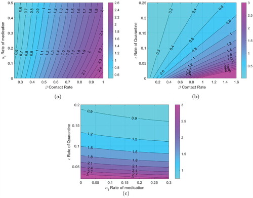
4.4. Variation of ${\mathcal{R}}_0$ with different control parameters

We would like to study how ${\mathcal{R}}_0$ changes with the parameters of the model, in particular we are interested in the variation of ${\mathcal{R}}_0$ as the quarantine rate, the contact rate and the rate of medication are varied. These rates can be changed by the use of different control strategies, this in turn will be used to project the epidemic curve under various control regimes.

In Figure 2(a), the contours of ${\mathcal{R}}_0$ are plotted against ${\alpha }_I$ the rate of medication and β the contact rate. In our analysis, we assume that the contact rate can be changed by following stricter social distancing protocols, the medication rate of course can be varied by wider use of available medication. We have also assumed that available medication reduced the duration of the disease by 25$\mathrm{\%}$, as reported in several studies. We note that while a higher medication rate (with this particular efficacy) reduces ${\mathcal{R}}_0$ medication by itself cannot make ${\mathcal{R}}_0<1$ for high contact rates. Figure 2(b) is a contour plot of ${\mathcal{R}}_0$ with quarantine rate (ε) and the contact rate (β). The primary mechanism of quarantine is lock down, although self-quarantine can also help. We note that ${\mathcal{R}}_0$ can be reduced significantly by either enforcing strict social distancing, thereby reducing β or by enforcing a lock down and reducing ε. In Figure 2(c), contours of ${\mathcal{R}}_0$ are plotted against the medication rate and the quarantine rate. We note again that while medication does lower the value of ${\mathcal{R}}_0$, for very low quarantine rates just using medication as a control strategy cannot make ${\mathcal{R}}_0<1$.

Figure 2. Contour comparison of ${\mathcal{R}}_0$. (a) Medication vs Contact rate. (b) Quarantine vs Contact rate. (c) Medication vs Quarantine.

5. Estimation and forecasting

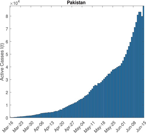
5.1. Data sources

The epidemic data of COVID-19 Pakistan for this study is sourced from the COVID-19 Data Repository by the Center for Systems Science and Engineering (CSSE) at Johns Hopkins University [12]. The epidemic data consist of three time series of confirmed cases, deaths and the recovered cases spanning over more than ten weeks till 15 June 2020, including the lock down period of 5 weeks. The active cases time series shown in Figure 3 is calculated as $I(t)=\mathrm{Confirmed}\mathrm{cases}-\mathrm{Deaths}-\mathrm{Recoverd}$

Figure 3. COVID-19 Epidemic data of Pakistan.

5.2. Estimation

The transmissibility of an infection is quantified by a threshold quantity ${\mathcal{R}}_0$, which is defined as average number of newly infected individuals by a single infected individual in complete susceptible population. For an ongoing epidemic of COVID-19, estimates of ${\mathcal{R}}_0$ can give better insights about the transmissibility of infection in a certain country. These estimates further depend upon the critical parameter such as contact rate β, incubation rate σ and other related parameters. Since there are control polices such as social distancing measures and quarantine being enforced in order to lessen effective contacts between susceptible and infected population groups. It is assumed that the effective contact rate is function of time. During lock down individuals will have less interaction as compared to after lock down so it is assumed to have two different contact rates of β, hence giving us a different transmissibility index. $\begin{array}{rl}\beta (t)& =\{\begin{array}{ll}{\beta }_{\mathrm{lockdown}}& t<t^{\ast }\\ {\beta }_{\mathrm{post}\mathrm{lockdown}}& t\ge t^{\ast }\end{array}\end{array}$ where $t^{\ast }$ is the time when lock down was relaxed. For Pakistan, the epidemic curve has followed two very different trajectories before and after the lock down was eased. As we have described in detail in the Introduction the strict lock down was relaxed around the beginning of the fourth week of April, hence $t^{\ast }$ is taken to be 5 weeks starting from 16 March 2020.

Since the direct estimates of parameters are really difficult especially, when epidemic/pandemic is still going on. However, we can adopt an indirect method proposed by the [7,8] to estimates these parameters from the infected data available. The ordinary least square (OLS) optimization technique is used which assumed that the observed data has the constant variance error distribution. $Y_j=f(t_j,{\mathrm{\Theta }}_{OLS})+{ϵ}_j$ where $Y_j$ are the observed values, ${\mathrm{\Theta }}_{OLS}$ are set of optimized parameters such as $\beta ,\gamma ,\sigma$ etc using standard OLS optimization (7(7) ${\mathrm{\Theta }}_{OLS}={\arg \min }_{\mathrm{\Theta }\in \mathrm{\Omega }}\sum _{j=1}^n[Y_j-f(t_j,\mathrm{\Theta }){]}^2$(7) ) And $f(\cdot )$ is nonlinear function associated with fitting model. In this case, the model (2(2) $\begin{array}{rl}\frac{\mathrm{d}S}{\mathrm{d}t}& =\mathrm{\Pi }+\xi Q_S-(\lambda +\mu +ϵ)S\\ \frac{\mathrm{d}{Q}_S}{\mathrm{d}t}& =ϵS-(\xi +\mu )Q_S\\ \frac{\mathrm{d}E}{\mathrm{d}t}& =\rho \lambda S-(\sigma +\mu )E\\ \frac{\mathrm{d}I}{\mathrm{d}t}& =\sigma E-({\delta }_I+\tau +{\alpha }_I+\mu +\gamma )I\\ \frac{\mathrm{d}A}{\mathrm{d}t}& =(1-\rho )\lambda S-({\theta }_A+\mu )A\\ \frac{\mathrm{d}{Q}_I}{\mathrm{d}t}& =\tau I-(\theta +{\alpha }_Q+{\delta }_Q+\mu )Q_I\\ \frac{\mathrm{d}M}{\mathrm{d}t}& ={\alpha }_{I}I+{\alpha }_Q{Q}_I-({\theta }_M+\mu )M\\ \frac{\mathrm{d}R}{\mathrm{d}t}& =\theta Q_I+\gamma I+{\theta }_{A}A+{\theta }_{M}M-\mu R\end{array}$(2) ) is the underlying model for fitting (Figure 4). (7) ${\mathrm{\Theta }}_{OLS}={\arg \min }_{\mathrm{\Theta }\in \mathrm{\Omega }}\sum _{j=1}^n[Y_j-f(t_j,\mathrm{\Theta }){]}^2$(7) We estimate different parameters of the model, specifically the contact rate β is estimated, this in turn is used to determine the value of ${\mathcal{R}}_0$ prior to and after the relaxation of the lock down. The values are given in Table 1.

Figure 4. Estimation of ${\mathcal{R}}_0$.

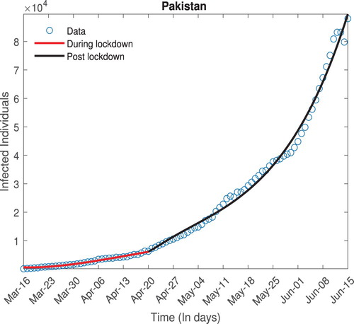
The value of ${\mathcal{R}}_0$ post-relaxation is significantly higher as can be expected, we will use this to project the epidemic curve under a variety of scenarios. We also note the significant reduction in the quarantine rate once the lock down was relaxed.

Table 1. Estimates of ${\mathcal{R}}_0$ for different epidemic phases.

Phase time	${\mathcal{R}}_0$	β	ε
During lock down	1.07	1.39	0.172
After lock down	1.8614	1.77	0.08

5.3. Forecasting

In this section, we project the epidemic curve under different quarantine, social distancing and medication strategies. At the moment, there is no government-mandated lock down in Pakistan; however, some people are observing self-quarantine measures, there are, however, guidelines for proper social distancing in public spaces, and as the infected numbers rise the health authorities are enforcing those guidelines, we consider this to essentially reduce the effective contact rate, finally medication has been approved by the government to treat COVID 19, and we hope that in the coming days it will become widely available. We consider three possible quarantine scenarios, the first where no additional steps are taken by the government, we call this the 'minimal quarantine', the second 'moderate quarantine', where some additional lock down measures are enforced to increase the quarantine rate to be twice of the post lock down value and finally a 'strict quarantine' where measures are taken to bring the quarantine rate back to the pre lock down levels. For each one of these cases we consider high, medium and low levels of social distancing leading to reduced effective contact rates, both with medication and without the availability of medication.

In Figure 5, we consider the scenario where no steps to lock down are taken and the quarantine rate remains at the post lock down level for different contact rates. Decreasing the contact rate not only lowers the peak of the epidemic curve but also shifts it to the left, which means that the disease will peak earlier. For the case when no medication is available Figure 5(a), we note that the peak will be reached in mid to late September with the maximum number of active infected being around 700, 000 for low levels of social distancing, 400, 000 for moderate social distancing and 200, 000 if high levels of social distancing are enforced. We also note that in these scenarios, the case-related fatalities that can be expected by December 2020 are, respectively, 2.5, 2 and 1.5 million. In Figure 5(b), for when medication is available we note that the disease peaks between August and early September and the maximum active infected number are now reduced to 275, 000, 150, 000 and 110, 000 in the three different social distancing scenarios. Around 1 million, 700, 000 and 450, 000 deaths can occur in these cases by the years end.

Figure 5. Forecasting with mild lock down. (a) Without medication. (b) With medication. (c) Without medication. (d) With medication.

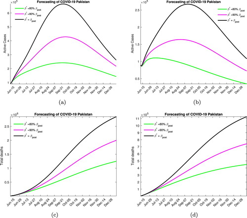
We would like to note that this is not a very likely scenario as the rising numbers of infected and disease-related deaths have prompted a response both in terms of some additional lock down measures and stricter implementation of the social distancing protocols.

In Figure 6, we consider the outcome when a moderate lock down is imposed increasing the quarantine rate to twice the post lock down level. Without medication Figure 6(a), we note that the peak will be reached in mid to late July if social distancing protocols are enforced and in mid to late August otherwise, the maximum number of active infected in these cases is projected to be around 150, 000, 175, 000 and 300, 000. The total expected fatalities due to disease are around 500, 000, 800, 000 and 1.2 million, respectively, through December. In Figure 6(b), for the case medication, we note that disease peaks between early to mid-July and the maximum active infected number with a high level of social distancing is around 100, 000, with disease-related fatalities through December projected to be around 225, 000. With moderate social distancing, the maximum infected number is projected to be 120, 000 with 325, 000 expected deaths by the end of the year. Finally, with low social distancing efforts, we expect 150, 000 active infected cases at the peak of the outbreak and 500, 000 total fatalities.

Figure 6. Forecasting with moderate lock down. (a) Without medication. (b) With medication. (c) Without medication. (d) With medication.

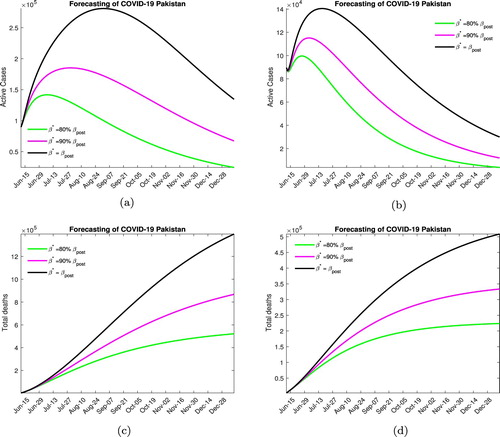
In our opinion, the most likely scenario to be played out over the next few month will involve moderate lock down and high social distancing efforts.

In Figure 7, we consider the situation when a strict lock down is imposed increasing the quarantine rate to pre-lock down level. Without medication, Figure 7(a), the peak will be reached in early to mid July (depending on the contact rate) with the maximum number of active infected being around 125, 000−200, 000. In this scenario, 300, 000−700, 000 disease-related deaths are expected by the end of the year. In Figure 7(b), when medication is available, the disease peaks between late June to early July with the maximum active infected number being around 90, 000−125, 000 (again depending on the social distancing measures), with around 150, 000−300, 000 deaths due the the infection.

Figure 7. Forecasting with strict lock down. (a) Without medication. (b) With medication. (c) Without medication. (d) With medication.

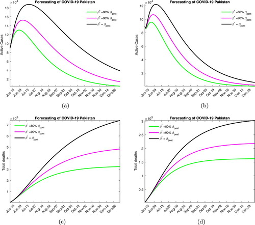
We would like to point out that this level of quarantine is not very realistic, considering the economic and social costs the government is unlikely to enforce such stringent lock down measures.

6. Conclusion

In this study, we have estimated the severity of the COVID 19 outbreak in Pakistan, modelling the transmission dynamics of the disease using an extension of the SEIR model. The model includes important transmission pathways such as asymptomatics, quarantined and isolated individuals as well as the medicated population subgroup. We also use this model to project the epidemic curve and give estimates of the disease burden under various realistic control strategies.

An ordinary differential equation-based model is used for the transmission dynamic of COVID 19 as described by (2(2) $\begin{array}{rl}\frac{\mathrm{d}S}{\mathrm{d}t}& =\mathrm{\Pi }+\xi Q_S-(\lambda +\mu +ϵ)S\\ \frac{\mathrm{d}{Q}_S}{\mathrm{d}t}& =ϵS-(\xi +\mu )Q_S\\ \frac{\mathrm{d}E}{\mathrm{d}t}& =\rho \lambda S-(\sigma +\mu )E\\ \frac{\mathrm{d}I}{\mathrm{d}t}& =\sigma E-({\delta }_I+\tau +{\alpha }_I+\mu +\gamma )I\\ \frac{\mathrm{d}A}{\mathrm{d}t}& =(1-\rho )\lambda S-({\theta }_A+\mu )A\\ \frac{\mathrm{d}{Q}_I}{\mathrm{d}t}& =\tau I-(\theta +{\alpha }_Q+{\delta }_Q+\mu )Q_I\\ \frac{\mathrm{d}M}{\mathrm{d}t}& ={\alpha }_{I}I+{\alpha }_Q{Q}_I-({\theta }_M+\mu )M\\ \frac{\mathrm{d}R}{\mathrm{d}t}& =\theta Q_I+\gamma I+{\theta }_{A}A+{\theta }_{M}M-\mu R\end{array}$(2) ). DFE and an endemic equilibrium when the disease is endemic in the population are derived. We establish a threshold quantity ${\mathcal{R}}_0$ in terms of the parameters of the model, observing that the disease dies out whenever ${\mathcal{R}}_0<1$ and is endemic if ${\mathcal{R}}_0>1$. We study the variation of ${\mathcal{R}}_0$ on some of the model parameters, specifically on the parameters which can be varied by various control mechanisms, such as quarantine, social distancing and medication. We note that quarantine and social distancing and medication can help in lowering the value of ${\mathcal{R}}_0$ and bring the epidemic under control, with quarantine being the most effective mechanism followed by social distancing and medication. However there are practical difficulties in establishing a strict quarantine as is evident from the relaxation of lock downs in most countries, hence a mix of all these strategies is perhaps the best way forward.

Noting that in Pakistan the epidemic progressed in two distinct phases, before and after the lock down restrictions were relaxed, we estimate the value of ${\mathcal{R}}_0$ separately for both these phases. For the pre-relaxation phase we estimate ${\mathcal{R}}_0=1.07$ and for the post-relaxation phase our estimate comes out to be ${\mathcal{R}}_0=1.86$. This is consistent with the growth dynamics and other estimates in the literature.

These results are then used to project the epidemic curve. We explore various possible scenarios, with varying levels of lock down, social distancing and medication. The lock down and social distancing measures are captured by quarantine rate (ε) and contact rate (β) in our study. In the case where a strict lock down is enforced taking the quarantine rate back to pre-relaxation level, varying the contact and medication rates, we observe that in the best case scenario with high level of all controls the epidemic will peak around late June to early July with a maximum active infected number around 90, 000. For a moderate lock down which is modelled by taking the quarantine rate to be twice the post-relaxation rate, and varying the contact and medication rates we note that the epidemic will peak around mid July with the active infected numbers around 120, 000 at that point considering that social distancing measures are enhanced. Finally, we look at the case when no further lock down measures are taken and the quarantine rate remains at the value estimated on June 15, in this scenario, we note that the epidemic will peak around late September with the maximum active infected number around 700, 000.

In this work, we estimated the severity of the COVID 19 outbreak in Pakistan, noting that the epidemic followed two different trajectories before and after lock down restrictions were relaxed. The restrictions we observe kept the value of ${\mathcal{R}}_0$ close to 1 ; however, once the restrictions were eased the number of cases increased at a high rate, reflected in ${\mathcal{R}}_0=1.86$. We also generated possible future trajectories based on intervention and control measures to varying degrees. In case no significant measures are taken at the peak of the epidemic, which will occur in September the maximum active cases will cross the 700, 000 mark while in a very optimistic scenario this will happen in early July with maximum active cases contained to around 150, 000. We strongly agree with the recent WHO recommendation that some form of moderate lock down needs to be reinforced. This along with social distancing and possible medication will result in a disease peak sometime in mid-July and contain the maximum active infected numbers to around 120, 000. Inaction at this point of the epidemic is projected to have very serious consequences both in terms of disease burden and mortality.

Disclosure statement

No potential conflict of interest was reported by the author(s).

Data availability statement

The data that support the findings of this study are openly available in at COVID-19 Data Repository by the Center for Systems Science and Engineering (CSSE) at Johns Hopkins University [12https://github.com/CSSEGISandData/COVID-19, reference number].

Appendix

A.1. Proof of Lemma 3.1

Proof.

To show $\mathcal{B}$ is positive invariant, we need to show first that all state variables with non-negative initial conditions remain nonnegative for $t\ge 0$ and second that $N(0)\le \frac{\mathrm{\Pi }}{\mu }$ implies $N(t)\le \frac{\mathrm{\Pi }}{\mu }$ for all $t\ge 0$.

1. Non-negativity of solutions

   We used a similar approach (Theorem 2.1 of [24]) to prove positivity of solutions.

   Let $t_1=sup\{t>0:S>0,Q_S>0,E>0,I>0,A>0,Q_I>0,M>0,R>0\in [0,t]\}$, thus $t_1>0$. It follows from the first equation of (2(2) $\begin{array}{rl}\frac{\mathrm{d}S}{\mathrm{d}t}& =\mathrm{\Pi }+\xi Q_S-(\lambda +\mu +ϵ)S\\ \frac{\mathrm{d}{Q}_S}{\mathrm{d}t}& =ϵS-(\xi +\mu )Q_S\\ \frac{\mathrm{d}E}{\mathrm{d}t}& =\rho \lambda S-(\sigma +\mu )E\\ \frac{\mathrm{d}I}{\mathrm{d}t}& =\sigma E-({\delta }_I+\tau +{\alpha }_I+\mu +\gamma )I\\ \frac{\mathrm{d}A}{\mathrm{d}t}& =(1-\rho )\lambda S-({\theta }_A+\mu )A\\ \frac{\mathrm{d}{Q}_I}{\mathrm{d}t}& =\tau I-(\theta +{\alpha }_Q+{\delta }_Q+\mu )Q_I\\ \frac{\mathrm{d}M}{\mathrm{d}t}& ={\alpha }_{I}I+{\alpha }_Q{Q}_I-({\theta }_M+\mu )M\\ \frac{\mathrm{d}R}{\mathrm{d}t}& =\theta Q_I+\gamma I+{\theta }_{A}A+{\theta }_{M}M-\mu R\end{array}$(2) ) that

   Table A1. Description of the variables of the model (2(2) $\begin{array}{rl}\frac{\mathrm{d}S}{\mathrm{d}t}& =\mathrm{\Pi }+\xi Q_S-(\lambda +\mu +ϵ)S\\ \frac{\mathrm{d}{Q}_S}{\mathrm{d}t}& =ϵS-(\xi +\mu )Q_S\\ \frac{\mathrm{d}E}{\mathrm{d}t}& =\rho \lambda S-(\sigma +\mu )E\\ \frac{\mathrm{d}I}{\mathrm{d}t}& =\sigma E-({\delta }_I+\tau +{\alpha }_I+\mu +\gamma )I\\ \frac{\mathrm{d}A}{\mathrm{d}t}& =(1-\rho )\lambda S-({\theta }_A+\mu )A\\ \frac{\mathrm{d}{Q}_I}{\mathrm{d}t}& =\tau I-(\theta +{\alpha }_Q+{\delta }_Q+\mu )Q_I\\ \frac{\mathrm{d}M}{\mathrm{d}t}& ={\alpha }_{I}I+{\alpha }_Q{Q}_I-({\theta }_M+\mu )M\\ \frac{\mathrm{d}R}{\mathrm{d}t}& =\theta Q_I+\gamma I+{\theta }_{A}A+{\theta }_{M}M-\mu R\end{array}$(2) ).

   Variable	Description
   N	Total population
   S	Susceptible individuals
   $Q_S$	Quarantine of susceptible individuals
   E	Individuals exposed to corona virus
   I	Individuals infected with corona virus
   A	Asymptomatic individuals
   $Q_I$	Isolated individuals
   M	Medication of individuals
   R	Recovered from corona virus

   Table A2. Description of the parameters of the model.

   Parameters	Description	Values
   Π	Recruitment rate of humans	100	Assumed
   μ	Natural death rate of humans	60 years	Assumed
   ${\delta }_I$	Disease-induced death rate individuals	$0.02{\mathrm{day}}^{-1}$	Estimated from data
   ${\delta }_Q$	Disease-induced death rate of isolated individuals	$0.02{\mathrm{day}}^{-1}$	Estimated from data
   $\frac{1}{\sigma }$	Incubation rate of susceptible individuals	12 days	Estimated from data
   $\frac{1}{\gamma }$	Recovery rate of infected individuals	4 days	[9,10]
   β	Effective contact rate	1.7	Estimated from data
   ρ	Probability of getting exposed to covid-19	$70\mathrm{\%}=0.7$	Estimated from data
   τ	Isolation rate of infected individuals	0.1	[9]
   ${\alpha }_I$	medication rate of infected individuals	0.1	Assumed
   ${\theta }_A$	Recovery rate of Asymptomatic individuals	$0.1$	Estimated from data
   θ	Recovery rate of Isolated individuals	$0.1875$	[9,10]
   ${\theta }_M$	Recovery rate of medicated individuals	$0.375$	Assumed
   ε	susceptible Quarantine rate of Susceptible individuals	$0.08$	Estimated from data
   ξ	Waning rate of susceptible quarantined individuals to susceptible class	28 Days	Assumed
   ${\eta }_1$	Modification parameter for relative infectiousness of Isolated individuals	$0.4$	Assumed
   ${\eta }_2$	Modification parameter for relative infectiousness of asymptomatic individuals	$0.5$	[9]
   ${\eta }_4$	Modification parameter for relative infectiousness of medication	$0.5$	Assumed

   $\begin{array}{rl}{\displaystyle \frac{\mathrm{d}S}{\mathrm{d}t}}& =\mathrm{\Pi }+\xi Q_S-(\lambda +\mu +ϵ)S\ge \mathrm{\Pi }-(\lambda +\mu +ϵ)S\\ {\displaystyle \frac{\mathrm{d}S}{\mathrm{d}t}}& \ge \mathrm{\Pi }-(\lambda +\mu +ϵ)S\end{array}$ which we can re-write with the help of integrating factor ${\displaystyle \frac{\mathrm{d}}{\mathrm{d}t}}(S\exp [\mu t+ϵt+{\int }_0^t\lambda (\tau )\mathrm{d}\tau ])\ge \mathrm{\Pi }\exp [\mu t+ϵt+{\int }_0^t\lambda (\tau )\mathrm{d}\tau ]$ Integrating from 0 to $t_1$ $\begin{array}{rl}& ⟹S(t_1)\exp [\mu t_1+ϵt_1+{\int }_0^{t_1}\lambda (\tau )\mathrm{d}\tau ]-S(0)\\ & \ge {\int }_0^{t_1}(\mathrm{\Pi }\exp [\mu z+ϵz+{\int }_0^z\lambda (\tau )d\tau ])\mathrm{d}z\end{array}$ So that $\begin{array}{rl}S(t)& \ge \exp [-\mu t_1-ϵt_1-{\int }_0^{t_1}\lambda (\tau )\mathrm{d}\tau ]\\ & \times \{S(0)+{\int }_0^{t_1}(\mathrm{\Pi }\exp [\mu z+ϵz+{\int }_0^z\lambda (\tau )\mathrm{d}\tau ])\mathrm{d}z\}>0\end{array}$ for all $t>0$. Similarly, we can establish the results for $Q_S>0,E>0,I>0,A>0,Q_I>0,M>0$, and R>0. The non-negativity can also be shown using methods in the Appendix of [26].

2. $N(0)\le {\displaystyle \frac{\mathrm{\Pi }}{\mu }}⟹N(t)\le {\displaystyle \frac{\mathrm{\Pi }}{\mu }}\mathrm{for}\mathrm{all}t\ge 0$Adding the equations of model (2(2) $\begin{array}{rl}\frac{\mathrm{d}S}{\mathrm{d}t}& =\mathrm{\Pi }+\xi Q_S-(\lambda +\mu +ϵ)S\\ \frac{\mathrm{d}{Q}_S}{\mathrm{d}t}& =ϵS-(\xi +\mu )Q_S\\ \frac{\mathrm{d}E}{\mathrm{d}t}& =\rho \lambda S-(\sigma +\mu )E\\ \frac{\mathrm{d}I}{\mathrm{d}t}& =\sigma E-({\delta }_I+\tau +{\alpha }_I+\mu +\gamma )I\\ \frac{\mathrm{d}A}{\mathrm{d}t}& =(1-\rho )\lambda S-({\theta }_A+\mu )A\\ \frac{\mathrm{d}{Q}_I}{\mathrm{d}t}& =\tau I-(\theta +{\alpha }_Q+{\delta }_Q+\mu )Q_I\\ \frac{\mathrm{d}M}{\mathrm{d}t}& ={\alpha }_{I}I+{\alpha }_Q{Q}_I-({\theta }_M+\mu )M\\ \frac{\mathrm{d}R}{\mathrm{d}t}& =\theta Q_I+\gamma I+{\theta }_{A}A+{\theta }_{M}M-\mu R\end{array}$(2) ), this results in change in total population as (A1) $\frac{\mathrm{d}N}{\mathrm{d}t}=\mathrm{\Pi }-\mu N-({\delta }_{I}I+{\delta }_Q{Q}_I)$(A1) Assuming positive initial conditions, we know from (a) that I and $Q_I$ remain positive for $t\ge 0$ and therefore (A2) $\frac{\mathrm{d}N}{\mathrm{d}t}\le \mathrm{\Pi }-\mu N$(A2) It follows that (by use of an integrating factor) (A3) $N(t)\le N(0)e^{-\mu t}+\frac{\pi }{\mu }(1-e^{-\mu t})$(A3) for $t\ge 0$ which, together with $N(0)\le \frac{\mathrm{\Pi }}{\mu }$, implies $N(t)\le \frac{\mathrm{\Pi }}{\mu }$ for all $t>0$.

References

- M. Ali, I. Mudassar, and K. Adnan, COVID-19: can medication mitigate the need for a strict lock down? Lett. Biomath. (2020 July). Available at https://lettersinbiomath.journals.publicknowledgeproject.org/index.php/lib/article/view/365.
- M. Ali, S. Shah, M. Imran, and A. Khan, The role of asymptomatic class, quarantine and isolation in the transmission of COVID-19, J. Biol. Dynam. 14(1) (2020), pp. 389–408. doi: 10.1080/17513758.2020.1773000
- H.I. Aslan, Modeling COVID-19: Forecasting and analyzing the dynamics of the outbreak in Hubei and Turkey. Preprint Available at https://doi.org/10.1101/2020.04.11.20061952.
- J. Beigel, K. Tomashek, L. Dodd, A. Mehta, B. Zingman, A. Kalil, E. Hohmann, H. Chu, A.Luetkemeyer, S. Kline, D. Lopez de Castilla, R. Finberg, K. Dierberg, V. Tapson, L. Hsieh, T. Patterson, R. Paredes, D. Sweeney, W. Short, G. Touloumi, D. Lye, N. Ohmagari, M. Oh, G. Ruiz-Palacios, T. Benfield, G. Fätkenheuer, M. Kortepeter, R. Atmar, C. Creech, J. Lundgren, A. Babiker, S.Pett, J. Neaton, T. Burgess, T. Bonnett, M. Green, M. Makowski, A. Osinusi, S. Nayak, and H. Lane, Remdesivir for the treatment of Covid-19 – preliminary report, N. Engl. J. Med. (2020). Available at https://doi.org/10.1056/NEJMoa2007764.
- Centers for Disease Control and Prevention, Coronavirus disease 2019 (COVID-19). [online] Available at: https://www.cdc.gov/coronavirus/2019-ncov/ [Accessed 25 April 2020]. 2020.
- T. Chen, J. Rui, Q. Wang, Z. Zhao, J. Cui, and L. Yin, A mathematical model for simulating the phase-based transmissibility of a novel coronavirus, Infect. Dis. Poverty 9(1) (2020). Available at https://doi.org/10.1186/s40249-020-00640-3.
- A. Cintrón-Arias, C. Castillo-Chávez, L.M.A. Bettencourt, A.L. Lloyd, and H.T. Banks, The estimation of the effective reproductive number from disease outbreak data, Math. Biosci. Eng. 6 (2009), pp. 261–282. Available at https://doi.org/10.3934/mbe.2009.6.261.
- B. Efron and R.J. Tibshirani, An Introduction to The Bootstrap, Chapman & Hall/CRC, Boca Raton, FL, 1993.
- S. Eikenberry, M. Mancuso, E. Iboi, T. Phan, K. Eikenberry, Y. Kuang, E. Kostelich, and A. Gumel, To mask or not to mask: modeling the potential for face mask use by the general public to curtail the COVID-19 pandemic, Infect Dis Model. 5 (2020), pp. 293–308.
- N. Ferguson, D. Laydon, G. Nedjati Gilani, N. Imai, K. Ainslie, M. Baguelin, S. Bhatia, A. Boonyasiri, Z. Cucunuba Perez, G. Cuomo-Dannenburg, A. Dighe, I. Dorigatti, H. Fu, K. Gaythorpe, W. Green, A. Hamlet, W. Hinsley, L. Okell, S. Van Elsland, H. Thompson, R. Verity, E. Volz, H. Wang, Y.Wang, P. Walker, C. Walters, P. Winskill, C. Whittaker, C. Donnelly, S. Riley, and A. Ghani, Report 9: impact of non-pharmaceutical interventions (Npis) to reduce COVID19 mortality and healthcare demand. [online] Hdl.handle.net. Available at: http://hdl.handle.net/10044/1/77482 [Accessed 2 May 2020], 2020.
- Gilead.com, COVID-19. [online] Available at: https://www.gilead.com/purpose/advancing-global-health/covid-19. 2020.
- GitHub, Cssegisanddata/COVID-19. [online] Available at: https://github.com/CSSEGISandData/COVID-19 [Accessed 15 June 2020], 2020.
- J. Grein, N. Ohmagari, D. Shin, Compassionate use of remdesivir for patients with severe Covid-19. N. Engl. J. Med.no. 382(24)) (2020), pp. 2327–2336. https://doi.org/10.1056/NEJMoa2007016.
- B. Hu, X. Ge, L. Wang, and Z. Shi, Bat origin of human coronaviruses, Virol. J. 12(1) (2015). Available at: https://doi.org/10.1186/s12985-015-0422-1.
- C. Huang, Y. Wang, X. Li, L. Ren, J. Zhao, Y. Hu, L. Zhang, G. Fan, J. Xu, X. Gu, Z. Cheng, T.Yu, J. Xia, Y. Wei, W. Wu, X. Xie, W. Yin, H. Li, M. Liu, Y. Xiao, H. Gao, L. Guo, J. Xie, G. Wang, R. Jiang, Z. Gao, Q. Jin, J. Wang, and B. Cao, Clinical features of patients infected with 2019 novel coronavirus in wuhan, China, Lancet 395 (2020), pp. 497–506. doi: 10.1016/S0140-6736(20)30183-5
- I. Hung, K. Lung, E. Tso, R. Liu, T. Chung, M. Chu, Y. Ng, J. Lo, J. Chan, A. Tam, H. Shum, V.Chan, A. Wu, K. Sin, W. Leung, W. Law, D. Lung, S. Sin, P. Yeung, C. Yip, R. Zhang, A. Fung, E. Yan, K. Leung, J. Ip, A. Chu, W. Chan, A. Ng, R. Lee, K. Fung, A. Yeung, T. Wu, J. Chan, W.Yan, W. Chan, J. Chan, A. Lie, O. Tsang, V. Cheng, T. Que, C. Lau, K. Chan, K. To, and K. Yuen, Triple combination of interferon beta-1b, lopinavir–ritonavir, and ribavirin in the treatment of patients admitted to hospital with COVID-19: an open-label, randomised, phase 2 trial, Lancet 395 (2020), pp. 1695–1704. doi: 10.1016/S0140-6736(20)31042-4
- A. Kucharski, T. Russell, and C. Diamond, Early dynamics of transmission and control of COVID-19: a mathematical modelling study, Lancet Infect Dis (2020). Available at https://doi.org/10.1016/s1473-3099(20)30144-4.
- Q. Lin, S. Zhao, D. Gao, Y. Lou, S. Yang, S. S. Musa, M. H. Wang, Y. Cai, W. Wang, L. Yang, and D. He, A conceptual model for the coronavirus disease 2019 (COVID-19) outbreak in Wuhan, China with individual reaction and governmental action, Int. J. Infect. Dis. 93 (2020), pp. 211–216. Available at https://doi.org/10.1016/j.ijid.2020.02.058.
- M. Nicola, Z. Alsafi, C. Sohrabi, A. Kerwan, A. Al-Jabir, C. Iosifidis, M. Agha, and R. Agha, The socio-economic implications of the coronavirus and COVID-19 pandemic: a review, Int. J. Surg. 78 (2020), pp.185–193. Available at https://doi.org/10.1016/j.ijsu.2020.04.018.
- Q. Nimubona, C. Smith, A. Mackinnon, W. Braw, Zenko, A coronavirus mystery: why are there so few cases In South Asia? [online] Foreign Policy. Available at: https://foreignpolicy.com/2020/04/30/coronavirus-mystery-why-so-few-cases-south-asia-india-pandemic-lockdown. 2020.
- Oie.int, Questions and answers on the COVID-19: OIE – World Organisation For Animal Health. [online] Available at: https://www.oie.int/scientific-expertise/specific-information-and-recommendations/questions-and-answers-on-2019novel-coronavirus [Accessed 25 April 2020]. 2020.
- L. Pang, S. Liu, X. Zhang, T. Tian, and Z. Zhao, Transission dynamics and control strategies of COVID-19 in Wihan China, J. Biol. Syst. (92020), pp. 1–18. doi: 10.1142/S0218339020500096
- A. Perkins and G. Espana, Optimal control of the COVID-19 pandemic with non-pharmaceutical interventions. (Preprint) 2020. Available at https://doi.org/10.1101/2020.04.22.20076018.
- M.A. Safi and A.B. Gumel, Global asymptotic dynamics of a model for quarantine and isolation, Discrete & Continuous Dynam. Syst. – B 14(1) (2010), pp. 209–231. doi: 10.3934/dcdsb.2010.14.209
- E. Sallard, F. Lescure, Y. Yazdanpanah, F. Mentre, and N. Peiffer-Smadja, Type 1 interferons as a potential treatment against COVID-19, Antiviral Res. 178 (2020), p. 104791. doi: 10.1016/j.antiviral.2020.104791
- H.R. Thieme, Mathematics in Population Biology, Princeton University Press, OXFORD, 2003.https://doi.org/10.2307/j.ctv301f9v.
- P. van den Driessche and J. Watmough, Reproduction numbers and sub-threshold endemic equilibria for compartmental models of disease transmission, Math. Biosci. 180 (2002), pp. 29–48. doi: 10.1016/S0025-5564(02)00108-6
- Who.int, Accelerating a safe and effective COVID-19 vaccine. [online] Available at: https://www.who.int/emergencies/diseases/novel-coronavirus-2019/global-research-on-novel-coronavirus-2019-ncov/accelerating-a-safe-and-effective-covid-19-vaccine. 2020.
- Who.int, Solidarity clinical trial for COVID-19 treatments. [online] Available at: https://www.who.int/emergencies/diseases/novel-coronavirus-2019/global-research-on-novel-coronavirus-2019-ncov/solidarity-clinical-trial-for-covid-19-treatments. 2020.
- Who.int, Coronavirus. [online] Available at: https://www.who.int/health-topics/coronavirus [Accessed 25 April 2020]. 2020.
- Worldometers.info, Coronavirus Update (Live): 2,874,022 Cases And 200,790 Deaths From COVID-19 Virus Pandemic – Worldometer. [online] Available at: https://www.worldometers.info/coronavirus/ [Accessed 25 April 2020]. 2020.
- J. Yang, Y. Zheng, X. Gou, K. Pu, Z. Chen, Q. Guo, R. Ji, H. Wang, Y. Wang, and Y. Zhou, Prevalence of comorbidities and its effects in coronavirus disease 2019 patient: a systematic review and meta-analysis, Int. J. Infect. Dis. 94 (2020), pp. 91–95. doi: 10.1016/j.ijid.2020.03.017
- S. Zhao, Q. Lin, J. Ran, S. S. Musa, G. Yang, W. Wang, Y. Lou, D. Gao, L. Yang, D. He, and M. H.Wang, Preliminary estimation of the basic reproduction number of novel coronavirus (2019-nCoV) in China, from 2019 to 2020: a data-driven analysis in the early phase of the outbreak, Int. J. Infect. Dis.92 (2020), pp. 214–217. Available at https://doi.org/10.1016/j.ijid.2020.01.050.