A bifurcation theorem for Darwinian matrix models and an application to the evolution of reproductive life-history strategies

Abstract

We prove bifurcation theorems for evolutionary game theoretic (Darwinian dynamic) versions of nonlinear matrix equations for structured population dynamics. These theorems generalize existing theorems concerning the bifurcation and stability of equilibrium solutions when an extinction equilibrium destabilizes by allowing for the general appearance of the bifurcation parameter. We apply the theorems to a Darwinian model designed to investigate the evolutionary selection of reproductive strategies that involve either low or high post-reproductive survival (semelparity or iteroparity). The model incorporates the phenotypic trait dependence of two features: population density effects on fertility and a trade-off between inherent fertility and post-reproductive survival. Our analysis of the model determines conditions under which evolution selects for low or for high reproductive survival. In some cases (notably an Allee component effect on newborn survival), the model predicts multiple attractor scenarios in which low or high reproductive survival is initial condition dependent.

Keywords:

• Population dynamics
• evolutionary dynamics
• bifurcation
• equilibrium
• stability
• semelparity
• evolutionary stable strategies

AMS Subject Classifications:

• 92D15
• 39A11
• 37G35

1. Introduction

Individual life-history traits or strategies affecting survival and reproduction, and how they affect population level dynamics and basic issues such as population survival or extinction, play a prominent role in life-history theory [21,29,33]. The question of why organisms adopt one strategy over another is a very old question that traces its roots back to Aristotle and Linnaeus [23]. In an influential paper from last century, L. Cole [6] focussed on the strategies of semelparity and iteroparity. Individuals in a semelparous population do not survive reproduction whereas those in an iteroparous populations have multiple reproductive episodes. Cole concluded that evolution should favour a semelparous strategy, a conclusion that became known as ‘Cole's Paradox’ since iteroparous populations are ubiquitous in nature. Numerous mechanisms were explored in response to this paradox and have been offered to account for the evolution of these reproductive strategies, including juvenile survival [8,31]; density dependence [1,5,18,22,34,35]; bet-hedging against environmental stochasticity [3,4,18,33,36,37,41], and many others [19,29,30,33].

Central to life-history theory are trade-offs [21,29]. Trade-offs are often viewed as an allocation issue, specifically the allocation of food or energy resources to metabolism growth, or reproduction, etc. For example, resources allocated to fertility are not available to apply towards post-reproductive survival and vice versa, in which case fertility and post-reproductive survival are negatively correlated.

Further complications are that the binary descriptions of semelparity and iteroparity are often not suitable for many populations and circumstances. Hughes [23] argues in favour of a ‘continuum of modes of parity’, so that all individuals in a population may not have the same life-history traits or have plasticity with regard to traits that are affected by environmental circumstances. With this point of view in mind, our goal here is to derive and analyse some evolutionary game theoretic models in which fertility and survival depend on continuous phenotypic traits that are subject to the Darwinian evolution and, using example models, to investigate the evolutionary stability or instability of different life-history strategies. We will focus on the trait dependence of two key features: population density effects on fertility and a trade-off between inherent fertility and post-reproductive survival. In addition to the standard negative effects of population density on fertility and/or survival, our model allows for positive effects on newborn survival (Allee component effects [7]).

In Section 2, we derive a discrete time Darwinian model for dynamics of a population and a mean phenotypic trait on which fertility, survival, and density effects depend. In Section 4, we analyse the equilibrium and stability properties of the model using some theorems proved in Section 3 concerning equilibrium existence and stability for a general Darwinian model. The results in that section extend the local bifurcation and stability results for non-evolutionary model equations for the dynamics of structured populations found in [16] to an evolutionary setting. They also generalize the results for the Darwinian, structured population dynamic models studied in [10,17] and [28] by allowing for a more general bifurcation parameter μ. In these earlier results, either a linearly appearing parameter or the inherent population growth rate (which does not appear explicitly as a model parameter) is used as the bifurcation parameter, both of which constrain the applicability of these otherwise general theorems. Our results in Section 3 allow the use of any model parameter as a bifurcation parameter. In Section 4, we apply these theorems to the model derived in Section 2 and, in addition, supplement the analysis with some numerical simulation studies. The biological punch lines obtained from this analysis are discussed in Section 5.

2. A discrete-time Darwinian model with a fertility-survival trade-off

Let $x(t)$ denote the density of a population, at times $t=0,1,2,,3,\dots$, subject only to birth and death processes and in the absence of immigration or emigration. We take the unit of time to be an individual's maturation period and build a population dynamic model by accounting for the population at time t + 1 by only two means: newborns (individuals not present at time t) and those reproducing individuals at time t that survive to time t + 1. We assume that an individual's fertility is dependent upon available resources which are allocated between the production of newborns and processes that promote post-reproductive survival. Let f denote the fraction allocated to reproduction ($0\le f\le 1$), b>0 denote the per capita production of newborns per unit resource (per unit time), and let $s_n$ ($0<s_n\le 1$) denote the probability that a newborn born at time t survives to the next census $t+1.$ Then the density of newborns at time t + 1 equals $bf{s}_{n}x(t)$. In this model, we will assume that the fertility/survival trade-off is described by a probability of post-reproductive survival given by the formula $s_a(1-f)$ where $s_a$ ($0\le s_a\le 1$) is the maximal possible survival probability. Then $x(t+1)=bf{s}_{n}x(t)+s_a(1-f)x(t)$ or $x(t+1)=rx(t)$ where $r:=fb{s}_n+(1-f)s_a$is the population growth rate.

In addition to the fertility/survival trade-off, we want to study the effects that population density has on fertility and survival. We do this by introducing density factors into the growth rate (1) $r(x):=fb\beta (x)s_n\alpha (x)+(1-f)s_a\gamma (x)$(1) where β, α and γ describe the effects that population density has on fertility, newborn survival, and post-reproductive survival, respectively. We assume

H1: β, α and $\gamma \in C^2({\mathrm{\Omega }}^1,{\overline{R}}_{+}^1)$  satisfy $\beta (0)=\alpha (0)=\gamma (0)=1$, $s_n\alpha (x)\le 1$ and $s_a\gamma (x)\le 1.$

Here ${\overline{R}}_{+}^1$ is the set of nonnegative real numbers and ${\mathrm{\Omega }}^1$ is an open interval of real numbers that contains ${\overline{R}}_{+}^1$. The reason for the normalizations at x = 0 is so that b, $s_n$ and $s_a$ retain their biological interpretations as inherent rates (i.e. rates in the absence of density effects).

A familiar factor used throughout the literature to describe negative density effects (i.e. a decreasing function of x>0) is (2) $\frac{1}{1+cx}\mathrm{with}c>0.$(2) We refer to the coefficient c as the intraspecific competition coefficient since it accounts for the effect on an individual's fertility due to the presence of other individuals in the population (due, say, to competition for resources). We are also interested here in possible positive density effects (at least a low densities), which are called component Allee effects. Many mathematical expressions for such a factor can be found throughout the recent literature. In Section 4.2, we use (3) $\frac{1+\rho a{x}^q}{1+a{x}^q}\mathrm{with}q\ge 1,a\ge 0\mathrm{and}\rho >1$(3) for this purpose. (This expression seems to have been first introduced into population models by Jacobs [24].)

The scalar difference equation (4) $x(t+1)=r(x\left(t\right))x\left(t\right),$(4) together with (1(1) $r(x):=fb\beta (x)s_n\alpha (x)+(1-f)s_a\gamma (x)$(1) ), represents a general model for the dynamics of a population with the fertility versus survival trade-off and density-dependent features described above. Note that if all resource allocation goes towards reproduction, i.e. $f=1,$ then post-reproductive survival equals 0. In this case, the population is strictly semelparous in that no individual survives reproduction. We added the adjective ‘strictly’ since a population whose individuals have a very small post-reproductive survival rate could, for all practical purposes, still be considered semelparous. Only if f is significantly larger that 0 would the population be clearly designated as iteroparous, the cut-off point being subjectively chosen by the modeller. See [23] for a treatment of the difficulties with the binary classification of semelparity and iteroparity. Whatever language is used, we consider the fraction f in the model (4(4) $x(t+1)=r(x\left(t\right))x\left(t\right),$(4) )–(1(1) $r(x):=fb\beta (x)s_n\alpha (x)+(1-f)s_a\gamma (x)$(1) ) to be a basic life-history strategy, measuring the fraction of resources allocated to fertility versus post-reproductive survival.

To introduce evolutionary changes in the components of the model (4(4) $x(t+1)=r(x\left(t\right))x\left(t\right),$(4) )–(1(1) $r(x):=fb\beta (x)s_n\alpha (x)+(1-f)s_a\gamma (x)$(1) ) by means of evolutionary game theory, we consider the components in the per capita growth rate r to be associated with an individual in the population, at least one of which depends on a quantified phenotypic trait v of the individual. In this methodology, it is assumed the trait v is, at all times, normally distributed throughout the population with a constant variance. It follows that the trait distribution is determined by the population mean trait u. We allow model coefficients in r to depend on both the trait v of the individual and, in order to capture the influence of other individuals, on the population mean trait u. Thus, we write $r=r(x,u,v)$. Evolutionary game theory describes the coupled dynamics of x and u by the Darwinian equations [27,40](5) $\begin{array}{rl}x(t+1)& ={r(x\left(t\right),u\left(t\right),v)|}_{v=u\left(t\right)}x\left(t\right)\end{array}$(5) (6) $\begin{array}{rl}u(t+1)& =u\left(t\right)+{\sigma }^2{\frac{\mathrm{\partial }\ln r(x\left(t\right),u\left(t\right),v)}{\mathrm{\partial }v}|}_{v=u\left(t\right)}.\end{array}$(6) Here $\ln r$ is taken to be the measure of population fitness. The coefficient ${\sigma }^2\ge 0$ is the speed of evolution (it is proportional to the assumed constant variance of the trait throughout the population). If ${\sigma }^2=0$ (there is no trait variability), then $u(t)=u_0$ remains constant (i.e. there is no evolution) and the Darwinian equations reduce to the population Equation (4(4) $x(t+1)=r(x\left(t\right))x\left(t\right),$(4) ).

A study of the asymptotic dynamics of (5(5) $\begin{array}{rl}x(t+1)& ={r(x\left(t\right),u\left(t\right),v)|}_{v=u\left(t\right)}x\left(t\right)\end{array}$(5) ) and (6(6) $\begin{array}{rl}u(t+1)& =u\left(t\right)+{\sigma }^2{\frac{\mathrm{\partial }\ln r(x\left(t\right),u\left(t\right),v)}{\mathrm{\partial }v}|}_{v=u\left(t\right)}.\end{array}$(6) ) begins with a consideration of equilibria $(x_e,u_e)$ with $x_e\ge 0.$ These are found by solving the equations(7) $\begin{array}{rl}x& ={r(x,u,v)|}_{v=u}x\\ 0& ={\frac{\mathrm{\partial }r(x,u,v)}{\mathrm{\partial }v}|}_{v=u}.\end{array}$(7) We distinguish two types of equilibria: extinction equilibria $(x_e,u_e)=(0,u_0)$ where $u_0$ solves (8) $0={\frac{\mathrm{\partial }r(0,u_0,v)}{\mathrm{\partial }v}|}_{v=u_0}$(8) and positive equilibria with $x_e>0$. These represent extinction and survival equilibrium states, respectively. Note that the first equilibrium equation for positive equilibria reduces to $1=r(x,u,v){|}_{v=u}$. Also of interest, of course, are the stability properties of equilibria. A stable extinction equilibrium represents a threat to survival whereas a stable positive equilibrium $(x_e,u_e)$ represents the survival of a population with density $x_e>0$ and mean trait $u_e>0$.

In the next section, we prove some equilibrium existence and stability results for a general class of Darwinian models (which allow for structured populations and multiple evolving traits). Existence and stability of equilibria depend, of course, on the model coefficients and the approach we take is that of bifurcation theory, using any chosen parameter appearing in the population equation as a bifurcation parameter. The stability of extinction equilibria and the creation of positive equilibria upon destabilization of extinction equilibria are studied in Section 3. In Section 4, we apply these results to a model derived from (1(1) $r(x):=fb\beta (x)s_n\alpha (x)+(1-f)s_a\gamma (x)$(1) )–(5(5) $\begin{array}{rl}x(t+1)& ={r(x\left(t\right),u\left(t\right),v)|}_{v=u\left(t\right)}x\left(t\right)\end{array}$(5) )–(6(6) $\begin{array}{rl}u(t+1)& =u\left(t\right)+{\sigma }^2{\frac{\mathrm{\partial }\ln r(x\left(t\right),u\left(t\right),v)}{\mathrm{\partial }v}|}_{v=u\left(t\right)}.\end{array}$(6) ) that focuses on the question of the evolutionary selection of post-reproductive survival.

3. A bifurcation theorem for Darwinian matrix models

3.1. Preliminaries

Let $R^p$ denote the space of real p-dimensional (column) vectors, $R_{+}^p$ denote the cone of positive vectors, and ${\overline{R}}_{+}^p$ denote the closure of $R_{+}^p$ (i.e. the cone of nonnegative vectors). Let $\hat{x}\in {\overline{R}}_{+}^m$ denote the demographic vector of a population whose individuals have been classified into m different classes such as age, size, life cycle stages, disease state, etc. Let $\hat{v}=\mathrm{col}(v_i)\in R^n$ denote a n-dimensional column vector of phenotypic traits which are subject to Darwinian evolution (whose axioms are variability, heritability, and differential fitness). The phenotypic trait $v_i$ is assumed to have a heritable component and be normally distributed throughout the population, with a constant variance, throughout time. The trait distribution is therefore determined by its population mean trait $u_i$. Let $\hat{u}=\mathrm{col}(u_i)\in R^n$ denote the vector of population mean traits.

A discrete time, matrix model for the dynamics of the structured population is defined by a population projection matrix $P=[p_{ij}]$ whose entries describe class specific, per capita (individual) rates of fertility, survival, and transitions of individuals between classes. The projection matrix advances the demographic population vector from one census time t to the next t + 1 by means of matrix multiplication. In density-dependent models the entries $p_{ij}$ are functions of $\hat{x}$ and in Darwinian models they are also functions of $\hat{v}$ and/or $\hat{u}$, so that we write $P(\mu ,\hat{x},\hat{u},\hat{v})=[p_{ij}(\mu ,\hat{x},\hat{u},\hat{v})]$ where μ denotes a model parameter that we have designated as a bifurcation parameter.

We make the following assumption about P and its entries $p_{ij}$. Let ${\mathrm{\Omega }}_{\mu }$ be an open interval in $R^1$ for the bifurcation parameter μ and ${\mathrm{\Omega }}^n$ an open set in $R^n$ for the trait vectors $\hat{u}$ and $\hat{v}$. Let the domain D of $p_{ij}$ be an open sent in ${\mathrm{\Omega }}_{\mu }\times R^m\times R^n\times R^n$ that contains ${\mathrm{\Omega }}_{\mu }\times {\overline{R}}_{+}^m\times {\mathrm{\Omega }}^n\times {\mathrm{\Omega }}^n.$ Let ${\hat{0}}_m$ and ${\hat{0}}_n$ denote the zero vectors in $R^m$ and $R^n$, respectively.

A1: Assume $p_{ij}(\mu ,\hat{x},\hat{u},\hat{v})\in C^2(D\to R_{+}^1)$ and ${\mathrm{\nabla }}_{\hat{u}}{p}_{ij}(\mu ,{\hat{0}}_m,\hat{u},\hat{v})\equiv 0$ for all $(\mu ,\hat{u},\hat{v})\in {\mathrm{\Omega }}_{\mu }\times {\mathrm{\Omega }}^n\times {\mathrm{\Omega }}^n$. Also assume the nonnegative matrix $P(\mu ,\hat{x},\hat{u},\hat{v})=[p_{ij}(\mu ,\hat{x},\hat{u},\hat{v})]$ is irreducible.

The matrix $P(\mu ,{\hat{0}}_m,\hat{u},\hat{v})$ is called the inherent or intrinsic projection matrix, since entries describe fertility, survival and transition rates in the absence of density effects. The assumption A1 is designed so that its entries $p_{ij}(\mu ,{\hat{0}}_m,\hat{u},\hat{v})$ have interpretations as inherent (i.e. density free) fertility, survival, and transition rates. For this reason, they are assumed independent of the population mean trait $\hat{u}$ and to depend only on μ and $\hat{v}$, as the vanishing of the gradient indicates.

By Perron–Frobenius theory [2], $P(\mu ,\hat{x},\hat{u},\hat{v})$ has a real, simple dominant eigenvalue which we denote by $r(\mu ,\hat{x},\hat{u},\hat{v}).$ Moreover, $P(\mu ,\hat{x},\hat{u},\hat{v})$ has positive right column eigenvector $w_R(\mu ,\hat{x},\hat{u},\hat{v})$ and a left positive row eigenvector $w_L^T(\mu ,\hat{x},\hat{u},\hat{v})$ (where the superscript T denotes matrix transpose).

The equations for both the population and mean trait dynamics provided by evolutionary game theory are [27,40](9) $\begin{array}{rl}\hat{x}(t+1)& ={P(\mu ,\hat{x}\left(t\right),\hat{u}(t),\hat{v})|}_{\hat{v}=\hat{u}\left(t\right)}\hat{x}\left(t\right)\end{array}$(9) (10) $\begin{array}{rl}\hat{u}(t+1)& =\hat{u}\left(t\right)+M{{\mathrm{\nabla }}_{\hat{v}}\ln r(\mu ,\hat{x}\left(t\right),\hat{u}\left(t\right),\hat{v})|}_{\hat{v}=\hat{u}\left(t\right)}\end{array}$(10) where $M=({\sigma }_{ij})$ is a (symmetric) $n\times n$ variance–covariance matrix for trait evolution and ${\mathrm{\nabla }}_{\hat{v}}\ln r(\mu ,\hat{x},\hat{u},\hat{v})=\mathrm{col}({\mathrm{\partial }}_{v_i}\ln r(\mu ,\hat{x},\hat{u},\hat{v}))$is the gradient of fitness $\ln r(\mu ,\hat{x},\hat{u},\hat{v})$ with respect to the n-vector $\hat{v}$. Here we use the notation ${\mathrm{\partial }}_{v_i}=\frac{\mathrm{\partial }}{\mathrm{\partial }{v}_i}$for partial differentiation. The diagonal entry ${\sigma }_i^2:={\sigma }_{ii}$ of M is the variance of the trait $v_i$ from the mean $u_i$ throughout the population at all times and ${\sigma }_{ij}={\sigma }_{ji}$ for $i\ne j$ is the covariance of the $i^{th}$ and $j^{th}$ traits. Introducing the simplifying notations $\begin{array}{rl}P(\mu ,\hat{x},\hat{u},\hat{u})& ={P(\mu ,\hat{x},\hat{u},\hat{v})|}_{\hat{v}=\hat{u}}\\ r(\mu ,\hat{x},\hat{u},\hat{u})& ={r(\mu ,\hat{x},\hat{u},\hat{v})|}_{\hat{v}=\hat{u}}\end{array}$we re-write Equations (9(9) $\begin{array}{rl}\hat{x}(t+1)& ={P(\mu ,\hat{x}\left(t\right),\hat{u}(t),\hat{v})|}_{\hat{v}=\hat{u}\left(t\right)}\hat{x}\left(t\right)\end{array}$(9) )–(10(10) $\begin{array}{rl}\hat{u}(t+1)& =\hat{u}\left(t\right)+M{{\mathrm{\nabla }}_{\hat{v}}\ln r(\mu ,\hat{x}\left(t\right),\hat{u}\left(t\right),\hat{v})|}_{\hat{v}=\hat{u}\left(t\right)}\end{array}$(10) ) as(11) $\begin{array}{rl}\hat{x}(t+1)& =P(\mu ,\hat{x}\left(t\right),\hat{u}(t),\hat{u}(t))\hat{x}\left(t\right)\end{array}$(11) (12) $\begin{array}{rl}\hat{u}(t+1)& =\hat{u}\left(t\right)+M{\mathrm{\nabla }}_{\hat{v}}\ln r(\mu ,\hat{x}\left(t\right),\hat{u}\left(t\right),\hat{u}(t)).\end{array}$(12) These equations form an $m\times n$ system of difference equations whose state variable is the pair $(\hat{x},\hat{u})\in {\mathrm{\Omega }}^m\times {\mathrm{\Omega }}^n$. If $({\hat{x}}_e,{\hat{u}}_e)\in {\mathrm{\Omega }}^m\times {\mathrm{\Omega }}^n$ is a constant solution (equilibrium) for which ${\hat{x}}_e\in R_{+}^p$, then we refer to $({\hat{x}}_e,{\hat{u}}_e)$ as a positive equilibrium. An equilibrium $({\hat{x}}_e,{\hat{u}}_e)=({\hat{0}}_m,{\hat{u}}_e)$ is called an extinction equilibrium. The existence and stability properties of equilibria depend on the designated parameter μ. We refer to $[\mu ,({\hat{x}}_e,{\hat{u}}_e)]$ as an equilibrium pair. If $({\hat{x}}_e,{\hat{u}}_e)$ is a locally asymptotically stable (or unstable) equilibrium of Equations (11(11) $\begin{array}{rl}\hat{x}(t+1)& =P(\mu ,\hat{x}\left(t\right),\hat{u}(t),\hat{u}(t))\hat{x}\left(t\right)\end{array}$(11) ) and (12(12) $\begin{array}{rl}\hat{u}(t+1)& =\hat{u}\left(t\right)+M{\mathrm{\nabla }}_{\hat{v}}\ln r(\mu ,\hat{x}\left(t\right),\hat{u}\left(t\right),\hat{u}(t)).\end{array}$(12) ) then we say the equilibrium pair $[\mu ,({\hat{x}}_e,{\hat{u}}_e)]$ is stable (or unstable).

In addition to the assumption A1 on the projection matrix P, we will make use of the following assumptions on the variance–covariance matrix M.

A2: The $n\times n$ variance–covariance matrix $M=[{\sigma }_{ij}]$ is invertible and diagonally dominant, i.e. ${\sigma }_i^2:={\sigma }_{ii}\ge \sum _{i\ne j}|{\sigma }_{ij}|$.

Under assumption A2, the pair $[\mu ,({\hat{x}}_e,{\hat{u}}_e)]$ is an equilibrium pair of Equations (11(11) $\begin{array}{rl}\hat{x}(t+1)& =P(\mu ,\hat{x}\left(t\right),\hat{u}(t),\hat{u}(t))\hat{x}\left(t\right)\end{array}$(11) ) and (12(12) $\begin{array}{rl}\hat{u}(t+1)& =\hat{u}\left(t\right)+M{\mathrm{\nabla }}_{\hat{v}}\ln r(\mu ,\hat{x}\left(t\right),\hat{u}\left(t\right),\hat{u}(t)).\end{array}$(12) ) if and only if μ, $x={\hat{x}}_e$, and $u={\hat{u}}_e$ satisfy the algebraic equations(13) $\begin{array}{rl}\hat{x}& =P(\mu ,\hat{x},\hat{u},\hat{u})\hat{x}\end{array}$(13) (14) $\begin{array}{rl}{\hat{0}}_n& ={\mathrm{\nabla }}_{\hat{v}}r(\mu ,\hat{x},\hat{u},\hat{u}).\end{array}$(14) Our goal is to solve these equations for $(\hat{x},\hat{u})=({\hat{x}}_e(\mu ),{\hat{u}}_e(\mu ))$ as a function of μ. We first consider extinction equilibria.

3.2. Existence and stability of extinction equilibria

Clearly $\hat{x}=0$ solves the first equilibrium Equation (13(13) $\begin{array}{rl}\hat{x}& =P(\mu ,\hat{x},\hat{u},\hat{u})\hat{x}\end{array}$(13) ) for all μ and $\hat{u}$. In order for $(\hat{x},\hat{u})=({\hat{0}}_m,{\hat{u}}_e)$ to be an extinction equilibrium for a value of μ, the trait component $\hat{u}={\hat{u}}_e$ must satisfy the equation $0={\mathrm{\nabla }}_{\hat{v}}r(\mu ,{\hat{0}}_m,\hat{u},\hat{u}).$

A3: There exists ${\hat{u}}_0\in {\mathrm{\Omega }}^m$ such that ${\mathrm{\nabla }}_{\hat{v}}r(\mu ,{\hat{0}}_m,{\hat{u}}_0,{\hat{u}}_0)=0$ for all $\mu \in {\mathrm{\Omega }}_{\mu }$

From this assumption, we get the following lemma.

Lemma 3.1

Under assumptions A1–A3, the Darwinian Equations (11(11) $\begin{array}{rl}\hat{x}(t+1)& =P(\mu ,\hat{x}\left(t\right),\hat{u}(t),\hat{u}(t))\hat{x}\left(t\right)\end{array}$(11) ) and (12(12) $\begin{array}{rl}\hat{u}(t+1)& =\hat{u}\left(t\right)+M{\mathrm{\nabla }}_{\hat{v}}\ln r(\mu ,\hat{x}\left(t\right),\hat{u}\left(t\right),\hat{u}(t)).\end{array}$(12) ) have an extinction equilibrium $({\hat{x}}_e,{\hat{u}}_e)=(0,{\hat{u}}_0)$ for all $\mu \in {\mathrm{\Omega }}_{\mu }$.

In order to investigate the stability of an equilibrium $({\hat{x}}_e,{\hat{u}}_e)$ by means of the linearization principle we consider the eigenvalues of the Jacobian associated with Equations (11(11) $\begin{array}{rl}\hat{x}(t+1)& =P(\mu ,\hat{x}\left(t\right),\hat{u}(t),\hat{u}(t))\hat{x}\left(t\right)\end{array}$(11) ) and  (12(12) $\begin{array}{rl}\hat{u}(t+1)& =\hat{u}\left(t\right)+M{\mathrm{\nabla }}_{\hat{v}}\ln r(\mu ,\hat{x}\left(t\right),\hat{u}\left(t\right),\hat{u}(t)).\end{array}$(12) ) evaluated at $({\hat{x}}_e,{\hat{u}}_e)$. We write the $(m+n)\times (m+n)$ Jacobian in block form (15) $\mathfrak{J}(\mu ,\hat{x},\hat{u},\hat{u})=\left(\begin{array}{cc}J(\mu ,\hat{x},\hat{u},\hat{u})& \mathrm{\Psi }(\mu ,\hat{x},\hat{u},\hat{u})\\ \mathrm{{\rm Y}}(\mu ,\hat{x},\hat{u},\hat{u})& \mathrm{\Phi }(\mu ,\hat{x},\hat{u},\hat{u})\end{array}\right)$(15) where

J is the $m\times m$ Jacobian of $P(\mu ,\hat{x},\hat{u},\hat{u})\hat{x}$ with respect to $\hat{x}$ ;

Ψ is the $m\times n$ matrix whose n columns are ${\mathrm{\partial }}_{u_i}P(\mu ,\hat{x},\hat{u},\hat{u})\hat{x}+{\mathrm{\partial }}_{v_i}P(\mu ,\hat{x},\hat{u},\hat{u})\hat{x},i=1,2,\dots ,n;$Υ is the $n\times m$ matrix whose $i^{th}$ row is the transpose of the gradient ${\mathrm{\nabla }}_{\hat{x}}\sum _{k=1}^n{\sigma }_{ik}\ln r(\mu ,\hat{x},\hat{u},\hat{u});$Φ is the $n\times n$ matrix $I_n+MH(\mu ,\hat{x},\hat{u},\hat{u})$ where $I_n$ is the $n\times n$ identity matrix and H is the $n\times n$ matrix $H=[{\mathrm{\partial }}_{u_k{v}_j}\ln r(\mu ,\hat{x},\hat{u},\hat{u})+{\mathrm{\partial }}_{v_k{v}_j}\ln r(\mu ,\hat{x},\hat{u},\hat{u})],0\le k,j\le n$where ${\mathrm{\partial }}_{u_k{v}_j}:=\frac{{\mathrm{\partial }}^2}{{\mathrm{\partial }}_{u_k}\mathrm{\partial }{v}_j},\mathrm{etc}.$

Remark 3.1

A mathematical consequence of assumption A1 is that a partial derivative with respect to a component $u_k$ of $\hat{u}$ of any entry $p_{ij}(\mu ,{\hat{0}}_m,\hat{u},\hat{v})$ of the inherent projection matrix $P(\mu ,{\hat{0}}_m,\hat{u},\hat{u})$, and hence of $r(\mu ,{\hat{0}}_m,\hat{u},\hat{v})$ (or their partial derivatives with respect to $v_i$), is identically equal to 0 for all μ, $\hat{u},$ and $\hat{v}$. For example ${\mathrm{\partial }}_{u_k}r(\mu ,{\hat{0}}_m,\hat{u},\hat{v})\equiv 0,{\mathrm{\partial }}_{u_k{v}_j}r(\mu ,{\hat{0}}_m,\hat{u},\hat{v})\equiv 0.$

When evaluated at an extinction equilibrium the Jacobian $\mathfrak{J}(\mu ,{\hat{0}}_m,{\hat{u}}_0,{\hat{u}}_0)=\left(\begin{array}{cc}P(\mu ,{\hat{0}}_m,{\hat{u}}_0,{\hat{u}}_0)& 0_{n\times m}\\ \mathrm{{\rm Y}}(\mu ,{\hat{0}}_m,{\hat{u}}_0,{\hat{u}}_0)& I_n+MH(\mu ,{\hat{0}}_m,{\hat{u}}_0,{\hat{u}}_0)\end{array}\right)$is block triangular ($0_{n\times m}$ is the $n\times m$ matrix of zeros) and thus its eigenvalues are the eigenvalues of the diagonal blocks $P(\mu ,{\hat{0}}_m,{\hat{u}}_0,{\hat{u}}_0)$ and $I_n+MH(\mu ,{\hat{0}}_m,{\hat{u}}_0,{\hat{u}}_0).$ Note that by A1 $H(\mu ,{\hat{0}}_m,{\hat{u}}_0,{\hat{u}}_0)=[{\mathrm{\partial }}_{v_k{v}_j}\ln r(\mu ,{\hat{0}}_m,{\hat{u}}_0,{\hat{u}}_0)]$which we see is the Hessian of fitness $\ln r(\mu ,\hat{x},\hat{u},\hat{u})$ with respect to $\hat{v}$ evaluated at $(\mu ,\hat{x},\hat{u},\hat{u})=(\mu ,{\hat{0}}_m,{\hat{u}}_0,{\hat{u}}_0$).

Consider first the eigenvalues of $I_n+MH(\mu ,{\hat{0}}_m,{\hat{u}}_0,{\hat{u}}_0)$. Let $\rho (A)$ denote the spectral radius of a matrix A. By A1 and Perron–Frobenius theory $\rho (P(\mu ,{\hat{0}}_m,{\hat{u}}_0,{\hat{u}}_0))=r(\mu ,{\hat{0}}_m,{\hat{u}}_0,{\hat{u}}_0).$The matrix $H(\mu ,{\hat{0}}_m,{\hat{u}}_0,{\hat{u}}_0)$ is symmetric and has real eigenvalues. Under the assumption

A4: $H(\mu ,{\hat{0}}_m,{\hat{u}}_0,{\hat{u}}_0)$ is nonsingular

the eigenvalues of $H(\mu ,{\hat{0}}_m,{\hat{u}}_0,{\hat{u}}_0)$ are nonzero. It is shown in [39] that the eigenvalues of $MH(\mu ,{\hat{0}}_m,{\hat{u}}_0,{\hat{u}}_0)$ are also real and, moreover, have the same signs as those of $H(\mu ,{\hat{0}}_m,{\hat{u}}_0,{\hat{u}}_0)$. Making use of assumption A2, we apply Theorem 3.1 in [39] to obtain the following result.

Lemma 3.2

Assume A1–A4.

1. If all eigenvalues of $H(\mu ,{\hat{0}}_m,{\hat{u}}_0,{\hat{u}}_0)$ are negative, then for sufficiently small variances ${\sigma }_i^2$ $\rho (I_n+MH(\mu ,{\hat{0}}_m,{\hat{u}}_0,{\hat{u}}_0))<1$and the extinction equilibrium $({\hat{0}}_m,{\hat{u}}_0)$ is locally asymptotically stable if $r(\mu ,{\hat{0}}_m,{\hat{u}}_0,{\hat{u}}_0)<1$ and unstable if $r(\mu ,{\hat{0}}_m,{\hat{u}}_0,{\hat{u}}_0)>1$.

2. If $H(\mu ,{\hat{0}}_m,{\hat{u}}_0,{\hat{u}}_0)$ has a positive eigenvalue, then $\rho (I_n+MH(\mu ,{\hat{0}}_m,{\hat{u}}_0,{\hat{u}}_0))>1$and the extinction equilibrium $({\hat{0}}_m,{\hat{u}}_0)$ is unstable.

We next consider the stability determining dominant eigenvalue $r(\mu ,{\hat{0}}_m,{\hat{u}}_0,{\hat{u}}_0)$ in Lemma 3.2(a). Define (16) $\begin{array}{rl}{\tilde{w}}_L& =w_L({\mu }_0,{\hat{0}}_m,{\hat{u}}_0,{\hat{u}}_0)\mathrm{and}{\tilde{w}}_R=w_R({\mu }_0,{\hat{0}}_m,{\hat{u}}_0,{\hat{u}}_0)\\ d& :={\tilde{w}}_L^T{\mathrm{\partial }}_{\mu }P({\mu }_0,{\hat{0}}_m,{\hat{u}}_0,{\hat{u}}_0){\tilde{w}}_R\end{array}$(16) and assume

A5: There exists a ${\mu }_0\in {\mathrm{\Omega }}_{\mu }$ such that $r({\mu }_0,{\hat{0}}_m,{\hat{u}}_0,{\hat{u}}_0)=1$ and $d\ne 0$.

The following lemma is proved in [16] (Lemma 4.1).

Lemma 3.3

Assume A1–A3 and A5 hold.

1. If d>0 then for μ near ${\mu }_0$ we have that $r(\mu ,{\hat{0}}_m,{\hat{u}}_0,{\hat{u}}_0)<1$ for $\mu <{\mu }_0$ and $r(\mu ,{\hat{0}}_m,{\hat{u}}_0,{\hat{u}}_0)>1$ for $\mu >{\mu }_0$.

2. If d<0 then for μ near ${\mu }_0$ we have that $r(\mu ,{\hat{0}}_m,{\hat{u}}_0,{\hat{u}}_0)>1$ for $\mu <{\mu }_0$ and $r(\mu ,{\hat{0}}_m,{\hat{u}}_0,{\hat{u}}_0)<1$ for $\mu >{\mu }_0.$

Putting Lemmas 3.2 and 3.3 together, we obtain the following theorem.

Theorem 3.1

Assume A1–A5.

1. Assume all eigenvalues of $H(\mu ,{\hat{0}}_m,{\hat{u}}_0,{\hat{u}}_0)$ are negative. Then for sufficiently small variances ${\sigma }_i^2$ we have the following alternatives. If d>0 then the extinction equilibrium $({\hat{x}}_e,{\hat{u}}_e)=({\hat{0}}_m,{\hat{u}}_0)$ loses stability as μ increases through ${\mu }_0.$ If d<0 then the extinction equilibrium $({\hat{x}}_e,{\hat{u}}_e)=({\hat{0}}_m,u_0)$ loses stability as μ decreases through ${\mu }_0$.

2. If $H(\mu ,{\hat{0}}_m,{\hat{u}}_0,{\hat{u}}_0)$ has a positive eigenvalue, then the extinction equilibrium $({\hat{x}}_e,{\hat{u}}_e)=({\hat{0}}_m,{\hat{u}}_0)$ is unstable for all $\mu \approx {\mu }_0$.

3.3. Existence and stability of positive equilibria

Our goal in this section is to solve the Equations (13(13) $\begin{array}{rl}\hat{x}& =P(\mu ,\hat{x},\hat{u},\hat{u})\hat{x}\end{array}$(13) ) and (14(14) $\begin{array}{rl}{\hat{0}}_n& ={\mathrm{\nabla }}_{\hat{v}}r(\mu ,\hat{x},\hat{u},\hat{u}).\end{array}$(14) ) for positive equilibria and study their stability properties as they depend on μ. We will do this using local bifurcation theory in a neighbourhood of the extinction equilibrium $({\hat{x}}_e,{\hat{u}}_e)=({\hat{0}}_m,{\hat{u}}_0)$ and for μ near ${\mu }_0$ given by assumption A4. Our approach is to solve the trait Equation (14(14) $\begin{array}{rl}{\hat{0}}_n& ={\mathrm{\nabla }}_{\hat{v}}r(\mu ,\hat{x},\hat{u},\hat{u}).\end{array}$(14) ) for u as a function of x and μ, substitute the result into the population Equation (13(13) $\begin{array}{rl}\hat{x}& =P(\mu ,\hat{x},\hat{u},\hat{u})\hat{x}\end{array}$(13) ), and solve the resulting equation for x as a function of μ by means of results in [16]. The proof of the following theorem appears in the Appendix.

Theorem 3.2

Assume A1–A5. There exists a branch of positive equilibrium pairs of the Darwinian Equations (11(11) $\begin{array}{rl}\hat{x}(t+1)& =P(\mu ,\hat{x}\left(t\right),\hat{u}(t),\hat{u}(t))\hat{x}\left(t\right)\end{array}$(11) ) and (12(12) $\begin{array}{rl}\hat{u}(t+1)& =\hat{u}\left(t\right)+M{\mathrm{\nabla }}_{\hat{v}}\ln r(\mu ,\hat{x}\left(t\right),\hat{u}\left(t\right),\hat{u}(t)).\end{array}$(12) ) of parametric form $[\mu (\epsilon ),(\hat{x}(\epsilon ),\hat{u}(\epsilon ))]$ for $|\epsilon |$ small where(17) $\begin{array}{rl}\mu (\epsilon )& ={\mu }_0+\eta (\epsilon )\hat{x}(\epsilon )=\epsilon {\tilde{w}}_R+\hat{z}(\epsilon )\end{array}$(17) (18) $\begin{array}{rl}\hat{u}(\epsilon )& ={\hat{u}}_0+\hat{\xi }\left(\epsilon \right)\end{array}$(18) and $\eta (\epsilon )$, $\hat{z}(\epsilon )$ and $\hat{\xi }(\epsilon )$ are twice continuously differentiable on the interval $|\epsilon |<{\epsilon }_0$ with $\hat{z}(0)={\hat{z}}^{\mathrm{\prime }}(0)={\hat{0}}_m$, $\hat{\xi }(0)={\hat{0}}_n$ and $\eta (0)=0$, ${\eta }^{\mathrm{\prime }}(0)=\kappa /d$ where (19) $\kappa :=-{\tilde{w}}_L^T[{\mathrm{\nabla }}_{\hat{x}}{p}_{ij}({\mu }_0,{\hat{0}}_m,{\hat{u}}_0,{\hat{u}}_0){\hat{w}}_R]{\hat{w}}_R.$(19)

When $\epsilon =0,$ the equilibrium described in Theorem 3.2 equals the extinction equilibrium $({\hat{0}}_m,{\hat{u}}_0)$ and for that reason the branch of equilibrium pairs in Theorem 3.2 is said to (transcritically) bifurcate from the extinction equilibrium at $\mu ={\mu }_0$. Since ${\tilde{w}}_R\in R_{+}^m$ we see that the bifurcating equilibrium pairs are positive for $\epsilon >0$. Whether they exist for μ greater than or less than (but near) ${\mu }_0$ depends on the sign of $\kappa /d.$ If $\kappa /d>0$ and the bifurcating positive equilibrium pairs exist for $\mu >{\mu }_0$, we say the bifurcation is forward. If $\kappa /d<0$ and the bifurcating positive equilibrium pairs exist for $\mu <{\mu }_0$, we say the bifurcation is backward. If the positive equilibrium pairs are stable or unstable, then we say the bifurcation is stable or unstable, respectively.

Corollary 3.1

Under the assumptions of Theorem 3.2, the bifurcation of positive equilibrium pairs (17(17) $\begin{array}{rl}\mu (\epsilon )& ={\mu }_0+\eta (\epsilon )\hat{x}(\epsilon )=\epsilon {\tilde{w}}_R+\hat{z}(\epsilon )\end{array}$(17) )–(18(18) $\begin{array}{rl}\hat{u}(\epsilon )& ={\hat{u}}_0+\hat{\xi }\left(\epsilon \right)\end{array}$(18) ) is forward if $\kappa d^{-1}>0$ and backward if $\kappa d^{-1}<0$.

The next theorem, whose proof is given in the Appendix, describes the stability properties of the bifurcating positive equilibrium guaranteed by Theorem 3.2 and relates them to the direction of bifurcation.

Theorem 3.3

Assume A1–A5. For ${\sigma }_i^2$ and $|\epsilon |$ sufficiently small, the bifurcating positive equilibrium pairs in Theorem 3.2 have the following stability properties.

1. Assume all eigenvalues of $H({\mu }_0,{\hat{0}}_m,{\hat{u}}_0,{\hat{u}}_0)$ are negative and that $P({\mu }_0,{\hat{0}}_m,{\hat{u}}_0,{\hat{u}}_0)$ is primitive. If d>0 then $\kappa >0$ implies the bifurcation is forward and stable and $\kappa <0$ implies it is backward and unstable. If d<0 then $\kappa >0$ implies the bifurcation is backward and stable and $\kappa <0$ implies it is forward and unstable.

2. If $H({\mu }_0,{\hat{0}}_m,{\hat{u}}_0,{\hat{u}}_0)$ has a positive eigenvalue, then the bifurcation is unstable regardless of its direction.

Remark 3.2

Theorem 3.3(a) is false without the assumption that $P({\mu }_0,{\hat{0}}_m,{\hat{u}}_0,{\hat{u}}_0)$ is primitive. It is well known that if $P({\mu }_0,{\hat{0}}_m,{\hat{u}}_0,{\hat{u}}_0)$ is imprimitive then the direction of bifurcation does not in general determine the stability properties of the bifurcating positive equilibrium [17,38,39]. In the imprimitive case, the bifurcation in general involves the bifurcation of positive periodic cycles and other invariant sets in addition to positive equilibria; the bifurcation is not well understood except for lower dimensional cases and some other special cases.

3.4. Evolutionarily stable strategies (ESS)

Another concept in evolutionary population dynamics is that of an evolutionary stable strategy or trait (an ESS) by which is meant a trait that cannot be replaced by a population with a mutant trait. For populations modelled by the Darwinian Equations (5(5) $\begin{array}{rl}x(t+1)& ={r(x\left(t\right),u\left(t\right),v)|}_{v=u\left(t\right)}x\left(t\right)\end{array}$(5) ) and (6(6) $\begin{array}{rl}u(t+1)& =u\left(t\right)+{\sigma }^2{\frac{\mathrm{\partial }\ln r(x\left(t\right),u\left(t\right),v)}{\mathrm{\partial }v}|}_{v=u\left(t\right)}.\end{array}$(6) ), the ESS maximum principle [40] states that the trait component $u_e$ of a positive equilibrium $(x_e,u_e)$ is an ESS if and only if $(x_e,u_e)$ is a (locally asymptotically) stable equilibrium of (5(5) $\begin{array}{rl}x(t+1)& ={r(x\left(t\right),u\left(t\right),v)|}_{v=u\left(t\right)}x\left(t\right)\end{array}$(5) ) and (6(6) $\begin{array}{rl}u(t+1)& =u\left(t\right)+{\sigma }^2{\frac{\mathrm{\partial }\ln r(x\left(t\right),u\left(t\right),v)}{\mathrm{\partial }v}|}_{v=u\left(t\right)}.\end{array}$(6) ) and, in addition, a global maximum of the adaptive landscape $L(x_e,u_e,v):=\ln r(x_e,u_e,v)$ occurs at $v=u_e$. Thus, that an equilibrium $(x_e,u_e)$ of the Darwinian equations is (locally asymptotically) stable does not necessarily imply that $u_e$ is an ESS trait.

The trait Equation (6(6) $\begin{array}{rl}u(t+1)& =u\left(t\right)+{\sigma }^2{\frac{\mathrm{\partial }\ln r(x\left(t\right),u\left(t\right),v)}{\mathrm{\partial }v}|}_{v=u\left(t\right)}.\end{array}$(6) ) implies that $u_t$ moves in the uphill direction on the landscape $L(x_t,u_t,v)$, and the trait equilibrium Equation (7(7) $\begin{array}{rl}x& ={r(x,u,v)|}_{v=u}x\\ 0& ={\frac{\mathrm{\partial }r(x,u,v)}{\mathrm{\partial }v}|}_{v=u}.\end{array}$(7) ) implies that $v=u_e$ is a critical point on the landscape $L(x_e,u_e,v)$. It is possible, however, that $v=u_e$ is located at a local, but not global maximum on $L(x_e,u_e,v)$ (see [13] for an example). It is also possible that $v=u_e$ is located at a minimum of $L(x_e,u_e,v)$, as the example in Section 4.1 illustrates. 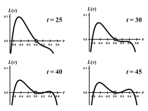That this can happen is explained by the fact that the adaptive landscape $L(x_t,u_t,v)$ changes with time; see Figure 2 in Section 4.1.

Figure 1. Two examples are shown for Equations (20(20) $\begin{array}{rl}x(t+1)& =[(b{s}_n-s_a)\exp (-w_0{u}^2\left(t\right))+s_a]\frac{x\left(t\right)}{1+c_{0}x\left(t\right)}\end{array}$(20) ) and (21(21) $\begin{array}{rl}u(t+1)& =(1-2w_0{\sigma }^2\frac{(b{s}_n-s_a)\exp (-w_0{u}^2\left(t\right))}{(b{s}_n-s_a)\exp (-w_0{u}^2\left(t\right))+s_a})u\left(t\right).\end{array}$(21) ) with parameter values $w_0=5,$ $w_1=5.5$, $c_0=1,$ $s_a=0.25,$ $s_n=0.5,$ and ${\sigma }^2=0.01$. In both cases $b>b_0=1/s_n=2$ and Theorem 4.1 implies the existence of a globally stable positive equilibrium with a semelparous trait component. (a) b = 5: four typical orbits in the x, u-phase plane are seen to approach the equilibrium $(x,u)=(1.5,0)$, and the adaptive landscape $L(v)$ has a global maximum at u = 0. (b) b = 40: four typical orbits x, u-phase plane are seen to approach a positive equilibrium $(x,u)=(19.0,0),$ and the adaptive landscape $L(v)$ has a local minimum at u = 0.

Figure 2. Shown are selected time snapshots of the adaptive landscape for the simulation in Figure 2(b) for the orbit with initial condition $(x(0),u(0))=(30,0.2)$. The trait component $u_t$ moves to the left towards the peak (not easily perceptible on the scale shown), but asymptotically arrives at a local minimum on the equilibrium landscape (shown in Figure 1(b)).

4. Two Darwinian models with reproductive-survival trade-offs

A central role in studies of life-history theory is played by reproductive strategies and central to those are trade-offs between reproductive effort and post-reproductive survival. The allocation of more resources towards higher reproductive effort often comes at the cost of fewer resources placed into processes affecting post-reproductive survival. An extreme case is semelparity, the life-history strategy in which individuals reproduce only once in their life time and die afterward. In an influential paper, Cole [6] argued that evolution should favour this strategy which, because iteroparity (possessing more than one reproductive episode per lifetime) is pervasive throughout nature, became known as Cole's paradox. Many critiques of Cole's argument and resolutions of the paradox (i.e. explanations for how iteroparity can arise by evolutionary or environmental processes) have been offered. These are based on a variety of mechanisms and circumstances such as fertility-survival trade-offs, nonlinear density effects, fluctuating environments and bet-hedging, spacial effects, and combinations of these [29,33]. Here we investigate the first two of these mechanisms by using model equations of the form (1(1) $r(x):=fb\beta (x)s_n\alpha (x)+(1-f)s_a\gamma (x)$(1) )–(5(5) $\begin{array}{rl}x(t+1)& ={r(x\left(t\right),u\left(t\right),v)|}_{v=u\left(t\right)}x\left(t\right)\end{array}$(5) )–(6(6) $\begin{array}{rl}u(t+1)& =u\left(t\right)+{\sigma }^2{\frac{\mathrm{\partial }\ln r(x\left(t\right),u\left(t\right),v)}{\mathrm{\partial }v}|}_{v=u\left(t\right)}.\end{array}$(6) ).

The goal is to determine what circumstances lead to equilibrium states with low post-reproductive survival and which lead to high post-reproductive survival. As we will see, there is no general answer to this question, even for the relatively simply low dimensional model (1(1) $r(x):=fb\beta (x)s_n\alpha (x)+(1-f)s_a\gamma (x)$(1) )–(5(5) $\begin{array}{rl}x(t+1)& ={r(x\left(t\right),u\left(t\right),v)|}_{v=u\left(t\right)}x\left(t\right)\end{array}$(5) )–(6(6) $\begin{array}{rl}u(t+1)& =u\left(t\right)+{\sigma }^2{\frac{\mathrm{\partial }\ln r(x\left(t\right),u\left(t\right),v)}{\mathrm{\partial }v}|}_{v=u\left(t\right)}.\end{array}$(6) ). Which strategy is selected by evolution is model dependent, specifically, is significantly dependent on the type of density factors used and on the manner in which they depend on the evolving trait.

We illustrate the diversity of possible outcomes by means of two examples selected to illustrate two different model predictions. Both models are based on an m = 1 dimensional population equation and a single n = 1 phenotypic trait. The first example is an evolutionary version of the discrete logistic (Beverton–Holt) equation with a type of density trait dependence called symmetric. The second example includes an Allee component with a hierarchical (or asymmetric) trait dependence. In both examples, we assume that fertility has a Gauss-type distribution with respect to the trait v $f\left(v\right)=\exp (-w_0{v}^2),w_0>0.$Thus, individuals with trait v = 0 attain maximal fertility b, but as a result have a post-reproductive survival rate of 0 (i.e. are semelparous).

We also assume that the effect that population density has on an individual's fertility and survival depends on both the individual's trait v and the population mean trait u. This assumed dependence on u reflects the fact that density effects involve intraspecific interactions. More specifically we assume (as is often done in Darwinian models [40]) that the density factors depend on the difference v−u, that is to say, the effects that intraspecific interactions have on an individual depends on how different its trait v is from the typical individual in the population. Finally, in these examples, we use the maximal fertility rate as a bifurcation parameter $\mu =b.$

4.1. A logistic model

In (1(1) $r(x):=fb\beta (x)s_n\alpha (x)+(1-f)s_a\gamma (x)$(1) )–(5(5) $\begin{array}{rl}x(t+1)& ={r(x\left(t\right),u\left(t\right),v)|}_{v=u\left(t\right)}x\left(t\right)\end{array}$(5) )–(6(6) $\begin{array}{rl}u(t+1)& =u\left(t\right)+{\sigma }^2{\frac{\mathrm{\partial }\ln r(x\left(t\right),u\left(t\right),v)}{\mathrm{\partial }v}|}_{v=u\left(t\right)}.\end{array}$(6) ), we take density factors $\beta (x)\equiv 1$ and $\alpha (x,v-u)=\gamma (x,v-u)=\frac{1}{1+c(v-u)x}.$This describes a situation in which the only density effects in play are negative effects on newborn and adult survival probabilities, both in the same way. An expression commonly used for the trait dependence of the competition coefficient is [40] $c(v-u)=c_0\exp (-w_1{(v-u)}^2),w_1>0.$This implies that the maximal value of the intraspecific competition coefficient, namely $c_0$, occurs when $v=u,$ i.e. when the individual's trait is equal to that of a typical individual it is likely to encounter, as represented by the population mean. Note that this modelling assumption implies $c(v-u)$ symmetric in the difference v−u.

Under these modelling assumptions, we have $r(b,x,u,v)=[b{s}_n\exp (-w_0{v}^2)+s_a(1-\exp (-w_0{v}^2)]\frac{1}{1+c(v-u)x}$and A1 and A2 are easily seen to hold on the domain $D=R_{+}^1\times {\mathrm{\Omega }}_x\times R^1\times R^1$ where ${\mathrm{\Omega }}_x$ is the half line $x>-1/c_0$. The Darwinian Equations (1(1) $r(x):=fb\beta (x)s_n\alpha (x)+(1-f)s_a\gamma (x)$(1) )–(5(5) $\begin{array}{rl}x(t+1)& ={r(x\left(t\right),u\left(t\right),v)|}_{v=u\left(t\right)}x\left(t\right)\end{array}$(5) )–(6(6) $\begin{array}{rl}u(t+1)& =u\left(t\right)+{\sigma }^2{\frac{\mathrm{\partial }\ln r(x\left(t\right),u\left(t\right),v)}{\mathrm{\partial }v}|}_{v=u\left(t\right)}.\end{array}$(6) ) become(20) $\begin{array}{rl}x(t+1)& =[(b{s}_n-s_a)\exp (-w_0{u}^2\left(t\right))+s_a]\frac{x\left(t\right)}{1+c_{0}x\left(t\right)}\end{array}$(20) (21) $\begin{array}{rl}u(t+1)& =(1-2w_0{\sigma }^2\frac{(b{s}_n-s_a)\exp (-w_0{u}^2\left(t\right))}{(b{s}_n-s_a)\exp (-w_0{u}^2\left(t\right))+s_a})u\left(t\right).\end{array}$(21) A3 holds for ${\hat{u}}_0=0$ and $(x,u)=(0,0)$ is an extinction equilibrium for all values of $b>0.$

It is not difficult to see, for all initial conditions $x_0\ge 0$, that $b{s}_n-s_a\le 0$ implies $x(t+1)<s_{a}x(t)$ and hence that $x(t)\to 0$ as $t\to \mathrm{\infty }.$ Therefore, we assume from now on that $b{s}_n>s_a.$A calculation shows $H(\mu ,{\hat{0}}_m,{\hat{u}}_0,{\hat{u}}_0)=(\mu s_n-s_a)f^{\mathrm{\prime }\mathrm{\prime }}\left(0\right)=-2w_0(b{s}_n-s_a)<0$and hence A4 holds. Finally, from $r(b,0,0,0)=b{s}_n$ we find that A5 holds with ${\mu }_0=b_0=1/s_n$ (since $d=s_n>0$).

Theorems 3.1 implies that the extinction equilibrium $(0,0)$ loses stability as $\mu =b$ increases through $b_0:=1/s_n$. Theorem 3.3 in turn implies, provided ${\sigma }^2$ is sufficiently small, the forward bifurcation of stable positive equilibria for $b>b_0$.

We can obtain more results for (20(20) $\begin{array}{rl}x(t+1)& =[(b{s}_n-s_a)\exp (-w_0{u}^2\left(t\right))+s_a]\frac{x\left(t\right)}{1+c_{0}x\left(t\right)}\end{array}$(20) ) and (21(21) $\begin{array}{rl}u(t+1)& =(1-2w_0{\sigma }^2\frac{(b{s}_n-s_a)\exp (-w_0{u}^2\left(t\right))}{(b{s}_n-s_a)\exp (-w_0{u}^2\left(t\right))+s_a})u\left(t\right).\end{array}$(21) ) by noting the scalar difference Equation (21(21) $\begin{array}{rl}u(t+1)& =(1-2w_0{\sigma }^2\frac{(b{s}_n-s_a)\exp (-w_0{u}^2\left(t\right))}{(b{s}_n-s_a)\exp (-w_0{u}^2\left(t\right))+s_a})u\left(t\right).\end{array}$(21) ) is uncoupled from Equation (20(20) $\begin{array}{rl}x(t+1)& =[(b{s}_n-s_a)\exp (-w_0{u}^2\left(t\right))+s_a]\frac{x\left(t\right)}{1+c_{0}x\left(t\right)}\end{array}$(20) ). Straightforward manipulations of inequalities show that $-1<1-2w_0{\sigma }^2\frac{(b{s}_n-s_a)f\left(u\right)}{(b{s}_n-s_a)f\left(u\right)+s_a}<1$for all $b>s_a/s_n$ provided ${\sigma }^2<1/w_0.$ It follows, under this condition on ${\sigma }^2$, that $|u(t+1)|<|u(t)|$ and consequently all solutions (21(21) $\begin{array}{rl}u(t+1)& =(1-2w_0{\sigma }^2\frac{(b{s}_n-s_a)\exp (-w_0{u}^2\left(t\right))}{(b{s}_n-s_a)\exp (-w_0{u}^2\left(t\right))+s_a})u\left(t\right).\end{array}$(21) ) tend to 0 as $t\to +\mathrm{\infty }.$ Thus, for any initial condition $u(0)$, the Equation (20(20) $\begin{array}{rl}x(t+1)& =[(b{s}_n-s_a)\exp (-w_0{u}^2\left(t\right))+s_a]\frac{x\left(t\right)}{1+c_{0}x\left(t\right)}\end{array}$(20) ) is asymptotically autonomous with limiting equation $x(t+1)=b{s}_n\frac{1}{1+c_{0}x\left(t\right)}x\left(t\right).$For this (discrete logistic) equation It is well known that x = 0 is globally asymptotically stable if $b{s}_n<1$. If $b{s}_n>1$ the positive equilibrium $x=(b{s}_n-1)/c_0$ is globally asymptotically stable for $x(0)>0$. Theorems dealing with asymptotically autonomous difference equations (for example see Theorem 4 in [9]) imply the following results.

Theorem 4.1

Consider the Darwinian model Equations (20(20) $\begin{array}{rl}x(t+1)& =[(b{s}_n-s_a)\exp (-w_0{u}^2\left(t\right))+s_a]\frac{x\left(t\right)}{1+c_{0}x\left(t\right)}\end{array}$(20) ) and (21(21) $\begin{array}{rl}u(t+1)& =(1-2w_0{\sigma }^2\frac{(b{s}_n-s_a)\exp (-w_0{u}^2\left(t\right))}{(b{s}_n-s_a)\exp (-w_0{u}^2\left(t\right))+s_a})u\left(t\right).\end{array}$(21) ).

1. If $b\le b_0:=1/s_n$, then $x(t)\to 0$ as $t\to +\mathrm{\infty }$ for all initial conditions $u(0)$ and $x(0)\ge 0.$

2. Assume ${\sigma }^2<1/w_0$. If $b>b_0$ then the extinction equilibrium $(x,u)=(0,0)$ is unstable and the positive equilibrium $(x,u)=((b{s}_n-1)/c_0,0)$ is globally asymptotically stable for all initial conditions $u(0)$ and $x(0)>0$.

A take away message from this theorem is that, under the modelling assumption made in this example, the only possible positive equilibria have mean trait component $u=0,$ i.e. are semelparous equilibria, which is in accord with Cole's assertion [6]. However, is u = 0 and ESS trait? That is to say, does the adaptive landscape $\begin{array}{rl}L(v)& :=\ln r(b,\frac{b{s}_n-1}{c_0},v,0)\\ & =\ln [(b{s}_n-s_a)\exp (-w_0{v}^2)+s_a]-\ln (1+(b{s}_n-1)\exp (-w_1{v}^2))\end{array}$attain a global maximum at v = 0? Near the bifurcation point $b{s}_n=1$ the landscape is approximately $L(v)\approx \ln [(1-s_a)\exp (-w_0{v}^2)+s_a]$, which has a global maximum at v = 0 and the positive equilibrium is an ESS. For larger $b{s}_n$, however, the answer depends on the ratio $w_0/w_1$. Calculations show $L\left(0\right)=0,\frac{\mathrm{d}L\left(0\right)}{\mathrm{d}v}=0,\frac{{\mathrm{d}}^{2}L\left(0\right)}{\mathrm{d}{v}^2}=2w_0\frac{b{s}_n-1}{b{s}_n}(\frac{w_1}{w_0}-\frac{b{s}_n-s_a}{b{s}_n-1}).$From these, we see that (22) $\frac{w_1}{w_0}>\frac{b{s}_n-s_a}{b{s}_n-1}$(22) implies the landscape has a local minimum at $v=0$and in this case the equilibrium trait is not an ESS. Near the bifurcation point $b{s}_n⪆1$ the semelparous equilibrium is an ESS, but if $b{s}_n$ is large enough that (22(22) $\frac{w_1}{w_0}>\frac{b{s}_n-s_a}{b{s}_n-1}$(22) ) holds then it is not an ESS. See Figure 1 for numerical simulations that illustrate this loss of ESS status. In Figure 1, it is perhaps counter-intuitive that the trait component of a positive equilibrium is located at a minimum on the adaptive landscape, since the trait equation in a Darwinian model implies that $u(t)$ moves uphill on the landscape. The explanation lies in the fact that the landscape changes over time, which can (and does in Figure 1(b)) allow for uphill movement that ends in a valley. See Figure 2.

4.2. A model with an allee component

Our second example is a Darwinian model (1(1) $r(x):=fb\beta (x)s_n\alpha (x)+(1-f)s_a\gamma (x)$(1) )–(5(5) $\begin{array}{rl}x(t+1)& ={r(x\left(t\right),u\left(t\right),v)|}_{v=u\left(t\right)}x\left(t\right)\end{array}$(5) )–(6(6) $\begin{array}{rl}u(t+1)& =u\left(t\right)+{\sigma }^2{\frac{\mathrm{\partial }\ln r(x\left(t\right),u\left(t\right),v)}{\mathrm{\partial }v}|}_{v=u\left(t\right)}.\end{array}$(6) ) that is again designed to investigate trait dependent fertility-survival trade-offs and density effects, but under different assumptions from those made in Section 4.1. This model will, unlike the model Section 4.1, allow for ESS traits that yield high post-reproductive survival (iteroparity).

We consider a model the incorporates density effects in adult fertility $\beta (x)$ and newborn survival $\alpha (x)$ (and ignores density effects on adult survival $\gamma (x)\equiv 1$). Specifically, we assume population density affects adult fertility in a negative way, again given by the factor (2(2) $\frac{1}{1+cx}\mathrm{with}c>0.$(2) ) $\beta \left(x\right)=\frac{1}{1+cx}$but affects newborn survival in a positive way by using a factor $\alpha (x)$ of the form (3(3) $\frac{1+\rho a{x}^q}{1+a{x}^q}\mathrm{with}q\ge 1,a\ge 0\mathrm{and}\rho >1$(3) ), namely $\alpha \left(x\right)=\frac{1+\rho a{x}^q}{1+a{x}^q},a\ge 0\mathrm{and}1<\rho <1/s_n$where we take $q\ge 1$ to be an integer. This factor is the fractional increase of the inherent newborn survival rate $s_n$ as a function of increasing population density. Such a so-called component Allee effect can be the result of numerous mechanisms [7], an example of which is increased protection of newborns from predators by adults. Under this assumption with a > 0, newborn survival probability increases from $s_n$ to $\rho s_n$ as population density x increases without bound. We will refer to a as the Allee coefficient since it measures how quickly newborn survival increases with x, as can be seen by the fact that newborn survival reaches the midpoint $s_n(1+\rho )/2$ at $x=1/a^{1/q}$; this midpoint is reached more quickly for large values of a > 0.

In the Darwinian model (5(5) $\begin{array}{rl}x(t+1)& ={r(x\left(t\right),u\left(t\right),v)|}_{v=u\left(t\right)}x\left(t\right)\end{array}$(5) )–(6(6) $\begin{array}{rl}u(t+1)& =u\left(t\right)+{\sigma }^2{\frac{\mathrm{\partial }\ln r(x\left(t\right),u\left(t\right),v)}{\mathrm{\partial }v}|}_{v=u\left(t\right)}.\end{array}$(6) ) equations, we assume in this example that both the competition and Allee coefficients are trait dependent. In contrast to the example in Section 4.1, we assume the competition coefficient has an asymmetric trait dependence [25]. Specifically, we take $c(v-u)=c_0\exp (-w_1(v-u)),w_1>0.$This assumption can be viewed as describing a hierarchical dependence of intra-specific competition on the trait in that individuals with larger traits are subject to less intraspecific competition. Since $c(0)=c_0$, the coefficient $c_0$ measures the effect of competition experienced by the typical individual with trait v = u.

Finally, we assume the Allee coefficient is an increasing function of the population mean trait u so that newborns of all traits are (equally) benefitted by a population with larger mean trait. Specifically, in this example, we take $a=a_0{u}^2$. In summary, these assumption imply roughly that as an individual's trait v > 0 increases it obtains higher post-reproductive survival probably in trade-off with decreased inherent fertility, which is to some degree compensated for by both a lower competition coefficient and a higher Allee coefficient. These would suggest the possibility of positive equilibrium states that have trait component different from 0 (in contrast to the example in Section 4.1) and hence the possibility of significant post-reproductive survival.

With these modelling choices, we have (23) $r(b,x,u,v)=b{e}^{-w_0{v}^2}\frac{1}{1+c_0{e}^{-w_1(v-u)}x}{s}_n\frac{1+\rho a_0{u}^2{x}^q}{1+a_0{u}^2{x}^q}+s_a(1-e^{-w_0{v}^2})$(23) in the Darwinian Equations (5(5) $\begin{array}{rl}x(t+1)& ={r(x\left(t\right),u\left(t\right),v)|}_{v=u\left(t\right)}x\left(t\right)\end{array}$(5) ) and (6(6) $\begin{array}{rl}u(t+1)& =u\left(t\right)+{\sigma }^2{\frac{\mathrm{\partial }\ln r(x\left(t\right),u\left(t\right),v)}{\mathrm{\partial }v}|}_{v=u\left(t\right)}.\end{array}$(6) ). We again choose $\mu =b$ as the bifurcation parameter to be used in Theorems 3.2 and 3.3, for which we need to verify assumptions A1–A5.

First, we note that if $b{s}_n\le s_a$ then $r(b,x,u,v)x\le s_{a}x$ for all $x\ge 0$ and for all $v,u.$ Since $s_a<1$ it follows in this case that the population goes asymptotically extinct regardless of the trait dynamics, i.e. $x(t)\to 0$ as $t\to +\mathrm{\infty }$ for all initial conditions $x(0)$ and $u(0)$. Therefore, we assume from now on that $b{s}_n>s_a.$Under this added assumption, we turn our attention to assumptions A1–A5.

The $1\times 1$ projection and variance/covariance matrices are $P(b,x,u,v)=[r(b,x,u,v)]$ and $M=[{\sigma }^2]$. Equation (8(8) $0={\frac{\mathrm{\partial }r(0,u_0,v)}{\mathrm{\partial }v}|}_{v=u_0}$(8) ) for critical traits $u_0$ that define extinction equilibria $(x_e,u_e)=(0,u_0)$ is $0=2w_0(s_a-b{s}_n)u_0{e}^{-w_0{u}_0^2}.$With the parameter interval ${\mathrm{\Omega }}_{\mu }$ taken to be the half line $\mu =b>s_a/s_n$ and the trait interval ${\mathrm{\Omega }}_n={\mathrm{\Omega }}_1$ to be $R^1,$ it is straightforward to verify that assumptions A1, A2, and A3 hold if ${\sigma }^2>0$ (evolution occurs) and that $(x_e,u_e)=(0,0)$ is an extinction equilibrium for all $b\in {\mathrm{\Omega }}_{\mu }$. The $1\times 1$ Hessian $H(b,0,0,0)=[-2w_0(b-s_a)/b{s}_n]$is nonsingular for $b\in {\mathrm{\Omega }}_{\mu }$ which implies assumption A4 holds. Finally, simple calculations show $r(b_0,0,0,0)=1$ if and only if $b_0=1/s_n$ and $d=s_n$ and hence that assumption A5 holds. Note that $b_0>1>s_a.$

The $1\times 1$ projection matrix $P(b_0,0,0,0)=[1]$ is primitive and the only eigenvalue $-2w_0(b-s_a)/b{s}_n$ of the $1\times 1$ Hessian $H(b_0,0,0,0)$ is negative. Moreover, $d=s_n>0$ and $\kappa :=-{\mathrm{\partial }}_{x}r(b_0,{\hat{0}}_m,0,0)=b_0{s}_n{c}_0>0.$With assumptions A1–A5 verified, we obtain the following theorem from Theorems 3.1(a), 3.2, and 3.3(a).

Theorem 4.2

For the Darwinian Equations (5(5) $\begin{array}{rl}x(t+1)& ={r(x\left(t\right),u\left(t\right),v)|}_{v=u\left(t\right)}x\left(t\right)\end{array}$(5) ) and (6(6) $\begin{array}{rl}u(t+1)& =u\left(t\right)+{\sigma }^2{\frac{\mathrm{\partial }\ln r(x\left(t\right),u\left(t\right),v)}{\mathrm{\partial }v}|}_{v=u\left(t\right)}.\end{array}$(6) ) with (23(23) $r(b,x,u,v)=b{e}^{-w_0{v}^2}\frac{1}{1+c_0{e}^{-w_1(v-u)}x}{s}_n\frac{1+\rho a_0{u}^2{x}^q}{1+a_0{u}^2{x}^q}+s_a(1-e^{-w_0{v}^2})$(23) ), under the assumption that ${\sigma }^2$ is sufficiently small, the extinction equilibrium $(x_e,u_e)=(0,0)$ destabilizes as b increases through $b_0=1/s_n$ and a forward bifurcation of (locally asymptotically) stable positive equilibria occurs.

Remark 4.1

We can obtain an upper bound for how small ${\sigma }^2$ must be in Theorem 4.2 from a consideration of the proof of Theorem 3.1 in the Appendix. The assumption of small ${\sigma }^2$ is only needed so as to insure that the eigenvalue values of lower right block $I_n+MH(\mu ,{\hat{0}}_m,{\hat{u}}_0,{\hat{u}}_0)$ in the block diagonal Jacobian $\mathfrak{J}(\mu ,{\hat{0}}_m,{\hat{u}}_0,{\hat{u}}_0)$ are all less than 1 in absolute value. Then it is the eigenvalues of the upper left block $P(\mu ,{\hat{0}}_m,{\hat{u}}_0,{\hat{u}}_0)$ that determine stability (by linearization). For the Equations (5(5) $\begin{array}{rl}x(t+1)& ={r(x\left(t\right),u\left(t\right),v)|}_{v=u\left(t\right)}x\left(t\right)\end{array}$(5) ) and (6(6) $\begin{array}{rl}u(t+1)& =u\left(t\right)+{\sigma }^2{\frac{\mathrm{\partial }\ln r(x\left(t\right),u\left(t\right),v)}{\mathrm{\partial }v}|}_{v=u\left(t\right)}.\end{array}$(6) ) both blocks are $1\times 1$, i.e. are simply scalars. In particular, the eigenvalue $1+{\sigma }^2{\mathrm{\partial }}_v^2\ln r(b_0,0,0,0)=1-{\sigma }^{2}2w_0\frac{1-s_a{s}_n}{s_n}$of $I_n+MH(\mu ,{\hat{0}}_m,{\hat{u}}_0,{\hat{u}}_0)=[1+{\sigma }^2{\mathrm{\partial }}_v^2\ln r(b_0,0,0,0)]$is clearly less than 1. It is greater than $-1$ if and only if ${\sigma }^2<\frac{1}{w_0}\frac{s_n}{1-s_a{s}_n},$which is how small ${\sigma }^2$ must be in Theorem 4.2.

Theorems 3.2 and 3.3(a) are local bifurcation results and hence Theorem 4.2 accounts for the bifurcating equilibria and their stability only in a neighbourhood of the bifurcation point, i.e. for $b\approx b_0$ and $(x_e,u_e)$ near $(0,0)$. In this neighbourhood, the bifurcating positive equilibria have trait components $u_e$ near 0 and therefore yield populations that, at equilibrium, have low post-reproductive survival (semelparity). However, outside a neighbourhood of the bifurcation point, this Darwinian model can have equilibria with a high post-reproductive survival rates. While we have no mathematical proof of this, we illustrate this possibility by means of the selected numerical simulations shown in Figures 3 and 4.

Figure 3. Two phase plane orbits are shown for the Darwinian model (5(5) $\begin{array}{rl}x(t+1)& ={r(x\left(t\right),u\left(t\right),v)|}_{v=u\left(t\right)}x\left(t\right)\end{array}$(5) )–(6(6) $\begin{array}{rl}u(t+1)& =u\left(t\right)+{\sigma }^2{\frac{\mathrm{\partial }\ln r(x\left(t\right),u\left(t\right),v)}{\mathrm{\partial }v}|}_{v=u\left(t\right)}.\end{array}$(6) )–(23(23) $r(b,x,u,v)=b{e}^{-w_0{v}^2}\frac{1}{1+c_0{e}^{-w_1(v-u)}x}{s}_n\frac{1+\rho a_0{u}^2{x}^q}{1+a_0{u}^2{x}^q}+s_a(1-e^{-w_0{v}^2})$(23) ) with parameters values $b=3.4,$ $w_0=1,$ $c_0=0.2,$ $w_1=1,$ $\rho =3,$ $a_0=0.2,$ $s_n=0.3,$ $s_a=0.9,$ $q=2,$ ${\sigma }^2=\mathrm{0.4.}$ Note that $b>b_0=1/s_n=10/3$ and hence the extinction equilibrium $(0,0)$ is unstable. The orbit with initial condition $(x(0),u(0))=(5,0)$ approaches the positive equilibrium $(x_1,u_1)=(0.096,0.093)$ (open square), which is the bifurcating equilibrium from the extinction equilibrium $(0,0)$ predicted by Theorem 4.2. The orbit with initial condition $(x(0),u(0))=(6,0)$ approaches a different equilibrium, namely. $(x_2,u_2)=(6.789,1.086)$ (open square). Both equilibrium trait values lie on global maxima of their respective adaptive landscapes $L(v)$ (open squares) and hence are ESS traits.

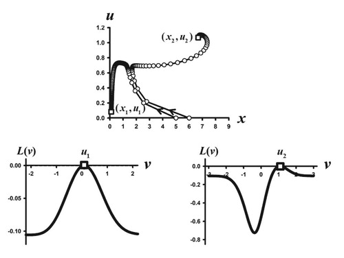
Figure 4. Two phase plane orbits are shown for the Darwinian model (5(5) $\begin{array}{rl}x(t+1)& ={r(x\left(t\right),u\left(t\right),v)|}_{v=u\left(t\right)}x\left(t\right)\end{array}$(5) )–(6(6) $\begin{array}{rl}u(t+1)& =u\left(t\right)+{\sigma }^2{\frac{\mathrm{\partial }\ln r(x\left(t\right),u\left(t\right),v)}{\mathrm{\partial }v}|}_{v=u\left(t\right)}.\end{array}$(6) )–(23(23) $r(b,x,u,v)=b{e}^{-w_0{v}^2}\frac{1}{1+c_0{e}^{-w_1(v-u)}x}{s}_n\frac{1+\rho a_0{u}^2{x}^q}{1+a_0{u}^2{x}^q}+s_a(1-e^{-w_0{v}^2})$(23) ) with the same parameters values as in Figure 3 except that b has been changed to b = 3.2. Since $b<b_0=1/s_n=10/3$ the extinction equilibrium $(x_1,u_1)=(0,0)$ is stable, as is illustrated by the orbit with initial condition $(x(0),u(0))=(8,0)$. However, the orbit with initial condition $(x(0),u(0))=(9,0)$ approaches a positive equilibrium $(x_2,u_2)=(6.036,1.065)$, whose trait component is an ESS as the accompanying graph of the adaptive landscape $L(v)$ shows.

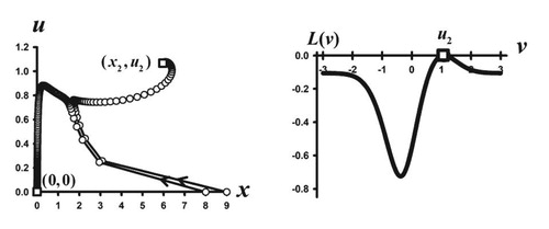
Figure 3 illustrates the bifurcation described in Theorem 4.2, for selected parameter values, when b is greater that $1/s_n$ (hence the extinction equilibrium is unstable) but is close to $1/s_n$. In the x, u-phase plane, the orbit with initial condition $(x(0),u(0))=(5,0)$ is shown approaching the equilibrium $(x_1,u_1)=(0.096,0.093)$, which is near the extinction equilibrium $(0,0)$ as predicted by Theorem 4.2. However, Figure 3 also illustrates another phenomenon, namely that in this sample case there exists a second positive equilibrium $(x_2,u_2)=(6.789,1.086),$ which is approached by the orbit with initial condition $(x(0),u(0))=(6,0)$. This example case in Figure 3 suggests a multi-attractor scenario in which the asymptotic, equilibrium states of orbits are initial condition dependent. This is not precluded by Theorem 4.2 since that theorem only concerns a local bifurcation of positive equilibrium near the extinction equilibrium.

Also shown in Figure 3 are the adaptive landscapes at each of these two equilibria and how the trait component of each equilibrium lies at a global maximum of its respective adaptive landscape. Thus, both equilibria have ESS trait components. Note that the post-reproductive survival probability $s_a(1-f(u_1))=0.008$ at the equilibrium $(x_1,u_1)$ is quite low, while it is significantly higher at the equilibrium $(x_2,u_2)$, namely $s_a(1-f(u_2))=0.623$. Therefore, in this sample case, whether evolution selects for a low or high post-reproductive survival rate is initial condition dependent.

Figure 4 shows another interesting phenomenon that can occur in the model (5(5) $\begin{array}{rl}x(t+1)& ={r(x\left(t\right),u\left(t\right),v)|}_{v=u\left(t\right)}x\left(t\right)\end{array}$(5) )–(6(6) $\begin{array}{rl}u(t+1)& =u\left(t\right)+{\sigma }^2{\frac{\mathrm{\partial }\ln r(x\left(t\right),u\left(t\right),v)}{\mathrm{\partial }v}|}_{v=u\left(t\right)}.\end{array}$(6) ) with (23(23) $r(b,x,u,v)=b{e}^{-w_0{v}^2}\frac{1}{1+c_0{e}^{-w_1(v-u)}x}{s}_n\frac{1+\rho a_0{u}^2{x}^q}{1+a_0{u}^2{x}^q}+s_a(1-e^{-w_0{v}^2})$(23) ). It shows two-phase plane orbits in a case when $b<1/s_n$ and the extinction equilibrium is stable. One orbit does approach the extinction equilibrium, but the other approaches a positive equilibrium. This suggests that a strong Allee effect [7] occurs in this example, which means survival is initial condition dependent. The trait component of the positive equilibrium is an ESS (see Figure 4) and yields a high post-reproductive survival of $s_a(1-f(u_2))=0.611$. Strong Allee effects arise in population models most commonly due to a backward bifurcation [11]; however, in this case, the bifurcation is forward.

A rigorous mathematical treatment of positive equilibria outside a neighbourhood of the bifurcation point remains an open problem. In the next Section 5, we offer a plausible, but unproved, explanation of the multi-attractor cases suggested by Figures 3 and 4.

5. Concluding remarks

In Section 4, we applied the general bifurcation theorems in Section 3 for Darwinian matrix models to a low dimensional model (5(5) $\begin{array}{rl}x(t+1)& ={r(x\left(t\right),u\left(t\right),v)|}_{v=u\left(t\right)}x\left(t\right)\end{array}$(5) ) and (6(6) $\begin{array}{rl}u(t+1)& =u\left(t\right)+{\sigma }^2{\frac{\mathrm{\partial }\ln r(x\left(t\right),u\left(t\right),v)}{\mathrm{\partial }v}|}_{v=u\left(t\right)}.\end{array}$(6) ) designed to study the evolution post-reproductive survival and to address Cole's paradox that evolution should favour semelparity. The models focus on two trait dependent mechanisms: inherent fertility-versus-survival trade-offs and density effects. In both models, fertility is assumed to have a Gaussian distribution with respect to the phenotypic trait v.

The model studied in Section 4.1 assumes logistic density effects on newborns and adults and a trait dependent intra-specific competition coefficient that is a symmetric function of the different v−u. This model supports Cole's assertion in that it predicts that the only survival equilibria have an ESS semelparous trait. In contrast, the model studied in Section 4.2 includes an Allee component in the density effect on juvenile survival and a trait dependent intra-specific competition coefficient that is a asymmetric (monotone) function of the different v−u. The fundamental bifurcation that occurs upon destabilization of the extinction equilibrium creates positive equilibria with low post-reproductive survival (Theorem 4.2). These equilibria again support Cole's contention that evolution favours semelparity. However, simulations of the model show that it is possible for the trait component of positive equilibria lying outside a neighbourhood of the bifurcation point to correspond to a high post-reproductive survival rate, which runs counter to Cole's contention (Figures 3 and 4). These simulations also suggest that these iteroparous equilibria can occur simultaneously with either semelparous equilibria or with the extinction equilibrium, in multiple attractor scenarios. While it remains an open mathematical question to establish these phenomena rigorously, a hint towards a possible mathematical explanation can be found in the bifurcation analysis of the non-evolutionary version of the model.

When the mean trait u is held fixed and not allowed to evolve (${\sigma }^2=0$), the two Equations (5(5) $\begin{array}{rl}x(t+1)& ={r(x\left(t\right),u\left(t\right),v)|}_{v=u\left(t\right)}x\left(t\right)\end{array}$(5) ) and (6(6) $\begin{array}{rl}u(t+1)& =u\left(t\right)+{\sigma }^2{\frac{\mathrm{\partial }\ln r(x\left(t\right),u\left(t\right),v)}{\mathrm{\partial }v}|}_{v=u\left(t\right)}.\end{array}$(6) ) reduce to just the scalar difference Equation (5(5) $\begin{array}{rl}x(t+1)& ={r(x\left(t\right),u\left(t\right),v)|}_{v=u\left(t\right)}x\left(t\right)\end{array}$(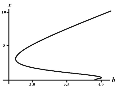5) ) whose (positive) equilibrium equation is (24) $b{e}^{-w_0{u}^2}\frac{1}{1+c_{0}x}{s}_n\frac{1+\rho a_0{u}^2{x}^2}{1+a_0{u}^2{x}^2}+s_a(1-e^{-w_0{u}^2})=1.$(24) For any fixed mean trait value u, a plot of x as a function b as defined by this equation, yields a equilibrium bifurcation diagram. An example is shown in Figure 5, using the same parameter values as in Figures 3 and 4, but with u fixed at u = 1 (which is near the equilibrium trait component for the positive equilibrium obtained from the Darwinian model used in Figures 3 and 4). The bifurcation diagram in Figure 5 shows the destabilization of the extinction equilibrium x = 0 as b increases through $b_0=3+e/3=3.91$ and multiple positive equilibria on an interval of b values less than $b_0$ where x = 0 is stable (as in Figure 3) and an interval of b values greater than $b_0$ on which there exists a multiple positive equilibria where x = 0 is unstable (as in Figure 4). It is known from general theorems that the positive equilibria on the decreasing segment in the bifurcation diagram are unstable, but that those on increasing segments, at least near the two tangent bifurcations, are (locally asymptotically) stable [12,14]. The hysteresis loop in this bifurcation diagram is due to the interplay of the negative and positive density effects described in the fertility and Allee factors β and α, respectively. While this is not the bifurcation diagram for the Darwinian model (5(5) $\begin{array}{rl}x(t+1)& ={r(x\left(t\right),u\left(t\right),v)|}_{v=u\left(t\right)}x\left(t\right)\end{array}$(5) )–(6(6) $\begin{array}{rl}u(t+1)& =u\left(t\right)+{\sigma }^2{\frac{\mathrm{\partial }\ln r(x\left(t\right),u\left(t\right),v)}{\mathrm{\partial }v}|}_{v=u\left(t\right)}.\end{array}$(6) )–(23(23) $r(b,x,u,v)=b{e}^{-w_0{v}^2}\frac{1}{1+c_0{e}^{-w_1(v-u)}x}{s}_n\frac{1+\rho a_0{u}^2{x}^q}{1+a_0{u}^2{x}^q}+s_a(1-e^{-w_0{v}^2})$(23) ) in which u dynamically evolves, it does suggest that perhaps these same alternates do occur in the Darwinian model, as is suggested by Figures 3 and 4, and is due to the presence of a hysteresis in the bifurcation diagram.

Figure 5. Shown is a plot of the Equation (24(24) $b{e}^{-w_0{u}^2}\frac{1}{1+c_{0}x}{s}_n\frac{1+\rho a_0{u}^2{x}^2}{1+a_0{u}^2{x}^2}+s_a(1-e^{-w_0{u}^2})=1.$(24) ) in the $(b,x)$-plane with parameter values used in Figures 3 and 4 and $u=1.$

The results in Section 4, and those in other studies of other low dimensional Darwinian models [13,15,20], show that the answer to the question of whether evolution favours semelparity or iteroparity is much more complicated than Cole's simple assertion that it favours semelparity. In these models, whether evolution selects in favour of low or high post-reproductive survival depends crucially on the details of how the evolving trait affects the birth versus survival trade-off and on the specifics of the density effects, with some circumstances favouring one reproductive strategy and others favouring the other strategy. Moreover, this selection can be initial condition dependent. Other complications are introduced by a nonlinear trait dependent inherent fertility versus survival trade-off [20] and multiple peaks in the fertility distribution $f(v)$ [13,20], neither of which we considered here, although there is evidence for them in nature [26,32].

Acknowledgments

The author thanks an anonymous reviewer for a very careful reading of the paper and for numerous suggestions that clarified several issues.

Disclosure statement

No potential conflict of interest was reported by the author.

Additional information

Funding

Author supported by National Science Foundation grant DMS-1407564.

Appendix

Proof of Theorem 3.2.

Equation (14(14) $\begin{array}{rl}{\hat{0}}_n& ={\mathrm{\nabla }}_{\hat{v}}r(\mu ,\hat{x},\hat{u},\hat{u}).\end{array}$(14) ) is satisfied by $(\hat{x},\hat{u})=({\hat{0}}_m,{\hat{u}}_0)$ when $\mu ={\mu }_0.$ To apply the implicit function theorem to (14(14) $\begin{array}{rl}{\hat{0}}_n& ={\mathrm{\nabla }}_{\hat{v}}r(\mu ,\hat{x},\hat{u},\hat{u}).\end{array}$(14) ) at this point, we need the nonsingularity of the Jacobian of ${\mathrm{\nabla }}_{\hat{v}}r(\mu ,\hat{x},\hat{u},\hat{u})$ with respect to $\hat{u}$ when evaluated at $({\hat{x}}_e,{\hat{u}}_e)=({\hat{0}}_m,{\hat{u}}_0)$ and $\mu ={\mu }_0$. The partial derivative of ${\mathrm{\partial }}_{v_j}\ln r(\mu ,\hat{x},\hat{u},\hat{u})$ with respect to $u_i$ is ${\mathrm{\partial }}_{u_i{v}_j}\ln r(\mu ,\hat{x},\hat{u},\hat{u})+{\mathrm{\partial }}_{v_i{v}_j}\ln r(\mu ,\hat{x},\hat{u},\hat{u})$. When evaluated at $({\hat{x}}_e,{\hat{u}}_e)=({\hat{0}}_m,{\hat{u}}_0)$ the first term vanishes by assumption A1. This implies that the Jacobian of ${\mathrm{\nabla }}_{\hat{v}}r(\mu ,\hat{x},\hat{u},\hat{u})$ with respect to $\hat{u}$ is nonsingular, when evaluated at $\mu ={\mu }_0$ and $(\hat{x},\hat{u})=({\hat{0}}_m,{\hat{u}}_0)$, equals the Hessian $H(\mu ,{\hat{0}}_m,{\hat{u}}_e,{\hat{u}}_e)$ and hence, by A4, is nonsingular. The implicit function theorem then implies that there exists a solution $\hat{u}=\hat{\upsilon }(\mu ,\hat{x})$ of Equation (14(14) $\begin{array}{rl}{\hat{0}}_n& ={\mathrm{\nabla }}_{\hat{v}}r(\mu ,\hat{x},\hat{u},\hat{u}).\end{array}$(14) ), which is twice continuously differentiable in a neighbourhood of $\mu ={\mu }_0$ and $\hat{x}={\hat{0}}_m$, that satisfies $\hat{\upsilon }({\mu }_0,{\hat{0}}_m)=u_0$. Substituting this solution into Equation (13(13) $\begin{array}{rl}\hat{x}& =P(\mu ,\hat{x},\hat{u},\hat{u})\hat{x}\end{array}$(13) ), we are then tasked to solve the equation $\hat{x}=P(\mu ,\hat{x},\hat{\upsilon }(\mu ,\hat{x}),\hat{\upsilon }(\mu ,\hat{x}))\hat{x}$for $\hat{x}\in R_{+}^m$ as a function of μ. To do this we apply Theorem 3.1 in [16] to the equation (A1) $\hat{x}=\overline{P}(\mu ,\hat{x})\hat{x}$(A1) where $\overline{P}(\mu ,\hat{x})=[{\overline{p}}_{ij}(\mu ,\hat{x})]$ is defined by ${\overline{p}}_{ij}(\mu ,\hat{x}):=p_{ij}(\mu ,\hat{x},\hat{\upsilon }(\mu ,\hat{x}),\hat{\upsilon }(\mu ,\hat{x}))$. To apply this theorem it is required that:

1. $\overline{P}(\mu ,\hat{x})$ is nonnegative and irreducible;

2. the entries in $\overline{P}(\mu ,\hat{x})$ are twice continuously differentiable in a neighbourhood of $(\mu ,\hat{x})=({\mu }_0,{\hat{0}}_m);$

3. $\overline{P}({\mu }_0,{\hat{0}}_m)=P({\mu }_0,{\hat{0}}_m,{\hat{u}}_0,{\hat{u}}_0)$ has dominant eigenvalue value $r({\mu }_0,{\hat{0}}_m,{\hat{u}}_0,{\hat{u}}_0)=1;$

4. ${\tilde{w}}_L^T{\mathrm{\partial }}_{\mu }\overline{P}({\mu }_0,{\hat{0}}_m){\tilde{w}}_R\ne 0.$

(a) follows from A1, (b) follows from A1 together with the smoothness of $\hat{\upsilon }(\mu ,\hat{x})$ obtained from the implicit function theorem, and (c) follows from A5. Inequality (d) also follow from A5 because ${\tilde{w}}_L^T{\mathrm{\partial }}_{\mu }\overline{P}({\mu }_0,{\hat{0}}_m){\tilde{w}}_R=d$. To see this one only needs to note that ${\mathrm{\partial }}_{\mu }\hat{\upsilon }({\mu }_0,{\hat{0}}_m)={\hat{0}}_n$, a fact that follows from an implicit differentiation of ${\hat{0}}_n={\mathrm{\nabla }}_{\hat{v}}r(\mu ,\hat{x},\hat{\upsilon }(\mu ,\hat{x}),\hat{\upsilon }(\mu ,\hat{x}))$with respect to μ evaluated at $(\mu ,\hat{x})=({\mu }_0,{\hat{0}}_m)$ which yields $\begin{array}{rl}{\hat{0}}_n& ={\mathrm{\partial }}_{\mu }{\mathrm{\nabla }}_{\hat{v}}r({\mu }_0,{\hat{0}}_m,{\hat{u}}_0,{\hat{u}}_0)+{\mathrm{\nabla }}_{\hat{u}}{\mathrm{\nabla }}_{\hat{v}}r({\mu }_0,{\hat{0}}_m,{\hat{u}}_0,{\hat{u}}_0){\mathrm{\partial }}_{\mu }\hat{\upsilon }({\mu }_0,{\hat{0}}_m)\\ & +{\mathrm{\nabla }}_{\hat{v}}{\mathrm{\nabla }}_{\hat{v}}r({\mu }_0,{\hat{0}}_m,{\hat{u}}_0,{\hat{u}}_0){\mathrm{\partial }}_{\mu }\hat{\upsilon }({\mu }_0,{\hat{0}}_m).\end{array}$The first term on the left side of this equation vanishes by assumption A3 and the middle term vanishes by A1 (see Remark 3.1). The equation then reduces to ${\hat{0}}_n=H({\mu }_0,{\hat{0}}_m,{\hat{u}}_0,{\hat{u}}_0){\mathrm{\partial }}_{\mu }\hat{\upsilon }({\mu }_0,{\hat{0}}_m).$By A4 we conclude ${\mathrm{\partial }}_{\mu }\hat{\upsilon }({\mu }_0,{\hat{0}}_m)={\hat{0}}_n.$Theorem 3.1 in [16] implies that in an open neighbourhood of $(\mu ,\hat{x})=({\mu }_0,{\hat{0}}_m)$ there exists a branch of solutions of (A1(A1) $\hat{x}=\overline{P}(\mu ,\hat{x})\hat{x}$(A1) ) that has the parametric form $(\mu (\epsilon ),\hat{x}(\epsilon ))$ with (17(17) $\begin{array}{rl}\mu (\epsilon )& ={\mu }_0+\eta (\epsilon )\hat{x}(\epsilon )=\epsilon {\tilde{w}}_R+\hat{z}(\epsilon )\end{array}$(17) ) for $|\epsilon |$ small. From this, we obtain the equilibrium pair $[\mu ,({\hat{x}}_e,{\hat{u}}_e)]=[\mu (\epsilon ),(\hat{x}(\epsilon ),{\hat{u}}_e(\epsilon ))]$of the equilibrium Equations (13(13) $\begin{array}{rl}\hat{x}& =P(\mu ,\hat{x},\hat{u},\hat{u})\hat{x}\end{array}$(13) ) and (14(14) $\begin{array}{rl}{\hat{0}}_n& ={\mathrm{\nabla }}_{\hat{v}}r(\mu ,\hat{x},\hat{u},\hat{u}).\end{array}$(14) ) with ${\hat{u}}_e(\epsilon )=\hat{\upsilon }(\mu (\epsilon ),\hat{x}(\epsilon )),$ $u_e(0)=u_0.$

By Lemma 3.1 in [16], ${\eta }^{\mathrm{\prime }}(0)=\kappa /d$ where $\kappa :=-{\tilde{w}}_L^T[{\mathrm{\nabla }}_{\hat{x}}{\overline{p}}_{ij}({\mu }_0,{\hat{0}}_m){\hat{w}}_R]{\hat{w}}_R.$Following the same calculations found in the proof of Theorem 3 and Lemma 1 in [17], we obtain (19(19) $\kappa :=-{\tilde{w}}_L^T[{\mathrm{\nabla }}_{\hat{x}}{p}_{ij}({\mu }_0,{\hat{0}}_m,{\hat{u}}_0,{\hat{u}}_0){\hat{w}}_R]{\hat{w}}_R.$(19) ).

Proof of Theorem 3.3.

To obtain the stability properties of the positive equilibrium pairs in Theorem 3.2 by the linearization principle, we consider the Jacobian $\mathfrak{J}(\mu ,\hat{x},\hat{u},\hat{u})$ evaluated at the equilibrium pair $[\mu (\epsilon ),(\hat{x}(\epsilon ),\hat{u}(\epsilon ))]$. At $\epsilon =0$, the equilibrium pair is $[\mu (0),(\hat{x}(0),\hat{u}(0))]=[{\mu }_0,({\hat{0}}_m,{\hat{u}}_0)]$and therefore for $|\epsilon |$ small the eigenvalues of $\mathfrak{J}(\mu (\epsilon ),\hat{x}(\epsilon ),\hat{u}(\epsilon ),\hat{u}(\epsilon ))$ are, by continuity, near the eigenvalues of $\mathfrak{J}(\mu (\epsilon ),{\hat{0}}_m,{\hat{u}}_0,{\hat{u}}_0)=\left(\begin{array}{cc}P(\mu (\epsilon ),{\hat{0}}_m,{\hat{u}}_0,{\hat{u}}_0)& 0_{n\times m}\\ \mathrm{{\rm Y}}({\mu }_0,{\hat{0}}_m,{\hat{u}}_0,{\hat{u}}_0)& I_n+MH({\mu }_0,{\hat{0}}_m,{\hat{u}}_0,{\hat{u}}_0)\end{array}\right).$This matrix is block diagonal and its eigenvalues are the eigenvalues of the diagonal blocks $P(\mu (\epsilon ),{\hat{0}}_m,{\hat{u}}_0,{\hat{u}}_0)$ and $I_n+MH({\mu }_0,{\hat{0}}_m,{\hat{u}}_0,{\hat{u}}_0)$.

It follows from Lemma 3.2(b) that if $H({\mu }_0,{\hat{0}}_m,{\hat{u}}_0,{\hat{u}}_0)$ has a positive eigenvalue, then equilibrium pair $[\mu (\epsilon ),(\hat{x}(\epsilon ),\hat{u}(\epsilon ))]$ is unstable for small $|\epsilon |$. This proves (b).

By Lemma 3.2(a) it follows that if all eigenvalues of $H({\mu }_0,{\hat{0}}_m,{\hat{u}}_0,{\hat{u}}_0)$ are negative, then the n eigenvalues of $\mathfrak{J}(\mu (\epsilon ),\hat{x}(\epsilon ),\hat{u}(\epsilon ),\hat{u}(\epsilon ))$ that are near the n eigenvalues of the diagonal block $I_n+MH({\mu }_0,{\hat{0}}_m,{\hat{u}}_0,{\hat{u}}_0)$ have absolute value less than 1 and therefore stability by linearization depends on the remaining m eigenvalues that are near the m eigenvalues of the diagonal block $P({\mu }_0,{\hat{0}}_m,{\hat{u}}_0,{\hat{u}}_0)$ for small $|\epsilon |.$ Since $P({\mu }_0,{\hat{0}}_m,{\hat{u}}_0,{\hat{u}}_0)$ is primitive and its strictly dominant eigenvalue equals 1 by A5, it follows that m−1 of its eigenvalues, and therefore m−1 eigenvalues of $\mathfrak{J}(\mu (\epsilon ),\hat{x}(\epsilon ),\hat{u}(\epsilon ),\hat{u}(\epsilon ))$, are less than 1 for $|\epsilon |$ small. In summary, the stability properties of the positive equilibria $(\hat{x}(\epsilon ),\hat{u}(\epsilon ))$ (as obtained by linearization) are determined by the dominant eigenvalue $\lambda (\mu (\epsilon ),\hat{x}(\epsilon ),\hat{u}(\epsilon ),\hat{u}(\epsilon ))$ of $\mathfrak{J}(\mu (\epsilon ),\hat{x}(\epsilon ),\hat{u}(\epsilon ),\hat{u}(\epsilon ))$ (which equals 1 when $\epsilon =0$) and whether it is less than or greater than 1 for $|\epsilon |$ small. This can be determined by a calculation of ${\lambda }_1={\frac{\mathrm{d}}{\mathrm{d}\epsilon }\lambda (\mu (\epsilon ),\hat{x}(\epsilon ),\hat{u}(\epsilon ),\hat{u}(\epsilon ))|}_{\epsilon =0}.$The details of this calculation are only a minor modification of that found in Theorem 3 in [17] are will not be repeated here. The result is that ${\lambda }_1=-\kappa$ and hence ${\lambda }_1=1-\kappa \epsilon +O({\epsilon }^2)$ from which we find that the bifurcating positive equilibrium are LAS (by linearization) if $\kappa >0$ and unstable if $\kappa <0$. Part (a) follows from this and Corollary 3.1.

References

- T.G. Benton. and A. Grant, Optimal reproductive effort in stochastic, density dependent environments, Evolution 53 (1999), pp. 677–688.
- A. Berman and R.J. Plemmons, Nonnegative Matrices in the Mathematical Sciences, Classics in Applied Mathematics. SIAM, Philadelphia, 1994.
- J.S. Brown and D.L. Venable, Evolutionary ecology of seed-banlc annuals in temporally varying environments, Amer. Nat. 127 (1986), pp. 31–47.
- M.G. Bulmer, Selection of iteroparity in a variable environment, Amer. Nat. 126 (1985), pp. 63–71.
- B. Charlesworth, Evolution in Age-structured Populations, 2nd ed., Cambridge University Press, New York, 1994.
- L.C. Cole, The population consequences of life history phenomena, Quar. Rev. Biol 29 (1954), pp. 103–137.
- F. Courchamp, L. Berec, and J. Gascoigne, Allee Effects in Ecology and Conservation, Oxford University Press, Oxford, 2008.
- E.L. Charnov and W.M. Schaffer, Life-History consequences of natural selection: Cole's result revisited, Amer. Nat. 107(958) (1973), pp. 791–793.
- J.M. Cushing, A strong ergodic theorem for some nonlinear matrix models for structured population growth, Nat. Resource Model. 3(3) (1989), pp. 331–357.
- J.M. Cushing, A bifurcation theorem for Darwinian matrix models, Nonlinear Studies 17(1) (2010), pp. 1–13.
- J.M. Cushing, Backward bifurcations and strong Allee effects in matrix models for the dynamics of structured populations, J. Biol. Dyn. 8 (2014), pp. 57–73.
- J.M. Cushing, One dimensional maps as population and evolutionary dynamic models, in Applied Analysis in Biological and Physical Sciences, J. M. Cushing, M. Saleem, H. M. Srivastava, M. A. Khan, M. Merajuddin, eds., Springer Proceedings in Mathematics & Statistics, Vol. 186, Springer, 2016.
- J.M. Cushing, Discrete time Darwinian dynamics and semelparity versus iteroparity, Math. Biosci. Engin. 16(4) (2019), pp. 1815–1835. doi:10.3934/mbe.2019088.
- J.M. Cushing, Difference equations as models of evolutionary population dynamics, J. Biol. Dyn. 13 (2019), pp. 103–127. doi:10.1080/17513758.2019.1574034.
- J.M. Cushing and K. Stefanko, A Darwinian dynamic model for the evolution of post-reproductive survival, under review.
- J.M.Cushing, A.P. Farrell, A bifurcation theorem for nonlinear matrix models of population dynamics, J. Differ. Equ. Appl. 26 (2019), pp. 25–44. doi:10.1080/10236198.2019.1699916.
- J.M. Cushing, F. Martins, A.A. Pinto, and A. Veprauskas, A bifurcation theorem for evolutionary matrix models with multiple traits, J. Math. Biol. 75(1) (2017), pp. 491–520. doi:10.1007/s00285-016-1091-4.
- S. Ellner, ESS germination strategies in randomly varying environments. 1. logistic-type models, Theor. Populat. Biol. 28 (1985), pp. 50–79.
- M.E.K. Evans, Life history evolution in evening primroses (Oenothera): Cole's paradox revisited, Ph.D. diss., University of Arizona, 2003.
- A.P. Farrell, How the concavity of reproductive/survival trade-off impacts the evolution of life history strategies, to appear in J. Biol. Dyn..
- T. Flatt and A. Heyland, Mechanisms of Life History Evolution: The Genetics and Physiology of Life History Traits and Trade-offs, Oxford University Press, Oxford, 2011.
- D. Goodman, Risk spreading as an adaptive strategy in iteroparous life histories, Theor. Populat. Biol. 25 (1984), pp. 1–20.
- P.W. Hughes, Between semelparity and iteroparity: empirical evidence for a continuum of modes of parity, Ecol. Evol. 7 (2017), pp. 8232–8261.
- J. Jacobs, Cooperation, optimal density and low density thresholds: yet another modification of the logistic model, Oecologia 64 (1984), pp. 389–395.
- É Kisdi, Evolutionary branching under asymmetric competition, J. Theor. Biol. 197 (1999), pp. 149–162.
- C.H. Martin and P.C. Wainwright, Multiple fitness peaks on the adaptive landscape drive adaptive radiation in the wild, Science 339(6116) (2013), pp. 208–211.
- B.J. McGill and J.S. Brown, Evolutionary game theory and adaptive dynamics of continuous traits, Ann. Rev. Ecolog. Evol. Syst. 38 (2007), pp. 403–435.
- E.P. Meissen, K.R. Salau, and J.M. Cushing, A global bifurcation theorem for Darwinian matrix models, J. Differ. Equ. Appl. 22(8) (2016), pp. 1114–1136.
- D. Roff, The Evolution of Life Histories: Theory and Analysis, Chapman & Hall, New York, 1992.
- D.A. Roff, The Evolution of Life Histories, Sinauer Associates, Sunderland, MA, 2002.
- W.M. Schaffer, Selection for optimal life histories: the effects of age structure, Ecology 55 (1974), pp. 291–303.
- W.M. Schaffer and M.L. Rosenzweig, Selection for optimal life histories. II: Multiple equilibria and the evolution of alternative reproductive strategies, Ecology 58(1) (1977), pp. 60–72.
- S.C. Stearns, The Evolution of Life Histories, Oxford University Press, Oxford, 2004.
- T. Takada, Evolution of semelparous and iteroparous perennial plants: comparison between the density-independent and density-dependent dynamics, J. Theor. Biol. 173 (1995), pp. 51–60.
- T. Takada and H. Nakajima, An analysis of life history evolution in terms of the density-dependent Lefkovitch matrix model, Math. Biosci. 112 (1992), pp. 155–176.
- S. Tuljapurkar, Delayed reproduction and fitness in variable environments, Proc. Nat. Acad. Sci. 87 (1990), pp. 1139–1143.
- S. Tuljapurkar, Stochastic demography and life histories, in Frontiers in Mathematical Biology, S. A. Levin, ed., Lecture Notes in Biomathematics, Vol. 97, Springer Verlag, Berlin, 1997 (reprinted 1994).
- A. Veprauskas, On the dynamic dichotomy between positive equilibria and synchronous 2-cycles in matrix population models, Ph.D. dissertation, University of Arizona, 2016.
- A. Veprauskas and J.M. Cushing, Evolutionary dynamics of a multi-trait semelparous model, Discr. Contin. Dyn. Syst. Ser. B 21(2) (2016), pp. 655–676.
- T.L. Vincent and J.S. Brown, Evolutionary Game Theory, Natural Selection, and Darwinian Dynamics, Cambridge University Press, Cambridge, 2005.
- P. Wiener and S. Tuljapurkar, Migration in variable environments; exploring life history evolution using structured population models, J. Theor. Biol. 166 (1994), pp. 75–90.