Parameter identifiability and optimal control of an SARS-CoV-2 model early in the pandemic

Abstract

We fit an SARS-CoV-2 model to US data of COVID-19 cases and deaths. We conclude that the model is not structurally identifiable. We make the model identifiable by prefixing some of the parameters from external information. Practical identifiability of the model through Monte Carlo simulations reveals that two of the parameters may not be practically identifiable. With thus identified parameters, we set up an optimal control problem with social distancing and isolation as control variables. We investigate two scenarios: the controls are applied for the entire duration and the controls are applied only for the period of time. Our results show that if the controls are applied early in the epidemic, the reduction in the infected classes is at least an order of magnitude higher compared to when controls are applied with 2-week delay. Further, removing the controls before the pandemic ends leads to rebound of the infected classes.

Keywords:

• Practical and structural identifiability
• Severe Acute Respiratory Syndrome Coronavirus 2 (SARS-CoV-2)
• Coronavirus disease 2019 (COVID-19)
• outbreak
• epidemic model
• mass-action incidence
• isolation
• asymptomatic transmission
• basic reproductive number

1. Introduction

Mathematical models have been widely implemented to study the spread and interventions aimed to mitigate the impact of the COVID-19 pandemic. Model complexity has varied significantly, from the simple Susceptible, Exposed, Infected, Recovered (SEIR) model involving a few parameters to more elaborate models with many more parameters that incorporate testing efforts, contact tracing and social distancing protocols [8,12,26,29,31,38,40,41]. For instance, Tang et al. [29] showed that intensive contact tracing followed by quarantine and isolation was effective for reducing the reproduction number and risk of transmission in a model that incorporated clinical progression of disease. In an extended SEIR model, Zou et al. considered testing and under-reporting of COVID-19 cases, which was later trained by machine learning algorithms [41]. Lu et al. illustrated some of the limitations of model fitting based on confirmed cases alone in the absence of information about testing efforts overt time [19]. Researchers have used the cumulative number of cases, quarantined population [29], number of confirmed and fatality cases [41], at early stages of the pandemic. However, the ability to accurately forecast epidemics is highly dependent on (i) amount and type of data, whether there exists sufficient data to identify the model parameters, and (ii) model structure, whether the model is structured to reveal its parameters from the ideal noise free data [33,34].

Insights from mathematical models that incorporate features of disease transmission, incubation period, and other features of a virus can be used to improve our understanding of the spread of diseases and investigate optimal intervention strategies. We are often challenged with the decision of implementing models that are simple enough to provide meaningful inference given the limited data but also models that realistic enough to capture key underlying virus dynamics and epidemiological states. The implementation of more complex features often involves models with large number of unknown parameters and epidemiological states that while important are often not observed or captured. The variability and lack of accuracy in the projections based on some mathematical models have raised concern among public health officials, specially during the early phase of the COVID-10 pandemic. Therefore, it is important that modelling studies of COVID-19 investigate the question of parameter identifiability [21]. A model is said to be (structurally) identifiable, if its parameters can be determined uniquely from the observations such as daily cases and fatalities. If a model is unidentifiable, then infinitely many parameters would give the same observation. In that situation, multiple parameter combinations satisfying the parameter correlations would fit the same data sets, which will result in misleading and inaccurate predictions. Formally studying the parameter identifiability for COVID-19 models will be valuable for several reasons. First, it will provide some guidance about the limitations of the models themselves being proposed in providing valuable predictions and inferences based on data that is currently available. Findings of studies on parameter identifiability are also essential for increasing awareness about the importance of timely access to data that are instrumental for improving estimates and projections.

In this study, we propose a model to study the spread of SARS-CoV-2 and assess the effect of social intervention measures to curtail the spread of the COVID-19 pandemic during the early phase of the outbreak. The findings of this study are most relevant to understanding the spread of the pandemic as it unfolds initially. To our knowledge, this is the first study that has considered the question of both structural and practical identifiability of a COVID-19 model, but the structural identifiability of several COVID-19 models has been recently considered in [21]. Structural and practical identifiability of epidemic models for Ebola, Cholera, Dengue, Rift Valley Fever and Zika have been studied before [5,9,10,32–35]. Even though, it is not possible to identify individual parameters of the epidemic model from the observations, two independent studies confirmed that it is possible to accurately estimate the basic reproduction number from the epidemic data [9,33]. In this study, we investigate the structural and practical identifiability of a COVID-19 model that considers six epidemic states. Susceptible (S) individuals can be transitioned into a latency period (E), become infectious with no symptoms and not being tested ($I_n$), or can move into symptomatic infectious and tested state ($I_s$), symptomatic isolated and treated ($I_h$), and recovered individuals (R).

In Section 2, we consider a COVID-19 model with no infection control measures (e.g. social distancing), derive the basic reproductive number, and investigate parameter identifiability using daily COVID-19 cases and deaths data. In Section 3, we discuss structural and practical identifiability of the model. We determine structural identifiability using the Differential Algebra approach given its ability to eliminate the unobserved state variables. Using data on daily incidence of cases and deaths, we establish that the proposed model is not structurally identifiable but we improve its structural identifiability by fixing some of the parameters from external information. We further investigate parameters practical identifiability by performing Monte Carlo simulations on a constrained minimization problem numerically from noisy observations. This approach is local and is similar in nature to approaches with derived 95% confidence intervals, bootstrapping or sensitivity analysis. Although Monte Carlo Simulations (MCS) are not a novel approach, the novelty in our approach is that we are applying MCS only after we have determined that the parameter estimation problem is well-posed. This framework is expected to lead to much more reliable solutions. A subset of two parameters were deemed practically unidentifiable. Given that shelter-in-place order were initiated in March 19, 2020, Section 4 incorporates an optimal control with control variables of reduction in transmission rates for exposed and asymptomatic infected individuals, as well as self-isolation for symptomatic infected individuals. The forward–backward sweep method is used to approximate the solution of the model with controls. Section 5 provides a discussion of the findings described in this study.

Structural non-identifiability arises from excessive parametrization of the proposed model or by choice of a completely wrong model structure [22,32]. This problem can often be resolved by reformulating the model to reduce the number of states and parameters or fix parameter values that are less relevant to model predictions of interest. Lack of practical identifiability can be remedied by employing an alternative model of lower complexity, collecting more data about model states to better characterize the system dynamic features, increasing spatial–temporal resolution of the data to better constrain the model parameters, and/or reducing the number of parameters that are jointly estimated.

2. A basic compartmental model for COVID-19 infection

We introduce a mathematical model of COVID-19 by splitting the total population, $N(t)$, into non-intersecting classes based on the disease status. In US individuals with symptoms of COVID-19 were asked to self isolate at home. We denote this class by $I_s(t)$. If clinical symptoms were eventually developed, individuals were admitted to a hospital. We denote the hospitalized individuals who are isolated and treated by $I_h(t)$. Individuals who were not tested but may have had COVID-19 without symptoms are denoted by $I_n(t)$. So, the total population $N(t)$ is divided into sub-populations that consists of susceptible individuals $S(t)$, exposed individuals $E(t)$, symptomatic and infectious individuals that are tested $I_s(t)$, asymptomatic and infectious individuals that are not tested and remain in the community $I_n(t)$, severe symptomatic individuals who are hospitalized and isolated $I_h(t)$, and recovered individuals $R(t)$. The total population size is $N(t)=S(t)+E(t)+I_s(t)+I_n(t)+I_h(t)+R(t)$. We use standard incidence but since the isolated individuals do not mix in the population, we divide by $N-I_h$. This implicitly assumes that the infection rate of hospital workers from the hospitalized COVID-19 individuals is relatively low and can be neglected. The model takes the form: (1) $\begin{array}{l}{\displaystyle S^{\prime }=-{\displaystyle \frac{{\beta }_{E}ES+{\beta }_n{I}_{n}S+{\beta }_s{I}_{s}S}{N-I_h}},}\\ {\displaystyle E^{\prime }={\displaystyle \frac{{\beta }_{E}ES+{\beta }_n{I}_{n}S+{\beta }_s{I}_{s}S}{N-I_h}}-kE,}\\ I_n^{\prime }=(1-\rho )kE-{\gamma }_n{I}_n,\\ I_s^{\prime }=\rho kE-(\alpha +{\gamma }_s)I_s,\\ I_h^{\prime }=\alpha I_s-({\gamma }_h+\nu )I_h,\\ R^{\prime }={\gamma }_n{I}_n+{\gamma }_s{I}_s+{\gamma }_h{I}_h.\end{array}$(1) Susceptible individuals acquire COVID-19 infection upon effective contact with an exposed individual or an infectious individual who may or may not show COVID-19 symptoms. The COVID-19 infection rate is assumed to be different for each infection class to account for the heterogeneity of the contact rates of infectious individuals with or without the clinical COVID-19 symptoms. Namely, the parameters ${\beta }_E,{\beta }_n$ and ${\beta }_s$ represent the transmission rates for individuals in $E,I_n$ and $I_s$ compartments respectively. It is estimated that infectiousness starts 5, 8 and 11 days before the incubation period ends [14]. Recent papers have modelled the latent period and the pre-symptomatic period separately [13]. In this study, to keep the model simple we lumped these two stages in a class called E, which denotes the incubation period. The average transmission rate of two stages is not zero. Hence ${\beta }_E\ne 0$. Therefore, newly infected individuals that move to the incubation class E become infectious while they are still in class E. After the incubation period, which lasts for 1/k days, a fraction ($0<\rho <1$) of exposed individuals start showing clinical symptoms of COVID-19 and get tested. The remaining $(1-\rho )$ fraction of the exposed individuals do not show any clinical symptoms of COVID-19. Infectious individuals might develop severe infection and get hospitalized at rate α. Infectious individuals in $I_n$, $I_s$ and $I_h$ classes recover at rates ${\gamma }_n,{\gamma }_s$ and ${\gamma }_h$ respectively. A flow diagram of the model (1(1) $\begin{array}{l}{\displaystyle S^{\prime }=-{\displaystyle \frac{{\beta }_{E}ES+{\beta }_n{I}_{n}S+{\beta }_s{I}_{s}S}{N-I_h}},}\\ {\displaystyle E^{\prime }={\displaystyle \frac{{\beta }_{E}ES+{\beta }_n{I}_{n}S+{\beta }_s{I}_{s}S}{N-I_h}}-kE,}\\ I_n^{\prime }=(1-\rho )kE-{\gamma }_n{I}_n,\\ I_s^{\prime }=\rho kE-(\alpha +{\gamma }_s)I_s,\\ I_h^{\prime }=\alpha I_s-({\gamma }_h+\nu )I_h,\\ R^{\prime }={\gamma }_n{I}_n+{\gamma }_s{I}_s+{\gamma }_h{I}_h.\end{array}$(1) ) is shown in Figure 1. The state variables and parameters of the model are described in Tables 1 and 2, respectively.

Figure 1. Flow chart of model (1(1) $\begin{array}{l}{\displaystyle S^{\prime }=-{\displaystyle \frac{{\beta }_{E}ES+{\beta }_n{I}_{n}S+{\beta }_s{I}_{s}S}{N-I_h}},}\\ {\displaystyle E^{\prime }={\displaystyle \frac{{\beta }_{E}ES+{\beta }_n{I}_{n}S+{\beta }_s{I}_{s}S}{N-I_h}}-kE,}\\ I_n^{\prime }=(1-\rho )kE-{\gamma }_n{I}_n,\\ I_s^{\prime }=\rho kE-(\alpha +{\gamma }_s)I_s,\\ I_h^{\prime }=\alpha I_s-({\gamma }_h+\nu )I_h,\\ R^{\prime }={\gamma }_n{I}_n+{\gamma }_s{I}_s+{\gamma }_h{I}_h.\end{array}$(1) ) showing the transition of individuals between the classes defined by disease status.

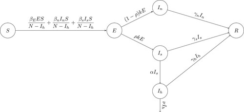
Table 1. State variables of the COVID-19 model (1(1) $\begin{array}{l}{\displaystyle S^{\prime }=-{\displaystyle \frac{{\beta }_{E}ES+{\beta }_n{I}_{n}S+{\beta }_s{I}_{s}S}{N-I_h}},}\\ {\displaystyle E^{\prime }={\displaystyle \frac{{\beta }_{E}ES+{\beta }_n{I}_{n}S+{\beta }_s{I}_{s}S}{N-I_h}}-kE,}\\ I_n^{\prime }=(1-\rho )kE-{\gamma }_n{I}_n,\\ I_s^{\prime }=\rho kE-(\alpha +{\gamma }_s)I_s,\\ I_h^{\prime }=\alpha I_s-({\gamma }_h+\nu )I_h,\\ R^{\prime }={\gamma }_n{I}_n+{\gamma }_s{I}_s+{\gamma }_h{I}_h.\end{array}$(1) ) and their definitions.

Variables	Definition
$S(t)$	Number of susceptible individuals at time t
$E(t)$	Number of individuals who are exposed to COVID-19 and are in their incubation period at time t
$I_n(t)$	Number of infectious individuals who are not tested and
	not showing any clinical COVID-19 symptoms at time t
$I_s(t)$	Number of infectious individuals are tested and showing clinical COVID-19 symptoms at time t
$I_h(t)$	Number of hospitalized individuals due to COVID-19 at time t
$R(t)$	Number of recovered individuals at time t

Table 2. Definition of the COVID-19 model parameters.

Parameter	Definition
${\beta }_E,{\beta }_n,{\beta }_s$	Transmission rate for exposed E, asymptomatic $I_n$, and symptomatic $I_s$ individuals
$q_E,q_n$	Relative infectiousness of exposed and non-symptomatic individuals
1/k	Incubation period
ρ	Proportion of individuals that undergo testing and test positive
	(Proportion of infected individuals that show COVID-19 symptoms)
${\gamma }_n,{\gamma }_s,{\gamma }_h$	Recovery rate for asymptomatic $I_n$, symptomatic $I_s$, and hospitalized $I_h$ individuals
α	Hospitalization rate of severely infected symptomatic $I_s$ individuals
ν	Disease induced mortality

We compute the reproduction number of (1(1) $\begin{array}{l}{\displaystyle S^{\prime }=-{\displaystyle \frac{{\beta }_{E}ES+{\beta }_n{I}_{n}S+{\beta }_s{I}_{s}S}{N-I_h}},}\\ {\displaystyle E^{\prime }={\displaystyle \frac{{\beta }_{E}ES+{\beta }_n{I}_{n}S+{\beta }_s{I}_{s}S}{N-I_h}}-kE,}\\ I_n^{\prime }=(1-\rho )kE-{\gamma }_n{I}_n,\\ I_s^{\prime }=\rho kE-(\alpha +{\gamma }_s)I_s,\\ I_h^{\prime }=\alpha I_s-({\gamma }_h+\nu )I_h,\\ R^{\prime }={\gamma }_n{I}_n+{\gamma }_s{I}_s+{\gamma }_h{I}_h.\end{array}$(1) ) to obtain ${\mathcal{R}}_0=\left({\displaystyle \frac{{\beta }_E}{k}+(1-\rho ){\displaystyle \frac{{\beta }_n}{{\gamma }_n}+\rho {\displaystyle \frac{{\beta }_s}{{\gamma }_s+\alpha }}}}\right){\displaystyle \frac{S(0)}{N(0)},}$where $N(0)=S(0)+E(0)+I_n(0)+I_s(0)+I_h(0)+R(0)$ is the initial total population size. The reproduction number consists of three terms, each of which corresponds to secondary cases produced by one type of infectious individuals. The first term is the number of secondary infections produced by exposed individuals in an entirely susceptible population during their lifespan as exposed, the second term is the number of secondary infections produced by asymptomatic and uncounted individuals in an entirely susceptible population during their lifespan as asymptomatic; finally, the third term corresponds to the number of secondary infections produced by symptomatic individuals during their lifespan as symptomatic and counted.

3. Identifiability analysis: can we uniquely estimate the model parameters?

In the literature, the term identifiability analysis is used to describe whether it is possible to uniquely recover model parameters from a given set of data. It is a crucial step in parameter estimation problem and is usually performed in two steps. The first step is the structural identifiability which is a theoretical property of the epidemic model. Structural identifiability explores whether the epidemic model is structured to reveal its parameters from the observations. Here we use the term observation to refer to continuous smooth output where the data is measured at the discrete time points. If a compartmental epidemic model is structurally unidentifiable, it means that different sets of parameters could produce the same output. Hence a structurally unidentifiable epidemic model should not be used to analyse epidemiological data or design intervention strategies. If an epidemic model is structurally identifiable, then the second step is the practical identifiability. Practical identifiability considers the actual epidemiological data which is contaminated with noise.

3.1. Structural identifiability analysis

To study the structural identifiability of the epidemic model, we represent the model (1(1) $\begin{array}{l}{\displaystyle S^{\prime }=-{\displaystyle \frac{{\beta }_{E}ES+{\beta }_n{I}_{n}S+{\beta }_s{I}_{s}S}{N-I_h}},}\\ {\displaystyle E^{\prime }={\displaystyle \frac{{\beta }_{E}ES+{\beta }_n{I}_{n}S+{\beta }_s{I}_{s}S}{N-I_h}}-kE,}\\ I_n^{\prime }=(1-\rho )kE-{\gamma }_n{I}_n,\\ I_s^{\prime }=\rho kE-(\alpha +{\gamma }_s)I_s,\\ I_h^{\prime }=\alpha I_s-({\gamma }_h+\nu )I_h,\\ R^{\prime }={\gamma }_n{I}_n+{\gamma }_s{I}_s+{\gamma }_h{I}_h.\end{array}$(1) ) in the following compact form: (2) ${\mathit{x}}^{\prime }(t)=f(\mathit{x},\mathit{p}),\mathit{x}(0)=x_0$(2) where $\mathit{x}$ denotes the state variables and $\mathit{p}$ denotes the parameters of the model of (1(1) $\begin{array}{l}{\displaystyle S^{\prime }=-{\displaystyle \frac{{\beta }_{E}ES+{\beta }_n{I}_{n}S+{\beta }_s{I}_{s}S}{N-I_h}},}\\ {\displaystyle E^{\prime }={\displaystyle \frac{{\beta }_{E}ES+{\beta }_n{I}_{n}S+{\beta }_s{I}_{s}S}{N-I_h}}-kE,}\\ I_n^{\prime }=(1-\rho )kE-{\gamma }_n{I}_n,\\ I_s^{\prime }=\rho kE-(\alpha +{\gamma }_s)I_s,\\ I_h^{\prime }=\alpha I_s-({\gamma }_h+\nu )I_h,\\ R^{\prime }={\gamma }_n{I}_n+{\gamma }_s{I}_s+{\gamma }_h{I}_h.\end{array}$(1) ). The observations, such as daily incidences and deaths, are functions of the state variables. Let $y_1(t)$ denote the daily incidences and $y_2(t)$ denote daily reported deaths, then in terms of model variables the observations take the following forms; (3) $y_1(t)=\rho kE\text{and}{y}_2(t)=\nu I_h$(3) In compact form, we denote the observations as $\mathit{y}(t)=(y_1(t),y_2(t))$ such that (4) $\mathit{y}(t)=\mathit{g}(\mathit{x},\mathit{p})=(\rho kE,\nu I_h).$(4) Structural identifiability determines whether the model (2(2) ${\mathit{x}}^{\prime }(t)=f(\mathit{x},\mathit{p}),\mathit{x}(0)=x_0$(2) ) is structured to reveal its parameters, $\mathit{p}$, from observations (4(4) $\mathit{y}(t)=\mathit{g}(\mathit{x},\mathit{p})=(\rho kE,\nu I_h).$(4) ). Structural identifiability is a theoretical result which considers the ‘perfect’ scenario assuming that observation is given continuously for all time and is noise free. A model is said to be structurally (uniquely) identifiable if all the parameters in $\mathit{p}$ can be recovered from the observations $\mathit{y}$. If even one parameter cannot be identified, the mode is said to be structurally unidentifiable. Several methods for determining structural identifiability have been introduced and studied widely [10,22,33]. Here, we will use the Differential Algebra approach to study the structural identifiability [22]. The goal of Differential Algebra approach is to eliminate the unobserved state variables using the system of differential equations in (2(2) ${\mathit{x}}^{\prime }(t)=f(\mathit{x},\mathit{p}),\mathit{x}(0)=x_0$(2) ) and to obtain input–output equations. We obtain the input–output equations of the model (1(1) $\begin{array}{l}{\displaystyle S^{\prime }=-{\displaystyle \frac{{\beta }_{E}ES+{\beta }_n{I}_{n}S+{\beta }_s{I}_{s}S}{N-I_h}},}\\ {\displaystyle E^{\prime }={\displaystyle \frac{{\beta }_{E}ES+{\beta }_n{I}_{n}S+{\beta }_s{I}_{s}S}{N-I_h}}-kE,}\\ I_n^{\prime }=(1-\rho )kE-{\gamma }_n{I}_n,\\ I_s^{\prime }=\rho kE-(\alpha +{\gamma }_s)I_s,\\ I_h^{\prime }=\alpha I_s-({\gamma }_h+\nu )I_h,\\ R^{\prime }={\gamma }_n{I}_n+{\gamma }_s{I}_s+{\gamma }_h{I}_h.\end{array}$(1) ) using the observations (3(3) $y_1(t)=\rho kE\text{and}{y}_2(t)=\nu I_h$(3) ), which consist of a couple of monic differential polynomials in the observed state variables and their derivatives. The coefficients of these polynomials are rational functions of the parameters of the model. We obtain the following input–output equations using DAISY [1]. (5) $\begin{array}{rl}& \frac{\mathrm{d}{y}_1}{\mathrm{d}t}-\frac{\mathrm{d}{y}_2}{\mathrm{d}t}\frac{{\beta }_{s}k\rho (\alpha -{\gamma }_n+{\gamma }_s)}{\alpha {\beta }_E\nu }-y_1\frac{-{\beta }_E{\gamma }_n+{\beta }_{n}k\rho -{\beta }_{n}k-{\beta }_{s}k\rho }{{\beta }_E}-y_2\frac{f_1(\mathit{p})}{\alpha {\beta }_E\nu }=0\end{array}$(5) (6) $\begin{array}{rl}& {\displaystyle \frac{{\mathrm{d}}^2{y}_2}{\mathrm{d}{t}^2}-{\displaystyle \frac{\mathrm{d}{y}_1}{\mathrm{d}t}{\displaystyle \frac{\alpha {\beta }_E\nu (\alpha +\nu +{\gamma }_s+{\gamma }_h)}{{\beta }_{s}k\rho (-\alpha +{\gamma }_n-{\gamma }_s)}+y_1{\displaystyle \frac{f_2(\mathit{p})}{{\beta }_{s}k\rho (-\alpha +{\gamma }_n-{\gamma }_s)}+y_2{\displaystyle \frac{f_3(\mathit{p})}{-\alpha +{\gamma }_n-{\gamma }_s}=0}}}}}\end{array}$(6) where $\begin{array}{rl}{f}_1(\mathit{p})& ={\beta }_{s}k\rho (\alpha \nu +\alpha {\gamma }_h-\nu {\gamma }_n+\nu {\gamma }_s-{\gamma }_n{\gamma }_h+{\gamma }_s{\gamma }_h)\\ f_2(\mathit{p})& =\alpha \nu (-\alpha {\beta }_E{\gamma }_n+\alpha {\beta }_{n}k\rho -\alpha {\beta }_{n}k-{\beta }_E\nu {\gamma }_n-{\beta }_E{\gamma }_n{\gamma }_s-{\beta }_E{\gamma }_n{\gamma }_h+{\beta }_n\nu k\rho \\ & -{\beta }_n\nu k+{\beta }_n{\gamma }_{s}k\rho -{\beta }_n{\gamma }_{s}k+{\beta }_{n}k{\gamma }_h\rho -{\beta }_{n}k{\gamma }_h-{\beta }_s\nu k\rho -{\beta }_s{\gamma }_{n}k\rho -{\beta }_{s}k{\gamma }_h\rho )\\ f_3(\mathit{p})& =\alpha {\nu }^2+2\alpha \nu {\gamma }_h+\alpha {\gamma }_h^2-{\nu }^2{\gamma }_n+{\nu }^2{\gamma }_s-2\nu {\gamma }_n{\gamma }_h+2\nu {\gamma }_s{\gamma }_h-{\gamma }_n{\gamma }_h^2+{\gamma }_s{\gamma }_h^2.\end{array}$ Input–output equations (5(5) $\begin{array}{rl}& \frac{\mathrm{d}{y}_1}{\mathrm{d}t}-\frac{\mathrm{d}{y}_2}{\mathrm{d}t}\frac{{\beta }_{s}k\rho (\alpha -{\gamma }_n+{\gamma }_s)}{\alpha {\beta }_E\nu }-y_1\frac{-{\beta }_E{\gamma }_n+{\beta }_{n}k\rho -{\beta }_{n}k-{\beta }_{s}k\rho }{{\beta }_E}-y_2\frac{f_1(\mathit{p})}{\alpha {\beta }_E\nu }=0\end{array}$(5) ) and (6(6) $\begin{array}{rl}& {\displaystyle \frac{{\mathrm{d}}^2{y}_2}{\mathrm{d}{t}^2}-{\displaystyle \frac{\mathrm{d}{y}_1}{\mathrm{d}t}{\displaystyle \frac{\alpha {\beta }_E\nu (\alpha +\nu +{\gamma }_s+{\gamma }_h)}{{\beta }_{s}k\rho (-\alpha +{\gamma }_n-{\gamma }_s)}+y_1{\displaystyle \frac{f_2(\mathit{p})}{{\beta }_{s}k\rho (-\alpha +{\gamma }_n-{\gamma }_s)}+y_2{\displaystyle \frac{f_3(\mathit{p})}{-\alpha +{\gamma }_n-{\gamma }_s}=0}}}}}\end{array}$(6) ) are differential algebraic polynomials of outputs $y_1$ and $y_2$ whose coefficients consist of model parameters. We say that the model (2(2) ${\mathit{x}}^{\prime }(t)=f(\mathit{x},\mathit{p}),\mathit{x}(0)=x_0$(2) ) is structurally identifiable if the mapping from parameter space to the coefficients of input–output equations (5(5) $\begin{array}{rl}& \frac{\mathrm{d}{y}_1}{\mathrm{d}t}-\frac{\mathrm{d}{y}_2}{\mathrm{d}t}\frac{{\beta }_{s}k\rho (\alpha -{\gamma }_n+{\gamma }_s)}{\alpha {\beta }_E\nu }-y_1\frac{-{\beta }_E{\gamma }_n+{\beta }_{n}k\rho -{\beta }_{n}k-{\beta }_{s}k\rho }{{\beta }_E}-y_2\frac{f_1(\mathit{p})}{\alpha {\beta }_E\nu }=0\end{array}$(5) ) and (6(6) $\begin{array}{rl}& {\displaystyle \frac{{\mathrm{d}}^2{y}_2}{\mathrm{d}{t}^2}-{\displaystyle \frac{\mathrm{d}{y}_1}{\mathrm{d}t}{\displaystyle \frac{\alpha {\beta }_E\nu (\alpha +\nu +{\gamma }_s+{\gamma }_h)}{{\beta }_{s}k\rho (-\alpha +{\gamma }_n-{\gamma }_s)}+y_1{\displaystyle \frac{f_2(\mathit{p})}{{\beta }_{s}k\rho (-\alpha +{\gamma }_n-{\gamma }_s)}+y_2{\displaystyle \frac{f_3(\mathit{p})}{-\alpha +{\gamma }_n-{\gamma }_s}=0}}}}}\end{array}$(6) ) are one-to-one [32,34]. Within differential algebra approach, we define the structural identifiability as follows [10,34]:

Definition 3.1

Let $c(\mathit{p})$ denote the coefficients of the input–output equations (5(5) $\begin{array}{rl}& \frac{\mathrm{d}{y}_1}{\mathrm{d}t}-\frac{\mathrm{d}{y}_2}{\mathrm{d}t}\frac{{\beta }_{s}k\rho (\alpha -{\gamma }_n+{\gamma }_s)}{\alpha {\beta }_E\nu }-y_1\frac{-{\beta }_E{\gamma }_n+{\beta }_{n}k\rho -{\beta }_{n}k-{\beta }_{s}k\rho }{{\beta }_E}-y_2\frac{f_1(\mathit{p})}{\alpha {\beta }_E\nu }=0\end{array}$(5) ) and (6(6) $\begin{array}{rl}& {\displaystyle \frac{{\mathrm{d}}^2{y}_2}{\mathrm{d}{t}^2}-{\displaystyle \frac{\mathrm{d}{y}_1}{\mathrm{d}t}{\displaystyle \frac{\alpha {\beta }_E\nu (\alpha +\nu +{\gamma }_s+{\gamma }_h)}{{\beta }_{s}k\rho (-\alpha +{\gamma }_n-{\gamma }_s)}+y_1{\displaystyle \frac{f_2(\mathit{p})}{{\beta }_{s}k\rho (-\alpha +{\gamma }_n-{\gamma }_s)}+y_2{\displaystyle \frac{f_3(\mathit{p})}{-\alpha +{\gamma }_n-{\gamma }_s}=0}}}}}\end{array}$(6) ). That is (7) $\begin{array}{rl}c(\mathit{p})& =(-{\displaystyle \frac{{\beta }_{s}k\rho (\alpha -{\gamma }_n+{\gamma }_s)}{\alpha {\beta }_E\nu },-{\displaystyle \frac{-{\beta }_E{\gamma }_n+{\beta }_{n}k\rho -{\beta }_{n}k-{\beta }_{s}k\rho }{{\beta }_E},{\displaystyle \frac{f_1(\mathit{p})}{\alpha {\beta }_E\nu },}}}\\ & -{\displaystyle \frac{\alpha {\beta }_E\nu (\alpha +\nu +{\gamma }_s+{\gamma }_h)}{{\beta }_{s}k\rho (-\alpha +{\gamma }_n-{\gamma }_s)},{\displaystyle \frac{f_2(\mathit{p})}{{\beta }_{s}k\rho (-\alpha +{\gamma }_n-{\gamma }_s)},{\displaystyle \frac{f_3(\mathit{p})}{-\alpha +{\gamma }_n-{\gamma }_s}}}})\end{array}$(7) with $\mathit{p}=({\beta }_E,{\beta }_n,{\beta }_s,k,\rho ,{\gamma }_n,{\gamma }_s,\alpha ,r,\nu )$ denoting the parameters of the model (1(1) $\begin{array}{l}{\displaystyle S^{\prime }=-{\displaystyle \frac{{\beta }_{E}ES+{\beta }_n{I}_{n}S+{\beta }_s{I}_{s}S}{N-I_h}},}\\ {\displaystyle E^{\prime }={\displaystyle \frac{{\beta }_{E}ES+{\beta }_n{I}_{n}S+{\beta }_s{I}_{s}S}{N-I_h}}-kE,}\\ I_n^{\prime }=(1-\rho )kE-{\gamma }_n{I}_n,\\ I_s^{\prime }=\rho kE-(\alpha +{\gamma }_s)I_s,\\ I_h^{\prime }=\alpha I_s-({\gamma }_h+\nu )I_h,\\ R^{\prime }={\gamma }_n{I}_n+{\gamma }_s{I}_s+{\gamma }_h{I}_h.\end{array}$(1) ). Then we say that the model (1(1) $\begin{array}{l}{\displaystyle S^{\prime }=-{\displaystyle \frac{{\beta }_{E}ES+{\beta }_n{I}_{n}S+{\beta }_s{I}_{s}S}{N-I_h}},}\\ {\displaystyle E^{\prime }={\displaystyle \frac{{\beta }_{E}ES+{\beta }_n{I}_{n}S+{\beta }_s{I}_{s}S}{N-I_h}}-kE,}\\ I_n^{\prime }=(1-\rho )kE-{\gamma }_n{I}_n,\\ I_s^{\prime }=\rho kE-(\alpha +{\gamma }_s)I_s,\\ I_h^{\prime }=\alpha I_s-({\gamma }_h+\nu )I_h,\\ R^{\prime }={\gamma }_n{I}_n+{\gamma }_s{I}_s+{\gamma }_h{I}_h.\end{array}$(1) ) is structured to reveal its parameters from the observations (3(3) $y_1(t)=\rho kE\text{and}{y}_2(t)=\nu I_h$(3) ) if and only if $c(\mathit{p})=c(\hat{\mathit{p}})⟹\mathit{p}=\hat{\mathit{p}}$

Following the definition of the structural identifiability, we set $\hat{\mathit{p}}=({\hat{\beta }}_E,{\hat{\beta }}_n,{\hat{\beta }}_s,\hat{k},\hat{\rho },{\hat{\gamma }}_n,{\hat{\gamma }}_s,\hat{\alpha },{\hat{\gamma }}_h,\hat{\nu })$. Then solving $c(\mathit{p})=c(\hat{\mathit{p}})$, we obtain the following parameter correlations: (8) $\begin{array}{rl}& {\displaystyle \frac{{\beta }_E}{{\hat{\beta }}_E}={\displaystyle \frac{{\beta }_{s}k\rho (\hat{\alpha }-{\gamma }_n+{\hat{\gamma }}_s)}{{\hat{\beta }}_s\hat{k}\hat{\rho }(\hat{\alpha }-{\hat{\gamma }}_n+{\hat{\gamma }}_s)}}}\\ & {\beta }_n(\rho -1)={\displaystyle \frac{{\beta }_s\rho }{{\hat{\beta }}_s\hat{k}\hat{\rho }(\hat{\alpha }-{\hat{\gamma }}_n+{\hat{\gamma }}_s)}(\hat{\alpha }{\hat{\beta }}_E{\gamma }_n-{\hat{\beta }}_E{\gamma }_n^2-\hat{\alpha }{\hat{\beta }}_E{\hat{\gamma }}_n+{\hat{\beta }}_E{\gamma }_n{\hat{\gamma }}_n+{\hat{\beta }}_E{\gamma }_n{\hat{\gamma }}_s-{\hat{\beta }}_E{\hat{\gamma }}_n{\hat{\gamma }}_s}\\ & -\hat{\alpha }{\hat{\beta }}_n\hat{k}+{\hat{\beta }}_n{\gamma }_n\hat{k}-{\hat{\beta }}_n{\hat{\gamma }}_s\hat{k}+\hat{\alpha }{\hat{\beta }}_n\hat{k}\hat{\rho }-{\hat{\beta }}_n{\gamma }_n\hat{k}\hat{\rho }+{\hat{\beta }}_s{\gamma }_n\hat{k}\hat{\rho }-{\hat{\beta }}_s{\hat{\gamma }}_n\hat{k}\hat{\rho }+{\hat{\beta }}_n{\hat{\gamma }}_s\hat{k}\hat{\rho })\\ & {\gamma }_s+\alpha ={\hat{\gamma }}_s+\hat{\alpha },\nu \alpha =\hat{\nu }\hat{\alpha },{\gamma }_h+\nu ={\hat{\gamma }}_h+\hat{\nu }\end{array}$(8) As it is evident in (8(8) $\begin{array}{rl}& {\displaystyle \frac{{\beta }_E}{{\hat{\beta }}_E}={\displaystyle \frac{{\beta }_{s}k\rho (\hat{\alpha }-{\gamma }_n+{\hat{\gamma }}_s)}{{\hat{\beta }}_s\hat{k}\hat{\rho }(\hat{\alpha }-{\hat{\gamma }}_n+{\hat{\gamma }}_s)}}}\\ & {\beta }_n(\rho -1)={\displaystyle \frac{{\beta }_s\rho }{{\hat{\beta }}_s\hat{k}\hat{\rho }(\hat{\alpha }-{\hat{\gamma }}_n+{\hat{\gamma }}_s)}(\hat{\alpha }{\hat{\beta }}_E{\gamma }_n-{\hat{\beta }}_E{\gamma }_n^2-\hat{\alpha }{\hat{\beta }}_E{\hat{\gamma }}_n+{\hat{\beta }}_E{\gamma }_n{\hat{\gamma }}_n+{\hat{\beta }}_E{\gamma }_n{\hat{\gamma }}_s-{\hat{\beta }}_E{\hat{\gamma }}_n{\hat{\gamma }}_s}\\ & -\hat{\alpha }{\hat{\beta }}_n\hat{k}+{\hat{\beta }}_n{\gamma }_n\hat{k}-{\hat{\beta }}_n{\hat{\gamma }}_s\hat{k}+\hat{\alpha }{\hat{\beta }}_n\hat{k}\hat{\rho }-{\hat{\beta }}_n{\gamma }_n\hat{k}\hat{\rho }+{\hat{\beta }}_s{\gamma }_n\hat{k}\hat{\rho }-{\hat{\beta }}_s{\hat{\gamma }}_n\hat{k}\hat{\rho }+{\hat{\beta }}_n{\hat{\gamma }}_s\hat{k}\hat{\rho })\\ & {\gamma }_s+\alpha ={\hat{\gamma }}_s+\hat{\alpha },\nu \alpha =\hat{\nu }\hat{\alpha },{\gamma }_h+\nu ={\hat{\gamma }}_h+\hat{\nu }\end{array}$(8) ), parameters of the model (1(1) $\begin{array}{l}{\displaystyle S^{\prime }=-{\displaystyle \frac{{\beta }_{E}ES+{\beta }_n{I}_{n}S+{\beta }_s{I}_{s}S}{N-I_h}},}\\ {\displaystyle E^{\prime }={\displaystyle \frac{{\beta }_{E}ES+{\beta }_n{I}_{n}S+{\beta }_s{I}_{s}S}{N-I_h}}-kE,}\\ I_n^{\prime }=(1-\rho )kE-{\gamma }_n{I}_n,\\ I_s^{\prime }=\rho kE-(\alpha +{\gamma }_s)I_s,\\ I_h^{\prime }=\alpha I_s-({\gamma }_h+\nu )I_h,\\ R^{\prime }={\gamma }_n{I}_n+{\gamma }_s{I}_s+{\gamma }_h{I}_h.\end{array}$(1) ) cannot be obtained from the observations of daily incidences and deaths. Some parameter combinations can be identified such as ${\gamma }_s+\alpha$ or $\nu \alpha$, but individual parameters ${\gamma }_s,\alpha$ or ν cannot be identified. Even if α is fixed to $\hat{\alpha }$ in (8(8) $\begin{array}{rl}& {\displaystyle \frac{{\beta }_E}{{\hat{\beta }}_E}={\displaystyle \frac{{\beta }_{s}k\rho (\hat{\alpha }-{\gamma }_n+{\hat{\gamma }}_s)}{{\hat{\beta }}_s\hat{k}\hat{\rho }(\hat{\alpha }-{\hat{\gamma }}_n+{\hat{\gamma }}_s)}}}\\ & {\beta }_n(\rho -1)={\displaystyle \frac{{\beta }_s\rho }{{\hat{\beta }}_s\hat{k}\hat{\rho }(\hat{\alpha }-{\hat{\gamma }}_n+{\hat{\gamma }}_s)}(\hat{\alpha }{\hat{\beta }}_E{\gamma }_n-{\hat{\beta }}_E{\gamma }_n^2-\hat{\alpha }{\hat{\beta }}_E{\hat{\gamma }}_n+{\hat{\beta }}_E{\gamma }_n{\hat{\gamma }}_n+{\hat{\beta }}_E{\gamma }_n{\hat{\gamma }}_s-{\hat{\beta }}_E{\hat{\gamma }}_n{\hat{\gamma }}_s}\\ & -\hat{\alpha }{\hat{\beta }}_n\hat{k}+{\hat{\beta }}_n{\gamma }_n\hat{k}-{\hat{\beta }}_n{\hat{\gamma }}_s\hat{k}+\hat{\alpha }{\hat{\beta }}_n\hat{k}\hat{\rho }-{\hat{\beta }}_n{\gamma }_n\hat{k}\hat{\rho }+{\hat{\beta }}_s{\gamma }_n\hat{k}\hat{\rho }-{\hat{\beta }}_s{\hat{\gamma }}_n\hat{k}\hat{\rho }+{\hat{\beta }}_n{\hat{\gamma }}_s\hat{k}\hat{\rho })\\ & {\gamma }_s+\alpha ={\hat{\gamma }}_s+\hat{\alpha },\nu \alpha =\hat{\nu }\hat{\alpha },{\gamma }_h+\nu ={\hat{\gamma }}_h+\hat{\nu }\end{array}$(8) ), then we can only obtain ${\gamma }_s={\hat{\gamma }}_s$, $\nu =\hat{\nu }$ and ${\gamma }_h={\hat{\gamma }}_h$, and the parameters ${\beta }_E,{\beta }_n,{\beta }_s,{\gamma }_n,k,\rho$ still cannot be identified. Thus we have proved the following Proposition 3.1.

Proposition 3.1

The parameters of the model (1(1) $\begin{array}{l}{\displaystyle S^{\prime }=-{\displaystyle \frac{{\beta }_{E}ES+{\beta }_n{I}_{n}S+{\beta }_s{I}_{s}S}{N-I_h}},}\\ {\displaystyle E^{\prime }={\displaystyle \frac{{\beta }_{E}ES+{\beta }_n{I}_{n}S+{\beta }_s{I}_{s}S}{N-I_h}}-kE,}\\ I_n^{\prime }=(1-\rho )kE-{\gamma }_n{I}_n,\\ I_s^{\prime }=\rho kE-(\alpha +{\gamma }_s)I_s,\\ I_h^{\prime }=\alpha I_s-({\gamma }_h+\nu )I_h,\\ R^{\prime }={\gamma }_n{I}_n+{\gamma }_s{I}_s+{\gamma }_h{I}_h.\end{array}$(1) ) are not structurally identifiable from the observations of daily incidences and deaths.

In this approach, we assume that the initial conditions are given and fixed. An important advantage of using Differential Algebra approach in structural identifiability analysis is that we obtain parameter correlations as in (8(8) $\begin{array}{rl}& {\displaystyle \frac{{\beta }_E}{{\hat{\beta }}_E}={\displaystyle \frac{{\beta }_{s}k\rho (\hat{\alpha }-{\gamma }_n+{\hat{\gamma }}_s)}{{\hat{\beta }}_s\hat{k}\hat{\rho }(\hat{\alpha }-{\hat{\gamma }}_n+{\hat{\gamma }}_s)}}}\\ & {\beta }_n(\rho -1)={\displaystyle \frac{{\beta }_s\rho }{{\hat{\beta }}_s\hat{k}\hat{\rho }(\hat{\alpha }-{\hat{\gamma }}_n+{\hat{\gamma }}_s)}(\hat{\alpha }{\hat{\beta }}_E{\gamma }_n-{\hat{\beta }}_E{\gamma }_n^2-\hat{\alpha }{\hat{\beta }}_E{\hat{\gamma }}_n+{\hat{\beta }}_E{\gamma }_n{\hat{\gamma }}_n+{\hat{\beta }}_E{\gamma }_n{\hat{\gamma }}_s-{\hat{\beta }}_E{\hat{\gamma }}_n{\hat{\gamma }}_s}\\ & -\hat{\alpha }{\hat{\beta }}_n\hat{k}+{\hat{\beta }}_n{\gamma }_n\hat{k}-{\hat{\beta }}_n{\hat{\gamma }}_s\hat{k}+\hat{\alpha }{\hat{\beta }}_n\hat{k}\hat{\rho }-{\hat{\beta }}_n{\gamma }_n\hat{k}\hat{\rho }+{\hat{\beta }}_s{\gamma }_n\hat{k}\hat{\rho }-{\hat{\beta }}_s{\hat{\gamma }}_n\hat{k}\hat{\rho }+{\hat{\beta }}_n{\hat{\gamma }}_s\hat{k}\hat{\rho })\\ & {\gamma }_s+\alpha ={\hat{\gamma }}_s+\hat{\alpha },\nu \alpha =\hat{\nu }\hat{\alpha },{\gamma }_h+\nu ={\hat{\gamma }}_h+\hat{\nu }\end{array}$(8) ). These parameter correlations are then used to obtain a structurally identifiable model [10,32]. However, the correlations in (8(8) $\begin{array}{rl}& {\displaystyle \frac{{\beta }_E}{{\hat{\beta }}_E}={\displaystyle \frac{{\beta }_{s}k\rho (\hat{\alpha }-{\gamma }_n+{\hat{\gamma }}_s)}{{\hat{\beta }}_s\hat{k}\hat{\rho }(\hat{\alpha }-{\hat{\gamma }}_n+{\hat{\gamma }}_s)}}}\\ & {\beta }_n(\rho -1)={\displaystyle \frac{{\beta }_s\rho }{{\hat{\beta }}_s\hat{k}\hat{\rho }(\hat{\alpha }-{\hat{\gamma }}_n+{\hat{\gamma }}_s)}(\hat{\alpha }{\hat{\beta }}_E{\gamma }_n-{\hat{\beta }}_E{\gamma }_n^2-\hat{\alpha }{\hat{\beta }}_E{\hat{\gamma }}_n+{\hat{\beta }}_E{\gamma }_n{\hat{\gamma }}_n+{\hat{\beta }}_E{\gamma }_n{\hat{\gamma }}_s-{\hat{\beta }}_E{\hat{\gamma }}_n{\hat{\gamma }}_s}\\ & -\hat{\alpha }{\hat{\beta }}_n\hat{k}+{\hat{\beta }}_n{\gamma }_n\hat{k}-{\hat{\beta }}_n{\hat{\gamma }}_s\hat{k}+\hat{\alpha }{\hat{\beta }}_n\hat{k}\hat{\rho }-{\hat{\beta }}_n{\gamma }_n\hat{k}\hat{\rho }+{\hat{\beta }}_s{\gamma }_n\hat{k}\hat{\rho }-{\hat{\beta }}_s{\hat{\gamma }}_n\hat{k}\hat{\rho }+{\hat{\beta }}_n{\hat{\gamma }}_s\hat{k}\hat{\rho })\\ & {\gamma }_s+\alpha ={\hat{\gamma }}_s+\hat{\alpha },\nu \alpha =\hat{\nu }\hat{\alpha },{\gamma }_h+\nu ={\hat{\gamma }}_h+\hat{\nu }\end{array}$(8) ) are highly complex. In an attempt to get a structurally identifiable model, we rewrite the parameter correlations into the following simpler forms; (9) $\begin{array}{rl}& {\displaystyle \frac{{\beta }_E}{{\hat{\beta }}_E}={\displaystyle \frac{{\beta }_{s}k\rho (\hat{\alpha }-{\gamma }_n+{\hat{\gamma }}_s)}{{\hat{\beta }}_s\hat{k}\hat{\rho }(\hat{\alpha }-{\hat{\gamma }}_n+{\hat{\gamma }}_s)}}}\\ & {\displaystyle \frac{{\beta }_n(\rho -1)}{{\beta }_s\rho }={\displaystyle \frac{{\hat{\beta }}_n(\hat{\rho }-1)}{{\hat{\beta }}_s\hat{\rho }}{\displaystyle \frac{(\hat{\alpha }-{\gamma }_n+{\hat{\gamma }}_s)}{(\hat{\alpha }-{\hat{\gamma }}_n+{\hat{\gamma }}_s)}+{\displaystyle \frac{{\hat{\beta }}_E}{{\hat{\beta }}_s\hat{k}\hat{\rho }}{\displaystyle \frac{(\hat{\alpha }-{\gamma }_n+{\hat{\gamma }}_s)}{(\hat{\alpha }-{\hat{\gamma }}_n+{\hat{\gamma }}_s)}({\gamma }_n-{\hat{\gamma }}_n)}}}}}\\ & +{\displaystyle \frac{1}{\hat{\alpha }-{\hat{\gamma }}_n+{\hat{\gamma }}_s}({\gamma }_n-{\hat{\gamma }}_n)}\\ & {\gamma }_s+\alpha ={\hat{\gamma }}_s+\hat{\alpha },\nu \alpha =\hat{\nu }\hat{\alpha },{\gamma }_h+\nu ={\hat{\gamma }}_h+\hat{\nu }\end{array}$(9) Next, we factor out ${\beta }_s$ from the incidences term in model (1(1) $\begin{array}{l}{\displaystyle S^{\prime }=-{\displaystyle \frac{{\beta }_{E}ES+{\beta }_n{I}_{n}S+{\beta }_s{I}_{s}S}{N-I_h}},}\\ {\displaystyle E^{\prime }={\displaystyle \frac{{\beta }_{E}ES+{\beta }_n{I}_{n}S+{\beta }_s{I}_{s}S}{N-I_h}}-kE,}\\ I_n^{\prime }=(1-\rho )kE-{\gamma }_n{I}_n,\\ I_s^{\prime }=\rho kE-(\alpha +{\gamma }_s)I_s,\\ I_h^{\prime }=\alpha I_s-({\gamma }_h+\nu )I_h,\\ R^{\prime }={\gamma }_n{I}_n+{\gamma }_s{I}_s+{\gamma }_h{I}_h.\end{array}$(1) ) as follows: ${\beta }_s{\displaystyle \frac{q_{E}ES+q_n{I}_{n}S+I_{s}S}{N-I_h}}$where $q_E={\displaystyle \frac{{\beta }_E}{{\beta }_s}}$ and $q_n={\displaystyle \frac{{\beta }_n}{{\beta }_s}}$. With this setting, if we fix parameter α at $\hat{\alpha }$, and ${\gamma }_n$ at ${\hat{\gamma }}_n$ then the parameter correlations in (9(9) $\begin{array}{rl}& {\displaystyle \frac{{\beta }_E}{{\hat{\beta }}_E}={\displaystyle \frac{{\beta }_{s}k\rho (\hat{\alpha }-{\gamma }_n+{\hat{\gamma }}_s)}{{\hat{\beta }}_s\hat{k}\hat{\rho }(\hat{\alpha }-{\hat{\gamma }}_n+{\hat{\gamma }}_s)}}}\\ & {\displaystyle \frac{{\beta }_n(\rho -1)}{{\beta }_s\rho }={\displaystyle \frac{{\hat{\beta }}_n(\hat{\rho }-1)}{{\hat{\beta }}_s\hat{\rho }}{\displaystyle \frac{(\hat{\alpha }-{\gamma }_n+{\hat{\gamma }}_s)}{(\hat{\alpha }-{\hat{\gamma }}_n+{\hat{\gamma }}_s)}+{\displaystyle \frac{{\hat{\beta }}_E}{{\hat{\beta }}_s\hat{k}\hat{\rho }}{\displaystyle \frac{(\hat{\alpha }-{\gamma }_n+{\hat{\gamma }}_s)}{(\hat{\alpha }-{\hat{\gamma }}_n+{\hat{\gamma }}_s)}({\gamma }_n-{\hat{\gamma }}_n)}}}}}\\ & +{\displaystyle \frac{1}{\hat{\alpha }-{\hat{\gamma }}_n+{\hat{\gamma }}_s}({\gamma }_n-{\hat{\gamma }}_n)}\\ & {\gamma }_s+\alpha ={\hat{\gamma }}_s+\hat{\alpha },\nu \alpha =\hat{\nu }\hat{\alpha },{\gamma }_h+\nu ={\hat{\gamma }}_h+\hat{\nu }\end{array}$(9) ) become (10) $\begin{array}{rl}{\displaystyle \frac{q_E}{k\rho }}& ={\displaystyle \frac{{\hat{q}}_E}{\hat{k}\hat{\rho }},{\displaystyle \frac{q_n(\rho -1)}{\rho }={\displaystyle \frac{{\hat{q}}_n(\hat{\rho }-1)}{\hat{\rho }},\alpha =\hat{\alpha },{\gamma }_n={\hat{\gamma }}_n,{\gamma }_s={\hat{\gamma }}_s,}}}\\ {\gamma }_h& ={\hat{\gamma }}_h,\nu =\hat{\nu }.\end{array}$(10) We can see from (10(10) $\begin{array}{rl}{\displaystyle \frac{q_E}{k\rho }}& ={\displaystyle \frac{{\hat{q}}_E}{\hat{k}\hat{\rho }},{\displaystyle \frac{q_n(\rho -1)}{\rho }={\displaystyle \frac{{\hat{q}}_n(\hat{\rho }-1)}{\hat{\rho }},\alpha =\hat{\alpha },{\gamma }_n={\hat{\gamma }}_n,{\gamma }_s={\hat{\gamma }}_s,}}}\\ {\gamma }_h& ={\hat{\gamma }}_h,\nu =\hat{\nu }.\end{array}$(10) ) that the parameters $\alpha ,{\gamma }_n,{\gamma }_s,{\gamma }_h$ and ν can be identified; parameter combinations ${\displaystyle \frac{q_E}{k\rho }}$ and ${\displaystyle \frac{q_n(\rho -1)}{\rho }}$ can be identified; but parameter ${\beta }_s$ cannot be identified. For instance, the parameter correlation ${\displaystyle \frac{q_E}{k\rho }}$ implies that infinitely many values of the parameters $q_E,k$ and ρ would generate the same output as long as the parameter relationship ${\displaystyle \frac{q_E}{k\rho }}$ remains constant at ${\displaystyle \frac{{\hat{q}}_E}{\hat{k}\hat{\rho }}}$. Same is true for parameters ρ and $q_n$ satisfying the relationship ${\displaystyle \frac{q_n(\rho -1)}{\rho }}$. In the view of these results, we obtain the following Proposition 3.2.

Proposition 3.2

If the parameters, $\alpha ,{\gamma }_n,k$ and ρ are fixed, then solving $c(\mathit{p})=c(\hat{\mathit{p}})$, we obtain $\begin{array}{rl}{q}_E& ={\hat{q}}_E,q_n={\hat{q}}_n,k=\hat{k},\rho =\hat{\rho },\alpha =\hat{\alpha },{\gamma }_n={\hat{\gamma }}_n,{\gamma }_s={\hat{\gamma }}_s,\\ {\gamma }_h& ={\hat{\gamma }}_h,\nu =\hat{\nu }.\end{array}$Since, ${\beta }_s$ still cannot be obtained we say that the model (1(1) $\begin{array}{l}{\displaystyle S^{\prime }=-{\displaystyle \frac{{\beta }_{E}ES+{\beta }_n{I}_{n}S+{\beta }_s{I}_{s}S}{N-I_h}},}\\ {\displaystyle E^{\prime }={\displaystyle \frac{{\beta }_{E}ES+{\beta }_n{I}_{n}S+{\beta }_s{I}_{s}S}{N-I_h}}-kE,}\\ I_n^{\prime }=(1-\rho )kE-{\gamma }_n{I}_n,\\ I_s^{\prime }=\rho kE-(\alpha +{\gamma }_s)I_s,\\ I_h^{\prime }=\alpha I_s-({\gamma }_h+\nu )I_h,\\ R^{\prime }={\gamma }_n{I}_n+{\gamma }_s{I}_s+{\gamma }_h{I}_h.\end{array}$(1) ) is structurally unidentifiable from the observations of daily incidences and deaths.

Remark 3.1

The model (1(1) $\begin{array}{l}{\displaystyle S^{\prime }=-{\displaystyle \frac{{\beta }_{E}ES+{\beta }_n{I}_{n}S+{\beta }_s{I}_{s}S}{N-I_h}},}\\ {\displaystyle E^{\prime }={\displaystyle \frac{{\beta }_{E}ES+{\beta }_n{I}_{n}S+{\beta }_s{I}_{s}S}{N-I_h}}-kE,}\\ I_n^{\prime }=(1-\rho )kE-{\gamma }_n{I}_n,\\ I_s^{\prime }=\rho kE-(\alpha +{\gamma }_s)I_s,\\ I_h^{\prime }=\alpha I_s-({\gamma }_h+\nu )I_h,\\ R^{\prime }={\gamma }_n{I}_n+{\gamma }_s{I}_s+{\gamma }_h{I}_h.\end{array}$(1) ) is not structurally identifiable, because the parameter ${\beta }_s$ does not appear in the parameter relations in (10(10) $\begin{array}{rl}{\displaystyle \frac{q_E}{k\rho }}& ={\displaystyle \frac{{\hat{q}}_E}{\hat{k}\hat{\rho }},{\displaystyle \frac{q_n(\rho -1)}{\rho }={\displaystyle \frac{{\hat{q}}_n(\hat{\rho }-1)}{\hat{\rho }},\alpha =\hat{\alpha },{\gamma }_n={\hat{\gamma }}_n,{\gamma }_s={\hat{\gamma }}_s,}}}\\ {\gamma }_h& ={\hat{\gamma }}_h,\nu =\hat{\nu }.\end{array}$(10) ). But all the other parameters are identifiable. We use the following strategy in an attempt to make ${\beta }_s$ an identifiable parameter; we use the basic reproduction number ${\mathcal{R}}_0$ to determine the infection rate ${\beta }_s$ as ${\beta }_s={\mathcal{R}}_0/\left({\displaystyle \frac{q_E}{k}+(1-\rho ){\displaystyle \frac{q_n}{{\gamma }_n}+\rho {\displaystyle \frac{1}{{\gamma }_s+\alpha }}}}\right){\displaystyle \frac{S(0)}{N(0)}.}$If we use estimate from the literature of ${\mathcal{R}}_0$, and fix ${\mathcal{R}}_0$ at that value, then ${\beta }_s$ will be identifiable as well.

3.1.1. Structural identifiability of COVID-19 epidemic models

We take this opportunity and study the structural identifiability of some COVID-19 models. Several models are proposed within the last year for COVID-19 infection and most of these models, including our model (1(1) $\begin{array}{l}{\displaystyle S^{\prime }=-{\displaystyle \frac{{\beta }_{E}ES+{\beta }_n{I}_{n}S+{\beta }_s{I}_{s}S}{N-I_h}},}\\ {\displaystyle E^{\prime }={\displaystyle \frac{{\beta }_{E}ES+{\beta }_n{I}_{n}S+{\beta }_s{I}_{s}S}{N-I_h}}-kE,}\\ I_n^{\prime }=(1-\rho )kE-{\gamma }_n{I}_n,\\ I_s^{\prime }=\rho kE-(\alpha +{\gamma }_s)I_s,\\ I_h^{\prime }=\alpha I_s-({\gamma }_h+\nu )I_h,\\ R^{\prime }={\gamma }_n{I}_n+{\gamma }_s{I}_s+{\gamma }_h{I}_h.\end{array}$(1) ), are extensions of the following Kermack–McKendrick type SEIR epidemic model without human demography. (M$_1$) $\mathbf{M}\mathbf{o}\mathbf{d}\mathbf{e}\mathbf{l}\mathbf{1}\mathbf{(}{\mathbf{M}}_{\mathbf{1}}\mathbf{)}\mathbf{:}\{\begin{array}{l}{\displaystyle S^{\prime }=-\frac{{\beta }_{E}ES+\beta IS}{N},}\\ {\displaystyle E^{\prime }=\frac{{\beta }_{E}ES+\beta IS}{N}-kE,}\\ I^{\prime }=kE-(\nu +\gamma )I,\\ R^{\prime }=\gamma I.\end{array}$(M$_1$) As before we assume that the observations are daily incidences and COVID-19 deaths. In terms of the state variables of the model (M₁(M$_1$) $\mathbf{M}\mathbf{o}\mathbf{d}\mathbf{e}\mathbf{l}\mathbf{1}\mathbf{(}{\mathbf{M}}_{\mathbf{1}}\mathbf{)}\mathbf{:}\{\begin{array}{l}{\displaystyle S^{\prime }=-\frac{{\beta }_{E}ES+\beta IS}{N},}\\ {\displaystyle E^{\prime }=\frac{{\beta }_{E}ES+\beta IS}{N}-kE,}\\ I^{\prime }=kE-(\nu +\gamma )I,\\ R^{\prime }=\gamma I.\end{array}$(M$_1$) ), observations becomes $y_1(t)=kE,y_2(t)=\nu I.$We have determined the input–output equations of the model M₁(M$_1$) $\mathbf{M}\mathbf{o}\mathbf{d}\mathbf{e}\mathbf{l}\mathbf{1}\mathbf{(}{\mathbf{M}}_{\mathbf{1}}\mathbf{)}\mathbf{:}\{\begin{array}{l}{\displaystyle S^{\prime }=-\frac{{\beta }_{E}ES+\beta IS}{N},}\\ {\displaystyle E^{\prime }=\frac{{\beta }_{E}ES+\beta IS}{N}-kE,}\\ I^{\prime }=kE-(\nu +\gamma )I,\\ R^{\prime }=\gamma I.\end{array}$(M$_1$) and show that it is structurally (globally) identifiable and obtain the following result (see Appendix for details).

Proposition 3.3

The model (M₁(M$_1$) $\mathbf{M}\mathbf{o}\mathbf{d}\mathbf{e}\mathbf{l}\mathbf{1}\mathbf{(}{\mathbf{M}}_{\mathbf{1}}\mathbf{)}\mathbf{:}\{\begin{array}{l}{\displaystyle S^{\prime }=-\frac{{\beta }_{E}ES+\beta IS}{N},}\\ {\displaystyle E^{\prime }=\frac{{\beta }_{E}ES+\beta IS}{N}-kE,}\\ I^{\prime }=kE-(\nu +\gamma )I,\\ R^{\prime }=\gamma I.\end{array}$(M$_1$) ) is structurally identifiable from the observations of daily incidences $y_1(t)=kE$, and deaths $y_2(t)=\nu I$.

In Proposition 3.3, it is assumed that all new incidences, kE are observed. However, this is not the case in reality. A key feature of COVID-19 cases is that majority of new infections are generated by individuals who do not show any clinical symptoms of COVID-19. A big portion of these asymptomatic individuals will remain undetected and only some might be detected through random testing or contact tracing. This leads to the fact that only the fraction of new incidences are reported. We continue with the identifiability analysis assuming that only fractions of daily incidences are observed, that is if we set $y_1(t)=\rho kE$ for $0<\rho <1$ then the parameter correlations for model (M₁(M$_1$) $\mathbf{M}\mathbf{o}\mathbf{d}\mathbf{e}\mathbf{l}\mathbf{1}\mathbf{(}{\mathbf{M}}_{\mathbf{1}}\mathbf{)}\mathbf{:}\{\begin{array}{l}{\displaystyle S^{\prime }=-\frac{{\beta }_{E}ES+\beta IS}{N},}\\ {\displaystyle E^{\prime }=\frac{{\beta }_{E}ES+\beta IS}{N}-kE,}\\ I^{\prime }=kE-(\nu +\gamma )I,\\ R^{\prime }=\gamma I.\end{array}$(M$_1$) ) become (12) ${\displaystyle \frac{{\beta }_E}{\beta }={\displaystyle \frac{{\hat{\beta }}_E}{\hat{\beta }},\nu \beta =\hat{\nu }\hat{\beta },\rho \beta =\hat{\rho }\hat{\beta },\gamma \beta +\hat{\nu }\beta =\hat{\gamma }\hat{\beta }+\hat{\nu }\hat{\beta },k=\hat{k}}}$(12) Assuming a much realistic scenario that only a fraction of actual incidences can be observed, makes the simple SEIR model unidentifiable. Thus we have obtained the following result for model (M₁(M$_1$) $\mathbf{M}\mathbf{o}\mathbf{d}\mathbf{e}\mathbf{l}\mathbf{1}\mathbf{(}{\mathbf{M}}_{\mathbf{1}}\mathbf{)}\mathbf{:}\{\begin{array}{l}{\displaystyle S^{\prime }=-\frac{{\beta }_{E}ES+\beta IS}{N},}\\ {\displaystyle E^{\prime }=\frac{{\beta }_{E}ES+\beta IS}{N}-kE,}\\ I^{\prime }=kE-(\nu +\gamma )I,\\ R^{\prime }=\gamma I.\end{array}$(M$_1$) ).

Proposition 3.4

The model (M₁(M$_1$) $\mathbf{M}\mathbf{o}\mathbf{d}\mathbf{e}\mathbf{l}\mathbf{1}\mathbf{(}{\mathbf{M}}_{\mathbf{1}}\mathbf{)}\mathbf{:}\{\begin{array}{l}{\displaystyle S^{\prime }=-\frac{{\beta }_{E}ES+\beta IS}{N},}\\ {\displaystyle E^{\prime }=\frac{{\beta }_{E}ES+\beta IS}{N}-kE,}\\ I^{\prime }=kE-(\nu +\gamma )I,\\ R^{\prime }=\gamma I.\end{array}$(M$_1$) ) with a fraction of observed cases is not structurally identifiable from the observations of daily incidences, $y_1(t)=\rho kE$, and deaths $y_2(t)=\nu I$.

Remark 3.2

From parameter correlations (11(12) ${\displaystyle \frac{{\beta }_E}{\beta }={\displaystyle \frac{{\hat{\beta }}_E}{\hat{\beta }},\nu \beta =\hat{\nu }\hat{\beta },\rho \beta =\hat{\rho }\hat{\beta },\gamma \beta +\hat{\nu }\beta =\hat{\gamma }\hat{\beta }+\hat{\nu }\hat{\beta },k=\hat{k}}}$(12) ), we see that if we set $\rho =\hat{\rho }$, that is if we assume that the fraction of the incidences being reported daily is known, then the model (M₁(M$_1$) $\mathbf{M}\mathbf{o}\mathbf{d}\mathbf{e}\mathbf{l}\mathbf{1}\mathbf{(}{\mathbf{M}}_{\mathbf{1}}\mathbf{)}\mathbf{:}\{\begin{array}{l}{\displaystyle S^{\prime }=-\frac{{\beta }_{E}ES+\beta IS}{N},}\\ {\displaystyle E^{\prime }=\frac{{\beta }_{E}ES+\beta IS}{N}-kE,}\\ I^{\prime }=kE-(\nu +\gamma )I,\\ R^{\prime }=\gamma I.\end{array}$(M$_1$) ) becomes structurally identifiable from daily incidences and deaths.

The next model, we will study is the one where infected class I is further divided into two subclasses, as asymptomatic individuals $I_n$ and symptomatic individuals $I_s$. Then we obtain the following model: (M$_2$) $\mathbf{M}\mathbf{o}\mathbf{d}\mathbf{e}\mathbf{l}\mathbf{2}\mathbf{(}{\mathbf{M}}_{\mathbf{2}}\mathbf{)}\mathbf{:}\{\begin{array}{l}{\displaystyle S^{\prime }=-\frac{{\beta }_{E}ES+{\beta }_n{I}_{n}S+{\beta }_s{I}_{s}S}{N},}\\ {\displaystyle E^{\prime }=\frac{{\beta }_{E}ES+{\beta }_n{I}_{n}S+{\beta }_s{I}_{s}S}{N}-kE,}\\ I_n^{\prime }=(1-\rho )kE-{\gamma }_n{I}_n,\\ I_s^{\prime }=\rho kE-(\nu +{\gamma }_s)I_s,\\ R^{\prime }={\gamma }_n{I}_n+{\gamma }_s{I}_s.\end{array}$(M$_2$) In this model, we assume that all the infected individuals who are showing symptoms are getting tested. That is for this model (M₂(M$_2$) $\mathbf{M}\mathbf{o}\mathbf{d}\mathbf{e}\mathbf{l}\mathbf{2}\mathbf{(}{\mathbf{M}}_{\mathbf{2}}\mathbf{)}\mathbf{:}\{\begin{array}{l}{\displaystyle S^{\prime }=-\frac{{\beta }_{E}ES+{\beta }_n{I}_{n}S+{\beta }_s{I}_{s}S}{N},}\\ {\displaystyle E^{\prime }=\frac{{\beta }_{E}ES+{\beta }_n{I}_{n}S+{\beta }_s{I}_{s}S}{N}-kE,}\\ I_n^{\prime }=(1-\rho )kE-{\gamma }_n{I}_n,\\ I_s^{\prime }=\rho kE-(\nu +{\gamma }_s)I_s,\\ R^{\prime }={\gamma }_n{I}_n+{\gamma }_s{I}_s.\end{array}$(M$_2$) ), observations of daily incidences and deaths take the form $y_1(t)=\rho kE,y_2(t)=\nu I_s$. Determining the input–output equations and then solving $c(\mathit{p})=c(\hat{\mathit{p}})$, gives the following parameter correlations; (14) $\frac{{\beta }_E}{{\beta }_s\rho }=\frac{{\hat{\beta }}_E}{{\hat{\beta }}_s\hat{\rho }}\frac{{\beta }_n(1-\rho )}{{\beta }_s\rho }=\frac{{\hat{\beta }}_n(1-\hat{\rho })}{{\hat{\beta }}_s\hat{\rho }}\frac{{\gamma }_n}{\nu }=\frac{{\hat{\gamma }}_n}{\hat{\nu }}\frac{{\gamma }_s}{\nu }=\frac{{\hat{\gamma }}_s}{\hat{\nu }}\frac{k}{\nu }=\frac{\hat{k}}{\hat{\nu }}$(14)

Proposition 3.5

The model (M₂(M$_2$) $\mathbf{M}\mathbf{o}\mathbf{d}\mathbf{e}\mathbf{l}\mathbf{2}\mathbf{(}{\mathbf{M}}_{\mathbf{2}}\mathbf{)}\mathbf{:}\{\begin{array}{l}{\displaystyle S^{\prime }=-\frac{{\beta }_{E}ES+{\beta }_n{I}_{n}S+{\beta }_s{I}_{s}S}{N},}\\ {\displaystyle E^{\prime }=\frac{{\beta }_{E}ES+{\beta }_n{I}_{n}S+{\beta }_s{I}_{s}S}{N}-kE,}\\ I_n^{\prime }=(1-\rho )kE-{\gamma }_n{I}_n,\\ I_s^{\prime }=\rho kE-(\nu +{\gamma }_s)I_s,\\ R^{\prime }={\gamma }_n{I}_n+{\gamma }_s{I}_s.\end{array}$(M$_2$) ) is not structurally identifiable from the observations of daily incidences, $y_1(t)=\rho kE$, and deaths $y_2(t)=\nu I_s$.

If we assume both the incubation period and the fraction of infected individuals who are showing symptoms are known, and set $k=\hat{k}$, $\rho =\hat{\rho }$. Furthermore, if we set as before, $q_E={\displaystyle \frac{{\beta }_E}{{\beta }_s}}$ and $q_n={\displaystyle \frac{{\beta }_n}{{\beta }_s}}$, then the following parameters of the model (M₂(M$_2$) $\mathbf{M}\mathbf{o}\mathbf{d}\mathbf{e}\mathbf{l}\mathbf{2}\mathbf{(}{\mathbf{M}}_{\mathbf{2}}\mathbf{)}\mathbf{:}\{\begin{array}{l}{\displaystyle S^{\prime }=-\frac{{\beta }_{E}ES+{\beta }_n{I}_{n}S+{\beta }_s{I}_{s}S}{N},}\\ {\displaystyle E^{\prime }=\frac{{\beta }_{E}ES+{\beta }_n{I}_{n}S+{\beta }_s{I}_{s}S}{N}-kE,}\\ I_n^{\prime }=(1-\rho )kE-{\gamma }_n{I}_n,\\ I_s^{\prime }=\rho kE-(\nu +{\gamma }_s)I_s,\\ R^{\prime }={\gamma }_n{I}_n+{\gamma }_s{I}_s.\end{array}$(M$_2$) ) can be identified, $q_E={\hat{q}}_E,q_n={\hat{q}}_n,{\gamma }_n={\hat{\gamma }}_n,{\gamma }_s={\hat{\gamma }}_s,\nu =\hat{\nu },\rho =\hat{\rho },k=\hat{k}$Since all the parameter but ${\beta }_s$ can be identified. We use the same strategy as before and determine ${\beta }_s$ from the basic reproduction number of the model (M₂(M$_2$) $\mathbf{M}\mathbf{o}\mathbf{d}\mathbf{e}\mathbf{l}\mathbf{2}\mathbf{(}{\mathbf{M}}_{\mathbf{2}}\mathbf{)}\mathbf{:}\{\begin{array}{l}{\displaystyle S^{\prime }=-\frac{{\beta }_{E}ES+{\beta }_n{I}_{n}S+{\beta }_s{I}_{s}S}{N},}\\ {\displaystyle E^{\prime }=\frac{{\beta }_{E}ES+{\beta }_n{I}_{n}S+{\beta }_s{I}_{s}S}{N}-kE,}\\ I_n^{\prime }=(1-\rho )kE-{\gamma }_n{I}_n,\\ I_s^{\prime }=\rho kE-(\nu +{\gamma }_s)I_s,\\ R^{\prime }={\gamma }_n{I}_n+{\gamma }_s{I}_s.\end{array}$(M$_2$) ). We summarize the results in the following proposition.

Proposition 3.6

If the parameters k and ρ are fixed, then $q_E,q_n,{\gamma }_n,{\gamma }_s$ and ν can be identified. But the model (M₂(M$_2$) $\mathbf{M}\mathbf{o}\mathbf{d}\mathbf{e}\mathbf{l}\mathbf{2}\mathbf{(}{\mathbf{M}}_{\mathbf{2}}\mathbf{)}\mathbf{:}\{\begin{array}{l}{\displaystyle S^{\prime }=-\frac{{\beta }_{E}ES+{\beta }_n{I}_{n}S+{\beta }_s{I}_{s}S}{N},}\\ {\displaystyle E^{\prime }=\frac{{\beta }_{E}ES+{\beta }_n{I}_{n}S+{\beta }_s{I}_{s}S}{N}-kE,}\\ I_n^{\prime }=(1-\rho )kE-{\gamma }_n{I}_n,\\ I_s^{\prime }=\rho kE-(\nu +{\gamma }_s)I_s,\\ R^{\prime }={\gamma }_n{I}_n+{\gamma }_s{I}_s.\end{array}$(M$_2$) ) remains structurally unidentifiable from the observations of daily incidences and deaths, since ${\beta }_s$ cannot be identified.

However, the infection rate ${\beta }_s$ can be determined from the identifiable model parameters through basic reproduction number ${\mathcal{R}}_0$, ${\mathcal{R}}_0={\beta }_s\left({\displaystyle \frac{q_E}{k}+(1-\rho ){\displaystyle \frac{q_n}{{\gamma }_n}+\rho {\displaystyle \frac{1}{\nu +{\gamma }_s}}}}\right){\displaystyle \frac{S(0)}{N(0)}.}$

Our intention for considering models (M₁(M$_1$) $\mathbf{M}\mathbf{o}\mathbf{d}\mathbf{e}\mathbf{l}\mathbf{1}\mathbf{(}{\mathbf{M}}_{\mathbf{1}}\mathbf{)}\mathbf{:}\{\begin{array}{l}{\displaystyle S^{\prime }=-\frac{{\beta }_{E}ES+\beta IS}{N},}\\ {\displaystyle E^{\prime }=\frac{{\beta }_{E}ES+\beta IS}{N}-kE,}\\ I^{\prime }=kE-(\nu +\gamma )I,\\ R^{\prime }=\gamma I.\end{array}$(M$_1$) ) and (M₂(M$_2$) $\mathbf{M}\mathbf{o}\mathbf{d}\mathbf{e}\mathbf{l}\mathbf{2}\mathbf{(}{\mathbf{M}}_{\mathbf{2}}\mathbf{)}\mathbf{:}\{\begin{array}{l}{\displaystyle S^{\prime }=-\frac{{\beta }_{E}ES+{\beta }_n{I}_{n}S+{\beta }_s{I}_{s}S}{N},}\\ {\displaystyle E^{\prime }=\frac{{\beta }_{E}ES+{\beta }_n{I}_{n}S+{\beta }_s{I}_{s}S}{N}-kE,}\\ I_n^{\prime }=(1-\rho )kE-{\gamma }_n{I}_n,\\ I_s^{\prime }=\rho kE-(\nu +{\gamma }_s)I_s,\\ R^{\prime }={\gamma }_n{I}_n+{\gamma }_s{I}_s.\end{array}$(M$_2$) ) is to find the most complex COVID-19 model which is intrinsically identifiable, that is identifiable without any restrictions on the parameters. It is worth mentioning that the models (M₁(M$_1$) $\mathbf{M}\mathbf{o}\mathbf{d}\mathbf{e}\mathbf{l}\mathbf{1}\mathbf{(}{\mathbf{M}}_{\mathbf{1}}\mathbf{)}\mathbf{:}\{\begin{array}{l}{\displaystyle S^{\prime }=-\frac{{\beta }_{E}ES+\beta IS}{N},}\\ {\displaystyle E^{\prime }=\frac{{\beta }_{E}ES+\beta IS}{N}-kE,}\\ I^{\prime }=kE-(\nu +\gamma )I,\\ R^{\prime }=\gamma I.\end{array}$(M$_1$) ), (M₂(M$_2$) $\mathbf{M}\mathbf{o}\mathbf{d}\mathbf{e}\mathbf{l}\mathbf{2}\mathbf{(}{\mathbf{M}}_{\mathbf{2}}\mathbf{)}\mathbf{:}\{\begin{array}{l}{\displaystyle S^{\prime }=-\frac{{\beta }_{E}ES+{\beta }_n{I}_{n}S+{\beta }_s{I}_{s}S}{N},}\\ {\displaystyle E^{\prime }=\frac{{\beta }_{E}ES+{\beta }_n{I}_{n}S+{\beta }_s{I}_{s}S}{N}-kE,}\\ I_n^{\prime }=(1-\rho )kE-{\gamma }_n{I}_n,\\ I_s^{\prime }=\rho kE-(\nu +{\gamma }_s)I_s,\\ R^{\prime }={\gamma }_n{I}_n+{\gamma }_s{I}_s.\end{array}$(M$_2$) ) and (1(1) $\begin{array}{l}{\displaystyle S^{\prime }=-{\displaystyle \frac{{\beta }_{E}ES+{\beta }_n{I}_{n}S+{\beta }_s{I}_{s}S}{N-I_h}},}\\ {\displaystyle E^{\prime }={\displaystyle \frac{{\beta }_{E}ES+{\beta }_n{I}_{n}S+{\beta }_s{I}_{s}S}{N-I_h}}-kE,}\\ I_n^{\prime }=(1-\rho )kE-{\gamma }_n{I}_n,\\ I_s^{\prime }=\rho kE-(\alpha +{\gamma }_s)I_s,\\ I_h^{\prime }=\alpha I_s-({\gamma }_h+\nu )I_h,\\ R^{\prime }={\gamma }_n{I}_n+{\gamma }_s{I}_s+{\gamma }_h{I}_h.\end{array}$(1) ) are nested models. Model (M₁(M$_1$) $\mathbf{M}\mathbf{o}\mathbf{d}\mathbf{e}\mathbf{l}\mathbf{1}\mathbf{(}{\mathbf{M}}_{\mathbf{1}}\mathbf{)}\mathbf{:}\{\begin{array}{l}{\displaystyle S^{\prime }=-\frac{{\beta }_{E}ES+\beta IS}{N},}\\ {\displaystyle E^{\prime }=\frac{{\beta }_{E}ES+\beta IS}{N}-kE,}\\ I^{\prime }=kE-(\nu +\gamma )I,\\ R^{\prime }=\gamma I.\end{array}$(M$_1$) ) is nested in model (M₂(M$_2$) $\mathbf{M}\mathbf{o}\mathbf{d}\mathbf{e}\mathbf{l}\mathbf{2}\mathbf{(}{\mathbf{M}}_{\mathbf{2}}\mathbf{)}\mathbf{:}\{\begin{array}{l}{\displaystyle S^{\prime }=-\frac{{\beta }_{E}ES+{\beta }_n{I}_{n}S+{\beta }_s{I}_{s}S}{N},}\\ {\displaystyle E^{\prime }=\frac{{\beta }_{E}ES+{\beta }_n{I}_{n}S+{\beta }_s{I}_{s}S}{N}-kE,}\\ I_n^{\prime }=(1-\rho )kE-{\gamma }_n{I}_n,\\ I_s^{\prime }=\rho kE-(\nu +{\gamma }_s)I_s,\\ R^{\prime }={\gamma }_n{I}_n+{\gamma }_s{I}_s.\end{array}$(M$_2$) ), and model (M₂(M$_2$) $\mathbf{M}\mathbf{o}\mathbf{d}\mathbf{e}\mathbf{l}\mathbf{2}\mathbf{(}{\mathbf{M}}_{\mathbf{2}}\mathbf{)}\mathbf{:}\{\begin{array}{l}{\displaystyle S^{\prime }=-\frac{{\beta }_{E}ES+{\beta }_n{I}_{n}S+{\beta }_s{I}_{s}S}{N},}\\ {\displaystyle E^{\prime }=\frac{{\beta }_{E}ES+{\beta }_n{I}_{n}S+{\beta }_s{I}_{s}S}{N}-kE,}\\ I_n^{\prime }=(1-\rho )kE-{\gamma }_n{I}_n,\\ I_s^{\prime }=\rho kE-(\nu +{\gamma }_s)I_s,\\ R^{\prime }={\gamma }_n{I}_n+{\gamma }_s{I}_s.\end{array}$(M$_2$) ) is nested in (1(1) $\begin{array}{l}{\displaystyle S^{\prime }=-{\displaystyle \frac{{\beta }_{E}ES+{\beta }_n{I}_{n}S+{\beta }_s{I}_{s}S}{N-I_h}},}\\ {\displaystyle E^{\prime }={\displaystyle \frac{{\beta }_{E}ES+{\beta }_n{I}_{n}S+{\beta }_s{I}_{s}S}{N-I_h}}-kE,}\\ I_n^{\prime }=(1-\rho )kE-{\gamma }_n{I}_n,\\ I_s^{\prime }=\rho kE-(\alpha +{\gamma }_s)I_s,\\ I_h^{\prime }=\alpha I_s-({\gamma }_h+\nu )I_h,\\ R^{\prime }={\gamma }_n{I}_n+{\gamma }_s{I}_s+{\gamma }_h{I}_h.\end{array}$(1) ). The simplest model (M₁(M$_1$) $\mathbf{M}\mathbf{o}\mathbf{d}\mathbf{e}\mathbf{l}\mathbf{1}\mathbf{(}{\mathbf{M}}_{\mathbf{1}}\mathbf{)}\mathbf{:}\{\begin{array}{l}{\displaystyle S^{\prime }=-\frac{{\beta }_{E}ES+\beta IS}{N},}\\ {\displaystyle E^{\prime }=\frac{{\beta }_{E}ES+\beta IS}{N}-kE,}\\ I^{\prime }=kE-(\nu +\gamma )I,\\ R^{\prime }=\gamma I.\end{array}$(M$_1$) ) is the only structurally identifiable model from the observations of daily incidences and casualties. As the model gets more complex as we increase the number of infectious classes in an attempt to capture the transmission dynamics of the COVID-19 infection, the epidemic model becomes unidentifiable.

3.2. Parameter estimation

We obtain the parameter estimates of the model (1(1) $\begin{array}{l}{\displaystyle S^{\prime }=-{\displaystyle \frac{{\beta }_{E}ES+{\beta }_n{I}_{n}S+{\beta }_s{I}_{s}S}{N-I_h}},}\\ {\displaystyle E^{\prime }={\displaystyle \frac{{\beta }_{E}ES+{\beta }_n{I}_{n}S+{\beta }_s{I}_{s}S}{N-I_h}}-kE,}\\ I_n^{\prime }=(1-\rho )kE-{\gamma }_n{I}_n,\\ I_s^{\prime }=\rho kE-(\alpha +{\gamma }_s)I_s,\\ I_h^{\prime }=\alpha I_s-({\gamma }_h+\nu )I_h,\\ R^{\prime }={\gamma }_n{I}_n+{\gamma }_s{I}_s+{\gamma }_h{I}_h.\end{array}$(1) ) by fitting the model to the observed daily COVID-19 incidences and deaths in the USA. The time series data from March 3 to April 26, 2020, is collected [36]. We are interested in estimating the epidemiologically important parameters. In particular, the parameters to be estimated from data are infection rate of S by exposed individuals (${\beta }_s{q}_E$), infection rate by individuals who are not showing any clinical COVID-19 symptoms (${\beta }_s{q}_n$), infection rate by individuals with clinical COVID-19 symptoms (${\beta }_s$), recovery rate of individuals with clinical symptoms (${\gamma }_s$), recovery rate of hospitalized individuals (${\gamma }_h$) and death rate of hospitalized individuals (ν). Based on the structural identifiability analysis of the epidemic model (1(1) $\begin{array}{l}{\displaystyle S^{\prime }=-{\displaystyle \frac{{\beta }_{E}ES+{\beta }_n{I}_{n}S+{\beta }_s{I}_{s}S}{N-I_h}},}\\ {\displaystyle E^{\prime }={\displaystyle \frac{{\beta }_{E}ES+{\beta }_n{I}_{n}S+{\beta }_s{I}_{s}S}{N-I_h}}-kE,}\\ I_n^{\prime }=(1-\rho )kE-{\gamma }_n{I}_n,\\ I_s^{\prime }=\rho kE-(\alpha +{\gamma }_s)I_s,\\ I_h^{\prime }=\alpha I_s-({\gamma }_h+\nu )I_h,\\ R^{\prime }={\gamma }_n{I}_n+{\gamma }_s{I}_s+{\gamma }_h{I}_h.\end{array}$(1) ), we fix some model parameters such as the incubation period to estimate the model parameters accurately. The literature search of peer-reviewed publications reporting the incubation period of SARS-COV-2 listed the incubation period as ranging from 2 to 18 days [11]. We set the incubation period 1/k as 14 days. Mild or asymptomatic cases usually recover within 14 days [2]. Since we have already set the incubation period to 14 days, we set the recovery period of the asymptomatic individuals ($1/{\gamma }_n$) to 1 day. The mean estimated basic reproduction number of SARS-COV-2 early in the pandemic is found to vary from 1.95 to 6.47 [16]. We set ${\mathcal{R}}_0=4.3$ for our parameter estimation problem. For the proportion of asymptomatic individuals, several studies give a wide range, namely 30–70% of individuals who have tested positive have mild or no symptoms ([39] and the references therein). Due to this large uncertainty, we take the numbers in the Diamond Princess cruise ship; 712 individuals in the cruise ship Diamond Princess tested positive for COVID-19, 410 of these infected infected individuals in the cruise ship were asymptomatic. Therefore, we set the fraction of asymptomatic individuals to $410/712=58\mathrm{\%}$ [27]. That is we take $\rho =0.42$. Hospitalization rate of infected individuals with clinical symptoms of COVID-19 per day (α) is not known. However, CDC reports that at an average $15\mathrm{\%}$ of infected individuals are admitted to hospitals [4]. Thus we set ${\displaystyle \frac{\alpha }{\alpha +{\gamma }_s}=0.15\mathrm{which}\mathrm{implies}\alpha =0.1765{\gamma }_s}$We use the daily US COVID-19 cases and deaths from March 3 to April 26, 2020, as the observations of the parameter estimation problem. Let $\{t_1,t_2,\dots ,t_n\}$ denote the discrete time when the number of US COVID-19 cases are observed, and let $\{t_1,t_2,\dots ,t_m\}$ denote the discrete time when the number of US COVID-19 deaths are observed. Both observations are contaminated with noise and thus (15) $Y_1^i=y_1(t_i)+{ϵ}_{i}i=1,2,\dots ,n\text{and}{Y}_2^j=y_2(t_j)+{ϵ}_{j}j=1,2,\dots ,m$(15) We estimated the parameters of the model (1(1) $\begin{array}{l}{\displaystyle S^{\prime }=-{\displaystyle \frac{{\beta }_{E}ES+{\beta }_n{I}_{n}S+{\beta }_s{I}_{s}S}{N-I_h}},}\\ {\displaystyle E^{\prime }={\displaystyle \frac{{\beta }_{E}ES+{\beta }_n{I}_{n}S+{\beta }_s{I}_{s}S}{N-I_h}}-kE,}\\ I_n^{\prime }=(1-\rho )kE-{\gamma }_n{I}_n,\\ I_s^{\prime }=\rho kE-(\alpha +{\gamma }_s)I_s,\\ I_h^{\prime }=\alpha I_s-({\gamma }_h+\nu )I_h,\\ R^{\prime }={\gamma }_n{I}_n+{\gamma }_s{I}_s+{\gamma }_h{I}_h.\end{array}$(1) ) $\mathit{p}=[{\beta }_s,q_E,q_n,{\gamma }_s,{\gamma }_h,\nu ]$ by solving the following constrained optimization problem: (16) $\begin{array}{rl}\hat{\mathit{p}}& =\underset{\mathit{p}}{min}\left({\displaystyle \frac{1}{n}{\displaystyle \sum _{i=1}^n{\displaystyle \frac{|y_1(t_i)-Y_1^i{|}^2}{{\hat{Y}}_1^2}+{\displaystyle \frac{1}{m}{\displaystyle \sum _{j=1}^m{\displaystyle \frac{|y_2(t_j)-Y_2^j{|}^2}{{\hat{Y}}_2^2}}}}}}}\right)\text{w.r.t}\mathit{p}>0\\ & \text{and}{\beta }_s={\mathcal{R}}_0/\left({\displaystyle \frac{q_E}{k}+(1-\rho ){\displaystyle \frac{q_n}{{\gamma }_n}+\rho {\displaystyle \frac{1}{{\gamma }_s+\alpha }}}}\right){\displaystyle \frac{S(0)}{N(0)},\nu <1,1/28<{\gamma }_h<1/7,}\\ {\gamma }_s& <1,\alpha =0.1765{\gamma }_s\end{array}$(16) where ${\hat{Y}}_1$ and ${\hat{Y}}_2$ are average daily US COVID-19 cases and deaths respectively from March 3 to April 26, 2020: (17) ${\hat{Y}}_1={\displaystyle \frac{1}{n}\sum _{i=1}^n{Y}_1^i\text{ and }{\hat{Y}}_2={\displaystyle \frac{1}{m}\sum _{j=1}^m{Y}_2^j.}}$(17) We use the confirmed COVID-19 cases for the parameter estimation problem. However, it is worth mentioning that the due to limited (testing only individuals with moderate to severe symptoms especially early in the pandemic) and imperfect (false negative results) testing, high number of cases in the USA were undetected or under-reported [39]. It is estimated that the actual COVID-19 cases is 3–20 times higher than the reported cases [39]. In our modelling approach, we take this into consideration with ρ-proportion of individuals who are getting tested. Another consequence of limited testing capacities is that true initial population size $N(0)$ is not captured in the data. We pre-estimate the initial effective population size, $N(0)$, and then fix the initial conditions, since the goal of this study is whether we can uniquely determine the epidemiologically important COVID-19 parameters such as the transmission rates of the different infectious classes. We present the estimated parameters in Table 3, and model (1(1) $\begin{array}{l}{\displaystyle S^{\prime }=-{\displaystyle \frac{{\beta }_{E}ES+{\beta }_n{I}_{n}S+{\beta }_s{I}_{s}S}{N-I_h}},}\\ {\displaystyle E^{\prime }={\displaystyle \frac{{\beta }_{E}ES+{\beta }_n{I}_{n}S+{\beta }_s{I}_{s}S}{N-I_h}}-kE,}\\ I_n^{\prime }=(1-\rho )kE-{\gamma }_n{I}_n,\\ I_s^{\prime }=\rho kE-(\alpha +{\gamma }_s)I_s,\\ I_h^{\prime }=\alpha I_s-({\gamma }_h+\nu )I_h,\\ R^{\prime }={\gamma }_n{I}_n+{\gamma }_s{I}_s+{\gamma }_h{I}_h.\end{array}$(1) ) predictions with daily COVID-19 cases and deaths in Figure 2.

Figure 2. Number of COVID-19 cases and deaths in the USA from March 3 to April 26, 2020 (red dots) plotted together with the model predictions (blue curve) with the estimated values presented in Table 3. Pre-estimated initial conditions are $S(0)=3,000,000,E(0)=2500,I_n(0)=1000,I_s(0)=63,I_h(0)=20,R(0)=0$.

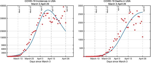
Table 3. Parameter estimation results: parameter estimates of the model (1(1) $\begin{array}{l}{\displaystyle S^{\prime }=-{\displaystyle \frac{{\beta }_{E}ES+{\beta }_n{I}_{n}S+{\beta }_s{I}_{s}S}{N-I_h}},}\\ {\displaystyle E^{\prime }={\displaystyle \frac{{\beta }_{E}ES+{\beta }_n{I}_{n}S+{\beta }_s{I}_{s}S}{N-I_h}}-kE,}\\ I_n^{\prime }=(1-\rho )kE-{\gamma }_n{I}_n,\\ I_s^{\prime }=\rho kE-(\alpha +{\gamma }_s)I_s,\\ I_h^{\prime }=\alpha I_s-({\gamma }_h+\nu )I_h,\\ R^{\prime }={\gamma }_n{I}_n+{\gamma }_s{I}_s+{\gamma }_h{I}_h.\end{array}$(1) ) obtained by solving the optimization problem (16(16) $\begin{array}{rl}\hat{\mathit{p}}& =\underset{\mathit{p}}{min}\left({\displaystyle \frac{1}{n}{\displaystyle \sum _{i=1}^n{\displaystyle \frac{|y_1(t_i)-Y_1^i{|}^2}{{\hat{Y}}_1^2}+{\displaystyle \frac{1}{m}{\displaystyle \sum _{j=1}^m{\displaystyle \frac{|y_2(t_j)-Y_2^j{|}^2}{{\hat{Y}}_2^2}}}}}}}\right)\text{w.r.t}\mathit{p}>0\\ & \text{and}{\beta }_s={\mathcal{R}}_0/\left({\displaystyle \frac{q_E}{k}+(1-\rho ){\displaystyle \frac{q_n}{{\gamma }_n}+\rho {\displaystyle \frac{1}{{\gamma }_s+\alpha }}}}\right){\displaystyle \frac{S(0)}{N(0)},\nu <1,1/28<{\gamma }_h<1/7,}\\ {\gamma }_s& <1,\alpha =0.1765{\gamma }_s\end{array}$(16) ).

Parameter	${\beta }_s$	$q_E$	$q_n$	α	${\gamma }_s$	${\gamma }_h$	ν
Estimated value	$6.6\times {10}^{-5}$	589.8	97394.6	0.006	0.03	$0.14$	0.86

3.3. Practical identifiability analysis

We continue the identifiability analysis by performing Monte Carlo Simulations (MCS) and study whether the parameters of the model can be estimated by solving the constraint minimization problem numerically (16(16) $\begin{array}{rl}\hat{\mathit{p}}& =\underset{\mathit{p}}{min}\left({\displaystyle \frac{1}{n}{\displaystyle \sum _{i=1}^n{\displaystyle \frac{|y_1(t_i)-Y_1^i{|}^2}{{\hat{Y}}_1^2}+{\displaystyle \frac{1}{m}{\displaystyle \sum _{j=1}^m{\displaystyle \frac{|y_2(t_j)-Y_2^j{|}^2}{{\hat{Y}}_2^2}}}}}}}\right)\text{w.r.t}\mathit{p}>0\\ & \text{and}{\beta }_s={\mathcal{R}}_0/\left({\displaystyle \frac{q_E}{k}+(1-\rho ){\displaystyle \frac{q_n}{{\gamma }_n}+\rho {\displaystyle \frac{1}{{\gamma }_s+\alpha }}}}\right){\displaystyle \frac{S(0)}{N(0)},\nu <1,1/28<{\gamma }_h<1/7,}\\ {\gamma }_s& <1,\alpha =0.1765{\gamma }_s\end{array}$(16) ) from the noisy observations $\mathit{Y}=(Y_1^i,Y_2^j)$ (15(15) $Y_1^i=y_1(t_i)+{ϵ}_{i}i=1,2,\dots ,n\text{and}{Y}_2^j=y_2(t_j)+{ϵ}_{j}j=1,2,\dots ,m$(15) ). This type of identifiability is called practical identifiability [22]. To determine the practical identifiability, first we estimate the model parameters by (16(16) $\begin{array}{rl}\hat{\mathit{p}}& =\underset{\mathit{p}}{min}\left({\displaystyle \frac{1}{n}{\displaystyle \sum _{i=1}^n{\displaystyle \frac{|y_1(t_i)-Y_1^i{|}^2}{{\hat{Y}}_1^2}+{\displaystyle \frac{1}{m}{\displaystyle \sum _{j=1}^m{\displaystyle \frac{|y_2(t_j)-Y_2^j{|}^2}{{\hat{Y}}_2^2}}}}}}}\right)\text{w.r.t}\mathit{p}>0\\ & \text{and}{\beta }_s={\mathcal{R}}_0/\left({\displaystyle \frac{q_E}{k}+(1-\rho ){\displaystyle \frac{q_n}{{\gamma }_n}+\rho {\displaystyle \frac{1}{{\gamma }_s+\alpha }}}}\right){\displaystyle \frac{S(0)}{N(0)},\nu <1,1/28<{\gamma }_h<1/7,}\\ {\gamma }_s& <1,\alpha =0.1765{\gamma }_s\end{array}$(16) ) using the reported daily incidences and deaths. Then using the estimated parameters $\hat{\mathit{p}}$, we generate synthetic data sets $\mathit{Y}=(Y_1^i,Y_2^j)$ which are contaminated with error. We perform the MCS with two different error structures: (i) normal distribution and (ii) Poisson distribution.

(i) Error structure with normal distribution: We assume that the measurement error is proportional to data. Namely we assume that the measurement error has the following form: ${ϵ}_i=y_1(t_i){\epsilon }_i\text{and similarly}{ϵ}_j=y_2(t_j){\epsilon }_j$where ${\epsilon }_i$ and ${\epsilon }_j$ are independent and identically distributed with mean zero and standard deviation ${\sigma }_0$. Thus the random variables $Y_1^i$ and $Y_2^j$ have mean $y_1(t_i)$ and $y_2(t_j)$ respectively, and standard deviation $y_1(t_i){\sigma }_0$ and $y_2(t_j){\sigma }_0$ respectively. In particular, we generate M = 1000 data sets using normal distribution whose mean is the model predictions and standard deviations are $y_1(t_i){\sigma }_0$ and $y_2(t_j){\sigma }_0$ respectively. That is (18) $Y_1^i=\mathcal{N}(y_1(t_i,\hat{\mathit{p}}),y_1(t_i,\hat{\mathit{p}}){\sigma }_0)\text{and}{Y}_2^j=\mathcal{N}(y_2(t_j,\hat{\mathit{p}}),y_2(t_j,\hat{\mathit{p}}){\sigma }_0)$(18) where $\mathcal{N}(\mu ,\sigma )$ denotes the normal distribution with mean μ and standard deviation σ.

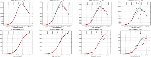
We generate M = 1000 synthetic data sets for each measurement errors, by increasing the errors gradually from ${\sigma }_0=1\mathrm{\%}$, to ${\sigma }_0=5\mathrm{\%},10\mathrm{\%}$ and ${\sigma }_0=20\mathrm{\%}$. In Figure 3, we present a single synthetic incidence ($Y_1^i$) and deaths ($Y_2^j$) for each measurement error ${\sigma }_0$. Comparing Figure 3 with the actual data in Figure 2, it appears the actual data has about $20\mathrm{\%}$ error.

Figure 3. Top row: A single set of incidences data generated for the Monte Carlo Simulations is presented for each measurement error. The incidence data is generated by taking the estimated parameters given in Table 3 as true parameters $\hat{\mathit{p}}$ and generating random incidences with normal distribution whose mean is $y_1(t_i,\hat{\mathit{p}})$ and the standard deviation is $y_1(t_i,\hat{\mathit{p}}){\sigma }_0$. Bottom row: The simulated deaths data is generated by taking the estimated parameters given in Table 3 and as true parameters $\hat{\mathit{p}}$ and generating random deaths with normal distribution whose mean is $y_2(t_i,\hat{\mathit{p}})$ and the standard deviation is $y_2(t_i,\hat{\mathit{p}}){\sigma }_0$ as in (18(18) $Y_1^i=\mathcal{N}(y_1(t_i,\hat{\mathit{p}}),y_1(t_i,\hat{\mathit{p}}){\sigma }_0)\text{and}{Y}_2^j=\mathcal{N}(y_2(t_j,\hat{\mathit{p}}),y_2(t_j,\hat{\mathit{p}}){\sigma }_0)$(18) ). First column is for ${\sigma }_0=1\mathrm{\%}$, the second column is for ${\sigma }_0=5\mathrm{\%}$, the second column is for ${\sigma }_0=10\mathrm{\%}$ and the fourth column is for ${\sigma }_0=20\mathrm{\%}$. We stopped at ${\sigma }_0=20\mathrm{\%}$, because comparison with the actual data suggests that the measurement error is about $20\mathrm{\%}$.

(ii) Error structure with poisson distribution: For the Poisson distribution, the mean and the standard deviation are equal. (19) $Y_1^i=\mathcal{P}(y_1(t_i,\hat{\mathit{p}}))\text{and}{Y}_2^j=\mathcal{P}(y_2(t_j,\hat{\mathit{p}}))$(19) where $\mathcal{P}(\mu )$ denotes the Poisson distribution with mean μ. We present the synthetic data generated by Poisson distribution in Figure 4. It is apparent from Figure 2, Figure 3 and Figure 4 that the error structure in actual data most likely has normal distribution with ${\sigma }_0=20\mathrm{\%}$.

Figure 4. Presents a single set of incidences and deaths data generated by Poisson error distribution. Data is generated by taking the estimated parameters given in Table 3 as true parameters $\hat{\mathit{p}}$ and generating random data with Poisson distribution.

We then fit the COVID-19 epidemic model (1(1) $\begin{array}{l}{\displaystyle S^{\prime }=-{\displaystyle \frac{{\beta }_{E}ES+{\beta }_n{I}_{n}S+{\beta }_s{I}_{s}S}{N-I_h}},}\\ {\displaystyle E^{\prime }={\displaystyle \frac{{\beta }_{E}ES+{\beta }_n{I}_{n}S+{\beta }_s{I}_{s}S}{N-I_h}}-kE,}\\ I_n^{\prime }=(1-\rho )kE-{\gamma }_n{I}_n,\\ I_s^{\prime }=\rho kE-(\alpha +{\gamma }_s)I_s,\\ I_h^{\prime }=\alpha I_s-({\gamma }_h+\nu )I_h,\\ R^{\prime }={\gamma }_n{I}_n+{\gamma }_s{I}_s+{\gamma }_h{I}_h.\end{array}$(1) ) to each M = 1000 data sets by solving the optimization problem (16(16) $\begin{array}{rl}\hat{\mathit{p}}& =\underset{\mathit{p}}{min}\left({\displaystyle \frac{1}{n}{\displaystyle \sum _{i=1}^n{\displaystyle \frac{|y_1(t_i)-Y_1^i{|}^2}{{\hat{Y}}_1^2}+{\displaystyle \frac{1}{m}{\displaystyle \sum _{j=1}^m{\displaystyle \frac{|y_2(t_j)-Y_2^j{|}^2}{{\hat{Y}}_2^2}}}}}}}\right)\text{w.r.t}\mathit{p}>0\\ & \text{and}{\beta }_s={\mathcal{R}}_0/\left({\displaystyle \frac{q_E}{k}+(1-\rho ){\displaystyle \frac{q_n}{{\gamma }_n}+\rho {\displaystyle \frac{1}{{\gamma }_s+\alpha }}}}\right){\displaystyle \frac{S(0)}{N(0)},\nu <1,1/28<{\gamma }_h<1/7,}\\ {\gamma }_s& <1,\alpha =0.1765{\gamma }_s\end{array}$(16) ) and then calculate the Average Relative Errors (AREs) of each parameter for each noise level. The AREs are computed as (20) $ARE(p^k)=100\mathrm{\%}{\displaystyle \frac{1}{M}{\displaystyle \sum _{j=1}^M{\displaystyle \frac{|{\hat{p}}^k-p_j^k|}{{\hat{p}}^k}}}}$(20) where $p^k$ is the $k^{th}$ parameter in $\mathit{p}$ and $\hat{\mathit{p}}$ are the parameters that generate the random variables $Y_1^i$ and $Y_2^j$. AREs of the parameters for each measurement error are presented in Table 4 and Table 5. AREs give insight about the practical identifiability of the model parameters. In Table 4, we present the AREs of each parameter when the error structure in the data is assumed to be normal. AREs of each parameter increases as the measurement error level (${\sigma }_0$) increases. We see that two of the parameters, namely ${\beta }_s$ and $q_E$ have high AREs compared to other parameters. The AREs of parameters ${\beta }_s$ and $q_E$ are more than the 20 times the measurement error when ${\sigma }_0=20\mathrm{\%}$. On the other hand, the AREs of the parameters $q_n,\nu ,{\gamma }_s$ and ${\gamma }_h$ are bounded by the measurement error at ${\sigma }_0=20\mathrm{\%}$. Based on AREs in Table 4, we conclude that the parameters ${\beta }_s$ and $q_E$ are not practically identifiable. Parameters $q_n,\nu ,{\gamma }_s$ and ${\gamma }_h$ are practically identifiable.

Table 4. Monte Carlo simulation results: Average relative errors (ARE)s of parameters of the COVID-19 model (1(1) $\begin{array}{l}{\displaystyle S^{\prime }=-{\displaystyle \frac{{\beta }_{E}ES+{\beta }_n{I}_{n}S+{\beta }_s{I}_{s}S}{N-I_h}},}\\ {\displaystyle E^{\prime }={\displaystyle \frac{{\beta }_{E}ES+{\beta }_n{I}_{n}S+{\beta }_s{I}_{s}S}{N-I_h}}-kE,}\\ I_n^{\prime }=(1-\rho )kE-{\gamma }_n{I}_n,\\ I_s^{\prime }=\rho kE-(\alpha +{\gamma }_s)I_s,\\ I_h^{\prime }=\alpha I_s-({\gamma }_h+\nu )I_h,\\ R^{\prime }={\gamma }_n{I}_n+{\gamma }_s{I}_s+{\gamma }_h{I}_h.\end{array}$(1) ) are presented after performing parameter estimation problem (16(16) $\begin{array}{rl}\hat{\mathit{p}}& =\underset{\mathit{p}}{min}\left({\displaystyle \frac{1}{n}{\displaystyle \sum _{i=1}^n{\displaystyle \frac{|y_1(t_i)-Y_1^i{|}^2}{{\hat{Y}}_1^2}+{\displaystyle \frac{1}{m}{\displaystyle \sum _{j=1}^m{\displaystyle \frac{|y_2(t_j)-Y_2^j{|}^2}{{\hat{Y}}_2^2}}}}}}}\right)\text{w.r.t}\mathit{p}>0\\ & \text{and}{\beta }_s={\mathcal{R}}_0/\left({\displaystyle \frac{q_E}{k}+(1-\rho ){\displaystyle \frac{q_n}{{\gamma }_n}+\rho {\displaystyle \frac{1}{{\gamma }_s+\alpha }}}}\right){\displaystyle \frac{S(0)}{N(0)},\nu <1,1/28<{\gamma }_h<1/7,}\\ {\gamma }_s& <1,\alpha =0.1765{\gamma }_s\end{array}$(16) ) to M = 1000 synthetic data sets for each measurement error ${\sigma }_0$.

	${\sigma }_0=1\mathrm{\%}$	${\sigma }_0=5\mathrm{\%}$	${\sigma }_0=10\mathrm{\%}$	${\sigma }_0=20\mathrm{\%}$
Parameter	ARE	ARE	ARE	ARE
${\beta }_s$	78	238	294	426
$q_E$	13.7	41.2	77.7	628.6
$q_n$	9.1	11.9	14.3	18.1
ν	2.6	4.9	6.1	7.9
${\gamma }_s$	1.3	3.4	4.6	7.6
${\gamma }_h$	3.7	11.8	14.4	17.5

Table 5. Monte Carlo simulation results: average relative errors (ARE)s and $95\mathrm{\%}$ confidence intervals of parameters of the COVID-19 model (1(1) $\begin{array}{l}{\displaystyle S^{\prime }=-{\displaystyle \frac{{\beta }_{E}ES+{\beta }_n{I}_{n}S+{\beta }_s{I}_{s}S}{N-I_h}},}\\ {\displaystyle E^{\prime }={\displaystyle \frac{{\beta }_{E}ES+{\beta }_n{I}_{n}S+{\beta }_s{I}_{s}S}{N-I_h}}-kE,}\\ I_n^{\prime }=(1-\rho )kE-{\gamma }_n{I}_n,\\ I_s^{\prime }=\rho kE-(\alpha +{\gamma }_s)I_s,\\ I_h^{\prime }=\alpha I_s-({\gamma }_h+\nu )I_h,\\ R^{\prime }={\gamma }_n{I}_n+{\gamma }_s{I}_s+{\gamma }_h{I}_h.\end{array}$(1) ) are presented after performing parameter estimation problem (16(16) $\begin{array}{rl}\hat{\mathit{p}}& =\underset{\mathit{p}}{min}\left({\displaystyle \frac{1}{n}{\displaystyle \sum _{i=1}^n{\displaystyle \frac{|y_1(t_i)-Y_1^i{|}^2}{{\hat{Y}}_1^2}+{\displaystyle \frac{1}{m}{\displaystyle \sum _{j=1}^m{\displaystyle \frac{|y_2(t_j)-Y_2^j{|}^2}{{\hat{Y}}_2^2}}}}}}}\right)\text{w.r.t}\mathit{p}>0\\ & \text{and}{\beta }_s={\mathcal{R}}_0/\left({\displaystyle \frac{q_E}{k}+(1-\rho ){\displaystyle \frac{q_n}{{\gamma }_n}+\rho {\displaystyle \frac{1}{{\gamma }_s+\alpha }}}}\right){\displaystyle \frac{S(0)}{N(0)},\nu <1,1/28<{\gamma }_h<1/7,}\\ {\gamma }_s& <1,\alpha =0.1765{\gamma }_s\end{array}$(16) ) to M = 1000 synthetic data sets with Poisson error structure.

Parameter	ARE	Confidence Interval
${\beta }_s$	49	$[6.4\times {10}^{-4},3.0\times {10}^{-4}]$
$q_E$	10.7	$[142,674]$
$q_n$	8.2	$[21673,99999]$
ν	3.3	$[0.825,0.953]$
${\gamma }_s$	2.2	$[0.0298,0.0334]$
${\gamma }_h$	7.4	$[0.0845,0.1429]$

Next we run the MCS by generating M = 1000 data sets using Poisson error structure with mean $y_1(t_i,\hat{\mathit{p}})$ and $y_2(t_i,\hat{\mathit{p}})$. We then compute the AREs and the results are presented in Table 5. Checking the ARE of each parameter in Table 5, we see that the parameters ${\beta }_s$ and $q_E$ have higher ARE compared to other parameters and declare these parameters to be practically unidentifiable. Comparing the ARE values in Table 4 with ARE values in Table 5, regardless of the error structure assumption, Normal vs. Poisson, we see that in both cases the parameters ${\beta }_s$ and $q_E$ have significantly higher AREs compared to other parameters. In conclusion, error structure does not influence the parameter identifiability.

We continue with the identifiability analysis by assessing the evolution of the parameter identifiability. Thus we investigate how the parameter identifiability changes as function of time. We performed the MCS simulations at three different stages of the pandemic; (i) before it reached its peak, (ii) at the peak and (iii) after the peak. Since normal error structure is a better representation of the error structure in the actual data, we performed the MC simulations with normal error structure. We present the AREs of each parameter before the peak and at the peak in Table 6. AREs presented in Table 4 are the AREs of the parameters after the peak. The AREs of the infection rate of symptomatic individuals, (${\beta }_s$) decrease as the pandemic progresses, same is true for $q_n$. We do not observe the decline of the AREs for the parameter $q_E$. On the other hand, AREs of the parameters ν and ${\gamma }_s$ remain almost the same for all three phases of the pandemic. And AREs of the parameter ${\gamma }_s$ increase from before the peak to at the peak phase and then decrease again from the peak to the after the peak phase. For this practical identifiability analysis, we conclude that as the pandemic progresses, as we add more data points to the parameter estimation problem, it is not possible to say that the identifiability of the parameters improves.

Table 6. Monte Carlo simulation results: Average relative errors (ARE)s of parameters of the COVID-19 model (1(1) $\begin{array}{l}{\displaystyle S^{\prime }=-{\displaystyle \frac{{\beta }_{E}ES+{\beta }_n{I}_{n}S+{\beta }_s{I}_{s}S}{N-I_h}},}\\ {\displaystyle E^{\prime }={\displaystyle \frac{{\beta }_{E}ES+{\beta }_n{I}_{n}S+{\beta }_s{I}_{s}S}{N-I_h}}-kE,}\\ I_n^{\prime }=(1-\rho )kE-{\gamma }_n{I}_n,\\ I_s^{\prime }=\rho kE-(\alpha +{\gamma }_s)I_s,\\ I_h^{\prime }=\alpha I_s-({\gamma }_h+\nu )I_h,\\ R^{\prime }={\gamma }_n{I}_n+{\gamma }_s{I}_s+{\gamma }_h{I}_h.\end{array}$(1) ) are presented after performing parameter estimation problem (16(16) $\begin{array}{rl}\hat{\mathit{p}}& =\underset{\mathit{p}}{min}\left({\displaystyle \frac{1}{n}{\displaystyle \sum _{i=1}^n{\displaystyle \frac{|y_1(t_i)-Y_1^i{|}^2}{{\hat{Y}}_1^2}+{\displaystyle \frac{1}{m}{\displaystyle \sum _{j=1}^m{\displaystyle \frac{|y_2(t_j)-Y_2^j{|}^2}{{\hat{Y}}_2^2}}}}}}}\right)\text{w.r.t}\mathit{p}>0\\ & \text{and}{\beta }_s={\mathcal{R}}_0/\left({\displaystyle \frac{q_E}{k}+(1-\rho ){\displaystyle \frac{q_n}{{\gamma }_n}+\rho {\displaystyle \frac{1}{{\gamma }_s+\alpha }}}}\right){\displaystyle \frac{S(0)}{N(0)},\nu <1,1/28<{\gamma }_h<1/7,}\\ {\gamma }_s& <1,\alpha =0.1765{\gamma }_s\end{array}$(16) ) to M = 1000 synthetic data sets for each measurement error ${\sigma }_0$. Error structure is assumed to be normal.

Before the peak					At the peak
	${\sigma }_0=1\mathrm{\%}$	${\sigma }_0=5\mathrm{\%}$	${\sigma }_0=10\mathrm{\%}$	${\sigma }_0=20\mathrm{\%}$	Parameter	${\sigma }_0=1\mathrm{\%}$	${\sigma }_0=5\mathrm{\%}$	${\sigma }_0=10\mathrm{\%}$	${\sigma }_0=20\mathrm{\%}$
Parameter	ARE	ARE	ARE	ARE		ARE	ARE	ARE	ARE
${\beta }_s$	106	512	1023	2520	${\beta }_s$	21	179	270	1359
$q_E$	24.5	52.2	74.1	126.2	$q_E$	10.5	33.9	120.1	267
$q_n$	19.5	24.6	23.4	25.7	$q_n$	8.5	14.1	17.4	24.9
ν	2.2	4.9	6.1	7.8	ν	2	4	6	9.6
${\gamma }_s$	1.7	3.7	5.6	13.1	${\gamma }_s$	2.4	4.9	7.7	15.6
${\gamma }_h$	8.4	14.3	16.7	17.3	${\gamma }_h$	51.2	98.9	115.7	123.3

4. Forecasting multiple outbreak waves and determining control strategies

4.1. Predicting the future epidemic waves

Kermack–McKendrick type SEIR epidemic model (M₁(M$_1$) $\mathbf{M}\mathbf{o}\mathbf{d}\mathbf{e}\mathbf{l}\mathbf{1}\mathbf{(}{\mathbf{M}}_{\mathbf{1}}\mathbf{)}\mathbf{:}\{\begin{array}{l}{\displaystyle S^{\prime }=-\frac{{\beta }_{E}ES+\beta IS}{N},}\\ {\displaystyle E^{\prime }=\frac{{\beta }_{E}ES+\beta IS}{N}-kE,}\\ I^{\prime }=kE-(\nu +\gamma )I,\\ R^{\prime }=\gamma I.\end{array}$(M$_1$) ) or its variations such as (M₂(M$_2$) $\mathbf{M}\mathbf{o}\mathbf{d}\mathbf{e}\mathbf{l}\mathbf{2}\mathbf{(}{\mathbf{M}}_{\mathbf{2}}\mathbf{)}\mathbf{:}\{\begin{array}{l}{\displaystyle S^{\prime }=-\frac{{\beta }_{E}ES+{\beta }_n{I}_{n}S+{\beta }_s{I}_{s}S}{N},}\\ {\displaystyle E^{\prime }=\frac{{\beta }_{E}ES+{\beta }_n{I}_{n}S+{\beta }_s{I}_{s}S}{N}-kE,}\\ I_n^{\prime }=(1-\rho )kE-{\gamma }_n{I}_n,\\ I_s^{\prime }=\rho kE-(\nu +{\gamma }_s)I_s,\\ R^{\prime }={\gamma }_n{I}_n+{\gamma }_s{I}_s.\end{array}$(M$_2$) ) and (1(1) $\begin{array}{l}{\displaystyle S^{\prime }=-{\displaystyle \frac{{\beta }_{E}ES+{\beta }_n{I}_{n}S+{\beta }_s{I}_{s}S}{N-I_h}},}\\ {\displaystyle E^{\prime }={\displaystyle \frac{{\beta }_{E}ES+{\beta }_n{I}_{n}S+{\beta }_s{I}_{s}S}{N-I_h}}-kE,}\\ I_n^{\prime }=(1-\rho )kE-{\gamma }_n{I}_n,\\ I_s^{\prime }=\rho kE-(\alpha +{\gamma }_s)I_s,\\ I_h^{\prime }=\alpha I_s-({\gamma }_h+\nu )I_h,\\ R^{\prime }={\gamma }_n{I}_n+{\gamma }_s{I}_s+{\gamma }_h{I}_h.\end{array}$(1) ) can only forecast a single outbreak wave. Due to their nature, these types of outbreak models cannot predict multiple epidemic waves. In this section, we give a methodology on how to use an epidemic model to predict multiple waves. We use the methodology used in sub-epidemic curves introduced in [6]. Authors in [6] used a single generalized-logistic growth model which describes the incidences to forecast multiple epidemic waves. Here we generalize this methodology to outbreak models. We model the epidemic wave which consist of three overlapping sub-epidemics using the COVID-19 model (1(1) $\begin{array}{l}{\displaystyle S^{\prime }=-{\displaystyle \frac{{\beta }_{E}ES+{\beta }_n{I}_{n}S+{\beta }_s{I}_{s}S}{N-I_h}},}\\ {\displaystyle E^{\prime }={\displaystyle \frac{{\beta }_{E}ES+{\beta }_n{I}_{n}S+{\beta }_s{I}_{s}S}{N-I_h}}-kE,}\\ I_n^{\prime }=(1-\rho )kE-{\gamma }_n{I}_n,\\ I_s^{\prime }=\rho kE-(\alpha +{\gamma }_s)I_s,\\ I_h^{\prime }=\alpha I_s-({\gamma }_h+\nu )I_h,\\ R^{\prime }={\gamma }_n{I}_n+{\gamma }_s{I}_s+{\gamma }_h{I}_h.\end{array}$(1) ): (21) $\begin{array}{l}{\displaystyle S_i^{\prime }=-A_i(t)\left(\frac{{\beta }_{E_i}{E}_i{S}_i+{\beta }_{n_i}{I}_{n_i}{S}_i+{\beta }_{s_i}{I}_{s_i}{S}_i}{N_i-I_{h_i}}\right),}\\ {\displaystyle E_i^{\prime }=A_i(t)(\frac{{\beta }_{E_i}{E}_i{S}_i+{\beta }_{n_i}{I}_{n_i}{S}_i+{\beta }_{s_i}{I}_{s_i}{S}_i}{N_i-I_{h_i}}-k_i{E}_i),}\\ I_{n_i}^{\prime }=A_i(t)((1-{\rho }_i)k_i{E}_i-{\gamma }_{n_i}{I}_{n_i}),\\ I_{s_i}^{\prime }=A_i(t)({\rho }_i{k}_i{E}_i-({\alpha }_i+{\gamma }_{s_i})I_{s_i}),\\ I_{h_i}^{\prime }=A_i(t)({\alpha }_i{I}_{s_i}-({\gamma }_{h_i}+{\nu }_i)I_{h_i}),\\ R_i^{\prime }=A_i(t)({\gamma }_{n_i}{I}_{n_i}+{\gamma }_{s_i}{I}_{s_i}+{\gamma }_{h_i}{I}_{h_i}),\end{array}$(21) where $A_i(t)=\{\begin{array}{cc}0& \mathrm{for}t<t_i\\ 1& \mathrm{for}t\ge t_i\end{array}$for i = 1, 2, 3 with $t_1<t_2<t_3$ and $t_1=0$. For the sub-epidemic model (21(21) $\begin{array}{l}{\displaystyle S_i^{\prime }=-A_i(t)\left(\frac{{\beta }_{E_i}{E}_i{S}_i+{\beta }_{n_i}{I}_{n_i}{S}_i+{\beta }_{s_i}{I}_{s_i}{S}_i}{N_i-I_{h_i}}\right),}\\ {\displaystyle E_i^{\prime }=A_i(t)(\frac{{\beta }_{E_i}{E}_i{S}_i+{\beta }_{n_i}{I}_{n_i}{S}_i+{\beta }_{s_i}{I}_{s_i}{S}_i}{N_i-I_{h_i}}-k_i{E}_i),}\\ I_{n_i}^{\prime }=A_i(t)((1-{\rho }_i)k_i{E}_i-{\gamma }_{n_i}{I}_{n_i}),\\ I_{s_i}^{\prime }=A_i(t)({\rho }_i{k}_i{E}_i-({\alpha }_i+{\gamma }_{s_i})I_{s_i}),\\ I_{h_i}^{\prime }=A_i(t)({\alpha }_i{I}_{s_i}-({\gamma }_{h_i}+{\nu }_i)I_{h_i}),\\ R_i^{\prime }=A_i(t)({\gamma }_{n_i}{I}_{n_i}+{\gamma }_{s_i}{I}_{s_i}+{\gamma }_{h_i}{I}_{h_i}),\end{array}$(21) ), the observation of incidences and deaths becomes respectively as follows: $y_1(t)={\rho }_1{k}_1{E}_1+{\rho }_2{k}_2{E}_2+{\rho }_3{k}_3{E}_3\mathrm{and}{y}_2(t)={\nu }_1{I}_{h_1}+{\nu }_2{I}_{h_2}+{\nu }_3{I}_{h_3}.$To estimate the model parameters, we modified the optimization problem (16(16) $\begin{array}{rl}\hat{\mathit{p}}& =\underset{\mathit{p}}{min}\left({\displaystyle \frac{1}{n}{\displaystyle \sum _{i=1}^n{\displaystyle \frac{|y_1(t_i)-Y_1^i{|}^2}{{\hat{Y}}_1^2}+{\displaystyle \frac{1}{m}{\displaystyle \sum _{j=1}^m{\displaystyle \frac{|y_2(t_j)-Y_2^j{|}^2}{{\hat{Y}}_2^2}}}}}}}\right)\text{w.r.t}\mathit{p}>0\\ & \text{and}{\beta }_s={\mathcal{R}}_0/\left({\displaystyle \frac{q_E}{k}+(1-\rho ){\displaystyle \frac{q_n}{{\gamma }_n}+\rho {\displaystyle \frac{1}{{\gamma }_s+\alpha }}}}\right){\displaystyle \frac{S(0)}{N(0)},\nu <1,1/28<{\gamma }_h<1/7,}\\ {\gamma }_s& <1,\alpha =0.1765{\gamma }_s\end{array}$(16) ) for the sub-epidemic model (21(21) $\begin{array}{l}{\displaystyle S_i^{\prime }=-A_i(t)\left(\frac{{\beta }_{E_i}{E}_i{S}_i+{\beta }_{n_i}{I}_{n_i}{S}_i+{\beta }_{s_i}{I}_{s_i}{S}_i}{N_i-I_{h_i}}\right),}\\ {\displaystyle E_i^{\prime }=A_i(t)(\frac{{\beta }_{E_i}{E}_i{S}_i+{\beta }_{n_i}{I}_{n_i}{S}_i+{\beta }_{s_i}{I}_{s_i}{S}_i}{N_i-I_{h_i}}-k_i{E}_i),}\\ I_{n_i}^{\prime }=A_i(t)((1-{\rho }_i)k_i{E}_i-{\gamma }_{n_i}{I}_{n_i}),\\ I_{s_i}^{\prime }=A_i(t)({\rho }_i{k}_i{E}_i-({\alpha }_i+{\gamma }_{s_i})I_{s_i}),\\ I_{h_i}^{\prime }=A_i(t)({\alpha }_i{I}_{s_i}-({\gamma }_{h_i}+{\nu }_i)I_{h_i}),\\ R_i^{\prime }=A_i(t)({\gamma }_{n_i}{I}_{n_i}+{\gamma }_{s_i}{I}_{s_i}+{\gamma }_{h_i}{I}_{h_i}),\end{array}$(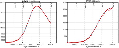21) ). The estimated parameters are presented in Table 7. The fit is shown in Figure 5.

Figure 5. Blue curve is the prediction of the sub-epidemic model (21(21) $\begin{array}{l}{\displaystyle S_i^{\prime }=-A_i(t)\left(\frac{{\beta }_{E_i}{E}_i{S}_i+{\beta }_{n_i}{I}_{n_i}{S}_i+{\beta }_{s_i}{I}_{s_i}{S}_i}{N_i-I_{h_i}}\right),}\\ {\displaystyle E_i^{\prime }=A_i(t)(\frac{{\beta }_{E_i}{E}_i{S}_i+{\beta }_{n_i}{I}_{n_i}{S}_i+{\beta }_{s_i}{I}_{s_i}{S}_i}{N_i-I_{h_i}}-k_i{E}_i),}\\ I_{n_i}^{\prime }=A_i(t)((1-{\rho }_i)k_i{E}_i-{\gamma }_{n_i}{I}_{n_i}),\\ I_{s_i}^{\prime }=A_i(t)({\rho }_i{k}_i{E}_i-({\alpha }_i+{\gamma }_{s_i})I_{s_i}),\\ I_{h_i}^{\prime }=A_i(t)({\alpha }_i{I}_{s_i}-({\gamma }_{h_i}+{\nu }_i)I_{h_i}),\\ R_i^{\prime }=A_i(t)({\gamma }_{n_i}{I}_{n_i}+{\gamma }_{s_i}{I}_{s_i}+{\gamma }_{h_i}{I}_{h_i}),\end{array}$(21) ) to US COVID-19 cases and deaths (bars).

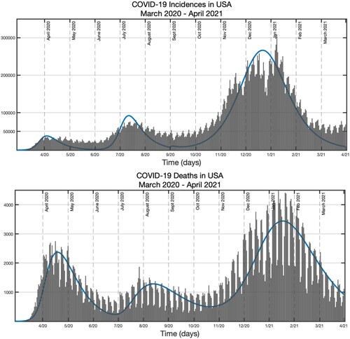
Table 7. Parameter estimation results: parameter estimates of the sub-epidemic model (21(21) $\begin{array}{l}{\displaystyle S_i^{\prime }=-A_i(t)\left(\frac{{\beta }_{E_i}{E}_i{S}_i+{\beta }_{n_i}{I}_{n_i}{S}_i+{\beta }_{s_i}{I}_{s_i}{S}_i}{N_i-I_{h_i}}\right),}\\ {\displaystyle E_i^{\prime }=A_i(t)(\frac{{\beta }_{E_i}{E}_i{S}_i+{\beta }_{n_i}{I}_{n_i}{S}_i+{\beta }_{s_i}{I}_{s_i}{S}_i}{N_i-I_{h_i}}-k_i{E}_i),}\\ I_{n_i}^{\prime }=A_i(t)((1-{\rho }_i)k_i{E}_i-{\gamma }_{n_i}{I}_{n_i}),\\ I_{s_i}^{\prime }=A_i(t)({\rho }_i{k}_i{E}_i-({\alpha }_i+{\gamma }_{s_i})I_{s_i}),\\ I_{h_i}^{\prime }=A_i(t)({\alpha }_i{I}_{s_i}-({\gamma }_{h_i}+{\nu }_i)I_{h_i}),\\ R_i^{\prime }=A_i(t)({\gamma }_{n_i}{I}_{n_i}+{\gamma }_{s_i}{I}_{s_i}+{\gamma }_{h_i}{I}_{h_i}),\end{array}$(21) ).

Parameter	${\beta }_{s_1}$	$q_{E_1}$	$q_{n_1}$	${\gamma }_{s_1}$	${\gamma }_{h_1}$	${\nu }_1$
Estimated value	$4.2\times {10}^{-5}$	5428	47368	0.05	$0.14$	0.24

4.2. An optimal control scenario

US states initiated various community mitigation policies in March 2020. Some of the widely implemented strategies included the issuance of orders requiring persons to stay home, schools were closed and universities transitioned to online instruction. Stay-at-home orders started from California on March 19, 2020, and ultimately were issued in all 50 states, covering 316 million people between March 19 and May 20, 2020 [30]. To model the social distancing, we introduce control $u_1(t)$ which effectively reduces the transmission rates for the exposed E and non-symptomatic individuals $I_n$. To model the self-isolation required from symptomatic individuals $I_s$, we introduce a control $u_2(t)$. Although, direct correspondence between the real life controls, social distancing and self-isolation to our controls $u_1$ and $u_2$ is not clear, such an investigation still yields to useful observations, particularly in the extreme case, when we want to achieve maximum effect. Both controls belong to the admissible set $\mathcal{A}=\{u\in {\mathit{L}}^1(0,T)|0\le u(t)\le 1\}$where T is the final time considered. The model with the controls takes the following form: (22) $\begin{array}{l}{\displaystyle S^{\prime }=-{\beta }_s{\displaystyle \frac{q_E(1-u_1)ES+q_n(1-u_1)I_{n}S+(1-u_2)I_{s}S}{N-I_h}}}\\ {\displaystyle E^{\prime }={\beta }_s{\displaystyle \frac{q_E(1-u_1)ES+q_n(1-u_1)I_{n}S+(1-u_2)I_{s}S}{N-I_h}}-kE}\\ I_n^{\prime }=(1-\rho )kE-{\gamma }_n{I}_n\\ I_s^{\prime }=\rho I_s-(\alpha +{\gamma }_s)I_s\\ I_h^{\prime }=\alpha I_s-({\gamma }_h+\nu )I_h\\ R^{\prime }=\gamma I_n+{\gamma }_s{I}_s+{\gamma }_h{I}_h\end{array}$(22) The main goal of the quarantine was to reduce the total number of infected individuals over the time $[0,T]$. To express that we use the following cost functional: (23) $\mathcal{J}(u_1,u_2)={\int }_0^T(E+I_n+I_s+I_h+B_1{u}_1^2+B_2{u}_2^2)\mathrm{d}t={\int }_0^{T}L(\mathit{x},u)\mathrm{d}t$(23) Our goal is to find an optimal control functions $(u_1^{\ast },u_2^{\ast })$ such that $J(u_1^{\ast },u_2^{\ast })={\displaystyle \underset{u\in \mathcal{A}}{min}J(u_1,u_2)\mathrm{subjected}\mathrm{to}\mathrm{the}\mathrm{system}(20)}$We do not consider isolation to be a control variable, as isolation was applied only to severe cases. Since 80–85% are mild to moderate [23], hospitalizations are determined by the progression to severe symptoms and cannot be controlled.

We use Pontryagin's Minimum Principle [20] and introduce a time-varying Lagrange multiplier vector $\lambda (t)$, whose elements are called the adjoint variables of the system. The Hamiltonian $\mathcal{H}$ is defined $\mathrm{\forall }t\in [0,T]$ by (24) $\mathcal{H}(\mathit{x},u,\lambda )=L(\mathit{x},u)+\sum _{i=1}^6{\lambda }_i{f}_i(\mathit{x},u)$(24) That is we set Hamiltonian as (25) $\begin{array}{rl}\mathcal{H}(\mathit{x},u,\lambda )& =E+I_n+I_s+I_h+B_1{u}_1^2+B_2{u}_2^2\\ & +{\lambda }_1(-{\beta }_s{\displaystyle \frac{q_E(1-u_1)ES+q_n(1-u_1)I_{n}S+(1-u_2)I_{s}S}{N-I_h}})\\ & +{\lambda }_2\left({\beta }_s{\displaystyle \frac{q_E(1-u_1)ES+q_n(1-u_1)I_{n}S+(1-u_2)I_{s}S}{N-I_h}-kE}\right)\\ & +{\lambda }_3((1-\rho )kE-{\gamma }_n{I}_n)\\ & +{\lambda }_4(\rho kE-(\alpha +{\gamma }_s)I_s)\\ & +{\lambda }_5(\alpha I_s-({\gamma }_h+\nu )I_h)\\ & +{\lambda }_6({\gamma }_n{I}_n+{\gamma }_s{I}_s+{\gamma }_h{I}_h).\end{array}$(25) In the next theorem, we present the adjoint system and optimal control characterizations.

Theorem 4.1

Given an optimal pair $(x^{\ast },u^{\ast })$, there exists adjoint variables ${\lambda }_i$, $i=1,2,\dots ,6$ such that $\begin{array}{rl}{\displaystyle {\lambda }_1^{\prime }}& =({\lambda }_1-{\lambda }_2)\frac{{\beta }_E(1-u_1)E+{\beta }_n(1-u_1)I_n+{\beta }_s(1-u_2)I_s}{S+E+I_n+I_s+R}\\ & +({\lambda }_2-{\lambda }_1)\frac{{\beta }_E(1-u_1)ES+{\beta }_n(1-u_1)I_{n}S+{\beta }_s(1-u_2)I_{s}S}{(S+E+I_n+I_s+R{)}^2}\\ {\displaystyle {\lambda }_2^{\prime }}& =-1+({\lambda }_1-{\lambda }_2)\frac{{\beta }_E(1-u_1)S}{S+E+I_n+I_s+R}+({\lambda }_2-{\lambda }_1)\\ & \times \frac{{\beta }_E(1-u_1)ES+{\beta }_n(1-u_1)I_{n}S+{\beta }_s(1-u_2)I_{s}S}{(S+E+I_n+I_s+R{)}^2}\\ & +({\lambda }_2-{\lambda }_3)k+({\lambda }_3-{\lambda }_4)\rho k\\ {\displaystyle {\lambda }_3^{\prime }}& =-1+({\lambda }_1-{\lambda }_2)\frac{{\beta }_n(1-u_1)S}{(S+E+I_n+I_s+R)}+({\lambda }_2-{\lambda }_1)\\ & \times \frac{{\beta }_E(1-u_1)ES+{\beta }_n(1-u_1)I_{n}S+{\beta }_s(1-u_2)I_{s}S}{(S+E+I_n+I_s+R{)}^2}\\ & +({\lambda }_3-{\lambda }_6){\gamma }_n\\ {\displaystyle {\lambda }_4^{\prime }}& =-1+({\lambda }_1-{\lambda }_2)\frac{{\beta }_s(1-u_2)S}{S+E+I_n+I_s+R}+({\lambda }_2-{\lambda }_1)\\ & \times \frac{{\beta }_E(1-u_1)ES+{\beta }_n(1-u_1)I_{n}S+{\beta }_s(1-u_2)I_{s}S}{(S+E+I_n+I_s+R{)}^2}\\ & +({\lambda }_4-{\lambda }_5)\alpha +({\lambda }_4-{\lambda }_6){\gamma }_s\\ {\displaystyle {\lambda }_5^{\prime }}& =-1+({\lambda }_5-{\lambda }_6)r+{\lambda }_5\nu \\ {\displaystyle {\lambda }_6^{\prime }}& =({\lambda }_2-{\lambda }_1)\frac{{\beta }_E(1-u_1)ES+{\beta }_n(1-u_1)I_{n}S+{\beta }_s(1-u_2)I_{s}S}{(S+E+I_n+I_s+R{)}^2}\end{array}$with ${\lambda }_i(T)=0$ for $i=1,2,\dots ,6$. The optimal controls $u^{\ast }=(u_1^{\ast },u_2^{\ast })$ are represented by (26) $\begin{array}{r}{\displaystyle u_1^{\ast }=min(1,max(0,\frac{({\lambda }_2-{\lambda }_1)S({\beta }_{E}E+{\beta }_n{I}_n)}{2B_1(S+E+I_n+I_s+R)}))}\end{array}$(26) (27) $\begin{array}{r}{\displaystyle u_2^{\ast }=min(1,max(0,\frac{({\lambda }_2-{\lambda }_1){\beta }_s{I}_{s}S}{2B_2(S+E+I_n+I_s+R)}))}\end{array}$(27)

Proof.

Pontryagin minimum principle states that for the optimality of control $u^{\ast }(t)$ and corresponding trajectory ${\mathit{x}}^{\ast }$ with $\mathrm{\forall }t\in [0,T]$, it is necessary that there exist a nonzero adjoint vector function ${\lambda }^{\ast }(t)$ which is a solution to the adjoint system (28) $\{\begin{array}{l}{\lambda }^{\prime }(t)={\displaystyle -{\displaystyle \frac{\mathrm{\partial }\mathcal{H}(\mathit{x},u,\lambda )}{\mathrm{\partial }\mathit{x}}}}\\ \lambda (T)=0\end{array}$(28) Setting ${\lambda }_1^{\prime }=-{\displaystyle \frac{\mathrm{\partial }H}{\mathrm{\partial }S},{\lambda }_2^{\prime }=-{\displaystyle \frac{\mathrm{\partial }H}{\mathrm{\partial }E},{\lambda }_3^{\prime }=-{\displaystyle \frac{\mathrm{\partial }H}{\mathrm{\partial }{I}_n},{\lambda }_4^{\prime }=-{\displaystyle \frac{\mathrm{\partial }H}{\mathrm{\partial }{I}_s},{\lambda }_5^{\prime }=-{\displaystyle \frac{\mathrm{\partial }H}{\mathrm{\partial }{I}_h},{\lambda }_6^{\prime }=-{\displaystyle \frac{\mathrm{\partial }H}{\mathrm{\partial }R}}}}}}}$we obtain the adjoint system with $\lambda (T)=0$. By the optimality condition, ${\displaystyle \frac{\mathrm{\partial }\mathcal{H}}{\mathrm{\partial }{u}_1}=2B_1{u}_1+\frac{{\lambda }_1{\beta }_{E}ES+{\lambda }_1{\beta }_n{I}_{n}S}{(N-I_h)}-\frac{{\lambda }_2{\beta }_{E}ES+{\lambda }_2{\beta }_n{I}_{n}S}{(N-I_h)}=0}$we obtain ${\displaystyle u_1^{\ast }=\frac{({\lambda }_2-{\lambda }_1)S({\beta }_{E}E+{\beta }_n{I}_n)}{2B_1(S+E+I_n+I_s+R)}}$Similarly, ${\displaystyle \frac{\mathrm{\partial }\mathcal{H}}{\mathrm{\partial }{u}_2}=2B_2{u}_2+\frac{{\lambda }_1{\beta }_s{I}_{s}S-{\lambda }_2{\beta }_s{I}_{s}S}{N-I_h}=0⟹{\displaystyle u_2^{\ast }=\frac{({\lambda }_2-{\lambda }_1){\beta }_s{I}_{s}S}{2B_2(S+E+I_n+I_s+R)}}}$Notice that $\frac{{\mathrm{\partial }}^2\mathcal{H}}{\mathrm{\partial }{u}_1^2}=2B_1\ge 0$, and $\frac{{\mathrm{\partial }}^2\mathcal{H}}{\mathrm{\partial }{u}_2^2}=2B_2\ge 0.$ Since, $u^{\ast }\in \mathcal{A}$ we set $\begin{array}{rl}{\displaystyle u_1^{\ast }}& =min(1,max(0,\frac{({\lambda }_2-{\lambda }_1)S({\beta }_{E}E+{\beta }_n{I}_n)}{2B_1(S+E+I_n+I_s+R)}))\mathrm{and}\\ u_2^{\ast }& =min(1,max(0,\frac{({\lambda }_2-{\lambda }_1){\beta }_s{I}_{s}S}{2B_2(S+E+I_n+I_s+R)}))\end{array}$

4.2.1. Numerical simulations with optimal control

We use forward–backward sweep method [18] to approximate the solution of model (22(22) $\begin{array}{l}{\displaystyle S^{\prime }=-{\beta }_s{\displaystyle \frac{q_E(1-u_1)ES+q_n(1-u_1)I_{n}S+(1-u_2)I_{s}S}{N-I_h}}}\\ {\displaystyle E^{\prime }={\beta }_s{\displaystyle \frac{q_E(1-u_1)ES+q_n(1-u_1)I_{n}S+(1-u_2)I_{s}S}{N-I_h}}-kE}\\ I_n^{\prime }=(1-\rho )kE-{\gamma }_n{I}_n\\ I_s^{\prime }=\rho I_s-(\alpha +{\gamma }_s)I_s\\ I_h^{\prime }=\alpha I_s-({\gamma }_h+\nu )I_h\\ R^{\prime }=\gamma I_n+{\gamma }_s{I}_s+{\gamma }_h{I}_h\end{array}$(22) ) with controls $u_1,u_2$. We use MATLAB built-in function ode15s to approximate the solutions of the model (22(22) $\begin{array}{l}{\displaystyle S^{\prime }=-{\beta }_s{\displaystyle \frac{q_E(1-u_1)ES+q_n(1-u_1)I_{n}S+(1-u_2)I_{s}S}{N-I_h}}}\\ {\displaystyle E^{\prime }={\beta }_s{\displaystyle \frac{q_E(1-u_1)ES+q_n(1-u_1)I_{n}S+(1-u_2)I_{s}S}{N-I_h}}-kE}\\ I_n^{\prime }=(1-\rho )kE-{\gamma }_n{I}_n\\ I_s^{\prime }=\rho I_s-(\alpha +{\gamma }_s)I_s\\ I_h^{\prime }=\alpha I_s-({\gamma }_h+\nu )I_h\\ R^{\prime }=\gamma I_n+{\gamma }_s{I}_s+{\gamma }_h{I}_h\end{array}$(22) ) with controls by taking initial conditions $\mathit{x}(0)={\mathit{x}}_0$ and also use the ode15s to solve the adjoint differential differential equations backward in time by taking the value at the final time as $\lambda (T)=0$. We use the following forward–backward sweep algorithm to get the optimal control functions [18].

1. Take initial guesses for $u=(u_1(t),u_2(t))$

2. Solve for the state function differential Equation (22(22) $\begin{array}{l}{\displaystyle S^{\prime }=-{\beta }_s{\displaystyle \frac{q_E(1-u_1)ES+q_n(1-u_1)I_{n}S+(1-u_2)I_{s}S}{N-I_h}}}\\ {\displaystyle E^{\prime }={\beta }_s{\displaystyle \frac{q_E(1-u_1)ES+q_n(1-u_1)I_{n}S+(1-u_2)I_{s}S}{N-I_h}}-kE}\\ I_n^{\prime }=(1-\rho )kE-{\gamma }_n{I}_n\\ I_s^{\prime }=\rho I_s-(\alpha +{\gamma }_s)I_s\\ I_h^{\prime }=\alpha I_s-({\gamma }_h+\nu )I_h\\ R^{\prime }=\gamma I_n+{\gamma }_s{I}_s+{\gamma }_h{I}_h\end{array}$(22) ) using ode15s forward in time.

3. Solve for the adjoint function differential Equation ${\lambda }_i^{\prime }(t)=\frac{\mathrm{\partial }\mathcal{H}}{\mathrm{\partial }{\mathit{x}}_i},\lambda (T)=0$ using ode15s backward in time.

4. We update the new values of $u=(u_1(t),u_2(t))$ using (26(26) $\begin{array}{r}{\displaystyle u_1^{\ast }=min(1,max(0,\frac{({\lambda }_2-{\lambda }_1)S({\beta }_{E}E+{\beta }_n{I}_n)}{2B_1(S+E+I_n+I_s+R)}))}\end{array}$(26) ) and(27(27) $\begin{array}{r}{\displaystyle u_2^{\ast }=min(1,max(0,\frac{({\lambda }_2-{\lambda }_1){\beta }_s{I}_{s}S}{2B_2(S+E+I_n+I_s+R)}))}\end{array}$(27) ).

5. Iterate the same process until the following convergence criteria is met for every state variable, adjoint and control functions ${\displaystyle \frac{\Vert x^k-x^{k-1}\Vert }{\Vert x^k\Vert }<\delta \mathrm{and}{\displaystyle \frac{\Vert u^k-u^{k-1}\Vert }{\Vert u^k\Vert }<\delta \mathrm{and}{\displaystyle \frac{\Vert {\lambda }^k-{\lambda }^{k-1}\Vert }{\Vert {\lambda }^k\Vert }<\delta \mathrm{for}\delta >0.}}}$

For the optimal control simulations, we use the parameter values obtained in the fitting as presented in Table 3. For the first simulation, we solve the optimal control problem with controls social distancing and self-isolation setting off at time t = 0 and effective for 75 days. Figure 6 presents the state of infectious populations with and without social distancing and self-isolation. We see that the controls are most effective when it is applied at $100\mathrm{\%}$, that is at their upper bound of 1. We recognize that achieving 100% social distancing or isolation is not practically possible. However our results show that the higher the social distancing or isolation the lower the infection. Therefore, depending on the level of the cost parameters and our cost structure, one should aim at the maximum possible social distancing and isolation. Even if we set a realistic upper bound, $u_{max}$ for the controls which is strictly less than 1, the optimal control will still reside at the $u_{max}$ most of the time. For the next simulation, we apply the social distancing and self-isolation from March 19 till May 20, for about 2 months as this was the case for the USA. We perform the iterative process to find the optimal pair which would be only effective from March 19 till May 20 that would minimize the objective function (23(23) $\mathcal{J}(u_1,u_2)={\int }_0^T(E+I_n+I_s+I_h+B_1{u}_1^2+B_2{u}_2^2)\mathrm{d}t={\int }_0^{T}L(\mathit{x},u)\mathrm{d}t$(23) ) subject to the COVID-19 model (22(22) $\begin{array}{l}{\displaystyle S^{\prime }=-{\beta }_s{\displaystyle \frac{q_E(1-u_1)ES+q_n(1-u_1)I_{n}S+(1-u_2)I_{s}S}{N-I_h}}}\\ {\displaystyle E^{\prime }={\beta }_s{\displaystyle \frac{q_E(1-u_1)ES+q_n(1-u_1)I_{n}S+(1-u_2)I_{s}S}{N-I_h}}-kE}\\ I_n^{\prime }=(1-\rho )kE-{\gamma }_n{I}_n\\ I_s^{\prime }=\rho I_s-(\alpha +{\gamma }_s)I_s\\ I_h^{\prime }=\alpha I_s-({\gamma }_h+\nu )I_h\\ R^{\prime }=\gamma I_n+{\gamma }_s{I}_s+{\gamma }_h{I}_h\end{array}$(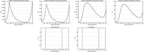22) ) starting on March 3 and ending on June 23, 2020. In Figure 7, we only present the infectious states with controls, since the infectious populations without controls are same as in Figure 6 second row. Comparing Figure 6 and Figure 7, we see that, one of the main differences in starting the social distancing and self-isolation 2 weeks after the launch of the outbreak is that the number of infectious classes are at least 1 magnitude order higher if not more. Further, we see, comparing Figure 6 with Figure 7 that if we had continue to apply the controls there would not have been an uptick in cases.

Figure 6. Simulations of the COVID-19 model with control measures (22(22) $\begin{array}{l}{\displaystyle S^{\prime }=-{\beta }_s{\displaystyle \frac{q_E(1-u_1)ES+q_n(1-u_1)I_{n}S+(1-u_2)I_{s}S}{N-I_h}}}\\ {\displaystyle E^{\prime }={\beta }_s{\displaystyle \frac{q_E(1-u_1)ES+q_n(1-u_1)I_{n}S+(1-u_2)I_{s}S}{N-I_h}}-kE}\\ I_n^{\prime }=(1-\rho )kE-{\gamma }_n{I}_n\\ I_s^{\prime }=\rho I_s-(\alpha +{\gamma }_s)I_s\\ I_h^{\prime }=\alpha I_s-({\gamma }_h+\nu )I_h\\ R^{\prime }=\gamma I_n+{\gamma }_s{I}_s+{\gamma }_h{I}_h\end{array}$(22) ). First row: Infectious populations with control. Seconfd row: Infectious populations without control. Third row: Self-isolation and social distancing controls. The weights in the objective functional are $B_1=B_2=1$.

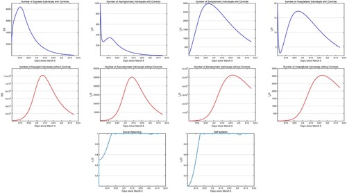
Figure 7. Simulations of the COVID-19 model with control measures (22(22) $\begin{array}{l}{\displaystyle S^{\prime }=-{\beta }_s{\displaystyle \frac{q_E(1-u_1)ES+q_n(1-u_1)I_{n}S+(1-u_2)I_{s}S}{N-I_h}}}\\ {\displaystyle E^{\prime }={\beta }_s{\displaystyle \frac{q_E(1-u_1)ES+q_n(1-u_1)I_{n}S+(1-u_2)I_{s}S}{N-I_h}}-kE}\\ I_n^{\prime }=(1-\rho )kE-{\gamma }_n{I}_n\\ I_s^{\prime }=\rho I_s-(\alpha +{\gamma }_s)I_s\\ I_h^{\prime }=\alpha I_s-({\gamma }_h+\nu )I_h\\ R^{\prime }=\gamma I_n+{\gamma }_s{I}_s+{\gamma }_h{I}_h\end{array}$(22) ). First row: Infectious populations with control. Second row: Self-isolation and social distancing controls. Controls start on March 19 and end on May 20, last for 60 days. The weights in the objective functional are $B_1=B_2=1$.

5. Discussion

Mathematical compartmental models can provide valuable insight about the spread of SARS-CoV-2 in a population. In particular, they can provide guidance about the role of specific interventions in reducing the impact of an ongoing disease outbreak. All models are limited by factors that include the levels of complexity in the epidemiological states being considered, the parameters to be estimated, and the limited data that often involves delay and uncertainty. These models have the potential to provide valuable guidance for pandemic preparedness and planning to reduce the burden of an outbreak, particularly during the early phase of an outbreak. In this study, we proposed a COVID-19 epidemic model that considers six epidemic states and incorporates important phases of the coronavirus life cycle, such as incubation and latency period. Scenarios that incorporate social distancing efforts are implemented to limit the spread of SARS-CoV-2 were considered in our study. We computed the reproduction number, estimated model parameters based on daily cases and deaths, and conducted structural and practical identifiability analysis for the proposed model.

We show that parameters of the proposed model are not structurally identifiable from observations of daily incidence and deaths. We further establish that for a sequence of models, nested in the proposed model, only the SEIR model where all incidences are observed, is structurally identifiable. For our proposed model, we show that if the parameters α, ${\gamma }_n$, k, ρ are fixed from external information, then all parameters are structurally identifiable, except ${\beta }_s$. To identify ${\beta }_s$ we use estimates of ${\mathcal{R}}_0$ from the literature.

We further investigated the practical identifiability of these parameters by performing Monte Carlo Simulations and found that transmission rate for exposed ${\beta }_E=q_E{\beta }_s$ and symptomatic infectious ${\beta }_s$ were not practically identifiable. This result largely persists even if we use outside information for the proportion of individuals who progress to hospitalization. A surprising outcome of the practical identifiability analysis was that fixing the proportion of individuals who become hospitalized in fact makes the parameters of the model practically identifiable. The practical identifiability conclusions remain the same regardless of the error structure (Poisson or Normal) chosen. We also investigated whether taking a shorter time series compared to taking a longer time series affected identifiability results. For the most part identifiability improved with the longer data set but we think that the results were not strong enough and uniform enough to be conclusive.

The investigation of the optimal control problem shows that socials distancing should be practiced at 100% to reduce the disease quickly, while isolation can be practiced at more relaxed conditions, particularly as time progresses. Social distancing should be practiced at 100% for most of the time interval even if the cost of that is very high. High levels of social distancing lead to exceptionally high reduction in the number infected individuals without symptoms and hospitalized individuals which leads to quick curtailing of the pandemic and maintenance of susceptible individuals at higher level.

An important finding of our study is our investigation of social distancing and self-isolation as control measures. We investigated two scenarios: control is active during the entire studied interval of time and the control is active only when the lock down was in effect, which is a subset of time. With the first scenario both optimal controls gradually go to the maximum and stay there for the remainder of the studied duration. In this case, the epidemic states are well controlled and reach peaks at least an order of magnitude smaller than with the second scenario when the control is applied with delay. In the second scenario, the optimal controls jump to the maximum and stay there for the entire allowed duration. However, the numbers in the infected classes are much larger, and as soon as the control is stopped, these classes start growing in magnitude. The observation we make here support again the rule of thumb that control measures have to be applied as early as possible in an epidemic as strongly as possible. Our numerical simulations for each of the epidemic states of the proposed model show the critical importance of the timely implementation of control measures, particularly in reducing the number of individuals at risk of exposure and infection from the coronavirus. The implications of these findings are most relevant during the very early phase of the pandemic as the simulations are based on data captured very early-on. To further investigate the trajectories of these epidemic states and parameters as the pandemic progresses beyond its early phase, we fit overlapping epidemic waves to the data of the USA as described by [6]. This allows us to investigate how the virus and epidemic characteristics of the COVID-19 pandemic have evolved over the year since it first became established in the USA. To accurately model the spread of the coronavirus and the role of specific interventions, it is important that we update modelling efforts to account for new virus information, as well as additional relevant interventions such as testing and contact tracing [3,12,17]. It is also important to consider that morbidity and mortality associated with COVID-19 differ among individuals in the population and such trends in risk have also evolved over time [7,24,37]. During the early phase of the COVID-19 pandemic in the USA older age individuals seemed to have experienced a higher burden while in the current months of this pandemic, younger and mid-age individuals seem to experience higher risk of infection. A consistent observation with this pandemic is that individuals of older age, and higher pre-existing comorbidities such as heart disease, diabetes and obesity have a higher risk of infection and severe COVID-19 experience [15,25,28].

In summary, this study presents a COVID-19 model that investigates the spread of SARS-CoV-2 and the role control interventions play to reduce the burden associated with the COVID-19 pandemic. In particular, our study of the structural and practical identifiability of the proposed model highlights the importance of parameter identifiability and the limitations inherent to uncertainty in data available, particularly during the early phase of a novel pandemic. We have presented some unique methodology for turning unidentifiable into identifiable parameters. Using a mixed approach to the problem of parameter identifiability, we are able to provide specific guidance about the identifiability of a subset of parameters that can be useful in guiding some of the model predictions. We further investigate the relevance of control measures through social distancing efforts and self-isolation. We show that the timely implementation of control measures can be extremely valuable to reduce the burden of this novel pandemic.

We present all Matlab code for parameter estimation and Monte Carlo Simulations at https://github.com/NecibeTuncer/Idenitifiability_COVID-19_Early_in_Pandemic together with the DAISY and Mathematica results for the identifiability analysis.

Disclosure statement

No potential conflict of interest was reported by the author(s).

Appendix

A.1. SEIR model

Input–output equations for the SEIR model (M₁(M$_1$) $\mathbf{M}\mathbf{o}\mathbf{d}\mathbf{e}\mathbf{l}\mathbf{1}\mathbf{(}{\mathbf{M}}_{\mathbf{1}}\mathbf{)}\mathbf{:}\{\begin{array}{l}{\displaystyle S^{\prime }=-\frac{{\beta }_{E}ES+\beta IS}{N},}\\ {\displaystyle E^{\prime }=\frac{{\beta }_{E}ES+\beta IS}{N}-kE,}\\ I^{\prime }=kE-(\nu +\gamma )I,\\ R^{\prime }=\gamma I.\end{array}$(M$_1$) ), where $y_1(t)=kE,y_2(t)=\nu I.$ (A1) $\begin{array}{rl}0& =\frac{\mathrm{d}{y}_2}{\mathrm{d}t}-y_1\nu +y_2(\nu +\alpha )\\ 0& =\frac{{\mathrm{d}}^3{y}_1}{\mathrm{d}{t}^3}\frac{\mathrm{d}{y}_1}{\mathrm{d}t}{y}_1^2{\beta }^2{\nu }^2+\frac{d^3{y}_1}{d{t}^3}\frac{\mathrm{d}{y}_1}{\mathrm{d}t}{y}_1{y}_2\beta \nu k(2{\beta }_E-\nu )+\frac{d^3{y}_1}{d{t}^3}\frac{\mathrm{d}{y}_1}{\mathrm{d}t}{y}_2^2{\beta }_E{k}^2({\beta }_E-\nu )+\frac{d^3{y}_1}{d{t}^3}{y}_1^3{\beta }^2{\nu }^{2}k\\ & +\frac{d^3{y}_1}{d{t}^3}{y}_1^2{y}_2\beta \nu k^2(2{\beta }_E-\nu )+\frac{d^3{y}_1}{d{t}^3}{y}_1{y}_2^2{\beta }_E{k}^3({\beta }_E-\nu )-{\frac{{\mathrm{d}}^2{y}_1}{\mathrm{d}{t}^2}}^2{y}_1^2{\beta }^2{\nu }^2\\ & +2{\frac{{\mathrm{d}}^2{y}_1}{\mathrm{d}{t}^2}}^2{y}_1{y}_2\beta \nu k(-{\beta }_E+\nu )\\ & +{\frac{{\mathrm{d}}^2{y}_1}{\mathrm{d}{t}^2}}^2{y}_2^2{\beta }_E{k}^2(-{\beta }_E+2\nu )-2\frac{{\mathrm{d}}^2{y}_1}{\mathrm{d}{t}^2}{\frac{\mathrm{d}{y}_1}{\mathrm{d}t}}^2{y}_1{\beta }^2{\nu }^2+\frac{{\mathrm{d}}^2{y}_1}{\mathrm{d}{t}^2}{\frac{\mathrm{d}{y}_1}{\mathrm{d}t}}^2{y}_2\beta \nu k(-2{\beta }_E-\nu )\\ & +\frac{{\mathrm{d}}^2{y}_1}{\mathrm{d}{t}^2}\frac{\mathrm{d}{y}_1}{\mathrm{d}t}{y}_1^2\beta {\nu }^{2}k(-4\beta -{\beta }_E+\nu )\\ & +\frac{{\mathrm{d}}^2{y}_1}{\mathrm{d}{t}^2}\frac{\mathrm{d}{y}_1}{\mathrm{d}t}{y}_1{y}_2\nu k(\beta {\beta }_E\nu +\beta {\beta }_E\alpha -5\beta {\beta }_{E}k-\beta {\nu }^2-\beta \nu \alpha +3\beta \nu k-{\beta }_E^{2}k-{\beta }_E\nu k)\\ & +\frac{{\mathrm{d}}^2{y}_1}{\mathrm{d}{t}^2}\frac{\mathrm{d}{y}_1}{\mathrm{d}t}{y}_2^2{\beta }_E{k}^2({\beta }_E\nu +{\beta }_E\alpha -{\beta }_{E}k+{\nu }^2+\nu \alpha +3\nu k)+\frac{{\mathrm{d}}^2{y}_1}{\mathrm{d}{t}^2}{y}_1^3\beta {\nu }^2{k}^2(-{\beta }_E+\nu )\\ & +\frac{{\mathrm{d}}^2{y}_1}{\mathrm{d}{t}^2}{y}_1^2{y}_2\nu k^2(\beta {\beta }_E\nu +\beta {\beta }_E\alpha +\beta {\beta }_{E}k-\beta {\nu }^2-\beta \nu \alpha -{\beta }_E^{2}k-{\beta }_E\nu k)\\ & +\frac{{\mathrm{d}}^2{y}_1}{\mathrm{d}{t}^2}{y}_1{y}_2^2{\beta }_E{k}^3({\beta }_E\nu +{\beta }_E\alpha +{\beta }_{E}k+{\nu }^2+\nu \alpha -\nu k)+2{\frac{\mathrm{d}{y}_1}{\mathrm{d}t}}^4{\beta }^2{\nu }^2\\ & +{\frac{\mathrm{d}{y}_1}{\mathrm{d}t}}^3{y}_1\beta {\nu }^{2}k(3\beta +3{\beta }_E-\nu )\\ & +{\frac{\mathrm{d}{y}_1}{\mathrm{d}t}}^3{y}_2\nu k(-4\beta {\beta }_E\nu -4\beta {\beta }_E\alpha -\beta {\beta }_{E}k+\beta {\nu }^2+\beta \nu \alpha -2\beta \nu k-{\beta }_E^{2}k+{\beta }_E\nu k)\\ & +{\frac{\mathrm{d}{y}_1}{\mathrm{d}t}}^2{y}_1^2{d}^{2}k(\beta {\beta }_E\nu +\beta {\beta }_E\alpha +5\beta {\beta }_{E}k-\beta \nu k+2{\beta }_E^{2}k-{\beta }_E\nu k)\\ & +{\frac{\mathrm{d}{y}_1}{\mathrm{d}t}}^2{y}_1{y}_2\nu k(-\beta {\beta }_E{\nu }^2-2\beta {\beta }_E\nu \alpha -7\beta {\beta }_E\nu k-\beta {\beta }_E{\alpha }^2-7\beta {\beta }_E\alpha k-3\beta {\beta }_E{k}^2\\ & +\beta {\nu }^{2}k+\beta \nu \alpha k-3{\beta }_E^2\nu k-3{\beta }_E^2\alpha k-3{\beta }_E^2{k}^2+{\beta }_E{\nu }^{2}k+{\beta }_E\nu \alpha k+{\beta }_E\nu k^2)\\ & +{\frac{\mathrm{d}{y}_1}{\mathrm{d}t}}^2{y}_2^2{\beta }_E{k}^2({\beta }_E{\nu }^2+2{\beta }_E\nu \alpha +{\beta }_E\nu k+{\beta }_E{\alpha }^2+{\beta }_E\alpha k-{\beta }_E{k}^2+{\nu }^{2}k+\nu \alpha k+2\nu k^2)\\ & +2\frac{\mathrm{d}{y}_1}{\mathrm{d}t}{y}_1^3{\beta }_E{\nu }^2{k}^2(\beta \nu +\beta \alpha +\beta k+2{\beta }_{E}k-\nu k)+\frac{\mathrm{d}{y}_1}{\mathrm{d}t}{y}_1^2{y}_2{\beta }_E\nu k^2\\ & \times (-2\beta {\nu }^2-4\beta \nu \alpha -3\beta \nu k-2\beta {\alpha }^2-3\beta \alpha k-6{\beta }_E\nu k-6{\beta }_E\alpha k-2{\beta }_E{k}^2+2{\nu }^{2}k+2\nu \alpha k)\\ & +\frac{\mathrm{d}{y}_1}{\mathrm{d}t}{y}_1{y}_2^2{\beta }_E{k}^3(2{\beta }_E{\nu }^2+4{\beta }_E\nu \alpha +{\beta }_E\nu k+2{\beta }_E{\alpha }^2+{\beta }_E\alpha k+{\nu }^{2}k+\nu \alpha k)\\ & +y_1^4{\beta }_E{\nu }^2{k}^3(\beta \nu +\beta \alpha +2{\beta }_{E}k-\nu k)+y_1^3{y}_2{\beta }_E\nu k^3(-\beta {\nu }^2-2\beta \nu \alpha \\ & -\beta {\alpha }^2-3{\beta }_E\nu k-3{\beta }_E\alpha k+{\nu }^{2}k+\nu \alpha k)+y_1^2{y}_2^2{\beta }_E^2{k}^4({\nu }^2+2\nu \alpha +{\alpha }^2)\end{array}$(A1)

References

- G. Bellu, M.P. Saccomani, S. Audoly, and L. D'Angio, Daisy – differential algebra for identifiability of systems, Available at https://daisy.dei.unipd.it.
- H.R. Bhapkar, P.N. Mahalle, N. Dey, and K.C. Santosh, Revisited covid-19 mortality and recovery rates: Are we missing recovery time period?, J. Med. Syst. 44 (2020), pp. 1–5.
- A. Bilinski, F. Mostashari, and J.A. Salomon, Modeling contact tracing strategies for covid-19 in the context of relaxed physical distancing measures, JAMA network open 3(8) (2020), pp. e2019217.
- CDC, Severe outcomes among patients with coronavirus disease 2019 (covid-19) –united states, february 12–march 16, 2020, MMWR 69 (2020), pp. 343–346.
- K. Roosa and G. Chowell, Assessing parameter identifiability in compartmental dynamic models using a computational approach: application to infectious disease transmission models, Theoretical Biol. Med. Model. 16 (2019), pp. 1–15.
- G. Chowell, A. Tariq, and J.M. Hyman, A novel sub-epidemic modeling framework for short-term forecasting epidemic waves, BMC. Med. 17 (2019), pp. 1–18.
- R.M. Colombo, M. Garavello, F. Marcellini, and E. Rossi, An age and space structured sir model describing the covid-19 pandemic, medRxiv 10 (2020), pp. 1–20.
- R. Dandekar and G. Barbastathis, Quantifying the effect of quarantine control in covid-19 infectious spread using machine learning, medRxiv2020
- M.C. Eisenberg and Y-H. Kao, Practical unidentifiability of a simple vector-borne disease model: Implications for parameter estimation and intervention assessment, Epidemics 25 (2018), pp. 89–100.
- M.C. Eisenberg, S.L. Robertson, and J.H. Tien, Identifiability and estimation of multiple transmission pathways in cholera and waterborne disease, J. Theor. Biol. 324 (2013), pp. 84–102.
- C. Elias, A. Sekri, P. Leblanc, M. Cucherat, and P. Vanhems, The incubation period of covid-19: A meta-analysis, Int. J. Infect. Dis. 104 (2021), pp. 708–710.
- G. Giordano, F. Blanchini, R. Bruno, P. Colaneri, A. Di Filippo, A. Di Matteo, and M. Colaneri, Modelling the covid-19 epidemic and implementation of population-wide interventions in italy, Nat. Med. 26 (2020), pp. 855–860.
- G. González-Parra and A.J. Arenas, Qualitative analysis of a mathematical model with presymptomatic individuals and two sars-cov-2 variants, Computational and Applied Mathematics 40 (2021), pp. 1–25.
- X. He, E. Lau, P. Wu, X. Deng, J. Wang, X. Hao, Y.C. Lau, J. Wong, Y. Guan, X. Tan, X. Mo, Y. Chen, B. Liao, W. Chen, F. Hu, Q. Zhang, M. Zhong, Y. Wu, L. Zhao, F. Zhang, B. Cowling, F. Li, and G. Leung, Temporal dynamics in viral shedding and transmissibility of covid-19, Nat. Med. 26 (2020), pp. 672–675.
- C. Huang, Y. Wang, X. Li, L. Ren, J. Zhao, Y. Hu, L. Zhang, G. Fan, J. Xu, X. Gu, and Z. Cheng, Clinical features of patients infected with 2019 novel coronavirus in wuhan, china, The lancet 395(10223) (2020), pp. 497–506.
- G.G. Katul, A. Mrad, S. Bonetti, G. Manoli, and A.J. Parolari, Global convergence of covid-19 basic reproduction number and estimation from early-time sir dynamics, PLoS. ONE. 15 (2020), pp. e023980.
- A.J. Kucharski, P. Klepac, A. Conlan, S.M. Kissler, M. Tang, H. Fry, J. Gog, and J. Edmunds, CMMID COVID-19 Working Group: et al. Effectiveness of isolation, testing, contact tracing and physical distancing on reducing transmission of sars-cov-2 in different settings, medRxiv 20 (2020), pp. 1151–1160.
- S. Lenhart and J.T. Workman, Optimal control applied to biological models, CRC press, 2007.
- F.S. Lu, A.T. Nguyen, N.B. Link, J.T. Davis, M. Chinazzi, X. Xiong, A. Vespignani, M. Lipsitch, and M. Santillana, Estimating the cumulative incidence of covid-19 in the united states using four complementary approaches, medRxiv2020
- M. Martcheva, An introduction to mathematical epidemiology, Springer, Vol. 61, 2015.
- G. Massonis, J.R. Banga, and A.F. Villaverde, Structural identifiability and observability of compartmental models of the covid-19 pandemic, Annu. Rev. Control. 51 (2020), pp. 441–459.
- H. Miao, X. Xia, A.S. Perelson, and H. Wu, On identifiability of nonlinear ode models and applications in viral dynamics, SIAM. Rev. Soc. Ind. Appl. Math. 53 (2011), pp. 3–39.
- N.J.M. Michelen and C. Stavropoulou, In patients of covid-19, what are the symptoms and clinical features of mild and moderate cases? - cebm, preprint (2020 Apr). Available at http://www.cebm.net/covid-19/in-patients-of-covid-19-what-are-the-symptoms-and-clinical-features-of-mild-and-moderate-case/, [cited 31 Oct 2020].
- R. Omori, R. Matsuyama, and Y. Nakata, The age distribution of mortality from novel coronavirus disease (covid-19) suggests no large difference of susceptibility by age, Sci. Rep. 10(1) (2020), pp. 1–9.
- G. Onder, G. Rezza, and S. Brusaferro, Case-fatality rate and characteristics of patients dying in relation to covid-19 in italy, Jama 323(18) (2020), pp. 1775–1776.
- J.M. Read, J.R.E. Bridgen, D.A.T. Cummings, A. Ho, and C.P. Jewell, Novel coronavirus 2019-ncov: early estimation of epidemiological parameters and epidemic predictions, MedRxiv. 2020.
- A. Sakurai, T. Sasaki, and S. Kato, et al Natural history of asymptomatic sars-cov-2 infection, N. Engl. J. Med. 383 (2020), pp. 885–886.
- Y-J. Sun, Y-J. Feng, J. Chen, B. Li, Z.-C. Luo, and P.-X. Wang, Clinical features of fatalities in patients with covid-19, Disaster. Med. Public. Health. Prep. 15 (2020), pp. e9–11.
- B. Tang, X. Wang, Q. Li, N.L. Bragazzi, S. Tang, Y. Xiao, and J. Wu, Estimation of the transmission risk of the 2019-ncov and its implication for public health interventions, J. Clin. Med. 9(2) (2020), pp. 462.
- The New York Times, See which states and cities have told residents to stay at home - the new york times, Available at https://www.nytimes.com/interactive/2020/us/coronavirus-stay-at-home-order.html. [cited 31 Oct 2020].
- C. Tsay, F. Lejarza, M.A. Stadtherr, and M. Baldea, Modeling, state estimation, and optimal control for the us covid-19 outbreak, preprint (2020). Available at arXiv:2004.06291.
- N. Tuncer, H. Gulbudak, V. Cannataro, and M. Martcheva, Structural and practical identifiability issues of immuno-epidemiological vector-host models with application to rift valley fever, Bull. Math. Biol. 78 (2016), pp. 1796–1827.
- N. Tuncer, B. Labarre, S. Payoute, and M. Martcheva, Structural and practical identifiability analysis of zika epidemiological models, Bull. Math. Biol. 80 (2018), pp. 2209–2241.
- N. Tuncer and T. Le, Structural and practical identifiability analysis of outbreak models, Math. Biosci. 299 (2018), pp. 1–18.
- N. Tuncer, C. Mohanakumar, S. Swanson, and M. Martcheva, Efficacy of control measures in the control of ebola, liberia 2014–2015, J. Biol. Dyn. 12(1) (2018), pp. 913–937.
- United states coronavirus, 9, 332, 958 cases and 235, 420 deaths - worldometer, preprint (2020 Oct). Available at https://www.worldometers.info/coronavirus/country/us/, [cited 31 Oct 2020].
- B. Wilder, M. Charpignon, J.A. Killian, H.-C. Ou, A. Mate, S. Jabbari, A. Perrault, A.N. Desai, M. Tambe, and M.S. Majumder, Modeling between-population variation in covid-19 dynamics in hubei, lombardy, and new york city, Proceedings of the National Academy of Sciences 117(41) (2020), pp. 25904–25910.
- J.T. Wu, K. Leung, and G.M. Leung, Nowcasting and forecasting the potential domestic and international spread of the 2019-ncov outbreak originating in wuhan, china: a modelling study, The Lancet 395(10225) (2020), pp. 689–697.
- S.L. Wu, A.N. Mertens, A. Crider, S. Yoshika, N.N.N. Pokpongkiat, S. Djajadi, A. Seth, M.S. Hsiang, J.M. Colford, A. Reingold, B.F. Arnold, A. Hubbard, and J. Benjamin-Chung, Substantial underestimation of sars-cov-2 infection in the united states, Nat. Commun. 11 (2020), pp. 1–10.
- Z. Yang, Z. Zeng, K. Wang, S-S. Wong, W. Liang, M. Zanin, P. Liu, X. Cao, Z. Gao, and Z. Mai, et al Modified seir and ai prediction of the epidemics trend of covid-19 in china under public health interventions, J. Thorac. Dis. 12(3) (2020), pp. 165.
- D. Zou, L. Wang, P. Xu, J. Chen, W. Zhang, and Q. Gu, Epidemic model guided machine learning for covid-19 forecasts in the united states, medRxiv, 2020.
Appendix
A.1. SEIR model
Input–output equations for the SEIR model (EquationM1(M$_1$)