Full article: Estimation of spreading speeds and travelling waves for the lattice pioneer-climax competition system

Formulae display: $MathJax Logo$ ?Mathematical formulae have been encoded as MathML and are displayed in this HTML version using MathJax in order to improve their display. Uncheck the box to turn MathJax off. This feature requires Javascript. Click on a formula to zoom.

ABSTRACT

This paper concerns the invasion dynamics of the lattice pioneer-climax competition model with parameter regions in which the system is non-monotone. We estimate the spreading speeds and establish appropriate conditions under which the spreading speeds are linearly selected. Moreover, the existence of travelling waves is determined by constructing suitable upper and lower solutions. It shows that the spreading speed coincides with the minimum wave speed of travelling waves if the diffusion rate of the invasive species is larger or equal to that of the native species. Our results are new to estimate the spreading speed of non-monotone lattice pioneer-climax systems, and the techniques developed in this work can be used to study the invasion dynamics of the pioneer-climax system with interaction delays, which could extend the results in the literature. The analysis replies on the construction of auxiliary systems, upper and lower solutions, and the monotone dynamical system approach.

KEYWORDS:

2020 MATHEMATICS SUBJECT CLASSIFICATIONS:

1. Introduction

In this work, we study the invasion dynamics of the following lattice pioneer-climax competition system arising from spatial population ecology: (1) ${\begin{aligned} \frac{d u_{j}}{d t} = d_{1} D_{2} [u_{j}] (t) + u_{j} (t) f (c_{11} u_{j} (t) + c_{12} v_{j} (t)) - h_{1} u_{j} (t), \\ \frac{d v_{j}}{d t} = d_{2} D_{2} [v_{j}] (t) + v_{j} (t) g (c_{21} u_{j} (t) + c_{22} v_{j} (t)) - h_{2} v_{j} (t), t \in R^{+}, j \in Z, \end{aligned}$ (1) where $D_{2} [u_{j}] (t) = u_{j + 1} (t) + u_{j - 1} (t) - 2 u_{j} (t)$ , $D_{2} [v_{j}] (t) = v_{j + 1} (t) + v_{j - 1} (t) - 2 v_{j} (t)$ . The model (Equation1(1) ${\begin{aligned} \frac{d u_{j}}{d t} = d_{1} D_{2} [u_{j}] (t) + u_{j} (t) f (c_{11} u_{j} (t) + c_{12} v_{j} (t)) - h_{1} u_{j} (t), \\ \frac{d v_{j}}{d t} = d_{2} D_{2} [v_{j}] (t) + v_{j} (t) g (c_{21} u_{j} (t) + c_{22} v_{j} (t)) - h_{2} v_{j} (t), t \in R^{+}, j \in Z, \end{aligned}$ (1) ) describes the diffusion and interaction between a pioneer species and a climax species, which are located on the patches of a one-dimensional lattice. The variables $u_{j} (t)$ and $v_{j} (t)$ represent the population densities of two species at patch j and time t, respectively. It is assumed that the spatial diffusion of two species only occurs among the nearest neighbours, and the positive constants $d_{1}$ and $d_{2}$ are diffusion coefficients. The species' per capita growth rates f and g in model (Equation1(1) ${\begin{aligned} \frac{d u_{j}}{d t} = d_{1} D_{2} [u_{j}] (t) + u_{j} (t) f (c_{11} u_{j} (t) + c_{12} v_{j} (t)) - h_{1} u_{j} (t), \\ \frac{d v_{j}}{d t} = d_{2} D_{2} [v_{j}] (t) + v_{j} (t) g (c_{21} u_{j} (t) + c_{22} v_{j} (t)) - h_{2} v_{j} (t), t \in R^{+}, j \in Z, \end{aligned}$ (1) ) depend on the linear combination of population densities of both pioneer and climax species weighted by the inter- and intra-specific competitive effects. Taking species 1 to be the pioneer species and species 2 to be the climax species, then the constant $c_{mn} > 0, m, n = 1, 2$ denotes the competitive effect of species n on species m. The linear terms $h_{1} u_{j}$ and $h_{2} v_{j}$ represent the constant effort harvesting [Citation1,Citation2] with $h_{i} > 0$ , or stocking with $h_{i} < 0, i = 1, 2.$ For example, for a forest ecosystem, the forest manager may use harvesting or stocking strategies to ensure the ecosystem is stable and sustainable. In this work, we study the harvesting case, and the stocking case can be analyzed similarly by shifting the fitness functions f and g upwards by constants, which will not significantly change the structure of the system, though some restrictions on the stocking rates may be posed to ensure the stability of the positive equilibrium.

In an ecosystem, a population whose fitness function is monotone decreasing with respect to the total density is called a pioneer specie [Citation3]. According to [Citation4–6], the pioneer species thrive best at lower population densities, and the fitness function is decreasing due to the effect of competition. Thus, the fitness function $f \in C^{1} (R_{+})$ in (Equation1(1) ${\begin{aligned} \frac{d u_{j}}{d t} = d_{1} D_{2} [u_{j}] (t) + u_{j} (t) f (c_{11} u_{j} (t) + c_{12} v_{j} (t)) - h_{1} u_{j} (t), \\ \frac{d v_{j}}{d t} = d_{2} D_{2} [v_{j}] (t) + v_{j} (t) g (c_{21} u_{j} (t) + c_{22} v_{j} (t)) - h_{2} v_{j} (t), t \in R^{+}, j \in Z, \end{aligned}$ (1) ) is assumed to satisfy $f^{'} (z) < 0 for z \in R_{+}, f (z_{0}) = 0 for some z_{0} > 0.$ However, a lot of ecological observations show that the evolution mechanism of populations in nature could be various and complicated. For example, the oak or maple tree in a forest could benefit from the presence of additional trees when the densities are lower, but ultimately the individual reproduction decreases at higher densities due to the competition for resources. A population whose fitness is monotone increasing at low densities, while it declines due to competitive effect after the densities reach a maximum critical value, is called a climax species [Citation3,Citation6]. Hence, we assume that the climax population is subject to an Allee effect, and the fitness function g in (Equation1(1) ${\begin{aligned} \frac{d u_{j}}{d t} = d_{1} D_{2} [u_{j}] (t) + u_{j} (t) f (c_{11} u_{j} (t) + c_{12} v_{j} (t)) - h_{1} u_{j} (t), \\ \frac{d v_{j}}{d t} = d_{2} D_{2} [v_{j}] (t) + v_{j} (t) g (c_{21} u_{j} (t) + c_{22} v_{j} (t)) - h_{2} v_{j} (t), t \in R^{+}, j \in Z, \end{aligned}$ (1) ) is assumed to be hump-shaped and there exist $w_{2} > w^{*} > w_{1} > 0$ such that $g \in C^{1} (R_{+})$ satisfying $g (w_{1}) = g (w_{2}) = 0, g^{'} (w) > 0 if w < w^{*}, g^{'} (w) < 0 if w > w^{*} .$ 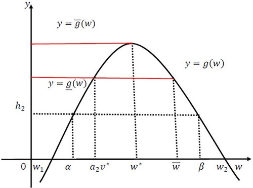We refer readers to Figure for the general features of fitness functions f and g.

Figure 1. Typical fitness functions for system (Equation1(1) ${\begin{aligned} \frac{d u_{j}}{d t} = d_{1} D_{2} [u_{j}] (t) + u_{j} (t) f (c_{11} u_{j} (t) + c_{12} v_{j} (t)) - h_{1} u_{j} (t), \\ \frac{d v_{j}}{d t} = d_{2} D_{2} [v_{j}] (t) + v_{j} (t) g (c_{21} u_{j} (t) + c_{22} v_{j} (t)) - h_{2} v_{j} (t), t \in R^{+}, j \in Z, \end{aligned}$ (1) ).

Figure 1. Typical fitness functions for system (Equation1(1) {dujdt=d1D2[uj](t)+uj(t)f(c11uj(t)+c12vj(t))−h1uj(t),dvjdt=d2D2[vj](t)+vj(t)g(c21uj(t)+c22vj(t))−h2vj(t), t∈R+, j∈Z,(1) ).

For the simplicity of notations, we consider the following non-dimensional system of (Equation1(1) ${\begin{aligned} \frac{d u_{j}}{d t} = d_{1} D_{2} [u_{j}] (t) + u_{j} (t) f (c_{11} u_{j} (t) + c_{12} v_{j} (t)) - h_{1} u_{j} (t), \\ \frac{d v_{j}}{d t} = d_{2} D_{2} [v_{j}] (t) + v_{j} (t) g (c_{21} u_{j} (t) + c_{22} v_{j} (t)) - h_{2} v_{j} (t), t \in R^{+}, j \in Z, \end{aligned}$ (1) ): (2) ${\begin{aligned} \frac{d u_{j}}{d t} = d_{1} D_{2} [u_{j}] (t) + u_{j} (t) f (a_{1} u_{j} (t) + v_{j} (t)) - h_{1} u_{j} (t), \\ \frac{d v_{j}}{d t} = d_{2} D_{2} [v_{j}] (t) + v_{j} (t) g (u_{j} (t) + a_{2} v_{j} (t)) - h_{2} v_{j} (t), \end{aligned}$ (2) which is obtained by the scaling $c_{21} u_{j} \to u_{j}, c_{12} v_{j} \to v_{j}, \frac{c_{11}}{c_{21}} \to a_{1}, \frac{c_{22}}{c_{12}} \to a_{2} .$ We are interested in situations that the system admits at least one positive equilibrium, thus we assume the following conditions hold: $0 \leq h_{1} < f (0), 0 \leq h_{2} < g (w^{*}) .$ It follows that there exist $0 < γ \leq z_{0}, 0 < w_{1} \leq α < β \leq w_{2}$ such that $f (γ) = h_{1}, g (α) = g (β) = h_{2} .$ By the properties of functions f and g, we calculate that system (Equation2(2) ${\begin{aligned} \frac{d u_{j}}{d t} = d_{1} D_{2} [u_{j}] (t) + u_{j} (t) f (a_{1} u_{j} (t) + v_{j} (t)) - h_{1} u_{j} (t), \\ \frac{d v_{j}}{d t} = d_{2} D_{2} [v_{j}] (t) + v_{j} (t) g (u_{j} (t) + a_{2} v_{j} (t)) - h_{2} v_{j} (t), \end{aligned}$ (2) ) always has the following axial equilibria $E_{0} = (0, 0), E_{1} = (0, \frac{α}{a_{2}}), E_{2} = (0, \frac{β}{a_{2}}), E_{3} = (\frac{γ}{a_{1}}, 0)$ and possibly two positive equilibria $E^{+} = (u^{+}, v^{+})$ and $E^{*} = (u^{*}, v^{*}),$ where $(u^{+}, v^{+})$ and $(u^{*}, v^{*})$ are the solutions of the algebraic equations ${\begin{aligned} a_{1} u + v = γ, \\ u + a_{2} v = α, \end{aligned} and {\begin{aligned} a_{1} u + v = γ, \\ u + a_{2} v = β, \end{aligned}$ respectively. Solving equations, we get $u^{+} = \frac{a_{2} γ - α}{a_{1} a_{2} - 1}, v^{+} = \frac{a_{1} α - γ}{a_{1} a_{2} - 1}, u^{*} = \frac{a_{2} γ - β}{a_{1} a_{2} - 1}, v^{*} = \frac{a_{1} β - γ}{a_{1} a_{2} - 1} .$ Note that the lattice model (Equation1(1) ${\begin{aligned} \frac{d u_{j}}{d t} = d_{1} D_{2} [u_{j}] (t) + u_{j} (t) f (c_{11} u_{j} (t) + c_{12} v_{j} (t)) - h_{1} u_{j} (t), \\ \frac{d v_{j}}{d t} = d_{2} D_{2} [v_{j}] (t) + v_{j} (t) g (c_{21} u_{j} (t) + c_{22} v_{j} (t)) - h_{2} v_{j} (t), t \in R^{+}, j \in Z, \end{aligned}$ (1) ) can be regarded as a discrete version of the corresponding reaction-diffusion pioneer-climax competition system in continuous habitats. Due to the rich dynamics of the pioneer-climax competition models, the spatiotemporal dynamics of the reaction-diffusion pioneer-climax systems has attracted a lot of attention from mathematicians and ecologists in the last few decades, see [Citation5,Citation7–11] and references therein. Most of these works focus on the existence of spreading speeds and travelling waves, and the bifurcation and Turing stability analysis also have been studied. However, up to our best knowledge, the study of the spatiotemporal dynamics of lattice pioneer-climax systems is quite few. In [Citation12], the authors first proposed the following delayed lattice pioneer-climax model: (3) ${\begin{aligned} \frac{d u_{j}}{d t} = d_{1} D_{2} [u_{j}] (t) + u_{j} (t) f (c_{11} u_{j} (t) + v_{j} (t - τ)), \\ \frac{d v_{j}}{d t} = d_{2} D_{2} [v_{j}] (t) + v_{j} (t) g (u_{j} (t) + c_{22} v_{j} (t - τ)), t \in R^{+}, j \in Z, \end{aligned}$ (3) where the parameter τ is interpreted by the interaction delay between two species. Under suitable assumptions so that the system (Equation3(3) ${\begin{aligned} \frac{d u_{j}}{d t} = d_{1} D_{2} [u_{j}] (t) + u_{j} (t) f (c_{11} u_{j} (t) + v_{j} (t - τ)), \\ \frac{d v_{j}}{d t} = d_{2} D_{2} [v_{j}] (t) + v_{j} (t) g (u_{j} (t) + c_{22} v_{j} (t - τ)), t \in R^{+}, j \in Z, \end{aligned}$ (3) ) is monotone in the competition order, the existence of monotone travelling waves connecting the pioneer-only boundary equilibrium to the co-existence positive equilibrium is studied. The result in [Citation12] shows that the interaction delay does not change the conditions under which the system admits the climax-invasion travelling waves, and the analysis is similar. Thus, to make the analytic writing clearly and easily understood for broader readers, we do not take the interaction delays into our model. It has been shown that the lattice differential equations are more suitable in modelling the population dynamics in the discrete habitat, and they could behave differently from the corresponding reaction-diffusion equations (see e.g. [Citation13,Citation14]), which motivates the study of this work.

Remark 1.1

We should point out that all results in this work are valid for the delayed version of (Equation1(1) ${\begin{aligned} \frac{d u_{j}}{d t} = d_{1} D_{2} [u_{j}] (t) + u_{j} (t) f (c_{11} u_{j} (t) + c_{12} v_{j} (t)) - h_{1} u_{j} (t), \\ \frac{d v_{j}}{d t} = d_{2} D_{2} [v_{j}] (t) + v_{j} (t) g (c_{21} u_{j} (t) + c_{22} v_{j} (t)) - h_{2} v_{j} (t), t \in R^{+}, j \in Z, \end{aligned}$ (1) ), which can be verified similarly by constructing two delayed auxiliary systems and using the similar upper-lower solution arguments as used in this paper.

The dynamics of the pioneer-climax interaction model (Equation2(2) ${\begin{aligned} \frac{d u_{j}}{d t} = d_{1} D_{2} [u_{j}] (t) + u_{j} (t) f (a_{1} u_{j} (t) + v_{j} (t)) - h_{1} u_{j} (t), \\ \frac{d v_{j}}{d t} = d_{2} D_{2} [v_{j}] (t) + v_{j} (t) g (u_{j} (t) + a_{2} v_{j} (t)) - h_{2} v_{j} (t), \end{aligned}$ (2) ) is quite rich and has not been understood well. Throughout of this work, we assume the parameters in (Equation2(2) ${\begin{aligned} \frac{d u_{j}}{d t} = d_{1} D_{2} [u_{j}] (t) + u_{j} (t) f (a_{1} u_{j} (t) + v_{j} (t)) - h_{1} u_{j} (t), \\ \frac{d v_{j}}{d t} = d_{2} D_{2} [v_{j}] (t) + v_{j} (t) g (u_{j} (t) + a_{2} v_{j} (t)) - h_{2} v_{j} (t), \end{aligned}$ (2) ) satisfying the following assumption (H1) or (H2):

(H1)	$γ > \frac{β}{a_{2}}, β > \frac{γ}{a_{1}} > α;$
(H2)	$γ > \frac{β}{a_{2}}, α > \frac{γ}{a_{1}}$ .

In the case of (H1), (Equation2(2) ${\begin{aligned} \frac{d u_{j}}{d t} = d_{1} D_{2} [u_{j}] (t) + u_{j} (t) f (a_{1} u_{j} (t) + v_{j} (t)) - h_{1} u_{j} (t), \\ \frac{d v_{j}}{d t} = d_{2} D_{2} [v_{j}] (t) + v_{j} (t) g (u_{j} (t) + a_{2} v_{j} (t)) - h_{2} v_{j} (t), \end{aligned}$ (2) ) admits the unique stable coexistence equilibrium $E^{*}$ . While under (H2), in addition to stable coexistence equilibrium $E^{*}$ , (Equation2(2) ${\begin{aligned} \frac{d u_{j}}{d t} = d_{1} D_{2} [u_{j}] (t) + u_{j} (t) f (a_{1} u_{j} (t) + v_{j} (t)) - h_{1} u_{j} (t), \\ \frac{d v_{j}}{d t} = d_{2} D_{2} [v_{j}] (t) + v_{j} (t) g (u_{j} (t) + a_{2} v_{j} (t)) - h_{2} v_{j} (t), \end{aligned}$ (2) ) has the other coexistence equilibrium $E^{+} .$ For the location of equilibria of (Equation2(2) ${\begin{aligned} \frac{d u_{j}}{d t} = d_{1} D_{2} [u_{j}] (t) + u_{j} (t) f (a_{1} u_{j} (t) + v_{j} (t)) - h_{1} u_{j} (t), \\ \frac{d v_{j}}{d t} = d_{2} D_{2} [v_{j}] (t) + v_{j} (t) g (u_{j} (t) + a_{2} v_{j} (t)) - h_{2} v_{j} (t), \end{aligned}$ (2) ) under (H1) or (H2), we refer readers to Figure (a) and (b), respectively. Under (H1) or (H2), it is easy to check that $a_{1} a_{2} > 1$ . Moreover, we observe from Figure that $u^{*} < \frac{γ}{a_{1}}$ and $v^{*} < \frac{β}{a_{2}}$ hold for both cases. For the rich dynamics and a complete categorization of the stability of the equilibria of the spatially homogeneous system (ordinary differential system) of (Equation2(2) ${\begin{aligned} \frac{d u_{j}}{d t} = d_{1} D_{2} [u_{j}] (t) + u_{j} (t) f (a_{1} u_{j} (t) + v_{j} (t)) - h_{1} u_{j} (t), \\ \frac{d v_{j}}{d t} = d_{2} D_{2} [v_{j}] (t) + v_{j} (t) g (u_{j} (t) + a_{2} v_{j} (t)) - h_{2} v_{j} (t), \end{aligned}$ (2) ), we refer readers to [Citation3,Citation4,Citation15–18] and references therein.

Figure 2. Nullclines and the structure of equilibria of (Equation2(2) ${\begin{aligned} \frac{d u_{j}}{d t} = d_{1} D_{2} [u_{j}] (t) + u_{j} (t) f (a_{1} u_{j} (t) + v_{j} (t)) - h_{1} u_{j} (t), \\ \frac{d v_{j}}{d t} = d_{2} D_{2} [v_{j}] (t) + v_{j} (t) g (u_{j} (t) + a_{2} v_{j} (t)) - h_{2} v_{j} (t), \end{aligned}$ (2) ) with (H1) and (H2).

Figure 2. Nullclines and the structure of equilibria of (Equation2(2) {dujdt=d1D2[uj](t)+uj(t)f(a1uj(t)+vj(t))−h1uj(t),dvjdt=d2D2[vj](t)+vj(t)g(uj(t)+a2vj(t))−h2vj(t),(2) ) with (H1) and (H2).

In the remainder of this work, we further assume the parameters in (Equation2(2) ${\begin{aligned} \frac{d u_{j}}{d t} = d_{1} D_{2} [u_{j}] (t) + u_{j} (t) f (a_{1} u_{j} (t) + v_{j} (t)) - h_{1} u_{j} (t), \\ \frac{d v_{j}}{d t} = d_{2} D_{2} [v_{j}] (t) + v_{j} (t) g (u_{j} (t) + a_{2} v_{j} (t)) - h_{2} v_{j} (t), \end{aligned}$ (2) ) satisfy the following condition:

(A1)

$\frac{α}{a_{2}} < v^{*} < \frac{w^{*}}{a_{2}}$ .

From Figure , we observe that (Equation2) has no other equilibrium located in the rectangle with two opposite vertices

E_{2}

and

E^{*}

. Moreover, the results in [Citation4] show that, under (H1) or (H2), the positive equilibrium

E^{*}

is attractive in the interior of the rectangle. Under conditions (H1)-(A1) or (H2)-(A1), the fitness function g is no longer monotone decreasing for some population densities, so the system is nonmonotone in the competition order. Motivated by the recent work [Citation11], we will appeal to the sandwich technique to determine the existence of the spreading speed and travelling waves. Moreover, the linear selection of the spreading speed is investigated by constructing suitable upper solutions. As far as we know, the invasion dynamics of the lattice model (Equation2) under conditions (H1)-(A1) or (H2)-(A1) has not been studied in the literature.

Remark 1.2

The interpretation of (H1) could be observed from the intersection points of the uv axes with nuclines from Figure (a). It determines the location of nuclines, and guarantees the stability of positive equilibrium $E^{*}$ . Similarly, the interpretation of (H2) could be observed from Figure (b). The condition (A1) is a technical assumption which is needed to make the theoretical analysis tractable.

The purpose of this work is to estimate the spreading speeds, and determine the existence of travelling waves of (Equation2(2) ${\begin{aligned} \frac{d u_{j}}{d t} = d_{1} D_{2} [u_{j}] (t) + u_{j} (t) f (a_{1} u_{j} (t) + v_{j} (t)) - h_{1} u_{j} (t), \\ \frac{d v_{j}}{d t} = d_{2} D_{2} [v_{j}] (t) + v_{j} (t) g (u_{j} (t) + a_{2} v_{j} (t)) - h_{2} v_{j} (t), \end{aligned}$ (2) ) connecting $E_{2}$ to $E^{*}$ . Note that (Equation2(2) ${\begin{aligned} \frac{d u_{j}}{d t} = d_{1} D_{2} [u_{j}] (t) + u_{j} (t) f (a_{1} u_{j} (t) + v_{j} (t)) - h_{1} u_{j} (t), \\ \frac{d v_{j}}{d t} = d_{2} D_{2} [v_{j}] (t) + v_{j} (t) g (u_{j} (t) + a_{2} v_{j} (t)) - h_{2} v_{j} (t), \end{aligned}$ (2) ) is not a standard competition system, and the comparison principle does not satisfy for some parameters, which makes the model analysis complicated. With (H1) and the assumption $w^{*} \leq u^{*}$ so that the system is monotone for the densities bounded by $E_{3}$ and $E^{*}$ , the authors in [Citation12] proved the existence of travelling waves of (Equation3(3) ${\begin{aligned} \frac{d u_{j}}{d t} = d_{1} D_{2} [u_{j}] (t) + u_{j} (t) f (c_{11} u_{j} (t) + v_{j} (t - τ)), \\ \frac{d v_{j}}{d t} = d_{2} D_{2} [v_{j}] (t) + v_{j} (t) g (u_{j} (t) + c_{22} v_{j} (t - τ)), t \in R^{+}, j \in Z, \end{aligned}$ (3) ) connecting $E_{3}$ to $E^{*}$ , where the monotonicity of the system and the fixed point theorem are used. However, under (H1)-(A1) or (H2)-(A1), the system (Equation2(2) ${\begin{aligned} \frac{d u_{j}}{d t} = d_{1} D_{2} [u_{j}] (t) + u_{j} (t) f (a_{1} u_{j} (t) + v_{j} (t)) - h_{1} u_{j} (t), \\ \frac{d v_{j}}{d t} = d_{2} D_{2} [v_{j}] (t) + v_{j} (t) g (u_{j} (t) + a_{2} v_{j} (t)) - h_{2} v_{j} (t), \end{aligned}$ (2) ) is no longer monotone for population densities between $E_{2}$ and $E^{*}$ , for which the method and arguments used in [Citation12] cannot be applied similarly. We construct two auxiliary systems and appeal to comparison arguments to estimate the population spreading speeds. Moreover, the linear selection of the spreading speed is established by constructing suitable upper solutions. To prove the existence of travelling waves of (Equation2(2) ${\begin{aligned} \frac{d u_{j}}{d t} = d_{1} D_{2} [u_{j}] (t) + u_{j} (t) f (a_{1} u_{j} (t) + v_{j} (t)) - h_{1} u_{j} (t), \\ \frac{d v_{j}}{d t} = d_{2} D_{2} [v_{j}] (t) + v_{j} (t) g (u_{j} (t) + a_{2} v_{j} (t)) - h_{2} v_{j} (t), \end{aligned}$ (2) ) connecting $E_{2}$ to $E^{*}$ , we construct new upper and lower solutions which are essentially different with those used in [Citation12]. It is well known that the asymptotic behaviour of travelling waves for non-monotone system is technically difficult since the travelling waves solutions may be non-monotone. To overcome this difficulty, we use the travelling wave solutions of the lower auxiliary system as the lower solutions of the non-monotone system (Equation2(2) ${\begin{aligned} \frac{d u_{j}}{d t} = d_{1} D_{2} [u_{j}] (t) + u_{j} (t) f (a_{1} u_{j} (t) + v_{j} (t)) - h_{1} u_{j} (t), \\ \frac{d v_{j}}{d t} = d_{2} D_{2} [v_{j}] (t) + v_{j} (t) g (u_{j} (t) + a_{2} v_{j} (t)) - h_{2} v_{j} (t), \end{aligned}$ (2) ), then we show that the established travelling wave solutions could connect $E_{2}$ to $E^{*}$ . To the best of our knowledge, our results are new to study the linear selection of the spreading speed of non-monotone lattice pioneer-climax interaction models.

The rest of this paper is organized as follows. In Section 2, we present the preliminaries and show the well-posedness of the initial value problem. In Section 3, we estimate the spreading speed of populations, and figure out the conditions under which the system admits linearly selected spreading speeds. In Section 4, with the assumption that $d_{1} \geq d_{2}$ , we establish the existence of travelling wave solutions of (Equation2(2) ${\begin{aligned} \frac{d u_{j}}{d t} = d_{1} D_{2} [u_{j}] (t) + u_{j} (t) f (a_{1} u_{j} (t) + v_{j} (t)) - h_{1} u_{j} (t), \\ \frac{d v_{j}}{d t} = d_{2} D_{2} [v_{j}] (t) + v_{j} (t) g (u_{j} (t) + a_{2} v_{j} (t)) - h_{2} v_{j} (t), \end{aligned}$ (2) ) connecting $E_{2}$ to $E^{*}$ , and show that the minimum wave speed is coincident with the spreading speed. At the end of this work, we apply our theoretical results to a lattice pioneer-climax model with linear decreasing pioneer fitness and quadratic climax fitness functions, then some discussions finish this paper.

2. Preliminaries

Let $B := {ϕ = {ϕ_{j}}_{j \in Z} : ϕ_{j} \in R^{2}}$ be the space of all uniformly bounded functions from $Z$ to $R^{2}$ . We equip $B$ with the compact open topology, that is, a sequence $ϕ^{n}$ converges to ϕ in $C$ if $ϕ_{j}^{n}$ converges to $ϕ_{j}$ in $R^{2}$ uniformly for j in any compact subset of $Z$ . This topology can be induced by the following norm: $‖ ϕ ‖_{B} := \sum_{k = 1}^{\infty} \frac{1}{2^{k}} max_{j \in [- k, k]} | ϕ_{j} |, \forall ϕ \in B .$ Then $(C, ‖ \cdot ‖_{B})$ is a normed space. For any vectors $a, b$ in $R^{2}$ , we define $b \geq (>) a$ if $b - a \in R_{+}^{2} (R_{+}^{2} ∖ {0})$ , and $b ≫ a$ if $b - a \in int (R_{+}^{2})$ . Let $B_{+} := {ϕ \in B : ϕ (j) \geq 0, j \in Z}$ . Then $B_{+}$ is a nonempty closed cone of $B$ and induces the standard pointwise ordering in $B$ . Denote $X := BC (R, R^{2})$ to be the set of all bounded and continuous functions from $R$ to $R^{2}$ . Then $X_{+}$ and the corresponding ordering in $X$ can be defined similarly. For any $b = (b_{1}, b_{2}) \in int (R_{+}^{2})$ , we define $[0, b] := {(x, y) \in R_{+}^{2} : 0 \leq (x, y) \leq b}$ , $B_{b} := {ϕ \in B : 0 \leq ϕ_{j} \leq b, \forall j \in Z}$ , and $X_{b} := {ψ \in X : 0 \leq ψ (x) \leq b, \forall x \in R}$ .

For the convenience of mathematical analysis, we make the change of variables ${\tilde{u}}_{j} = u_{j}$ and ${\tilde{v}}_{j} = \frac{β}{a_{2}} - v_{j}$ and drop the tildes, then (Equation2(2) ${\begin{aligned} \frac{d u_{j}}{d t} = d_{1} D_{2} [u_{j}] (t) + u_{j} (t) f (a_{1} u_{j} (t) + v_{j} (t)) - h_{1} u_{j} (t), \\ \frac{d v_{j}}{d t} = d_{2} D_{2} [v_{j}] (t) + v_{j} (t) g (u_{j} (t) + a_{2} v_{j} (t)) - h_{2} v_{j} (t), \end{aligned}$ (2) ) converts to the following system (4) ${\begin{aligned} \frac{d u_{j}}{d t} = d_{1} D_{2} [u_{j}] (t) + u_{j} (t) f (\frac{β}{a_{2}} + a_{1} u_{j} (t) - v_{j} (t)) - h_{1} u_{j} (t), \\ \frac{d v_{j}}{d t} = d_{2} D_{2} [v_{j}] (t) - (\frac{β}{a_{2}} - v_{j} (t)) g (β + u_{j} (t) - a_{2} v_{j} (t)) + h_{2} (\frac{β}{a_{2}} - v_{j} (t)), \end{aligned}$ (4) and the equilibria $E_{2}$ and $E^{*}$ of (Equation2(2) ${\begin{aligned} \frac{d u_{j}}{d t} = d_{1} D_{2} [u_{j}] (t) + u_{j} (t) f (a_{1} u_{j} (t) + v_{j} (t)) - h_{1} u_{j} (t), \\ \frac{d v_{j}}{d t} = d_{2} D_{2} [v_{j}] (t) + v_{j} (t) g (u_{j} (t) + a_{2} v_{j} (t)) - h_{2} v_{j} (t), \end{aligned}$ (2) ) correspond to $E_{2} = (0, 0), E^{*} = (u^{*}, \frac{β}{a_{2}} - v^{*}),$ for (Equation4(4) ${\begin{aligned} \frac{d u_{j}}{d t} = d_{1} D_{2} [u_{j}] (t) + u_{j} (t) f (\frac{β}{a_{2}} + a_{1} u_{j} (t) - v_{j} (t)) - h_{1} u_{j} (t), \\ \frac{d v_{j}}{d t} = d_{2} D_{2} [v_{j}] (t) - (\frac{β}{a_{2}} - v_{j} (t)) g (β + u_{j} (t) - a_{2} v_{j} (t)) + h_{2} (\frac{β}{a_{2}} - v_{j} (t)), \end{aligned}$ (4) ), respectively. Note that $E_{2} ≪ E^{*}$ and there exists no other equilibrium between them. We are interested in the existence of the spreading speed and travelling waves of (Equation4(4) ${\begin{aligned} \frac{d u_{j}}{d t} = d_{1} D_{2} [u_{j}] (t) + u_{j} (t) f (\frac{β}{a_{2}} + a_{1} u_{j} (t) - v_{j} (t)) - h_{1} u_{j} (t), \\ \frac{d v_{j}}{d t} = d_{2} D_{2} [v_{j}] (t) - (\frac{β}{a_{2}} - v_{j} (t)) g (β + u_{j} (t) - a_{2} v_{j} (t)) + h_{2} (\frac{β}{a_{2}} - v_{j} (t)), \end{aligned}$ (4) ) connecting $E_{2}$ to $E^{*}$ . Let $w = (u, v)^{T} \in B_{+}$ with $w_{j} = (u_{j}, v_{j})^{T}, j \in Z$ . Define $F = (F_{1}, F_{2})^{T} : B_{+} \to B$ by $\begin{aligned} F_{1} [w] (j) & := u_{j} f (\frac{β}{a_{2}} + a_{1} u_{j} - v_{j}) - h_{1} u_{j}, \\ F_{2} [w] (j) & := - (\frac{β}{a_{2}} - v_{j}) g (β + u_{j} - a_{2} v_{j}) + h_{2} (\frac{β}{a_{2}} - v_{j}) . \end{aligned}$ Let $A : B \to B$ be defined as $A [w] (j) := (d_{1} D_{2} [u_{j}], d_{2} D_{2} [v_{j}])^{T}$ . Then system (Equation4(4) ${\begin{aligned} \frac{d u_{j}}{d t} = d_{1} D_{2} [u_{j}] (t) + u_{j} (t) f (\frac{β}{a_{2}} + a_{1} u_{j} (t) - v_{j} (t)) - h_{1} u_{j} (t), \\ \frac{d v_{j}}{d t} = d_{2} D_{2} [v_{j}] (t) - (\frac{β}{a_{2}} - v_{j} (t)) g (β + u_{j} (t) - a_{2} v_{j} (t)) + h_{2} (\frac{β}{a_{2}} - v_{j} (t)), \end{aligned}$ (4) ) can be written as the following general form: (5) $\frac{d w}{d t} = A [w (t)] + F [w (t)] .$ (5) Let ${S (t)}_{t \geq 0}$ be the solution semigroup associated with the following linear lattice differential equations: $\frac{d u_{j}}{d t} = u_{j + 1} (t) + u_{j - 1} (t) - 2 u_{j} (t), t > 0, j \in Z,$ which was given in [Citation19, Section 2] by the modified Bessel functions as follows: $S (t) [w_{0}] (j) = e^{- 2 t} \sum_{i = - \infty}^{\infty} I_{i} (2 t) w_{0} (j - i), \forall w_{0} \in B, t > 0,$ where $I_{i}, i \geq 0$ are given by $I_{i} (t) = \sum_{k = 0}^{\infty} \frac{{(\frac{t}{2})}^{i + 2 k}}{k! (i + k)!},$ and $I_{i} (t) = I_{- i} (t)$ for i<0. Note that $S (t) B_{+} \subseteq B_{+}$ for any $t \geq 0$ . Set $P (t) := diag (S (d_{1} t), S (d_{2} t))$ . It follows from [Citation19, Remark 2.6] that system (Equation5(5) $\frac{d w}{d t} = A [w (t)] + F [w (t)] .$ (5) ) with initial data $w_{0} \in B$ can be written as the following integral equation: (6) $w (t) = P (t) [w_{0}] + \int_{0}^{t} P (t - s) F [w (s)] d s, \forall t \geq 0.$ (6)

Definition 2.1

A solution $w (t)$ of (Equation6(6) $w (t) = P (t) [w_{0}] + \int_{0}^{t} P (t - s) F [w (s)] d s, \forall t \geq 0.$ (6) ) is said to be a mild solution of (Equation4(4) ${\begin{aligned} \frac{d u_{j}}{d t} = d_{1} D_{2} [u_{j}] (t) + u_{j} (t) f (\frac{β}{a_{2}} + a_{1} u_{j} (t) - v_{j} (t)) - h_{1} u_{j} (t), \\ \frac{d v_{j}}{d t} = d_{2} D_{2} [v_{j}] (t) - (\frac{β}{a_{2}} - v_{j} (t)) g (β + u_{j} (t) - a_{2} v_{j} (t)) + h_{2} (\frac{β}{a_{2}} - v_{j} (t)), \end{aligned}$ (4) ), and a function $\bar{w} : R_{+} \to B$ is called an upper (a lower) solution of (Equation4(4) ${\begin{aligned} \frac{d u_{j}}{d t} = d_{1} D_{2} [u_{j}] (t) + u_{j} (t) f (\frac{β}{a_{2}} + a_{1} u_{j} (t) - v_{j} (t)) - h_{1} u_{j} (t), \\ \frac{d v_{j}}{d t} = d_{2} D_{2} [v_{j}] (t) - (\frac{β}{a_{2}} - v_{j} (t)) g (β + u_{j} (t) - a_{2} v_{j} (t)) + h_{2} (\frac{β}{a_{2}} - v_{j} (t)), \end{aligned}$ (4) ) if it satisfies (7) $\bar{w} (t) \geq (\leq) P (t) [\bar{w} (0)] + \int_{0}^{t} P (t - s) F [\bar{w} (s)] d s, \forall t \geq 0.$ (7)

By the standard contracting mapping theorem arguments (see e.g. [Citation20, Theorem 4.2]), we have the following well-posedness result for the initial-value problem.

Lemma 2.2

Assume that (H1)-(A1) or (H2)-(A1) hold. Then for any given $w_{0} \in B_{E^{*}}$ , system (Equation4(4) ${\begin{aligned} \frac{d u_{j}}{d t} = d_{1} D_{2} [u_{j}] (t) + u_{j} (t) f (\frac{β}{a_{2}} + a_{1} u_{j} (t) - v_{j} (t)) - h_{1} u_{j} (t), \\ \frac{d v_{j}}{d t} = d_{2} D_{2} [v_{j}] (t) - (\frac{β}{a_{2}} - v_{j} (t)) g (β + u_{j} (t) - a_{2} v_{j} (t)) + h_{2} (\frac{β}{a_{2}} - v_{j} (t)), \end{aligned}$ (4) ) has a unique mild solution $w (t) = {w_{j} (t)}_{j \in Z}$ with $w (0) = w_{0}$ , and $w (t) \in B_{E^{*}}$ for any t>0.

Now we present the definition of the invasion spreading speed and travelling waves of (Equation4(4) ${\begin{aligned} \frac{d u_{j}}{d t} = d_{1} D_{2} [u_{j}] (t) + u_{j} (t) f (\frac{β}{a_{2}} + a_{1} u_{j} (t) - v_{j} (t)) - h_{1} u_{j} (t), \\ \frac{d v_{j}}{d t} = d_{2} D_{2} [v_{j}] (t) - (\frac{β}{a_{2}} - v_{j} (t)) g (β + u_{j} (t) - a_{2} v_{j} (t)) + h_{2} (\frac{β}{a_{2}} - v_{j} (t)), \end{aligned}$ (4) ) connecting equilibria $E_{2}$ and $E^{*}$ .

Definition 2.3

A number $c^{*} > 0$ is called the spreading speed of (Equation4(4) ${\begin{aligned} \frac{d u_{j}}{d t} = d_{1} D_{2} [u_{j}] (t) + u_{j} (t) f (\frac{β}{a_{2}} + a_{1} u_{j} (t) - v_{j} (t)) - h_{1} u_{j} (t), \\ \frac{d v_{j}}{d t} = d_{2} D_{2} [v_{j}] (t) - (\frac{β}{a_{2}} - v_{j} (t)) g (β + u_{j} (t) - a_{2} v_{j} (t)) + h_{2} (\frac{β}{a_{2}} - v_{j} (t)), \end{aligned}$ (4) ) if the solution $w (t) = {(u_{j} (t), v_{j} (t))}_{j \in Z}$ with the initial data $w_{0} = {(u_{j, 0}, v_{j, 0})}_{j \in Z} \in B_{E^{*}}$ satisfies the following statements:

For any $c > c^{*}$ , if $u_{j, 0} = v_{j, 0} = 0, | j | \geq k$ for some k>0, then $lim_{t \to \infty, | j | \geq ct} (u_{j} (t), v_{j} (t)) = E_{2};$
For any $0 < c < c^{*}$ and $σ \in [0, E^{*}]$ with $σ ≫ 0$ , if there is a positive number $r_{σ}$ such that $(u_{j, 0}, v_{j, 0}) ≫ σ$ for j on an interval of length $2 r_{σ}$ , then $lim_{t \to \infty, | j | \leq ct} (u_{j} (t), v_{j} (t)) = E^{*} .$

Definition 2.4

A travelling wave solution of (Equation4(4) ${\begin{aligned} \frac{d u_{j}}{d t} = d_{1} D_{2} [u_{j}] (t) + u_{j} (t) f (\frac{β}{a_{2}} + a_{1} u_{j} (t) - v_{j} (t)) - h_{1} u_{j} (t), \\ \frac{d v_{j}}{d t} = d_{2} D_{2} [v_{j}] (t) - (\frac{β}{a_{2}} - v_{j} (t)) g (β + u_{j} (t) - a_{2} v_{j} (t)) + h_{2} (\frac{β}{a_{2}} - v_{j} (t)), \end{aligned}$ (4) ) connecting $E_{2}$ to $E^{*}$ is a continuous solution of (Equation4(4) ${\begin{aligned} \frac{d u_{j}}{d t} = d_{1} D_{2} [u_{j}] (t) + u_{j} (t) f (\frac{β}{a_{2}} + a_{1} u_{j} (t) - v_{j} (t)) - h_{1} u_{j} (t), \\ \frac{d v_{j}}{d t} = d_{2} D_{2} [v_{j}] (t) - (\frac{β}{a_{2}} - v_{j} (t)) g (β + u_{j} (t) - a_{2} v_{j} (t)) + h_{2} (\frac{β}{a_{2}} - v_{j} (t)), \end{aligned}$ (4) ) with the form $(u_{j} (t), v_{j} (t)) = (U (j + ct), V (j + ct))$ and the following asymptotic boundary conditions hold: (8) $(U (- \infty), V (- \infty)) = E_{2}, (U (\infty), V (\infty)) = E^{*} .$ (8) The constant c>0 is called the wave speed, and the functions U, V are called the wave profiles.

3. The spreading speed

In this section, we study the spreading speed of (Equation2(2) ${\begin{aligned} \frac{d u_{j}}{d t} = d_{1} D_{2} [u_{j}] (t) + u_{j} (t) f (a_{1} u_{j} (t) + v_{j} (t)) - h_{1} u_{j} (t), \\ \frac{d v_{j}}{d t} = d_{2} D_{2} [v_{j}] (t) + v_{j} (t) g (u_{j} (t) + a_{2} v_{j} (t)) - h_{2} v_{j} (t), \end{aligned}$ (2) ) under nonmonotone conditions (H1)-(A1) or (H2)-(A1). In order to use the sandwich technique, we first construct suitable upper and lower auxiliary systems for (Equation4(4) ${\begin{aligned} \frac{d u_{j}}{d t} = d_{1} D_{2} [u_{j}] (t) + u_{j} (t) f (\frac{β}{a_{2}} + a_{1} u_{j} (t) - v_{j} (t)) - h_{1} u_{j} (t), \\ \frac{d v_{j}}{d t} = d_{2} D_{2} [v_{j}] (t) - (\frac{β}{a_{2}} - v_{j} (t)) g (β + u_{j} (t) - a_{2} v_{j} (t)) + h_{2} (\frac{β}{a_{2}} - v_{j} (t)), \end{aligned}$ (4) ).

3.1. The estimation of spreading speeds

From (A1), we know that $α < a_{2} v^{*} < w^{*}$ . Note that the function g is hump-shaped satisfying $g (α) = g (β)$ , and gets its maximum value at $w^{*}$ . Then there exists a unique $\bar{w} \in (w^{*}, β)$ such that $g (a_{2} v^{*}) = g (\bar{w})$ . Now we define two auxiliary functions $\bar{g} (w) = {\begin{aligned} g (w^{*}), & w \leq w^{*}, \\ g (w), & w > w^{*}, \end{aligned} \underline{g} (w) = {\begin{aligned} g (a_{2} v^{*}), & w \leq \bar{w}, \\ g (w), & w > \bar{w} . \end{aligned}$ We refer readers to Figure for the construction of $\bar{g}$ and $\underline{g}$ under the condition (A1). Then both $\bar{g}$ and $\underline{g}$ are decreasing and satisfy (9) $\begin{aligned} \bar{g} (w) & \geq g (w) \geq \underline{g} (w), for w \geq a_{2} v^{*}, \\ \bar{g} (w) & = \underline{g} (w) = g (w), for w \geq \bar{w} . \end{aligned}$ (9) Then we define an upper system of (Equation4(4) ${\begin{aligned} \frac{d u_{j}}{d t} = d_{1} D_{2} [u_{j}] (t) + u_{j} (t) f (\frac{β}{a_{2}} + a_{1} u_{j} (t) - v_{j} (t)) - h_{1} u_{j} (t), \\ \frac{d v_{j}}{d t} = d_{2} D_{2} [v_{j}] (t) - (\frac{β}{a_{2}} - v_{j} (t)) g (β + u_{j} (t) - a_{2} v_{j} (t)) + h_{2} (\frac{β}{a_{2}} - v_{j} (t)), \end{aligned}$ (4) ) with function $\underline{g}$ by (10) ${\begin{aligned} \frac{d u_{j}}{d t} = d_{1} D_{2} [u_{j}] (t) + u_{j} (t) f (\frac{β}{a_{2}} + a_{1} u_{j} (t) - v_{j} (t)) - h_{1} u_{j} (t), \\ \frac{d v_{j}}{d t} = d_{2} D_{2} [v_{j}] (t) - (\frac{β}{a_{2}} - v_{j} (t)) \underline{g} (β + u_{j} (t) - a_{2} v_{j} (t)) + h_{2} (\frac{β}{a_{2}} - v_{j} (t)), \end{aligned}$ (10) and a lower system of (Equation4(4) ${\begin{aligned} \frac{d u_{j}}{d t} = d_{1} D_{2} [u_{j}] (t) + u_{j} (t) f (\frac{β}{a_{2}} + a_{1} u_{j} (t) - v_{j} (t)) - h_{1} u_{j} (t), \\ \frac{d v_{j}}{d t} = d_{2} D_{2} [v_{j}] (t) - (\frac{β}{a_{2}} - v_{j} (t)) g (β + u_{j} (t) - a_{2} v_{j} (t)) + h_{2} (\frac{β}{a_{2}} - v_{j} (t)), \end{aligned}$ (4) ) with function $\bar{g}$ by (11) ${\begin{aligned} \frac{d u_{j}}{d t} = d_{1} D_{2} [u_{j}] (t) + u_{j} (t) f (\frac{β}{a_{2}} + a_{1} u_{j} (t) - v_{j} (t)) - h_{1} u_{j} (t), \\ \frac{d v_{j}}{d t} = d_{2} D_{2} [v_{j}] (t) - (\frac{β}{a_{2}} - v_{j} (t)) \bar{g} (β + u_{j} (t) - a_{2} v_{j} (t)) + h_{2} (\frac{β}{a_{2}} - v_{j} (t)), \end{aligned}$ (11) By a simple calculation, we know that $E_{2}$ and $E^{*}$ are equilibria of (Equation10(10) ${\begin{aligned} \frac{d u_{j}}{d t} = d_{1} D_{2} [u_{j}] (t) + u_{j} (t) f (\frac{β}{a_{2}} + a_{1} u_{j} (t) - v_{j} (t)) - h_{1} u_{j} (t), \\ \frac{d v_{j}}{d t} = d_{2} D_{2} [v_{j}] (t) - (\frac{β}{a_{2}} - v_{j} (t)) \underline{g} (β + u_{j} (t) - a_{2} v_{j} (t)) + h_{2} (\frac{β}{a_{2}} - v_{j} (t)), \end{aligned}$ (10) ) and (Equation11(11) ${\begin{aligned} \frac{d u_{j}}{d t} = d_{1} D_{2} [u_{j}] (t) + u_{j} (t) f (\frac{β}{a_{2}} + a_{1} u_{j} (t) - v_{j} (t)) - h_{1} u_{j} (t), \\ \frac{d v_{j}}{d t} = d_{2} D_{2} [v_{j}] (t) - (\frac{β}{a_{2}} - v_{j} (t)) \bar{g} (β + u_{j} (t) - a_{2} v_{j} (t)) + h_{2} (\frac{β}{a_{2}} - v_{j} (t)), \end{aligned}$ (11) ), and also there is no other equilibrium between them. Moreover, due to the monotonicity of $\underline{g}$ and $\bar{g}$ , we know that both (Equation10(10) ${\begin{aligned} \frac{d u_{j}}{d t} = d_{1} D_{2} [u_{j}] (t) + u_{j} (t) f (\frac{β}{a_{2}} + a_{1} u_{j} (t) - v_{j} (t)) - h_{1} u_{j} (t), \\ \frac{d v_{j}}{d t} = d_{2} D_{2} [v_{j}] (t) - (\frac{β}{a_{2}} - v_{j} (t)) \underline{g} (β + u_{j} (t) - a_{2} v_{j} (t)) + h_{2} (\frac{β}{a_{2}} - v_{j} (t)), \end{aligned}$ (10) ) and (Equation11(11) ${\begin{aligned} \frac{d u_{j}}{d t} = d_{1} D_{2} [u_{j}] (t) + u_{j} (t) f (\frac{β}{a_{2}} + a_{1} u_{j} (t) - v_{j} (t)) - h_{1} u_{j} (t), \\ \frac{d v_{j}}{d t} = d_{2} D_{2} [v_{j}] (t) - (\frac{β}{a_{2}} - v_{j} (t)) \bar{g} (β + u_{j} (t) - a_{2} v_{j} (t)) + h_{2} (\frac{β}{a_{2}} - v_{j} (t)), \end{aligned}$ (11) ) are cooperative in $B_{E^{*}}$ , and their solution semiflows are order-preserving. Moreover, we observe that the following comparison principle for the solutions of (Equation4(4) ${\begin{aligned} \frac{d u_{j}}{d t} = d_{1} D_{2} [u_{j}] (t) + u_{j} (t) f (\frac{β}{a_{2}} + a_{1} u_{j} (t) - v_{j} (t)) - h_{1} u_{j} (t), \\ \frac{d v_{j}}{d t} = d_{2} D_{2} [v_{j}] (t) - (\frac{β}{a_{2}} - v_{j} (t)) g (β + u_{j} (t) - a_{2} v_{j} (t)) + h_{2} (\frac{β}{a_{2}} - v_{j} (t)), \end{aligned}$ (4) ), (Equation10(10) ${\begin{aligned} \frac{d u_{j}}{d t} = d_{1} D_{2} [u_{j}] (t) + u_{j} (t) f (\frac{β}{a_{2}} + a_{1} u_{j} (t) - v_{j} (t)) - h_{1} u_{j} (t), \\ \frac{d v_{j}}{d t} = d_{2} D_{2} [v_{j}] (t) - (\frac{β}{a_{2}} - v_{j} (t)) \underline{g} (β + u_{j} (t) - a_{2} v_{j} (t)) + h_{2} (\frac{β}{a_{2}} - v_{j} (t)), \end{aligned}$ (10) ), and (Equation11(11) ${\begin{aligned} \frac{d u_{j}}{d t} = d_{1} D_{2} [u_{j}] (t) + u_{j} (t) f (\frac{β}{a_{2}} + a_{1} u_{j} (t) - v_{j} (t)) - h_{1} u_{j} (t), \\ \frac{d v_{j}}{d t} = d_{2} D_{2} [v_{j}] (t) - (\frac{β}{a_{2}} - v_{j} (t)) \bar{g} (β + u_{j} (t) - a_{2} v_{j} (t)) + h_{2} (\frac{β}{a_{2}} - v_{j} (t)), \end{aligned}$ (11) ) is valid.

Lemma 3.1

Assume that (H1)-(A1) or (H2)-(A1) hold. Let $w (t)$ , $w_{+} (t)$ and $w_{-} (t)$ be the solutions of (Equation4(4) ${\begin{aligned} \frac{d u_{j}}{d t} = d_{1} D_{2} [u_{j}] (t) + u_{j} (t) f (\frac{β}{a_{2}} + a_{1} u_{j} (t) - v_{j} (t)) - h_{1} u_{j} (t), \\ \frac{d v_{j}}{d t} = d_{2} D_{2} [v_{j}] (t) - (\frac{β}{a_{2}} - v_{j} (t)) g (β + u_{j} (t) - a_{2} v_{j} (t)) + h_{2} (\frac{β}{a_{2}} - v_{j} (t)), \end{aligned}$ (4) ), (Equation10(10) ${\begin{aligned} \frac{d u_{j}}{d t} = d_{1} D_{2} [u_{j}] (t) + u_{j} (t) f (\frac{β}{a_{2}} + a_{1} u_{j} (t) - v_{j} (t)) - h_{1} u_{j} (t), \\ \frac{d v_{j}}{d t} = d_{2} D_{2} [v_{j}] (t) - (\frac{β}{a_{2}} - v_{j} (t)) \underline{g} (β + u_{j} (t) - a_{2} v_{j} (t)) + h_{2} (\frac{β}{a_{2}} - v_{j} (t)), \end{aligned}$ (10) ) and (Equation11(11) ${\begin{aligned} \frac{d u_{j}}{d t} = d_{1} D_{2} [u_{j}] (t) + u_{j} (t) f (\frac{β}{a_{2}} + a_{1} u_{j} (t) - v_{j} (t)) - h_{1} u_{j} (t), \\ \frac{d v_{j}}{d t} = d_{2} D_{2} [v_{j}] (t) - (\frac{β}{a_{2}} - v_{j} (t)) \bar{g} (β + u_{j} (t) - a_{2} v_{j} (t)) + h_{2} (\frac{β}{a_{2}} - v_{j} (t)), \end{aligned}$ (11) ) with initial data $w (0)$ , $w_{+} (0)$ and $w_{-} (0) \in B_{E^{*}}$ , respectively. If $w_{+} (0) \geq w (0) \geq w_{-} (0)$ , then $w_{+} (t) \geq w (t) \geq w_{-} (t)$ for any $t \in R^{+}$ .

Figure 3. The construction of functions $\bar{g} (w)$ and $\underline{g} (w)$ under the condition (A1).

Figure 3. The construction of functions g¯(w) and g_(w) under the condition (A1).

Let ${Ψ_{t}}_{t \geq 0}$ be the solution semiflow of the upper system (Equation10(10) ${\begin{aligned} \frac{d u_{j}}{d t} = d_{1} D_{2} [u_{j}] (t) + u_{j} (t) f (\frac{β}{a_{2}} + a_{1} u_{j} (t) - v_{j} (t)) - h_{1} u_{j} (t), \\ \frac{d v_{j}}{d t} = d_{2} D_{2} [v_{j}] (t) - (\frac{β}{a_{2}} - v_{j} (t)) \underline{g} (β + u_{j} (t) - a_{2} v_{j} (t)) + h_{2} (\frac{β}{a_{2}} - v_{j} (t)), \end{aligned}$ (10) ). Then ${Ψ_{t}}_{t \geq 0}$ is order-preserving in $B_{E^{*}}$ with $Ψ_{t} (E_{2}) = E_{2}$ and $Ψ_{t} (E^{*}) = E^{*}$ for all $t \geq 0$ . Define the reflection operator $R : B \to B$ by $R [ϕ] (j) = ϕ (- j)$ . For a fixed $k \in Z$ , we define the translation operator $T_{k} : B \to B$ by $T_{k} [ϕ] (j) = ϕ (j - k)$ . Then it is easy to observe that $Ψ_{t}$ is spatially reflection and translation invariant in the sense that $Ψ_{t} [R [ϕ]] = R [Ψ_{t} [ϕ]]$ and $Ψ_{t} [T_{k} [ϕ]] = T_{k} [Ψ_{t} [ϕ]]$ . Moreover, $Ψ_{t}$ is continuous with respect to the compact open topology, and precompact in $B_{E^{*}}$ . Thus, for each t>0, the map $Ψ_{t}$ satisfies the conditions (A1) –(A5) in [Citation21] with $β = E^{*}$ . Similarly, the solution semiflow of the lower system (Equation11(11) ${\begin{aligned} \frac{d u_{j}}{d t} = d_{1} D_{2} [u_{j}] (t) + u_{j} (t) f (\frac{β}{a_{2}} + a_{1} u_{j} (t) - v_{j} (t)) - h_{1} u_{j} (t), \\ \frac{d v_{j}}{d t} = d_{2} D_{2} [v_{j}] (t) - (\frac{β}{a_{2}} - v_{j} (t)) \bar{g} (β + u_{j} (t) - a_{2} v_{j} (t)) + h_{2} (\frac{β}{a_{2}} - v_{j} (t)), \end{aligned}$ (11) ) also admits the same properties. It then follows from [Citation21, Theorem 2.17] that there exist positive real number $c_{+}^{*}$ and $c_{-}^{*}$ , which are the spreading speeds of (Equation10(10) ${\begin{aligned} \frac{d u_{j}}{d t} = d_{1} D_{2} [u_{j}] (t) + u_{j} (t) f (\frac{β}{a_{2}} + a_{1} u_{j} (t) - v_{j} (t)) - h_{1} u_{j} (t), \\ \frac{d v_{j}}{d t} = d_{2} D_{2} [v_{j}] (t) - (\frac{β}{a_{2}} - v_{j} (t)) \underline{g} (β + u_{j} (t) - a_{2} v_{j} (t)) + h_{2} (\frac{β}{a_{2}} - v_{j} (t)), \end{aligned}$ (10) ) and (Equation11(11) ${\begin{aligned} \frac{d u_{j}}{d t} = d_{1} D_{2} [u_{j}] (t) + u_{j} (t) f (\frac{β}{a_{2}} + a_{1} u_{j} (t) - v_{j} (t)) - h_{1} u_{j} (t), \\ \frac{d v_{j}}{d t} = d_{2} D_{2} [v_{j}] (t) - (\frac{β}{a_{2}} - v_{j} (t)) \bar{g} (β + u_{j} (t) - a_{2} v_{j} (t)) + h_{2} (\frac{β}{a_{2}} - v_{j} (t)), \end{aligned}$ (11) ), respectively. Combining Lemma 3.1, we obtain the following estimation for the spreading of the solution of (Equation4(4) ${\begin{aligned} \frac{d u_{j}}{d t} = d_{1} D_{2} [u_{j}] (t) + u_{j} (t) f (\frac{β}{a_{2}} + a_{1} u_{j} (t) - v_{j} (t)) - h_{1} u_{j} (t), \\ \frac{d v_{j}}{d t} = d_{2} D_{2} [v_{j}] (t) - (\frac{β}{a_{2}} - v_{j} (t)) g (β + u_{j} (t) - a_{2} v_{j} (t)) + h_{2} (\frac{β}{a_{2}} - v_{j} (t)), \end{aligned}$ (4) ) with initial data in $B_{E^{*}}$ .

Proposition 3.2

Let $w (t) = {(u_{j} (t), v_{j} (t))}_{j \in Z}$ be the unique solution of (Equation4(4) ${\begin{aligned} \frac{d u_{j}}{d t} = d_{1} D_{2} [u_{j}] (t) + u_{j} (t) f (\frac{β}{a_{2}} + a_{1} u_{j} (t) - v_{j} (t)) - h_{1} u_{j} (t), \\ \frac{d v_{j}}{d t} = d_{2} D_{2} [v_{j}] (t) - (\frac{β}{a_{2}} - v_{j} (t)) g (β + u_{j} (t) - a_{2} v_{j} (t)) + h_{2} (\frac{β}{a_{2}} - v_{j} (t)), \end{aligned}$ (4) ) with initial data $w_{0} = {(u_{j, 0}, v_{j, 0})}_{j \in Z} \in B_{E^{*}}$ , then the following statements are valid:

(i)	For any $c > c_{+}^{*}$ , if $u_{j, 0} = v_{j, 0} = 0, \| j \| \geq k$ for some k>0,, then $lim_{t \to \infty, \| j \| \geq ct} (u_{j} (t), v_{j} (t)) = E_{2};$
(ii)	For any $0 < c < c_{-}^{}$ and $σ \in [0, E^{}]$ with $σ ≫ 0$ , if there is a positive number $r_{σ}$ such that $(u_{j}^{0}, v_{j}^{0}) ≫ σ$ for j on an interval of length $2 r_{σ}$ , then $lim_{t \to \infty, \| j \| \leq ct} (u_{j} (t), v_{j} (t)) = E^{*} .$

In particular, if

c_{+}^{*} = c_{-}^{*}

, then

c^{*} := c_{+}^{*}

is the spreading speed of the system (Equation4).

Moreover, it follows from [Citation21, Theorem 4.3 and 4.4] that $c_{+}^{*}$ and $c_{-}^{*}$ are also the minimum wave speeds of the monotone travelling waves of (Equation10(10) ${\begin{aligned} \frac{d u_{j}}{d t} = d_{1} D_{2} [u_{j}] (t) + u_{j} (t) f (\frac{β}{a_{2}} + a_{1} u_{j} (t) - v_{j} (t)) - h_{1} u_{j} (t), \\ \frac{d v_{j}}{d t} = d_{2} D_{2} [v_{j}] (t) - (\frac{β}{a_{2}} - v_{j} (t)) \underline{g} (β + u_{j} (t) - a_{2} v_{j} (t)) + h_{2} (\frac{β}{a_{2}} - v_{j} (t)), \end{aligned}$ (10) ) and (Equation11(11) ${\begin{aligned} \frac{d u_{j}}{d t} = d_{1} D_{2} [u_{j}] (t) + u_{j} (t) f (\frac{β}{a_{2}} + a_{1} u_{j} (t) - v_{j} (t)) - h_{1} u_{j} (t), \\ \frac{d v_{j}}{d t} = d_{2} D_{2} [v_{j}] (t) - (\frac{β}{a_{2}} - v_{j} (t)) \bar{g} (β + u_{j} (t) - a_{2} v_{j} (t)) + h_{2} (\frac{β}{a_{2}} - v_{j} (t)), \end{aligned}$ (11) ) connecting $E_{2}$ to $E^{*}$ , respectively. Then we have the following result.

Proposition 3.3

Assume that (H1)-(A1) or (H2)-(A1) hold. Let $c_{+}^{*}$ be the spreading speeds of (Equation10(10) ${\begin{aligned} \frac{d u_{j}}{d t} = d_{1} D_{2} [u_{j}] (t) + u_{j} (t) f (\frac{β}{a_{2}} + a_{1} u_{j} (t) - v_{j} (t)) - h_{1} u_{j} (t), \\ \frac{d v_{j}}{d t} = d_{2} D_{2} [v_{j}] (t) - (\frac{β}{a_{2}} - v_{j} (t)) \underline{g} (β + u_{j} (t) - a_{2} v_{j} (t)) + h_{2} (\frac{β}{a_{2}} - v_{j} (t)), \end{aligned}$ (10) ). Then the following statements are valid:

(i)	For any $c \geq c_{+}^{}$ , (Equation10(10) ${\begin{aligned} \frac{d u_{j}}{d t} = d_{1} D_{2} [u_{j}] (t) + u_{j} (t) f (\frac{β}{a_{2}} + a_{1} u_{j} (t) - v_{j} (t)) - h_{1} u_{j} (t), \\ \frac{d v_{j}}{d t} = d_{2} D_{2} [v_{j}] (t) - (\frac{β}{a_{2}} - v_{j} (t)) \underline{g} (β + u_{j} (t) - a_{2} v_{j} (t)) + h_{2} (\frac{β}{a_{2}} - v_{j} (t)), \end{aligned}$ (10) ) has a travelling wave solution $(U_{+} (j + ct), V_{+} (j + ct))$ connecting $E_{2}$ to $E^{}$ such that $U_{+} (z)$ and $V_{+} (z)$ are continuous and nondecreasing in $z \in R$ .
(ii)	For any $0 < c < c_{+}^{}$ , (Equation10(10) ${\begin{aligned} \frac{d u_{j}}{d t} = d_{1} D_{2} [u_{j}] (t) + u_{j} (t) f (\frac{β}{a_{2}} + a_{1} u_{j} (t) - v_{j} (t)) - h_{1} u_{j} (t), \\ \frac{d v_{j}}{d t} = d_{2} D_{2} [v_{j}] (t) - (\frac{β}{a_{2}} - v_{j} (t)) \underline{g} (β + u_{j} (t) - a_{2} v_{j} (t)) + h_{2} (\frac{β}{a_{2}} - v_{j} (t)), \end{aligned}$ (10) ) has no travelling wave solution connecting $E_{2}$ to $E^{}$ .

That is,

c_{+}^{*}

is the minimum wave speed of (Equation10). Similarly,

c_{-}^{*}

is the minimum wave speed of (Equation11).

3.2. The linear selection of the spreading speed

In order to further estimate the spreading of populations, the calculation formula for the minimum wave speeds $c_{+}^{*}$ and $c_{-}^{*}$ are critical. For lots of monotone dynamical systems, the minimum wave speed is linearly selected if the nonlinear system can be controlled by its linearization. However, it is nontrivial for systems (Equation10(10) ${\begin{aligned} \frac{d u_{j}}{d t} = d_{1} D_{2} [u_{j}] (t) + u_{j} (t) f (\frac{β}{a_{2}} + a_{1} u_{j} (t) - v_{j} (t)) - h_{1} u_{j} (t), \\ \frac{d v_{j}}{d t} = d_{2} D_{2} [v_{j}] (t) - (\frac{β}{a_{2}} - v_{j} (t)) \underline{g} (β + u_{j} (t) - a_{2} v_{j} (t)) + h_{2} (\frac{β}{a_{2}} - v_{j} (t)), \end{aligned}$ (10) ) and (Equation11(11) ${\begin{aligned} \frac{d u_{j}}{d t} = d_{1} D_{2} [u_{j}] (t) + u_{j} (t) f (\frac{β}{a_{2}} + a_{1} u_{j} (t) - v_{j} (t)) - h_{1} u_{j} (t), \\ \frac{d v_{j}}{d t} = d_{2} D_{2} [v_{j}] (t) - (\frac{β}{a_{2}} - v_{j} (t)) \bar{g} (β + u_{j} (t) - a_{2} v_{j} (t)) + h_{2} (\frac{β}{a_{2}} - v_{j} (t)), \end{aligned}$ (11) ) since their linearization at $E_{2}$ cannot control the nonlinear systems.

In order to figure out the conditions under which the minimum wave speeds $c_{+}^{*}$ and $c_{-}^{*}$ are linearly selected, we linearize (Equation10(10) ${\begin{aligned} \frac{d u_{j}}{d t} = d_{1} D_{2} [u_{j}] (t) + u_{j} (t) f (\frac{β}{a_{2}} + a_{1} u_{j} (t) - v_{j} (t)) - h_{1} u_{j} (t), \\ \frac{d v_{j}}{d t} = d_{2} D_{2} [v_{j}] (t) - (\frac{β}{a_{2}} - v_{j} (t)) \underline{g} (β + u_{j} (t) - a_{2} v_{j} (t)) + h_{2} (\frac{β}{a_{2}} - v_{j} (t)), \end{aligned}$ (10) ) at $E_{2} = (0, 0)$ , and get the following linearization: (12) ${\begin{aligned} \frac{d u_{j}}{d t} = d_{1} D_{2} [u_{j}] (t) + f (\frac{β}{a_{2}}) u_{j} (t) - h_{1} u_{j} (t), \\ \frac{d v_{j}}{d t} = d_{2} D_{2} [v_{j}] (t) - \frac{β}{a_{2}} g^{'} (β) u_{j} (t) + β g^{'} (β) v_{j} (t) - h_{2} v_{j} (t) . \end{aligned}$ (12) Substituting $(u_{j} (t), v_{j} (t))^{T} = e^{jμ} (α_{1}, α_{2})^{T}$ , $μ > 0$ , to the right-hand side of (Equation12(12) ${\begin{aligned} \frac{d u_{j}}{d t} = d_{1} D_{2} [u_{j}] (t) + f (\frac{β}{a_{2}}) u_{j} (t) - h_{1} u_{j} (t), \\ \frac{d v_{j}}{d t} = d_{2} D_{2} [v_{j}] (t) - \frac{β}{a_{2}} g^{'} (β) u_{j} (t) + β g^{'} (β) v_{j} (t) - h_{2} v_{j} (t) . \end{aligned}$ (12) ), and letting j = 0, we get the following matrix: (13) $C_{μ} := (\begin{array}{cc} d_{1} (e^{μ} + e^{- μ} - 2) + f (\frac{β}{a_{2}}) - h_{1} & 0 \\ - \frac{β}{a_{2}} g^{'} (β) & d_{2} (e^{μ} + e^{- μ} - 2) + β g^{'} (β) - h_{2} \end{array}),$ (13) which is in Frobenius form and reducible. Following [Citation22, Remark 2.3], the linear speed $c_{0}$ of (Equation10(10) ${\begin{aligned} \frac{d u_{j}}{d t} = d_{1} D_{2} [u_{j}] (t) + u_{j} (t) f (\frac{β}{a_{2}} + a_{1} u_{j} (t) - v_{j} (t)) - h_{1} u_{j} (t), \\ \frac{d v_{j}}{d t} = d_{2} D_{2} [v_{j}] (t) - (\frac{β}{a_{2}} - v_{j} (t)) \underline{g} (β + u_{j} (t) - a_{2} v_{j} (t)) + h_{2} (\frac{β}{a_{2}} - v_{j} (t)), \end{aligned}$ (10) ) could be defined by $c_{0} := inf_{μ > 0} \frac{d_{1} (e^{μ} + e^{- μ} - 2) + f (\frac{β}{a_{2}}) - h_{1}}{μ} .$ It follows from [Citation21] that $c_{+}^{*} \geq c_{0}$ . We say the minimum wave speed $c_{+}^{*}$ is linearly selected if $c_{+}^{*} = c_{0}$ , and it is nonlinearly selected if $c_{+}^{*} > c_{0}$ .

Substituting $u_{j} (t) = U_{+} (z)$ , $v_{j} (t) = V_{+} (z)$ , z = j + ct, to (Equation10(10) ${\begin{aligned} \frac{d u_{j}}{d t} = d_{1} D_{2} [u_{j}] (t) + u_{j} (t) f (\frac{β}{a_{2}} + a_{1} u_{j} (t) - v_{j} (t)) - h_{1} u_{j} (t), \\ \frac{d v_{j}}{d t} = d_{2} D_{2} [v_{j}] (t) - (\frac{β}{a_{2}} - v_{j} (t)) \underline{g} (β + u_{j} (t) - a_{2} v_{j} (t)) + h_{2} (\frac{β}{a_{2}} - v_{j} (t)), \end{aligned}$ (10) ), we know that $U_{+} (z)$ and $V_{+} (z)$ satisfy the following wave profile equations: (14) ${\begin{aligned} d_{1} (U_{+} (z + 1) + U_{+} (z - 1) - 2 U_{+} (z)) - c U_{+}^{'} (z) + F_{1} (U_{+}, V_{+}) = 0, \\ d_{2} (V_{+} (z + 1) + V_{+} (z - 1) - 2 V_{+} (z)) - c V_{+}^{'} (z) + \bar{F_{2}} (U_{+}, V_{+}) = 0, \end{aligned}$ (14) where the function $\bar{F_{2}}$ is defined by replacing g with $\underline{g}$ in function $F_{2}$ . Then by the ideas recently developed in [Citation22,Citation23], we can determine the linear selection of the minimum wave speed by constructing suitable upper solutions for (Equation14(14) ${\begin{aligned} d_{1} (U_{+} (z + 1) + U_{+} (z - 1) - 2 U_{+} (z)) - c U_{+}^{'} (z) + F_{1} (U_{+}, V_{+}) = 0, \\ d_{2} (V_{+} (z + 1) + V_{+} (z - 1) - 2 V_{+} (z)) - c V_{+}^{'} (z) + \bar{F_{2}} (U_{+}, V_{+}) = 0, \end{aligned}$ (14) ) with $c = c_{0}$ . We first recall the definition of upper and lower solutions.

Definition 3.4

A vector function ${\bar{ϕ}}_{+} (z) := ({\bar{U}}_{+} (z), {\bar{V}}_{+} (z))$ is called an upper solution of (Equation14(14) ${\begin{aligned} d_{1} (U_{+} (z + 1) + U_{+} (z - 1) - 2 U_{+} (z)) - c U_{+}^{'} (z) + F_{1} (U_{+}, V_{+}) = 0, \\ d_{2} (V_{+} (z + 1) + V_{+} (z - 1) - 2 V_{+} (z)) - c V_{+}^{'} (z) + \bar{F_{2}} (U_{+}, V_{+}) = 0, \end{aligned}$ (14) ) if it is twice differentiable except at finitely many points on $R$ , and satisfies the following inequalities (15) ${\begin{cases} d_{1} ({\bar{U}}_{+} (z + 1) + {\bar{U}}_{+} (z - 1) - 2 {\bar{U}}_{+} (z)) - c {\bar{U}}_{+}^{'} + F_{1} ({\bar{U}}_{+}, {\bar{V}}_{+}) \leq 0, \\ d_{2} ({\bar{V}}_{+} (z + 1) + {\bar{V}}_{+} (z - 1) - 2 {\bar{V}}_{+} (z)) - c {\bar{V}}_{+}^{'} + \bar{F_{2}} ({\bar{U}}_{+}, {\bar{V}}_{+}) \leq 0, \end{cases}$ (15) A lower solution of (Equation14(14) ${\begin{aligned} d_{1} (U_{+} (z + 1) + U_{+} (z - 1) - 2 U_{+} (z)) - c U_{+}^{'} (z) + F_{1} (U_{+}, V_{+}) = 0, \\ d_{2} (V_{+} (z + 1) + V_{+} (z - 1) - 2 V_{+} (z)) - c V_{+}^{'} (z) + \bar{F_{2}} (U_{+}, V_{+}) = 0, \end{aligned}$ (14) ) can be similarly defined by reversing the inequalities in (Equation15(15) ${\begin{cases} d_{1} ({\bar{U}}_{+} (z + 1) + {\bar{U}}_{+} (z - 1) - 2 {\bar{U}}_{+} (z)) - c {\bar{U}}_{+}^{'} + F_{1} ({\bar{U}}_{+}, {\bar{V}}_{+}) \leq 0, \\ d_{2} ({\bar{V}}_{+} (z + 1) + {\bar{V}}_{+} (z - 1) - 2 {\bar{V}}_{+} (z)) - c {\bar{V}}_{+}^{'} + \bar{F_{2}} ({\bar{U}}_{+}, {\bar{V}}_{+}) \leq 0, \end{cases}$ (15) ).

Following [Citation22, Theorem 2.10] and the proof ideas as used in [Citation22, Theorem 4.1], we have the following result for the linear selection of the minimum wave speed $c_{+}^{*}$ .

Proposition 3.5

Assume that (H1)-(A1) or (H2)-(A1) hold. If (Equation14(14) ${\begin{aligned} d_{1} (U_{+} (z + 1) + U_{+} (z - 1) - 2 U_{+} (z)) - c U_{+}^{'} (z) + F_{1} (U_{+}, V_{+}) = 0, \\ d_{2} (V_{+} (z + 1) + V_{+} (z - 1) - 2 V_{+} (z)) - c V_{+}^{'} (z) + \bar{F_{2}} (U_{+}, V_{+}) = 0, \end{aligned}$ (14) ) with $c = c_{0}$ admits a continuous and positive upper solution $({\bar{U}}_{+} (z), {\bar{V}}_{+} (z))$ satisfying $lim_{z \to - \infty} ({\bar{U}}_{+} (z), {\bar{V}}_{+} (z)) = E_{2}, \underset{z \to \infty}{lim inf} ({\bar{U}}_{+} (z), {\bar{V}}_{+} (z)) ≫ E_{2},$ then the minimum wave speed $c_{+}^{*}$ is linearly selected, that is, $c_{+}^{*} = c_{0}$ .

In order to find suitable upper solutions of (Equation14(14) ${\begin{aligned} d_{1} (U_{+} (z + 1) + U_{+} (z - 1) - 2 U_{+} (z)) - c U_{+}^{'} (z) + F_{1} (U_{+}, V_{+}) = 0, \\ d_{2} (V_{+} (z + 1) + V_{+} (z - 1) - 2 V_{+} (z)) - c V_{+}^{'} (z) + \bar{F_{2}} (U_{+}, V_{+}) = 0, \end{aligned}$ (14) ) with $c = c_{0}$ . We substitute $(U_{+}, V_{+}) (z) = e^{μz} (ξ_{1}, ξ_{2})$ , $μ > 0$ , to the linearization of (Equation14(14) ${\begin{aligned} d_{1} (U_{+} (z + 1) + U_{+} (z - 1) - 2 U_{+} (z)) - c U_{+}^{'} (z) + F_{1} (U_{+}, V_{+}) = 0, \\ d_{2} (V_{+} (z + 1) + V_{+} (z - 1) - 2 V_{+} (z)) - c V_{+}^{'} (z) + \bar{F_{2}} (U_{+}, V_{+}) = 0, \end{aligned}$ (14) ) at $E_{2}$ , we get (16) $M (μ) (\begin{matrix} ξ_{1} \\ ξ_{2} \end{matrix}) = 0,$ (16) where the matrix $M (μ)$ is given by $M (μ) = (\begin{array}{cc} d_{1} (e^{μ} + e^{- μ} - 2) - cμ + f (\frac{β}{a_{2}}) - h_{1} & 0 \\ - \frac{w_{2}}{a_{2}} g^{'} (w_{2}) & d_{2} (e^{μ} + e^{- μ} - 2) - cμ + β g^{'} (β) \end{array}) .$ Let $\begin{aligned} Γ_{1} (μ, c) & := d_{1} (e^{μ} + e^{- μ} - 2) - cμ + f (\frac{β}{a_{2}}) - h_{1}, \\ Γ_{2} (μ, c) & := d_{2} (e^{μ} + e^{- μ} - 2) - cμ + β g^{'} (β) . \end{aligned}$ Then (Equation16(16) $M (μ) (\begin{matrix} ξ_{1} \\ ξ_{2} \end{matrix}) = 0,$ (16) ) admits nontrivial solutions if and only if $Γ_{1} (μ, c) Γ_{2} (μ, c) = 0.$ For any $c > c_{0}$ , we know that $Γ_{1} (μ, c) = 0$ admits two positive roots (17) $μ_{1} (c) < μ_{2} (c) .$ (17) In the case of $c = c_{0}$ , we denote the positive repetitive root $μ_{1} = μ_{2}$ as $\bar{μ}$ . Moreover, we can verify that $μ_{1} (c)$ is decreasing and $μ_{2} (c)$ is increasing in $c \in [c_{0}, \infty) .$

Now for any $z \in R$ , we define a continuous function (18) ${\bar{U}}_{+} (z) = {\begin{aligned} e^{\bar{μ} z}, & z < \bar{z}, \\ u^{*}, & z \geq \bar{z}, \end{aligned}$ (18) where $\bar{z} := \frac{\ln u^{*}}{\bar{μ}}$ . Then we have the following result for the linear selection of the minimum wave speed $c_{+}^{*}$ .

Theorem 3.6

Assume that (H1)-(A1) or (H2)-(A1) hold. Let ${\bar{U}}_{+} (z)$ be given in (Equation18(18) ${\bar{U}}_{+} (z) = {\begin{aligned} e^{\bar{μ} z}, & z < \bar{z}, \\ u^{*}, & z \geq \bar{z}, \end{aligned}$ (18) ). If there exists a continuous and positive function ${\bar{V}}_{+} (z)$ satisfying ${\bar{V}}_{+} (- \infty) = 0$ , $\underset{z \to \infty}{lim inf} {\bar{V}}_{+} (z) > 0$ , ${\bar{V}}_{+} (z) \leq a_{1} {\bar{U}}_{+} (z)$ for $z < \bar{z}$ , and ${\bar{V}}_{+} (z) \leq \frac{1}{a_{2}} {\bar{U}}_{+} (z)$ for $z \geq \bar{z}$ such that $({\bar{U}}_{+}, {\bar{V}}_{+}) (z)$ satisfies the second inequality of (Equation15(15) ${\begin{cases} d_{1} ({\bar{U}}_{+} (z + 1) + {\bar{U}}_{+} (z - 1) - 2 {\bar{U}}_{+} (z)) - c {\bar{U}}_{+}^{'} + F_{1} ({\bar{U}}_{+}, {\bar{V}}_{+}) \leq 0, \\ d_{2} ({\bar{V}}_{+} (z + 1) + {\bar{V}}_{+} (z - 1) - 2 {\bar{V}}_{+} (z)) - c {\bar{V}}_{+}^{'} + \bar{F_{2}} ({\bar{U}}_{+}, {\bar{V}}_{+}) \leq 0, \end{cases}$ (15) ) with $c = c_{0}$ , then $c_{+}^{*} = c_{0}$ .

Proof.

By Proposition 3.5, it is enough to check $({\bar{U}}_{+}, {\bar{V}}_{+}) (z)$ satisfies the first inequality of (Equation15(15) ${\begin{cases} d_{1} ({\bar{U}}_{+} (z + 1) + {\bar{U}}_{+} (z - 1) - 2 {\bar{U}}_{+} (z)) - c {\bar{U}}_{+}^{'} + F_{1} ({\bar{U}}_{+}, {\bar{V}}_{+}) \leq 0, \\ d_{2} ({\bar{V}}_{+} (z + 1) + {\bar{V}}_{+} (z - 1) - 2 {\bar{V}}_{+} (z)) - c {\bar{V}}_{+}^{'} + \bar{F_{2}} ({\bar{U}}_{+}, {\bar{V}}_{+}) \leq 0, \end{cases}$ (15) ) with $c = c_{0}$ for all $z \neq \bar{z}$ .

When $z \leq \bar{z} - 1$ , we have ${\bar{U}}_{+} (z) = e^{\bar{μ} z}$ , ${\bar{V}}_{+} (z) \leq a_{1} {\bar{U}}_{+} (z)$ , and $\begin{aligned} d_{1} ({\bar{U}}_{+} (z + 1) + {\bar{U}}_{+} (z - 1) - 2 {\bar{U}}_{+} (z)) - c_{0} {\bar{U}}_{+}^{'} + F_{1} ({\bar{U}}_{+}, {\bar{V}}_{+}) \\ = e^{\bar{μ} z} [d_{1} (e^{\bar{μ}} + e^{- \bar{μ}} - 2) - c_{0} \bar{μ} + f (\frac{β}{a_{2}} + a_{1} {\bar{U}}_{+} (z) - {\bar{V}}_{+} (z)) - h_{1}] \\ \leq e^{\bar{μ} z} [d_{1} (e^{\bar{μ}} + e^{- \bar{μ}} - 2) - c_{0} \bar{μ} + f (\frac{β}{a_{2}}) - h_{1}] = 0. \end{aligned}$ When $\bar{z} - 1 < z \leq \bar{z}$ , we have $\begin{aligned} d_{1} ({\bar{U}}_{+} (z + 1) + {\bar{U}}_{+} (z - 1) - 2 {\bar{U}}_{+} (z)) - c_{0} {\bar{U}}_{+}^{'} + F_{1} ({\bar{U}}_{+}, {\bar{V}}_{+}) \\ = d_{1} u^{*} + e^{\bar{μ} z} [d_{1} (e^{- \bar{μ}} - 2) - c_{0} \bar{μ} + f (\frac{β}{a_{2}} + a_{1} {\bar{U}}_{+} (z) - {\bar{V}}_{+} (z)) - h_{1}] \\ \leq e^{\bar{μ} z} [d_{1} (e^{\bar{μ}} + e^{- \bar{μ}} - 2) - c_{0} \bar{μ} + f (\frac{β}{a_{2}} + a_{1} {\bar{U}}_{+} (z) - {\bar{V}}_{+} (z)) - h_{1}] \\ \leq e^{\bar{μ} z} [d_{1} (e^{\bar{μ}} + e^{- \bar{μ}} - 2) - c_{0} \bar{μ} + f (\frac{β}{a_{2}}) - h_{1}] = 0. \end{aligned}$ When $\bar{z} < z \leq \bar{z} + 1$ , we have $\begin{aligned} d_{1} ({\bar{U}}_{+} (z + 1) + {\bar{U}}_{+} (z - 1) - 2 {\bar{U}}_{+} (z)) - c_{0} {\bar{U}}_{+}^{'} + F_{1} ({\bar{U}}_{+}, {\bar{V}}_{+}) \\ = d_{1} (e^{\bar{μ} (z - 1)} - u^{*}) + u^{*} f (\frac{β}{a_{2}} + a_{1} u^{*} - {\bar{V}}_{+}) - h_{1} u^{*} \\ \leq u^{*} (f (\frac{β}{a_{2}} + a_{1} u^{*} - {\bar{V}}_{+}) - h_{1}) \\ \leq u^{*} (f (γ) - h_{1}) = 0. \end{aligned}$ In the case of $z > \bar{z} + 1$ , we have ${\bar{U}}_{+} (z) = u^{*}$ , ${\bar{V}}_{+} (z) \leq \frac{1}{a_{2}} {\bar{U}}_{+} (z)$ , and $\begin{aligned} d_{1} ({\bar{U}}_{+} (z + 1) + {\bar{U}}_{+} (z - 1) - 2 {\bar{U}}_{+} (z)) - c_{0} {\bar{U}}_{+}^{'} + F_{1} ({\bar{U}}_{+}, {\bar{V}}_{+}) \\ = u^{*} f (\frac{β}{a_{2}} + a_{1} u^{*} - {\bar{V}}_{+} (z)) - h_{1} u^{*} \\ \leq u^{*} f (\frac{β}{a_{2}} + a_{1} u^{*} - \frac{u^{*}}{a_{2}}) - h_{1} u^{*} \\ \leq u^{*} (f (γ) - h_{1}) = 0. \end{aligned}$ This completes the proof.

Theorem 3.7

Assume that (H1)-(A1) or (H2)-(A1) hold. If $\bar{μ}$ satisfies (19) $\frac{d_{2} (e^{\bar{μ}} + e^{- \bar{μ}} - 2)}{\bar{μ}} \leq c_{0},$ (19) then the minimum wave speed $c_{+}^{*} = c_{0}$ is linearly selected. In particular, if $d_{1} \geq d_{2}$ , then $c_{+}^{*} = c_{0}$ .

Proof.

Let ${\bar{U}}_{+} (z)$ be given in (Equation18(18) ${\bar{U}}_{+} (z) = {\begin{aligned} e^{\bar{μ} z}, & z < \bar{z}, \\ u^{*}, & z \geq \bar{z}, \end{aligned}$ (18) ) and choosing ${\bar{V}}_{+} (z) = \frac{1}{a_{2}} {\bar{U}}_{+} (z)$ . Then $\bar{V} (z)$ satisfies ${\bar{V}}_{+} (z) \leq \frac{1}{a_{2}} {\bar{U}}_{+} (z)$ for $z \geq \bar{z}$ , and ${\bar{V}}_{+} (z) \leq a_{1} {\bar{U}}_{+} (z)$ for $z < \bar{z}$ due to $a_{1} a_{2} > 1$ . Now we only need to prove $({\bar{U}}_{+}, {\bar{V}}_{+}) (z)$ satisfies the second inequality of (Equation15(15) ${\begin{cases} d_{1} ({\bar{U}}_{+} (z + 1) + {\bar{U}}_{+} (z - 1) - 2 {\bar{U}}_{+} (z)) - c {\bar{U}}_{+}^{'} + F_{1} ({\bar{U}}_{+}, {\bar{V}}_{+}) \leq 0, \\ d_{2} ({\bar{V}}_{+} (z + 1) + {\bar{V}}_{+} (z - 1) - 2 {\bar{V}}_{+} (z)) - c {\bar{V}}_{+}^{'} + \bar{F_{2}} ({\bar{U}}_{+}, {\bar{V}}_{+}) \leq 0, \end{cases}$ (15) ) with $c = c_{0}$ for any $z \neq \bar{z}$ .

When $z < \bar{z} - 1$ , ${\bar{U}}_{+} (z) = e^{\bar{μ} z}$ , ${\bar{V}}_{+} (z) = \frac{1}{a_{2}} e^{\bar{μ} z} .$ Then we have $\begin{aligned} d_{2} ({\bar{V}}_{+} (z + 1) + {\bar{V}}_{+} (z - 1) - 2 {\bar{V}}_{+} (z)) - c {\bar{V}}_{+}^{'} + {\bar{F}}_{2} ({\bar{U}}_{+}, {\bar{V}}_{+}) \\ = \frac{1}{a_{2}} e^{\bar{μ} z} [d_{2} (e^{\bar{μ}} + e^{- \bar{μ}} - 2) - c_{0} \bar{μ}] - \frac{1}{a_{2}} (β - e^{\bar{μ} z}) \underline{g} (β + e^{\bar{μ} z} - e^{\bar{μ} z}) + \frac{h_{2}}{a_{2}} (β - e^{\bar{μ} z}) \\ = \frac{1}{a_{2}} e^{\bar{μ} z} [d_{2} (e^{\bar{μ}} + e^{- \bar{μ}} - 2) - c_{0} \bar{μ}] \\ = \frac{1}{a_{2}} e^{\bar{μ} z} (d_{2} τ - c_{0} \bar{μ}) \leq 0. \end{aligned}$ When $\bar{z} - 1 < z \leq \bar{z}$ , we have $\begin{aligned} d_{2} ({\bar{V}}_{+} (z + 1) + {\bar{V}}_{+} (z - 1) - 2 {\bar{V}}_{+} (z)) - c {\bar{V}}_{+}^{'} + {\bar{F}}_{2} ({\bar{U}}_{+}, {\bar{V}}_{+}) \\ = \frac{d_{2}}{a_{2}} u^{*} + \frac{1}{a_{2}} e^{\bar{μ} z} [d_{2} (e^{- \bar{μ}} - 2) - c_{0} \bar{μ}] \\ - \frac{1}{a_{2}} (β - e^{\bar{μ} z}) \underline{g} (β + e^{\bar{μ} z} - e^{\bar{μ} z}) + \frac{h_{2}}{a_{2}} (β - e^{\bar{μ} z}) \\ \leq \frac{1}{a_{2}} e^{\bar{μ} z} [d_{2} (e^{\bar{μ}} + e^{- \bar{μ}} - 2) - c_{0} \bar{μ}] \\ = \frac{1}{a_{2}} e^{\bar{μ} z} (d_{2} τ - c_{0} \bar{μ}) \leq 0. \end{aligned}$ When $\bar{z} < z \leq \bar{z} + 1$ , we have $\begin{aligned} d_{2} ({\bar{V}}_{+} (z + 1) + {\bar{V}}_{+} (z - 1) - 2 {\bar{V}}_{+} (z)) - c {\bar{V}}_{+}^{'} + F_{2} ({\bar{U}}_{+}, {\bar{V}}_{+}) \\ = \frac{d_{2}}{a_{2}} (e^{\bar{μ} (z - 1)} - u^{*}) - \frac{1}{a_{2}} (β - e^{\bar{μ} z}) \underline{g} (β + e^{\bar{μ} z} - e^{\bar{μ} z}) + \frac{h_{2}}{a_{2}} (β - e^{\bar{μ} z}) \\ \leq - \frac{1}{a_{2}} (β - e^{\bar{μ} z}) \underline{g} (β + e^{\bar{μ} z} - e^{\bar{μ} z}) + \frac{h_{2}}{a_{2}} (β - e^{\bar{μ} z}) = 0 \end{aligned}$ When $z > \bar{z} + 1$ , then ${\bar{U}}_{+} (z) = u^{*}$ , ${\bar{V}}_{+} (z) = \frac{u^{*}}{a_{2}} .$ By a direct computation, we have $d_{2} ({\bar{V}}_{+} (z + 1) + {\bar{V}}_{+} (z - 1) - 2 {\bar{V}}_{+} (z)) - c {\bar{V}}_{+}^{'} + F_{2} ({\bar{U}}_{+}, {\bar{V}}_{+}) = {\bar{F}}_{2} (u^{*}, \frac{u^{*}}{a_{2}}) = 0.$ Then Theorem 3.6 implies that the minimum wave speed $c_{+}^{*} = c_{0}$ is linearly selected.

In particular, if $d_{1} \geq d_{2}$ , then the condition (H1) implies that $d_{2} (e^{\bar{μ}} + e^{- \bar{μ}} - 2) - c_{0} \bar{μ} \leq d_{1} (e^{\bar{μ}} + e^{- \bar{μ}} - 2) - c_{0} \bar{μ} = - f (\frac{β}{a_{2}}) + h_{1} \leq 0.$ This completes the proof.

Theorem 3.8

Assume that (H1)-(A1) or (H2)-(A1) hold. If the inequality (Equation19(19) $\frac{d_{2} (e^{\bar{μ}} + e^{- \bar{μ}} - 2)}{\bar{μ}} \leq c_{0},$ (19) ) holds or $d_{1} \geq d_{2}$ , then $c_{+}^{*} = c_{-}^{*} = c_{0}$ , and $c_{0}$ is the spreading speed of nonmonotone system (Equation4(4) ${\begin{aligned} \frac{d u_{j}}{d t} = d_{1} D_{2} [u_{j}] (t) + u_{j} (t) f (\frac{β}{a_{2}} + a_{1} u_{j} (t) - v_{j} (t)) - h_{1} u_{j} (t), \\ \frac{d v_{j}}{d t} = d_{2} D_{2} [v_{j}] (t) - (\frac{β}{a_{2}} - v_{j} (t)) g (β + u_{j} (t) - a_{2} v_{j} (t)) + h_{2} (\frac{β}{a_{2}} - v_{j} (t)), \end{aligned}$ (4) ).

Proof.

Note that $β > \bar{w}$ , and $\underline{g} (w) = \bar{g} (w) = g (w) for w \geq \bar{w},$ which implies that (Equation10(10) ${\begin{aligned} \frac{d u_{j}}{d t} = d_{1} D_{2} [u_{j}] (t) + u_{j} (t) f (\frac{β}{a_{2}} + a_{1} u_{j} (t) - v_{j} (t)) - h_{1} u_{j} (t), \\ \frac{d v_{j}}{d t} = d_{2} D_{2} [v_{j}] (t) - (\frac{β}{a_{2}} - v_{j} (t)) \underline{g} (β + u_{j} (t) - a_{2} v_{j} (t)) + h_{2} (\frac{β}{a_{2}} - v_{j} (t)), \end{aligned}$ (10) ) and (Equation11(11) ${\begin{aligned} \frac{d u_{j}}{d t} = d_{1} D_{2} [u_{j}] (t) + u_{j} (t) f (\frac{β}{a_{2}} + a_{1} u_{j} (t) - v_{j} (t)) - h_{1} u_{j} (t), \\ \frac{d v_{j}}{d t} = d_{2} D_{2} [v_{j}] (t) - (\frac{β}{a_{2}} - v_{j} (t)) \bar{g} (β + u_{j} (t) - a_{2} v_{j} (t)) + h_{2} (\frac{β}{a_{2}} - v_{j} (t)), \end{aligned}$ (11) ) have the same linearization (Equation12(12) ${\begin{aligned} \frac{d u_{j}}{d t} = d_{1} D_{2} [u_{j}] (t) + f (\frac{β}{a_{2}}) u_{j} (t) - h_{1} u_{j} (t), \\ \frac{d v_{j}}{d t} = d_{2} D_{2} [v_{j}] (t) - \frac{β}{a_{2}} g^{'} (β) u_{j} (t) + β g^{'} (β) v_{j} (t) - h_{2} v_{j} (t) . \end{aligned}$ (12) ) at $E_{2}$ . Then the general theories developed in [Citation22] for the linear selection of the minimum wave speed are applicable to both systems (Equation10(10) ${\begin{aligned} \frac{d u_{j}}{d t} = d_{1} D_{2} [u_{j}] (t) + u_{j} (t) f (\frac{β}{a_{2}} + a_{1} u_{j} (t) - v_{j} (t)) - h_{1} u_{j} (t), \\ \frac{d v_{j}}{d t} = d_{2} D_{2} [v_{j}] (t) - (\frac{β}{a_{2}} - v_{j} (t)) \underline{g} (β + u_{j} (t) - a_{2} v_{j} (t)) + h_{2} (\frac{β}{a_{2}} - v_{j} (t)), \end{aligned}$ (10) ) and (Equation11(11) ${\begin{aligned} \frac{d u_{j}}{d t} = d_{1} D_{2} [u_{j}] (t) + u_{j} (t) f (\frac{β}{a_{2}} + a_{1} u_{j} (t) - v_{j} (t)) - h_{1} u_{j} (t), \\ \frac{d v_{j}}{d t} = d_{2} D_{2} [v_{j}] (t) - (\frac{β}{a_{2}} - v_{j} (t)) \bar{g} (β + u_{j} (t) - a_{2} v_{j} (t)) + h_{2} (\frac{β}{a_{2}} - v_{j} (t)), \end{aligned}$ (11) ). By the same procedure, we can verify that (Equation11(11) ${\begin{aligned} \frac{d u_{j}}{d t} = d_{1} D_{2} [u_{j}] (t) + u_{j} (t) f (\frac{β}{a_{2}} + a_{1} u_{j} (t) - v_{j} (t)) - h_{1} u_{j} (t), \\ \frac{d v_{j}}{d t} = d_{2} D_{2} [v_{j}] (t) - (\frac{β}{a_{2}} - v_{j} (t)) \bar{g} (β + u_{j} (t) - a_{2} v_{j} (t)) + h_{2} (\frac{β}{a_{2}} - v_{j} (t)), \end{aligned}$ (11) ) admits the same upper solution given in (Equation18(18) ${\bar{U}}_{+} (z) = {\begin{aligned} e^{\bar{μ} z}, & z < \bar{z}, \\ u^{*}, & z \geq \bar{z}, \end{aligned}$ (18) ) and lower solution chosen in Theorem 3.7, which implies that all results determined for upper system (Equation10(10) ${\begin{aligned} \frac{d u_{j}}{d t} = d_{1} D_{2} [u_{j}] (t) + u_{j} (t) f (\frac{β}{a_{2}} + a_{1} u_{j} (t) - v_{j} (t)) - h_{1} u_{j} (t), \\ \frac{d v_{j}}{d t} = d_{2} D_{2} [v_{j}] (t) - (\frac{β}{a_{2}} - v_{j} (t)) \underline{g} (β + u_{j} (t) - a_{2} v_{j} (t)) + h_{2} (\frac{β}{a_{2}} - v_{j} (t)), \end{aligned}$ (10) ) are valid for the lower system (Equation11(11) ${\begin{aligned} \frac{d u_{j}}{d t} = d_{1} D_{2} [u_{j}] (t) + u_{j} (t) f (\frac{β}{a_{2}} + a_{1} u_{j} (t) - v_{j} (t)) - h_{1} u_{j} (t), \\ \frac{d v_{j}}{d t} = d_{2} D_{2} [v_{j}] (t) - (\frac{β}{a_{2}} - v_{j} (t)) \bar{g} (β + u_{j} (t) - a_{2} v_{j} (t)) + h_{2} (\frac{β}{a_{2}} - v_{j} (t)), \end{aligned}$ (11) ). Then Theorem 3.7 implies that (Equation10(10) ${\begin{aligned} \frac{d u_{j}}{d t} = d_{1} D_{2} [u_{j}] (t) + u_{j} (t) f (\frac{β}{a_{2}} + a_{1} u_{j} (t) - v_{j} (t)) - h_{1} u_{j} (t), \\ \frac{d v_{j}}{d t} = d_{2} D_{2} [v_{j}] (t) - (\frac{β}{a_{2}} - v_{j} (t)) \underline{g} (β + u_{j} (t) - a_{2} v_{j} (t)) + h_{2} (\frac{β}{a_{2}} - v_{j} (t)), \end{aligned}$ (10) ) and (Equation11(11) ${\begin{aligned} \frac{d u_{j}}{d t} = d_{1} D_{2} [u_{j}] (t) + u_{j} (t) f (\frac{β}{a_{2}} + a_{1} u_{j} (t) - v_{j} (t)) - h_{1} u_{j} (t), \\ \frac{d v_{j}}{d t} = d_{2} D_{2} [v_{j}] (t) - (\frac{β}{a_{2}} - v_{j} (t)) \bar{g} (β + u_{j} (t) - a_{2} v_{j} (t)) + h_{2} (\frac{β}{a_{2}} - v_{j} (t)), \end{aligned}$ (11) ) admit the same spreading speed, and $c_{+}^{*} = c_{-}^{*} = c_{0}$ . It follows from Proposition 3.2 that $c_{0}$ is the spreading speed of the nonmonotone system (Equation4(4) ${\begin{aligned} \frac{d u_{j}}{d t} = d_{1} D_{2} [u_{j}] (t) + u_{j} (t) f (\frac{β}{a_{2}} + a_{1} u_{j} (t) - v_{j} (t)) - h_{1} u_{j} (t), \\ \frac{d v_{j}}{d t} = d_{2} D_{2} [v_{j}] (t) - (\frac{β}{a_{2}} - v_{j} (t)) g (β + u_{j} (t) - a_{2} v_{j} (t)) + h_{2} (\frac{β}{a_{2}} - v_{j} (t)), \end{aligned}$ (4) ).

4. Travelling waves

In this section, we determine the existence of travelling waves of (Equation4(4) ${\begin{aligned} \frac{d u_{j}}{d t} = d_{1} D_{2} [u_{j}] (t) + u_{j} (t) f (\frac{β}{a_{2}} + a_{1} u_{j} (t) - v_{j} (t)) - h_{1} u_{j} (t), \\ \frac{d v_{j}}{d t} = d_{2} D_{2} [v_{j}] (t) - (\frac{β}{a_{2}} - v_{j} (t)) g (β + u_{j} (t) - a_{2} v_{j} (t)) + h_{2} (\frac{β}{a_{2}} - v_{j} (t)), \end{aligned}$ (4) ) connecting $E_{2}$ to $E^{*}$ . With (H1)-(A1) or (H2)-(A1), (Equation4(4) ${\begin{aligned} \frac{d u_{j}}{d t} = d_{1} D_{2} [u_{j}] (t) + u_{j} (t) f (\frac{β}{a_{2}} + a_{1} u_{j} (t) - v_{j} (t)) - h_{1} u_{j} (t), \\ \frac{d v_{j}}{d t} = d_{2} D_{2} [v_{j}] (t) - (\frac{β}{a_{2}} - v_{j} (t)) g (β + u_{j} (t) - a_{2} v_{j} (t)) + h_{2} (\frac{β}{a_{2}} - v_{j} (t)), \end{aligned}$ (4) ) is nonmonotone in $B_{E^{*}}$ . We will appeal to the upper-lower solution method to prove the existence of travelling waves. We first prove the existence of the travelling waves of the lower system, which will be used as the lower solution of the nonmonotone system (Equation4(4) ${\begin{aligned} \frac{d u_{j}}{d t} = d_{1} D_{2} [u_{j}] (t) + u_{j} (t) f (\frac{β}{a_{2}} + a_{1} u_{j} (t) - v_{j} (t)) - h_{1} u_{j} (t), \\ \frac{d v_{j}}{d t} = d_{2} D_{2} [v_{j}] (t) - (\frac{β}{a_{2}} - v_{j} (t)) g (β + u_{j} (t) - a_{2} v_{j} (t)) + h_{2} (\frac{β}{a_{2}} - v_{j} (t)), \end{aligned}$ (4) ).

Let $c_{0}$ be given in Theorem 3.8 and $μ_{1}$ be defined in (Equation17(17) $μ_{1} (c) < μ_{2} (c) .$ (17) ) for $c > c_{0}$ . Then we choose positive number $ϵ < μ_{1}$ small enough such that $Γ_{1} (μ_{1} + ϵ, c) = d_{1} (e^{μ_{1} + ϵ} + e^{- (μ_{1} + ϵ)} - 2) - c (μ_{1} + ϵ) + f (\frac{β}{a_{2}}) - h_{1} < 0.$ For any $z \in R$ , we define the following continuous and bounded functions $\begin{aligned} \bar{P} (z) = min {e^{μ_{1} z}, u^{*}}, \\ \bar{Q} (z) = min {\frac{1}{a_{2}} e^{μ_{1} z}, \frac{β}{a_{2}} - v^{*}}, \\ \underline{P} (z) = max {0, \frac{1}{a_{2}} (1 - M e^{ϵz}) e^{μ_{1} z}}, \\ \underline{Q} (z) = 0, \end{aligned}$ where constant M>1 is sufficiently large and will be determined later. Now we prove the existence of travelling waves for the lower system (Equation11(11) ${\begin{aligned} \frac{d u_{j}}{d t} = d_{1} D_{2} [u_{j}] (t) + u_{j} (t) f (\frac{β}{a_{2}} + a_{1} u_{j} (t) - v_{j} (t)) - h_{1} u_{j} (t), \\ \frac{d v_{j}}{d t} = d_{2} D_{2} [v_{j}] (t) - (\frac{β}{a_{2}} - v_{j} (t)) \bar{g} (β + u_{j} (t) - a_{2} v_{j} (t)) + h_{2} (\frac{β}{a_{2}} - v_{j} (t)), \end{aligned}$ (11) ) for any $c \geq c_{0}$ .

For the convenience of expression, we define $\underline{F_{2}}$ in (Equation11(11) ${\begin{aligned} \frac{d u_{j}}{d t} = d_{1} D_{2} [u_{j}] (t) + u_{j} (t) f (\frac{β}{a_{2}} + a_{1} u_{j} (t) - v_{j} (t)) - h_{1} u_{j} (t), \\ \frac{d v_{j}}{d t} = d_{2} D_{2} [v_{j}] (t) - (\frac{β}{a_{2}} - v_{j} (t)) \bar{g} (β + u_{j} (t) - a_{2} v_{j} (t)) + h_{2} (\frac{β}{a_{2}} - v_{j} (t)), \end{aligned}$ (11) ) by replacing the function g by $\bar{g}$ in the function $F_{2}$ . Substituting $u_{1} (t, x) = P (z)$ , $v_{1} (t, x) = Q (z)$ , z = x + ct, to (Equation11(11) ${\begin{aligned} \frac{d u_{j}}{d t} = d_{1} D_{2} [u_{j}] (t) + u_{j} (t) f (\frac{β}{a_{2}} + a_{1} u_{j} (t) - v_{j} (t)) - h_{1} u_{j} (t), \\ \frac{d v_{j}}{d t} = d_{2} D_{2} [v_{j}] (t) - (\frac{β}{a_{2}} - v_{j} (t)) \bar{g} (β + u_{j} (t) - a_{2} v_{j} (t)) + h_{2} (\frac{β}{a_{2}} - v_{j} (t)), \end{aligned}$ (11) ), we know that $P (z)$ and $Q (z)$ satisfy the following equations (20) ${\begin{aligned} d_{1} D_{2} [P] (z) - c P^{'} (z) + F_{1} (P, Q) = 0, \\ d_{2} D_{2} [Q] (z) - c Q^{'} (z) + \underline{F_{2}} (P, Q) = 0. \end{aligned}$ (20) By similar arguments as used in the proof of [Citation12, Theorem 3.1], we have the following result for system (Equation20(20) ${\begin{aligned} d_{1} D_{2} [P] (z) - c P^{'} (z) + F_{1} (P, Q) = 0, \\ d_{2} D_{2} [Q] (z) - c Q^{'} (z) + \underline{F_{2}} (P, Q) = 0. \end{aligned}$ (20) ).

Proposition 4.1

If system (Equation20(20) ${\begin{aligned} d_{1} D_{2} [P] (z) - c P^{'} (z) + F_{1} (P, Q) = 0, \\ d_{2} D_{2} [Q] (z) - c Q^{'} (z) + \underline{F_{2}} (P, Q) = 0. \end{aligned}$ (20) ) has an upper solution $\bar{ϕ}$ , and a lower solution $\underline{ϕ}$ in $B_{E^{*}}$ satisfying the following conditions:

(1)	$\bar{ϕ}, \underline{ϕ} \in B_{E^{*}}$ , $(0, 0) ≢ \underline{ϕ} \leq \bar{ϕ}$ ;
(2)	$sup_{z \leq s} \underline{ϕ} (z) \leq \bar{ϕ} (s)$ , for any $s \in R;$
(3)	$\bar{ϕ} (- \infty) = E_{2}$ , $\bar{ϕ} (\infty) = E^{*}$ ;

then (Equation20) admits a positive monotone solution

ϕ \in B_{E^{*}}

satisfying

ϕ (- \infty) = E_{2}

ϕ (\infty) = E^{*}

, and

\underline{ϕ} \leq ϕ \leq \bar{ϕ}

Lemma 4.2

Assume $d_{1} \geq d_{2}$ and $c > c_{0}$ , then $(\bar{P} (z), \bar{Q} (z))$ satisfies the following inequalities ${\begin{cases} d_{1} D_{2} [\bar{P}] (z) - c {\bar{P}}^{'} (z) + F_{1} (\bar{P}, \bar{Q}) \leq 0, \\ d_{2} D_{2} [\bar{Q}] (z) - c {\bar{Q}}^{'} (z) + \underline{F_{2}} (\bar{P}, \bar{Q}) \leq 0, \end{cases}$ for any $z \neq z_{1} := \frac{\ln u^{*}}{μ_{1}}$ .

Proof.

Note that $u^{*} + a_{2} v^{*} = β$ . A simple calculation induces that if $z < z_{1} - 1$ , $\bar{P} (z) = e^{μ_{1} z}$ , then $\bar{Q} (z) = \frac{1}{a_{2}} e^{μ_{1} z} .$ Hence we have $\begin{aligned} d_{1} D_{2} [\bar{P}] (z) - c {\bar{P}}^{'} (z) + F_{1} (\bar{P}, \bar{Q}) \\ = d_{1} e^{μ_{1} z} (e^{μ_{1}} + e^{- μ_{1}} - 2) - c μ_{1} e^{μ_{1} z} + e^{μ_{1} z} f (\frac{β}{a_{2}} + a_{1} e^{μ_{1} z} - \frac{1}{a_{2}} e^{μ_{1} z}) - h_{1} e^{μ_{1} z} \\ = e^{μ_{1} z} [d_{1} (e^{μ_{1}} + e^{- μ_{1}} - 2) - c μ_{1} + f (\frac{β}{a_{2}}) - h_{1}] + e^{μ_{1} z} \\ \times [f (\frac{β}{a_{2}} + a_{1} e^{μ_{1} z} - \frac{1}{a_{2}} e^{μ_{1} z}) - f (\frac{β}{a_{2}})] \\ = e^{μ_{1} z} [f (\frac{β}{a_{2}} + a_{1} e^{μ_{1} z} - \frac{1}{a_{2}} e^{μ_{1} z}) - f (\frac{β}{a_{2}})] \leq 0. \\ d_{2} D_{2} [\bar{Q}] (z) - c {\bar{Q}}^{'} (z) + \underline{F_{2}} (\bar{P}, \bar{Q}) \\ = \frac{d_{2}}{a_{2}} e^{μ_{1} z} (e^{μ_{1}} + e^{- μ_{1}} - 2) - \frac{c μ_{1}}{a_{2}} e^{μ_{1} z} - \frac{1}{a_{2}} (β - e^{μ_{1} z}) (\bar{g} (β) - h_{2}) \\ = \frac{1}{a_{2}} e^{μ_{1} z} [d_{2} (e^{μ_{1}} + e^{- μ_{1}} - 2) - c μ_{1}] \\ = \frac{e^{μ_{1} z}}{a_{2}} [- f (\frac{β}{a_{2}}) + h_{1} + (e^{μ_{1}} + e^{- μ_{1}} - 2) (d_{2} - d_{1})] \leq 0. \end{aligned}$ When $z_{1} - 1 < z \leq z_{1}$ , we have $\begin{aligned} d_{1} D_{2} [\bar{P}] (z) - c {\bar{P}}^{'} (z) + F_{1} (\bar{P}, \bar{Q}) \\ = d_{1} u^{*} + d_{1} e^{μ_{1} z} (e^{- μ_{1}} - 2) - c μ_{1} e^{μ_{1} z} + e^{μ_{1} z} f (\frac{β}{a_{2}} + a_{1} e^{μ_{1} z} - \frac{1}{a_{2}} e^{μ_{1} z}) - h_{1} e^{μ_{1} z} \\ \leq d_{1} e^{μ_{1} z} (e^{μ_{1}} + e^{- μ_{1}} - 2) - c μ_{1} e^{μ_{1} z} + e^{μ_{1} z} f (\frac{β}{a_{2}} + a_{1} e^{μ_{1} z} - \frac{1}{a_{2}} e^{μ_{1} z}) - h_{1} e^{μ_{1} z} \\ \leq 0. \\ d_{2} D_{2} [\bar{Q}] (z) - c {\bar{Q}}^{'} (z) + \underline{F_{2}} (\bar{P}, \bar{Q}) \\ = d_{2} (\frac{β}{a_{2}} - v^{*}) + \frac{d_{2}}{a_{2}} e^{μ_{1} z} (e^{- μ_{1}} - 2) - \frac{c μ_{1}}{a_{2}} e^{μ_{1} z} - \frac{1}{a_{2}} (β - e^{μ_{1} z}) (\bar{g} (β) - h_{2}) \\ \leq \frac{d_{2}}{a_{2}} e^{μ_{1} z} (e^{μ_{1}} + e^{- μ_{1}} - 2) - \frac{c μ_{1}}{a_{2}} e^{μ_{1} z} - \frac{1}{a_{2}} (β - e^{μ_{1} z}) (\bar{g} (β) - h_{2}) \\ \leq 0. \end{aligned}$ When $z_{1} < z \leq z_{1} + 1$ , we have $\begin{aligned} d_{1} D_{2} [\bar{P}] (z) - c {\bar{P}}^{'} (z) + F_{1} (\bar{P}, \bar{Q}) \\ = - d_{1} u^{*} + d_{1} e^{μ_{1} z} e^{- μ_{1}} + F_{1} (u^{*}, \frac{β}{a_{2}} - v^{*}) \leq 0. \\ d_{2} D_{2} [\bar{Q}] (z) - c {\bar{Q}}^{'} (z) + \underline{F_{2}} (\bar{P}, \bar{Q}) \\ = - d_{2} (\frac{β}{a_{2}} - v^{*}) + \frac{d_{2}}{a_{2}} e^{μ_{1} z} e^{- μ_{1}} + \underline{F_{2}} (u^{*}, \frac{β}{a_{2}} - v^{*}) \leq 0. \end{aligned}$ In the case of $z > z_{1} + 1$ , $\bar{P} (z) = u^{*}$ , $\bar{Q} (z) = \frac{w_{2}}{a_{2}} - v^{*} .$ By a direct computation, we have $\begin{aligned} d_{1} D_{2} [\bar{P}] (z) - c {\bar{P}}^{'} (z) + F_{1} (\bar{P}, \bar{Q}) = 0. \\ d_{2} D_{2} [\bar{Q}] (z) - c {\bar{Q}}^{'} (z) + \underline{F_{2}} (\bar{P}, \bar{Q}) = 0. \end{aligned}$ Therefore, $\bar{ϕ} (z) := (\bar{P} (z), \bar{Q} (z))$ is an upper solution of (Equation20(20) ${\begin{aligned} d_{1} D_{2} [P] (z) - c P^{'} (z) + F_{1} (P, Q) = 0, \\ d_{2} D_{2} [Q] (z) - c Q^{'} (z) + \underline{F_{2}} (P, Q) = 0. \end{aligned}$ (20) ).

Lemma 4.3

Assume $d_{1} \geq d_{2}$ and $c > c_{0}$ , then $(\underline{P} (z), \underline{Q} (z)$ satisfies the following inequalities ${\begin{cases} d_{1} D_{2} [\underline{P}] (z) - c {\underline{P}}^{'} (z) + F_{1} (\underline{P}, \underline{Q}) \geq 0, \\ d_{2} D_{2} [\underline{Q}] (z) - c {\underline{Q}}^{'} (z) + \underline{F_{2}} (\underline{P}, \underline{Q}) \geq 0, \end{cases}$ for any $z \neq z_{2} := \frac{\ln (1 / M)}{ϵ}$ .

Proof.

Choosing M>1 large enough such that $z_{2} < z_{1}$ . It is easy to see that, when $z \geq z_{2}$ , $\underline{P} (z) = \underline{Q} (z) = 0$ and so $d_{2} D_{2} [\underline{Q}] (z) - c {\underline{Q}}^{'} (z) + \underline{F_{2}} (\underline{P}, \underline{Q}) = 0.$ When $z < z_{2}$ , we have $\begin{aligned} d_{2} D_{2} [\underline{Q}] (z) - c {\underline{Q}}^{'} (z) + \underline{F_{2}} (\underline{P}, \underline{Q}) \\ = - \frac{β}{a_{2}} (\bar{g} (β + \frac{1}{a_{2}} (1 - M e^{ϵz}) e^{μ_{1} z}) - h_{2}) \\ = - \frac{β}{a_{2}} (g (β + \frac{1}{a_{2}} (1 - M e^{ϵz}) e^{μ_{1} z}) - h_{2}) \geq 0. \end{aligned}$ Now we prove the first inequality holds. When $z \geq z_{2} + 1$ , we know $\underline{P} (z) = \underline{Q} (z) = 0$ , and the inequality is obviously true. In the case of $z_{2} \leq z < z_{2} + 1$ , $\begin{aligned} d_{1} D_{2} [\underline{P}] (z) - c {\underline{P}}^{'} (z) + F_{1} (\underline{P}, \underline{Q}) \\ = \frac{d_{1}}{a_{2}} (1 - M e^{ϵ (z - 1)}) e^{μ_{1} (z - 1)} \geq 0. \end{aligned}$ When $z_{2} - 1 \leq z < z_{2}$ , it is easy to see that $(1 - M e^{ϵ (z + 1)}) e^{μ_{1} (z + 1)} < 0$ . Denote $m := min_{s \in [w_{2} / a_{2}, (w_{2} + a_{1}) / a_{2}]} f^{'} (s) < 0,$ we have $\begin{aligned} d_{1} D_{2} [\underline{P}] (z) - c {\underline{P}}^{'} (z) + F_{1} (\underline{P}, \underline{Q}) \\ = \frac{1}{a_{2}} [e^{μ_{1} z} Γ_{1} (μ_{1}, c) - (1 - M e^{ϵ (z + 1)}) e^{μ_{1} (z + 1)} - M e^{(μ_{1} + ϵ) z} Γ_{1} (μ_{1} + ϵ, c) \\ + (1 - M e^{ϵz}) e^{μ_{1} z} (f (\frac{β}{a_{2}} + \frac{a_{1}}{a_{2}} (1 - M e^{ϵz}) e^{μ_{1} z}) - f (\frac{β}{a_{2}}))] \\ \geq \frac{1}{a_{2}} [- M e^{(μ_{1} + ϵ) z} Γ_{1} (μ_{1} + ϵ, c) + (1 - M e^{ϵz}) e^{λ_{1} z} (\frac{m a_{1}}{a_{2}} (1 - M e^{ϵz}) e^{λ_{1} z})] \\ \geq \frac{1}{a_{2}} e^{(μ_{1} + ϵ) z} [- M Γ_{1} (μ_{1} + ϵ, c) + \frac{m a_{1}}{a_{2}} e^{(μ_{1} - ϵ) z})] \\ \geq \frac{1}{a_{2}} e^{(μ_{1} + ϵ) z} [- M Γ_{1} (μ_{1} + ϵ, c) + \frac{m a_{1}}{a_{2}}] \geq 0. \end{aligned}$ provided M large enough such that $- M Γ_{1} (μ_{1} + ϵ, c) + \frac{m a_{1}}{a_{2}} \geq 0.$ When $z < z_{2} - 1$ , we have $\underline{P} (z) = \frac{1}{a_{2}} (1 - M e^{ϵz}) e^{μ_{1} z}, \underline{Q} (z) = 0.$ By a direct calculation, we get $\begin{aligned} d_{1} D_{2} [\underline{P}] (z) - c {\underline{P}}^{'} (z) + F_{1} (\underline{P}, \underline{Q}) \\ = \frac{1}{a_{2}} [e^{μ_{1} z} Γ_{1} (μ_{1}, c) - M e^{(μ_{1} + ϵ) z} Γ_{1} (μ_{1} + ϵ, c) \\ + (1 - M e^{ϵz}) e^{μ_{1} z} (f (\frac{β}{a_{2}} + \frac{a_{1}}{a_{2}} (1 - M e^{ϵz}) e^{μ_{1} z}) - f (\frac{β}{a_{2}}))] \\ \geq \frac{1}{a_{2}} [- M e^{(μ_{1} + ϵ) z} Γ_{1} (μ_{1} + ϵ, c) + (1 - M e^{ϵz}) e^{λ_{1} z} (\frac{m a_{1}}{a_{2}} (1 - M e^{ϵz}) e^{λ_{1} z})] \\ \geq \frac{1}{a_{2}} e^{(μ_{1} + ϵ) z} [- M Γ_{1} (μ_{1} + ϵ, c) + \frac{m a_{1}}{a_{2}} e^{(μ_{1} - ϵ) z})] \\ \geq \frac{1}{a_{2}} e^{(μ_{1} + ϵ) z} [- M Γ_{1} (μ_{1} + ϵ, c) + \frac{m a_{1}}{a_{2}}] \geq 0. \end{aligned}$ This implies that $\underline{ϕ} (z) := (\underline{P} (z), \underline{Q} (z))$ is a lower solution of (Equation20(20) ${\begin{aligned} d_{1} D_{2} [P] (z) - c P^{'} (z) + F_{1} (P, Q) = 0, \\ d_{2} D_{2} [Q] (z) - c Q^{'} (z) + \underline{F_{2}} (P, Q) = 0. \end{aligned}$ (20) ).

For any $c > c^{*}$ , it is easy to check that $\bar{ϕ}$ and $\underline{ϕ}$ given in Lemmas 4.2 and 4.3 satisfy conditions (1)-(3) of Proposition 4.1. Then we obtain the existence of monotone travelling waves of (Equation20(20) ${\begin{aligned} d_{1} D_{2} [P] (z) - c P^{'} (z) + F_{1} (P, Q) = 0, \\ d_{2} D_{2} [Q] (z) - c Q^{'} (z) + \underline{F_{2}} (P, Q) = 0. \end{aligned}$ (20) ) for any $c > c_{0}$ . Moreover, for $c = c_{0}$ , we can choose a sequence $c_{n} \in (c_{0}, c_{0} + 1]$ such that $c_{n} \to c_{0}$ as $n \to \infty$ . Then a limiting argument as used in [Citation24,Citation25] induces the existence of monotone travelling waves of (Equation20(20) ${\begin{aligned} d_{1} D_{2} [P] (z) - c P^{'} (z) + F_{1} (P, Q) = 0, \\ d_{2} D_{2} [Q] (z) - c Q^{'} (z) + \underline{F_{2}} (P, Q) = 0. \end{aligned}$ (20) ) with $c = c_{0}$ . Then we have the following result.

Proposition 4.4

Assume $d_{1} \geq d_{2}$ and (H1)-(A1) or (H2)-(A1) hold. Then for any $c \geq c_{0}$ , (Equation20(20) ${\begin{aligned} d_{1} D_{2} [P] (z) - c P^{'} (z) + F_{1} (P, Q) = 0, \\ d_{2} D_{2} [Q] (z) - c Q^{'} (z) + \underline{F_{2}} (P, Q) = 0. \end{aligned}$ (20) ) admits a positive monotone solution $ϕ_{*} \in B_{E^{*}}$ satisfying (Equation8(8) $(U (- \infty), V (- \infty)) = E_{2}, (U (\infty), V (\infty)) = E^{*} .$ (8) ) and $\underline{ϕ} \leq ϕ_{*} \leq \bar{ϕ}$ . That is, the lower system (Equation11(11) ${\begin{aligned} \frac{d u_{j}}{d t} = d_{1} D_{2} [u_{j}] (t) + u_{j} (t) f (\frac{β}{a_{2}} + a_{1} u_{j} (t) - v_{j} (t)) - h_{1} u_{j} (t), \\ \frac{d v_{j}}{d t} = d_{2} D_{2} [v_{j}] (t) - (\frac{β}{a_{2}} - v_{j} (t)) \bar{g} (β + u_{j} (t) - a_{2} v_{j} (t)) + h_{2} (\frac{β}{a_{2}} - v_{j} (t)), \end{aligned}$ (11) ) admits a monotone travelling wave solution connecting $E_{2}$ to $E^{*}$ for any $c \geq c_{0}$ .

Now we are in the position to prove the existence and nonexistence of travelling waves for the nonmonotone system (Equation4(4) ${\begin{aligned} \frac{d u_{j}}{d t} = d_{1} D_{2} [u_{j}] (t) + u_{j} (t) f (\frac{β}{a_{2}} + a_{1} u_{j} (t) - v_{j} (t)) - h_{1} u_{j} (t), \\ \frac{d v_{j}}{d t} = d_{2} D_{2} [v_{j}] (t) - (\frac{β}{a_{2}} - v_{j} (t)) g (β + u_{j} (t) - a_{2} v_{j} (t)) + h_{2} (\frac{β}{a_{2}} - v_{j} (t)), \end{aligned}$ (4) ). Equivalently, we need to investigate the existence of solutions for (Equation14(14) ${\begin{aligned} d_{1} (U_{+} (z + 1) + U_{+} (z - 1) - 2 U_{+} (z)) - c U_{+}^{'} (z) + F_{1} (U_{+}, V_{+}) = 0, \\ d_{2} (V_{+} (z + 1) + V_{+} (z - 1) - 2 V_{+} (z)) - c V_{+}^{'} (z) + \bar{F_{2}} (U_{+}, V_{+}) = 0, \end{aligned}$ (14) ) with condition (Equation8(8) $(U (- \infty), V (- \infty)) = E_{2}, (U (\infty), V (\infty)) = E^{*} .$ (8) ).

Theorem 4.5

Assume $d_{1} \geq d_{2}$ and (H1)-(A1) or (H2)-(A1) hold. Let $c_{0}$ be given in Theorem 3.8. Then the following statements are valid

(i)	For any $c \geq c_{0}$ , (Equation4(4) ${\begin{aligned} \frac{d u_{j}}{d t} = d_{1} D_{2} [u_{j}] (t) + u_{j} (t) f (\frac{β}{a_{2}} + a_{1} u_{j} (t) - v_{j} (t)) - h_{1} u_{j} (t), \\ \frac{d v_{j}}{d t} = d_{2} D_{2} [v_{j}] (t) - (\frac{β}{a_{2}} - v_{j} (t)) g (β + u_{j} (t) - a_{2} v_{j} (t)) + h_{2} (\frac{β}{a_{2}} - v_{j} (t)), \end{aligned}$ (4) ) has a travelling wave solution $ϕ^{} \in B_{E^{}}$ connecting $E_{2}$ to $E^{*}$ .
(ii)	For any $0 < c < c_{0}$ , (Equation4(4) ${\begin{aligned} \frac{d u_{j}}{d t} = d_{1} D_{2} [u_{j}] (t) + u_{j} (t) f (\frac{β}{a_{2}} + a_{1} u_{j} (t) - v_{j} (t)) - h_{1} u_{j} (t), \\ \frac{d v_{j}}{d t} = d_{2} D_{2} [v_{j}] (t) - (\frac{β}{a_{2}} - v_{j} (t)) g (β + u_{j} (t) - a_{2} v_{j} (t)) + h_{2} (\frac{β}{a_{2}} - v_{j} (t)), \end{aligned}$ (4) ) has no travelling wave solution connecting $E_{2}$ to $E^{*}$ .

That is,

c_{0}

is the minimum wave speed of travelling waves connecting

E_{2}

E^{*}

for system (Equation2), and it is coincident with the spreading speed.

Proof.

For any $c \geq c_{0}$ , let $ϕ_{*}$ be the travelling wave solution of (Equation11(11) ${\begin{aligned} \frac{d u_{j}}{d t} = d_{1} D_{2} [u_{j}] (t) + u_{j} (t) f (\frac{β}{a_{2}} + a_{1} u_{j} (t) - v_{j} (t)) - h_{1} u_{j} (t), \\ \frac{d v_{j}}{d t} = d_{2} D_{2} [v_{j}] (t) - (\frac{β}{a_{2}} - v_{j} (t)) \bar{g} (β + u_{j} (t) - a_{2} v_{j} (t)) + h_{2} (\frac{β}{a_{2}} - v_{j} (t)), \end{aligned}$ (11) ) determined in Proposition 4.4. By the comparison principle, we know that $ϕ_{*}$ is a lower solution of (Equation14(14) ${\begin{aligned} d_{1} (U_{+} (z + 1) + U_{+} (z - 1) - 2 U_{+} (z)) - c U_{+}^{'} (z) + F_{1} (U_{+}, V_{+}) = 0, \\ d_{2} (V_{+} (z + 1) + V_{+} (z - 1) - 2 V_{+} (z)) - c V_{+}^{'} (z) + \bar{F_{2}} (U_{+}, V_{+}) = 0, \end{aligned}$ (14) ). Moreover, we verify that Lemma 4.2 is still true for any $c \geq c_{0}$ if we replace function $\underline{F_{2}}$ by ${\bar{F}}_{2}$ . Therefore, $\bar{ϕ}$ is an upper solution of (Equation14(14) ${\begin{aligned} d_{1} (U_{+} (z + 1) + U_{+} (z - 1) - 2 U_{+} (z)) - c U_{+}^{'} (z) + F_{1} (U_{+}, V_{+}) = 0, \\ d_{2} (V_{+} (z + 1) + V_{+} (z - 1) - 2 V_{+} (z)) - c V_{+}^{'} (z) + \bar{F_{2}} (U_{+}, V_{+}) = 0, \end{aligned}$ (14) ) as well, and $ϕ_{*} (z) \leq \bar{ϕ} (z)$ for any $z \in R$ . Now we define the set $Γ = {ψ \in B_{E^{*}} : ϕ_{*} (z) \leq ϕ \leq \bar{ϕ} (z), \forall z \in R} .$ It is clear that Γ is a bounded nonempty closed convex subset in $B_{E^{*}}$ .

For constant $λ > 0$ large enough, we define the operator $F : B \to B$ $F (ϕ) (z) = (F_{1} (ϕ), F_{2} (ϕ)) (z), \forall ϕ = (ϕ_{1}, ϕ_{2}) \in B, z \in R,$ by $\begin{aligned} F_{1} (ϕ) (z) & = \frac{1}{c} e^{- \frac{λ}{c} z} \int_{- \infty}^{z} e^{- \frac{λ}{c} z} H_{1} (ϕ) (s) d s, \\ F_{2} (ϕ) (z) & = \frac{1}{c} e^{- \frac{λ}{c} z} \int_{- \infty}^{z} e^{- \frac{λ}{c} z} H_{2} (ϕ) (s) d s \end{aligned}$ where $H = (H_{1}, H_{2}) : B \to B$ is given by $\begin{aligned} H_{1} (ϕ) (z) & = d_{1} (ϕ_{1} (z + 1) + ϕ_{1} (z - 1) - 2 ϕ_{1} (z)) + F_{1} (ϕ_{1}, ϕ_{2}) + λ ϕ_{1}, \\ H_{2} (ϕ) (z) & = d_{2} (ϕ_{2} (z + 1) + ϕ_{2} (z - 1) - 2 ϕ_{2} (z)) + F_{2} (ϕ_{1}, ϕ_{2}) + λ ϕ_{2} \end{aligned}$ Similarly, we can define operator $F^{+}$ and $H^{+}$ by replacing function $F_{2}$ by ${\bar{F}}_{2}$ . Then we can check $H^{+}$ is nonnegative and monotone in $B_{E^{*}}$ provided λ is large enough.

Note that a fixed point of operator $F$ in $B_{E^{*}}$ is a nonnegative and bounded solution of (Equation14(14) ${\begin{aligned} d_{1} (U_{+} (z + 1) + U_{+} (z - 1) - 2 U_{+} (z)) - c U_{+}^{'} (z) + F_{1} (U_{+}, V_{+}) = 0, \\ d_{2} (V_{+} (z + 1) + V_{+} (z - 1) - 2 V_{+} (z)) - c V_{+}^{'} (z) + \bar{F_{2}} (U_{+}, V_{+}) = 0, \end{aligned}$ (14) ). From the monotonicity of ${\bar{F}}_{2}$ and $\underline{F_{2}}$ , we know that for any $ϕ \in Γ$ , the following inequalities hold $0 \leq H^{-} (ϕ) \leq H (ϕ) \leq H^{+} (ϕ) \leq H^{+} (E^{*}) .$ Then it follows that $F$ is well defined on Γ, and satisfies $F Γ \subseteq Γ$ due to $ϕ_{*} = F^{-} (ϕ_{*}) \leq F^{-} (ϕ) \leq F (ϕ) \leq F^{+} (ϕ) \leq F^{+} (\bar{ϕ}) \leq \bar{ϕ}, \forall ϕ \in Γ .$ Moreover, by similar arguments as used in [Citation12], we can check $F$ is continuous and compact on Γ. Therefore, the Schauder's fixed point theorem shows that the operator $F$ admits a fixed point $ϕ^{*} \in Γ$ , which is a travelling wave solution of (Equation4(4) ${\begin{aligned} \frac{d u_{j}}{d t} = d_{1} D_{2} [u_{j}] (t) + u_{j} (t) f (\frac{β}{a_{2}} + a_{1} u_{j} (t) - v_{j} (t)) - h_{1} u_{j} (t), \\ \frac{d v_{j}}{d t} = d_{2} D_{2} [v_{j}] (t) - (\frac{β}{a_{2}} - v_{j} (t)) g (β + u_{j} (t) - a_{2} v_{j} (t)) + h_{2} (\frac{β}{a_{2}} - v_{j} (t)), \end{aligned}$ (4) ) for $c \geq c_{0}$ . Since $ϕ_{*} (z) \leq ϕ^{*} (z) \leq \bar{ϕ} (z), \forall z \in R,$ and $lim_{z \to - \infty} ϕ_{*} (z) = lim_{z \to - \infty} \bar{ϕ} (z) = E_{2}, lim_{z \to \infty} ϕ_{*} (z) = lim_{z \to \infty} \bar{ϕ} (z) = E^{*} .$ We know that $ϕ^{*}$ satisfies boundary condition (Equation8(8) $(U (- \infty), V (- \infty)) = E_{2}, (U (\infty), V (\infty)) = E^{*} .$ (8) ).

Now we use the determined spreading speed theorem and a contradiction argument to prove the nonexistence of the travelling wave of (Equation4(4) ${\begin{aligned} \frac{d u_{j}}{d t} = d_{1} D_{2} [u_{j}] (t) + u_{j} (t) f (\frac{β}{a_{2}} + a_{1} u_{j} (t) - v_{j} (t)) - h_{1} u_{j} (t), \\ \frac{d v_{j}}{d t} = d_{2} D_{2} [v_{j}] (t) - (\frac{β}{a_{2}} - v_{j} (t)) g (β + u_{j} (t) - a_{2} v_{j} (t)) + h_{2} (\frac{β}{a_{2}} - v_{j} (t)), \end{aligned}$ (4) ) with speed $c \in (0, c_{0})$ . Assume, by contradiction, that there exists a travelling wave $ϕ (j + c_{1} t)$ with some speed $c_{1} \in (0, c_{0})$ such that $ϕ (- \infty) = E_{2}$ and $ϕ (\infty) = E^{*}$ . Then Theorem 3.8 and statements (i) –(ii) in Proposition 3.3 imply that (21) $lim_{t \to \infty, | j | \leq ct} ϕ (j + c_{1} t) = lim_{t \to \infty, | j | \leq ct} (ϕ_{1} (j + c_{1} t), ϕ_{2} (j + c_{1} t)) = E^{*}, \forall c \in (0, c_{0}) .$ (21) Taking $c_{2} \in (c_{1}, c_{0})$ , and letting $j \in (- c_{2} t, - c_{1} t)$ in (Equation21(21) $lim_{t \to \infty, | j | \leq ct} ϕ (j + c_{1} t) = lim_{t \to \infty, | j | \leq ct} (ϕ_{1} (j + c_{1} t), ϕ_{2} (j + c_{1} t)) = E^{*}, \forall c \in (0, c_{0}) .$ (21) ), then we have $E_{2} = lim_{t \to \infty} ϕ (j + c_{1} t) = E^{*},$ which is a contradiction. This completes the proof.

5. Applications and discussions

In this section, we use specific fitness functions to show the application of our theoretical results. Motivated by the well-known Lotka–Volterra competition model, where the linearly decreasing fitness functions depending on the linear combination of total densities are used to model the intra and interspecific competition of two species [Citation26], we take the following linearly decreasing pioneer fitness function as $f (z) = z_{0} - z .$ To model the Allee effect of the population growth, quadratic fitness functions are often used in the literature. The reader is refereed to the review paper [Citation2] and references therein for the mathematical modelling of population dynamics with Allee effect. Thus, we take the climax fitness function as $g (w) = (w_{1} - w) (w - w_{2}),$ where $z_{0} > 0$ and $w_{2} > w_{1} > 0$ . Substituting f and g to (Equation2(2) ${\begin{aligned} \frac{d u_{j}}{d t} = d_{1} D_{2} [u_{j}] (t) + u_{j} (t) f (a_{1} u_{j} (t) + v_{j} (t)) - h_{1} u_{j} (t), \\ \frac{d v_{j}}{d t} = d_{2} D_{2} [v_{j}] (t) + v_{j} (t) g (u_{j} (t) + a_{2} v_{j} (t)) - h_{2} v_{j} (t), \end{aligned}$ (2) ), we get the following lattice pioneer-climax interaction model: (22) ${\begin{aligned} \frac{d u_{j}}{d t} = d_{1} D_{2} [u_{j}] (t) + u_{j} (t) (z_{0} - a_{1} u_{j} (t) - v_{j} (t)) - h_{1} u_{j} (t), \\ \frac{d v_{j}}{d t} = d_{2} D_{2} [v_{j}] (t) + v_{j} (t) (w_{1} - u_{j} (t) - a_{2} v_{j} (t)) (u_{j} (t) + a_{2} v_{j} (t) - w_{2}) - h_{2} v_{j} (t), \end{aligned}$ (22) Taking $d_{1} = 2$ , $d_{2} = 1$ , $z_{0} = 10$ , $w_{1} = \frac{1}{2}$ , $w_{2} = \frac{3}{2}$ , $a_{1} = 2$ , $a_{2} = 1$ , $h_{1} = 8$ , $h_{2} = \frac{1}{8}$ in (Equation22(22) ${\begin{aligned} \frac{d u_{j}}{d t} = d_{1} D_{2} [u_{j}] (t) + u_{j} (t) (z_{0} - a_{1} u_{j} (t) - v_{j} (t)) - h_{1} u_{j} (t), \\ \frac{d v_{j}}{d t} = d_{2} D_{2} [v_{j}] (t) + v_{j} (t) (w_{1} - u_{j} (t) - a_{2} v_{j} (t)) (u_{j} (t) + a_{2} v_{j} (t) - w_{2}) - h_{2} v_{j} (t), \end{aligned}$ (22) ), we calculate that $w^{*} = 1$ , $α = 1 - \frac{\sqrt{2}}{4}$ , $β = 1 + \frac{\sqrt{2}}{4}$ , $γ = 2$ , $u^{*} = 1 - \frac{\sqrt{2}}{4}$ , $v^{*} = \frac{\sqrt{2}}{2}$ . It is easy the verify that the condition (H1)-(A1) hold. Then Theorems 3.8 and 4.5 imply that (Equation22(22) ${\begin{aligned} \frac{d u_{j}}{d t} = d_{1} D_{2} [u_{j}] (t) + u_{j} (t) (z_{0} - a_{1} u_{j} (t) - v_{j} (t)) - h_{1} u_{j} (t), \\ \frac{d v_{j}}{d t} = d_{2} D_{2} [v_{j}] (t) + v_{j} (t) (w_{1} - u_{j} (t) - a_{2} v_{j} (t)) (u_{j} (t) + a_{2} v_{j} (t) - w_{2}) - h_{2} v_{j} (t), \end{aligned}$ (22) ) admits a spreading speed $c_{0} = inf_{μ > 0} \frac{2 (e^{μ} + e^{- μ} - 2) + 1 - \frac{\sqrt{2}}{4}}{μ} \approx 2.3138,$ and $c_{0}$ is the minimum wave speed of travelling waves of (Equation22(22) ${\begin{aligned} \frac{d u_{j}}{d t} = d_{1} D_{2} [u_{j}] (t) + u_{j} (t) (z_{0} - a_{1} u_{j} (t) - v_{j} (t)) - h_{1} u_{j} (t), \\ \frac{d v_{j}}{d t} = d_{2} D_{2} [v_{j}] (t) + v_{j} (t) (w_{1} - u_{j} (t) - a_{2} v_{j} (t)) (u_{j} (t) + a_{2} v_{j} (t) - w_{2}) - h_{2} v_{j} (t), \end{aligned}$ (22) ) connecting the boundary equilibrium $E_{2} = (0, 1 + \frac{\sqrt{2}}{4})$ to the coexistence equilibrium $E^{*} = (1 - \frac{\sqrt{2}}{4}, \frac{\sqrt{2}}{2})$ .

In this paper, we studied the spatial dynamics of a lattice pioneer-climax competition system, where the climax species is subject to an Allee effect and the system is non-monotone in the competition order. The main novelty of this research is that the estimation of spreading speeds and the existence of travelling waves are determined for the system without monotonicity assumptions. With the help of two constructed auxiliary systems and the comparison principle, we first estimate the spreading speeds of populations. Then, by constructing suitable upper solutions, we figure out sufficient conditions under which the spreading speeds are linearly selected. Our results show that if the diffusion rate of the invasive species (species 1) is larger or equal to that of the native one (species 2), the species can invade successfully and the invasion spreading speed is linearly determined. Appealing to the sandwich technique and upper-lower solution method, we further obtain the existence of travelling waves connecting $E_{2}$ to $E^{*}$ , and establish the coincidence of the spreading speed with the minimum wave speed of travelling waves.

The analytical techniques developed in this paper can be used to study the invasion dynamics of () in the case that species 2 is invasive. For example, under (H1) (see Figure (a)), the existence of spreading speeds and travelling waves of () connecting $E_{3}$ to $E^{*}$ can be established by analogous arguments as used in this paper. As stated in Remark 1.1, the similar analysis can be done for the delayed system (). In reference [Citation12], with (H1) and the condition $w^{*} \leq u^{*}$ so that the system is monotone for the densities bounded by $E_{3}$ and $E^{*}$ , the authors proved the existence of monotone travelling waves of () connecting $E_{3}$ to $E^{*}$ , while the existence and linear determinacy of the spreading speed have not been studied there. In fact, using the ideas and techniques developed in this paper, we could relax the technical condition $w^{*} \leq u^{*}$ in [Citation12] to $w^{*} < \frac{γ}{a_{1}}$ . Since $u^{*} < \frac{γ}{a_{1}}$ , the results in [Citation12] can be covered, but the procedure and skills of the model analysis are substantially different due to the non-monotonicity of the system.

Finally, we should point out that the dynamics of lattice pioneer-climax competition systems is quite rich, and has not been completely understood. In this work, we consider the case that one species is invasive and the other is native. It is worthy studying the coinvasion of two species. For example, under condition (H1), the coexistence equilibrium $E^{*}$ is globally attractive in the interior of $R_{+}^{2}$ . It is interesting to consider the case that both species are invasive. We are wondering under which conditions two species can invade successfully, and how to estimate the invasion spreading speeds. Another research problem is the existence of bistable travelling waves when both the boundary equilibria $E_{2}$ and $E_{3}$ are stable. Since the system is non-monotone and there may be more than one equilibria between $E_{2}$ and $E_{3}$ , which makes the research problem challenging. Moreover, we assume all parameters in the model are constants. It should be more reasonable to consider the time-periodic coefficients to describe the seasonal variations of the ecosystem. In that case, the system become nonautonomous, and the dynamical analysis is more complicated. We hope this work can inspire us to find appropriate methods and techniques to solve these research questions in our future works.

Acknowledgments

We are very grateful to reviewers for their carefully reading and constructive comments that led to improvements of our original manuscript.

Disclosure statement

No potential conflict of interest was reported by the author(s).

Additional information

Funding

The authors were supported by National Natural Science Foundation of China (11601386, 11701415), and Y. Zhang is supported by Research Project of Tianjin Municipal Education Commission (2022ZD014).

References

C Azar, K Lindgren, J Holmberg. Constant quota versus constant effort harvesting. Environ Resour Econ. 1996;7:193–196. doi: 10.1007/BF00699291
Google Scholar
G-Q Sun. Mathematical modeling of population dynamics with Allee effect. Nonlinear Dyn. 2016;85:1–12. doi: 10.1007/s11071-016-2671-y
Web of Science ®Google Scholar
JF Selgrade, G Namkoong. Stable periodic behavior in a pioneer-climax model. Nat Resour Model. 1990;4:215–227. doi: 10.1111/nrm.1990.4.issue-2
Google Scholar
J Buchanan. Asymptotic behavior of two interacting pioneer-climax species. Fields Inst Commun. 1999;21:51–63.
Google Scholar
J Buchanan. Turing instability in pioneer/climax species interactions. Math Biosci. 2005;194:199–216. doi: 10.1016/j.mbs.2004.10.010
PubMed Web of Science ®Google Scholar
NM Gilbertson, M Kot. Dynamics of a discrete-time pioneer-climax model. Theor Ecol. 2021;14:501–523. doi: 10.1007/s12080-021-00511-z
Web of Science ®Google Scholar
S Brown, J Dockery, M Pernarowski. Traveling wave solutions of a reaction diffusion model for competing pioneer and climax species. Math Biosci. 2005;194:21–36. doi: 10.1016/j.mbs.2004.10.001
PubMed Web of Science ®Google Scholar
J Cao, P Weng. Single spreading speed and traveling wave solutions of a diffusive pioneer-climax model without cooperative property. Comm Pur Appl Anal. 2017;16:1405–1426. doi: 10.3934/cpaa.2017067
Web of Science ®Google Scholar
P Weng, X Zou. Minimal wave speed and spread speed of competing pionner and climax species. Appl Anal. 2014;93:2093–2110. doi: 10.1080/00036811.2013.868442
Web of Science ®Google Scholar
Z Yuan, X Zou. Co-invasion waves in a reaction diffusion model for competing pioneer and climax species. Nonlinear Anal RWA. 2010;11:232–245. doi: 10.1016/j.nonrwa.2008.11.003
Web of Science ®Google Scholar
Y Zhang, S Ma. Invasion dynamics of a diffusive pioneer-climax model: monotone and non-monotone cases. Disc Cont Dyn Syst B. 2021;26:4767–4788.
Web of Science ®Google Scholar
L Shu, P Weng, Y Tian. Traveling wavefronts of a delayed lattice reaction-diffusion model. J Appl Anal Comp. 2015;5:64–76.
Google Scholar
JP Keener. Propagation and its failure in coupled systems of discrete excitable cells. SIAM J Appl Math. 1987;47:556–572. doi: 10.1137/0147038
Web of Science ®Google Scholar
S Ma, X Zou. Propagation and its failure in a lattice delayed differential equation with global interaction. J Differ Equ. 2005;212:129–190. doi: 10.1016/j.jde.2004.07.014
Web of Science ®Google Scholar
JE Franke, A-A Yakubu. Pioneer exclusion in a one-hump discrete pioneer-climax competitive system. J Math Biol. 1994;32:771–787. doi: 10.1007/BF00168797
Web of Science ®Google Scholar
JF Selgrade, G Namkoong. Population interactions with growth rates dependent on weighted densities. Differ Equ Models Bio Epidemiology Ecology. 1991;92:247–256. Lecture Notes Biomath.
Google Scholar
JF Selgrade. Planting and harvesting for pioneer-climax models. Rocky Mountain J Math. 1994;24:293–310.
Web of Science ®Google Scholar
S Sumner. Stable periodic behavior in pioneer-climax competing species models with constant rate forcing. Nat Resour Model. 1998;11:155–171. doi: 10.1111/nrm.1998.11.issue-2
Google Scholar
C Hu, B Li. Spatial dynamics for lattice differential equations with a shifting habitat. J Differ Equ. 2015;259:1967–1989. doi: 10.1016/j.jde.2015.03.025
Web of Science ®Google Scholar
P Weng, H Huang, J Wu. Asymptotic speed of propagation of wave fronts in a lattice delay differential equation with global interaction. IMA J Appl Math. 2003;68:409–439. doi: 10.1093/imamat/68.4.409
Web of Science ®Google Scholar
X Liang, X-Q Zhao. Asymptotic speeds of spread and traveling waves for monotone semiflows with applications. Commun Pure Appl Math. 2007;60:1–40. doi: 10.1002/cpa.v60:1
Web of Science ®Google Scholar
M Ma, C Ou. Linear and nonlinear speed selection for mono-stable wave propagations. SIAM J Math Anal. 2019;51:321–345. doi: 10.1137/18M1173691
Web of Science ®Google Scholar
A Alhasanat, C Ou. Minimal-speed selection of traveling waves to the Lotka-Volterra competition model. J Differ Equ. 2019;266:7357–7378. doi: 10.1016/j.jde.2018.12.003
Web of Science ®Google Scholar
KJ Brown, J Carr. Deterministic epidemic waves of critical velocity. Math Proc Cambridge Philos Soc. 1977;81:431–433. doi: 10.1017/S0305004100053494
Web of Science ®Google Scholar
X-Q Zhao, W Wang. Fisher waves in an epidemic model. Disc Cont Dyn Syst B. 2004;4:1117–1128.
Web of Science ®Google Scholar
M Olinick. An introduction to mathematical models in the social and life sciences. Reading, MA: Addison-Welsey; 1978.
Google Scholar

Estimation of spreading speeds and travelling waves for the lattice pioneer-climax competition system

ABSTRACT

1. Introduction

2. Preliminaries

3. The spreading speed

3.1. The estimation of spreading speeds

3.2. The linear selection of the spreading speed

4. Travelling waves

5. Applications and discussions

Acknowledgments

Disclosure statement

References

Information for

Open access

Opportunities

Help and information

Estimation of spreading speeds and travelling waves for the lattice pioneer-climax competition system

ABSTRACT

1. Introduction

2. Preliminaries

3. The spreading speed

3.1. The estimation of spreading speeds

3.2. The linear selection of the spreading speed

4. Travelling waves

5. Applications and discussions

Acknowledgments

Disclosure statement

Additional information

Funding

References

Related research

To cite this article:

Download citation

Your download is now in progress and you may close this window

Login or register to access this feature

Information for

Open access

Opportunities

Help and information

Keep up to date