Semantic typing of linked geoprocessing workflows

Abstract

In Geographic Information Systems (GIS), geoprocessing workflows allow analysts to organize their methods on spatial data in complex chains. We propose a method for expressing workflows as linked data, and for semi-automatically enriching them with semantics on the level of their operations and datasets. Linked workflows can be easily published on the Web and queried for types of inputs, results, or tools. Thus, GIS analysts can reuse their workflows in a modular way, selecting, adapting, and recommending resources based on compatible semantic types. Our typing approach starts from minimal annotations of workflow operations with classes of GIS tools, and then propagates data types and implicit semantic structures through the workflow using an OWL typing scheme and SPARQL rules by backtracking over GIS operations. The method is implemented in Python and is evaluated on two real-world geoprocessing workflows, generated with Esri's ArcGIS. To illustrate the potential applications of our typing method, we formulate and execute competency questions over these workflows.

KEYWORDS:

• Geoprocessing
• spatial analysis
• workflows
• semantic typing
• linked data

1. Introduction

Geoprocessing is often seen as the core functionality of Geographic Information Systems (GIS), providing a mechanism to chain spatial operations over data (Zhao, Foerster, and Yue 2012). Each geoprocessing operation, such as buffer or intersection, takes some data as input and produces new data as output. The work of GIS analysts consist primarily of identifying and arranging workflows of operations to produce desired results, such as a risk analysis for flooding, an estimate of crime rate per district, or a suitability ranking for building sites. The task of assembling geoprocessing workflows is central to any GIS, and sharing long and intricate workflows over the web can help organizations save labor and computational resources by reusing methods and data. For this reason, geoprocessing workflows are increasingly created and executed in collaborative computational environments.¹

The intended semantics of workflows and their input and output datasets – what real-world entities they are targeting – determines what they can be used for (Scheider et al. 2016). This is usually expressed by analysts with text documentation attached to the workflows and datasets (Müller, Bernard, and Kadner 2013). In a typical scenario, an analyst might create a textual description of a raster file, stating that it represents the concentration of carbon dioxide over a city, adding provenance information about what sensors and geoprocessing tools generated it. This common approach provides, however, extremely limited support to search, interpret, and reuse the workflow effectively in complex analyses, leaving all the difficult work to experienced human agents, who must manually reconstruct possible uses (Kuhn and Ballatore 2015).

In recent years, many scientists and technologists have stressed the potential of information ontologies in describing geoprocessing web resources for reuse (Visser et al. 2002; Lutz 2007; Fitzner, Hoffmann, and Klien 2011), but formal approaches have not found wide adoption (Athanasis et al. 2009; Müller 2015). As a result, GI tools have seen virtually no semantic enrichment, and REST APIs and JSON-based formats have become the most popular mechanism to share geoprocessing tools and data on the web.² While this syntactic approach has indeed simplified access to web resources, its shallow semantics makes it extremely difficult to automate the construction and sharing of complex workflows (Belhajjame et al. 2015).

In so far as workflows reflect researchers' methods and goals, they should be treated as a genuine web resource on a par with data, and independently from whether they are used to chain web services or local custom software tools (Belhajjame et al. 2015; Hofer et al. 2017). For this purpose, semi-automated methods to annotate and share workflows and datasets with semantic labels are necessary (Alper et al. 2015). Furthermore, in order to be useful for eScience (Ludäscher et al. 2006), geoprocessing workflows need to become modular, and therefore easy to deploy, adapt, and reuse in new contexts. A truly semantic approach to workflow modeling would enable analysts not only to share and annotate resources over the Web, but also to generalize over types of inputs and outputs, tools, workflow chains, goals, and analysis questions, thus providing an effective way of reusing workflows including data and operations, as shown in the architecture in Figure 1 (Vahedi, Kuhn, and Ballatore 2016).

Figure 1. Linked-data-based GIS workflow architecture, highlighting the role of workflow typing and enrichment on the web with local GIS.

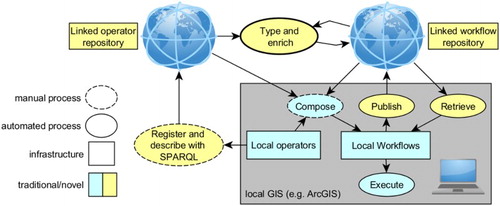
In this article, we focus on how to add the necessary semantic information to a ‘raw’ workflow produced by a GIS in order to make its elements easily publishable and reusable over the web (see Figure 1). We do not focus on the exploitation of web resources for general workflow construction or execution, for which satisfactory tools already exist (see Section 2). Our central tenet in this article is that implicit information contained in GIS operations can be used to propagate types through a workflow, and thus to automate workflow typing, that is, the assignment of types to workflow elements. In this sense, we see geoprocessing workflows in themselves as a valuable and yet neglected source of data semantics (Scheider et al. 2016), which can be exploited to automate the publication of GIS methods, supporting workflow reuse.

Considering a familiar example, the fact that a raster file was generated, for example, by a least-cost path operation³ is an essential piece of information that unveils the resulting raster file represents a path and not, for instance, a temperature field. This is crucial: In contrast to a temperature field, a path cannot be spatially interpolated (Stasch et al. 2014). However, this information is usually kept in the mind of the analyst or, at most, described in vague natural language. In order to reuse the workflow to generate similar paths in different regions, other analysts would need to read the documentation, study the workflow structure closely, and substitute appropriate data sources based on the types of input. Moreover, knowledge about types of results is also crucial for reuse, for example, to appropriately use the resulting path in a network analysis (Geertman, de Jong, and Wessels 2003). Our main argument is that the implicit knowledge contained in a geoprocessing workflow can be used to add this essential piece of semantics to data in a partially automated way, and thus adding the central element of enrichment to a future architecture for workflow management (Figure 1).

To capture the types of origin and results in workflows, we propose a method for semantically typing geoprocessing workflows on the level of their operations and datasets. The method explicitly records the semantics of workflows using linked data as infrastructure. Following the linked data paradigm (Kuhn, Kauppinen, and Janowicz 2014), workflow resources are described in resource description framework (RDF), making them shareable on the web. We harness the core concepts of spatial information (Kuhn 2012), some ideas from typed functional programming, and previous work on GIS typing and spatio-temporal information generation (Scheider et al. 2016; Scheider and Tomko 2016). From a technical perspective, we apply SPARQL⁴ rules for well-known GIS operations and use OWL2 RL inferences⁵ to enrich the workflow with semantic types. These types are based on a suite of GIS ontologies in OWL2.⁶ The formal ontologies are available online (Section 3), and all sources implemented in Python are fully available on GitHub (http://github.com/simonscheider/SemGeoWorkflows).

Semantic typing enables new kinds of interaction with and exploration of workflows and related resources. Borrowing the term from Gangemi and Presutti (2009), analysts can now ask new kinds of competency questions, defined as queries that they want to pose to a workflow repository to solve a given analysis task. In this article, we show how analysts can:

Select: Select workflows based on their types of inputs and outputs; Retrieve datasets compatible with a given operation.

Adapt: Substitute inputs of workflows with other datasets; Combine compatible workflows into chains.

Recommend: Show possible operations to continue the workflow; Recommend datasets compatible with a given operation; Recommend operations compatible with a given dataset.

The remainder of this paper is organized as follows. In Section 2, we discuss related work. Section 3 introduces our approach and its ontological foundations, while Section 4 outlines the type enrichment rules and the propagation mechanism. In Section 5, we describe two moderately complex, real-world ArcGIS workflows with linked data, and Section 6 shows how our automatic enrichments support the set of competency questions. Finally, we draw conclusions and suggest directions for future work in Section 7.

2. Related work

The complexity of building and managing scientific workflows has long been recognized, but progress has been modest. In their influential discussion on scientific workflows, Gil et al. (2007) noted that usable support tools to develop and document workflows are key needs of the scientific community. To mitigate the inevitable problem of heterogeneity of computational environments, tools, datasets, and procedures, ‘scientists should be encouraged to bring workflow representations to their practices and share the descriptions of their scientific analyses and computations in ways that are as formal and as explicit as possible’ (p. 26). However, current approaches in workflow management software focus on workflow construction and execution, and not on their modular integration and sharing.⁷ Notably, semantic systems such as Pegasus and Wings⁸ help practitioners assemble complex computational procedures from smaller parts, and thus to control, reproduce, and scale up the computational process, but without explicit support for spatial operations.

2.1. Re-usability

Current approaches to reproducibility and re-usability of research methods (which often include geoprocessing workflows) rely on the idea of re-computation (Rey 2009; Müller, Bernard, and Kadner 2013; Singleton, Spielman, and Brunsdon 2016). Reproducing and reusing spatial analysis methods, however, goes considerably beyond re-computing or replicating workflows (Drummond 2009). In fact, workflow models are usually dependent on a particular software and data environment, and thus cannot cope well with unavailable data, nor do they allow easy substitution of parts of a workflow with equivalent data or methods. Research data can be unavailable for various reasons, including privacy and licensing restrictions. Once cast into software, methods become dependent on a particular context, making methodological decisions hidden in the parameters of that particular software environment (Hinsen 2014).

2.2. Web service semantics

One way out of this dilemma consists of increasing the intelligence of workflow specifications, instead of simply building new applications to manage them (Janowicz et al. 2015). In this direction, in the early 2000s, Visser et al. (2002) discussed the potential of formal semantics encoded in ontologies to re-structure GIS into inter-operable pieces. Similarly, many researchers noted that matching inputs and outputs of geoprocessing Web services with keywords is insufficient and should be substituted with formal semantics for automation of workflow construction (Lemmens et al. 2006; Lutz 2007; Yue et al. 2007; Fitzner, Hoffmann, and Klien 2011). As a remedy, Lutz designed a method based on function subtyping to assess for example if two geoprocessing workflows can be chained (i.e. the output of the first one is compatible with the input of the second one), based on Description Logics (DL) and First-Order Logic (FOL). Fitzner, Hoffmann, and Klien (2011) demonstrated how to efficiently match services with requests based on Datalog rules and GIS ontologies. Despite their conceptual clarity, these approaches have not found yet wide adoption (Hofer 2015). As a matter of fact, their service orientation makes them dependent on a certain software environment in the form of web services.

2.3. Linked data workflows

More recently, workflow models based on the linked data paradigm have emerged as a way to abstract from particular computational contexts, thus making provenance sources explicit and shareable on the web (Moreau and Groth 2013; Belhajjame et al. 2015).⁹ These vocabularies have lately been integrated with standard GIS data models and processes (Closa et al. 2017). However, while current models describe specific provenance contexts (i.e. what agent and what tool were involved in the computation of what result at what time), they often lack a way to generalize over types of input and output data and to highlight their specific roles in the generation process (Daga et al. 2014; Alper et al. 2015). In particular, they lack spatial concepts, such as networks, fields, and objects (Kuhn 2012), and an account of the inherent logic of GIS operations as analytic tools (Anselin, Rey, and Li 2014).

Brauner (2015) recently suggested an approach to annotating geo-operators with linked data to make them comparable across applications. In his survey of this area, Müller (2015) confirms that a mechanism for the semantic description of functionality is still missing. However, none of these authors specifically addressed the problem of how to semantically enrich geoprocessing workflows. To bring workflows out of the current silos, we argue that researchers should focus precisely on the semantic abstraction of workflows from local environments, such as ArcGIS, QGIS, or R, and less on developing semantic service infrastructures. This would allow analysts to share their methods on the web, without having to migrate from their favorite tools and environments.

2.4. Semantic typing

Data types generally increase the transparency and clarity of a program, helping developers express expected inputs and outputs of computational resources, for example specifying whether a function input is a string, an integer, a raster dataset, or another function. The success of types in object-oriented programming lies in information hiding, which is a way of abstracting from implementation details (Guttag and Horning 1978). More specifically, type constraints allow for modularity, that is, they guide the choice of a function, and open slots can be filled with particular data of a corresponding type to obtain a desired result. A second advantage is constructivity, the ability to construct a variety of types by combining primitive ones. And a third advantage is type inference, that is, the possibility to use inference rules to automatically guess the types of output and input when applying an operation. In practice, this greatly reduces a programmer's efforts of documenting code.

Existing languages, however, tend to focus on the construction and execution of code, not on sharing methods or procedures. The strength of Semantic Web technology and linked data, by contrast, lies precisely in the ability to share types on the web and to construct and infer types in a much more flexible, distributed way (Kuhn, Kauppinen, and Janowicz 2014). Classes and relations that are used to type and link resources can be used in tractable inferences. For instance, where programming languages tend to require unique types to remain tractable, a given resource can be typed with an arbitrary number of OWL classes. While data types in programming focus on technical interoperability, classes in OWL can capture specific semantic content on the level of the application domain. This was a driver behind the development of ontology-based web service descriptions, such as WSMO.¹⁰ In practice, however, such approaches have been seldom combined with GIS-specific concepts that go beyond basic data formats (Fitzner, Hoffmann, and Klien 2011). Furthermore, WSMO targets web services, not workflows. For all these reasons, we propose a typing scheme based on linked data technology, tailored to geoprocessing workflows. As we will show below, our scheme is modular, to some extent also constructive, and it allows for type inference.

3. A linked data typing scheme for geoprocessing workflows

Geo-data generated in workflows obtains an implicit semantics as a consequence of applying GIS operations with certain concepts in mind. Our linked data typing scheme is designed to capture this semantics. To this end, we first introduce types for spatio-temporal concepts and for GIS. Subsequently, we introduce a linked workflow vocabulary that can be used to add implicit semantic structures based on provenance.

3.1. Types for spatio-temporal concepts

When designing workflows, spatial analysts commonly think of data at a more abstract level, using meaningful concepts, such as objects, fields, and networks. GIS data types are not sufficient for this purpose. As argued in previous work, we can better capture the semantics of spatial data in terms of spatio-temporal (core) concepts, which are orthogonal to GIS data types (Kuhn 2012; Scheider et al. 2016).

The most fundamental kinds of concepts are references for space, time, quality, and object, summarized in Table 1. These are values that refer to observable or measurable phenomena, such as time moments, space regions, and qualities that are referenced by measurement scales. For example, coordinate pairs of a statistical region's boundary refer to locations on the Earth's surface, and its attribute number might refer to the population counted in that area. Among the references, we also include objects – discrete entities such as buildings, and cars, including events such as hurricanes. Note our distinction of objects from qualities, such as a temperature or the number of objects in a community (Stasch et al. 2014). Additionally, we also consider collections of things, such as object clusters.

Table 1. Types of spatio-temporal references.

Reference type	Example of reference system
Space	WGS84
Time	UTC
Object	National address system (for buildings)
Quality	Size, weight, temperature

The second kind of fundamental spatial concepts are observation procedures, represented in terms of functions that map from reference domains to other reference domains, as summarized in Table 2 and described in detail in previous work (Scheider et al. 2016). For example, fields (i.e. measures of spatially continuous phenomena) can be defined as functions from space and time to qualities. Spatial fields (SField) can be seen as functions from space to quality values, object time series (TSeries) as functions from discrete object identifiers and time to quality, and trajectories as functions from time to space. Note that these functions are not datasets, but rather stand for the potential to measure or observe references.

Table 2. Types of functional concepts.

Functions	Derived functions
Field (Time Space Quality)	SField (Space Quality)
Objects (Object Time Quality, Space)	TSeries (Time Quality)
Objects (Object Time Quality, Space)	Trajectory (Time Space)

3.2. GIS types

GIS adds more specific references and data types to this scheme. For example, in GIS, certain relatively defined references are common, such as Neighborhood and Path objects (see Table 3). A neighborhood object depends on a host of which it is the neighborhood – an example is a spatial buffer (Burrough et al. 2015). And a path object is the basic element of a network dataset, representing a possible move from some start object to an end object, for example, a road segment leading from intersection to intersection.

Table 3. GIS-specific types of references.

Reference class	Example	Super concept
Path	Road segment	Object
Neighborhood	Buffer region	Object
Cost	Environmental costs	Quality
Density	Density of objects	RelQ
Distance	Cost distance, Euclidean distance	RelQ
QQuality	Map algebra sum	RelQ

As shown in Table 3, qualities in GIS can be complex. Beside unary qualities like Cost, there exist relational qualities (RelQ) whose values depend on other datasets (Probst 2008). One example for such a quality is a Density, which derives from a set of objects. Another one is a Distance quality to a set of objects. A special kind of distance is a CostDistance, which corresponds to the shortest distance between a source and a sink on a cost surface. Another special relational quality is called QQuality, a quality derived from another quality of another dataset. Whenever we compute a sum in map algebra (Tomlin 1990), we generate a raster quality from other raster qualities, for example comparing luminosity from two different times. To capture such provenance dependencies, we define the relation of, stating that a density is a density of a particular set of objects, or a distance to a particular set of objects (cf. Figure 3).

GIS datasets are discrete representations of spatial concepts (Table 4). This idea was introduced as a linked data pattern¹¹ to handle datasets and references in the context of spatial analysis (Scheider and Tomko 2016). Datasets, such as GIS layers, have data items as their elements, and these items have spatial and non-spatial references, just as rows in a GIS table have geometry and attribute values (Figure 2).

Figure 2. Distinction between data items, supports, and measures.

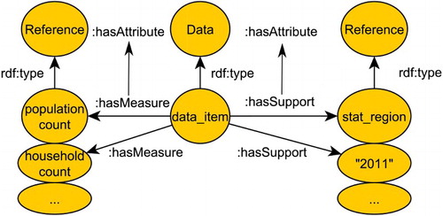
Table 4. GIS data types.

GIS data type	Support	Measure
Raster	Region	Quality
ObjectDataset	Object	Quality, Region/Line/Point
VectorDataset	Region/Line/Point	Quality
Track	Time	Point
Network	Path	Quality

In contrast to a pure table schema, we draw a conceptual distinction between references based on the role they play in observation. A measure denotes an observed reference of a data item, whereas a support denotes the context of this observation that can be used to compare measures. Supports and measures are both attributes of a data item (see Figure 2).¹² For example, a statistical data record may have a population count quality as measure, and a spatial region and a time as support, meaning that the measure was observed for this region and this time (Figure 2). In GIS, raster datasets measure qualities over regular squares, while vector datasets measure qualities over points, lines, and arbitrary regions. Tracks, by contrast, measure the locations of some moving object over different times. Object datasets have object identifiers as supports, and a Network has paths as supports (see Table 4).

Another ontology pattern is used to define these GIS-specific data types.¹³ Both patterns combined are illustrated in Figure 3. Each black arrow stands for a relation between instances of some class, where classes are denoted by ellipses or round boxes, the latter standing for classes of functions. The relation are in the diagram means that the first class is a subclass of the second.

Figure 3. Concepts for typing geoprocessing workflows. Provenance relations are denoted by the property of. Rectangles: function classes.

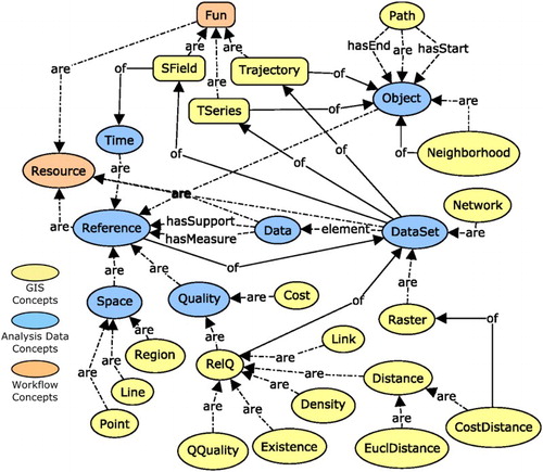
It is important to distinguish between data types and spatial concepts because concepts can be represented by almost any arbitrary data type, but only the concepts are relevant for analysis. For example, depending on how it was generated, a raster dataset can indirectly represent both objects and fields, and this distinction can only be made based on its provenance.

More precisely, if we measure temperature quality values at points in space, then, implicitly, we sample a spatial field (SField) in the environment. The type of this data may therefore be called Points of SField, and needs to be distinguished from a point data file representing the location of objects (Points of Objects), which was generated by observing objects in the environment (see Figure 4). While a Points of SField can be interpolated, Points of Objects cannot (Stasch et al. 2014). Furthermore, if we interpolate our point sample file to a raster, then the resulting raster represents the spatial variations of the underlying field in a discrete form (Raster of SField). In contrast, if we convert a set of objects represented as vectors to a raster, we obtain an Existence Raster (a raster of the existence of some objects) (See Figure 4). This raster file represents nothing but the presence of discrete objects, and thus cannot be interpolated either.

Figure 4. Provenance graph of GIS types derived from the concepts ‘field’ and ‘object’. Black arrows link concepts to predecessors in the geoprocessing chain. Concepts indirectly represented as data are denoted by dotted boxes (e.g. fields are indirectly represented by rasters).

In summary, whenever we apply a GIS operation, we generate new data, but we also, indirectly, determine its semantics in terms of spatial concepts (cf. Figure 4). For this reason, we must keep track of these concepts via provenance. The vocabulary discussed in the following section captures some of the necessary semantic provenance relations inside workflows.

3.3. Typing workflows as linked data graphs with implicit semantic structures

In order to type workflows with provenance relations and concepts, we propose to represent them in terms of an OWL pattern,¹⁴ as illustrated in Figure 5. Workflows must be treated both as individual entities, recording their creation context, and also as graphs linked with these entities, capturing the workflow structure. Furthermore, functional dependencies between inputs and outputs need to be included (Fitzner, Hoffmann, and Klien 2011), as well as implicit concepts that exist in the background (Scheider et al. 2016).

Figure 5. Linked data pattern (classes and properties) for modeling workflows. Workflows are linked to their subgraphs via reified statements. Operations are functions applied to inputs and producing outputs, resources are used to build a workflow (may also be functions). The of relation links resources to their origins.

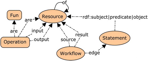
In order to achieve these objectives, we link workflow individuals to workflow edges via the wf:edge property. Edges are reified RDF statements, denoting workflow steps, of the form:

[some wf:Operation] [wf:input|wf:output] [some wf:Resource].

To distinguish different types of input, we can introduce sub-properties of wf:input. For example, in the gis vocabulary, we indicate input parameters as gis:inputdata. Later, we will also use tool specific input properties in Section 4.2. The reification¹⁵ of these statements is implemented using rdf:subject, rdf:predicate, and rdf:object triples that connect the three elements of a statement to the workflow edge. For example, the workflow in Figure 6 consists of two such statements for input and output. Thus, it is possible to query workflow individuals and their graphs at the same time, and to store the information about inputs and outputs of a workflow through the properties wf:source and wf:result.

Figure 6. Example of usage of the workflow pattern wf to add explicit and implicit (dotted) semantic structures between inputs and outputs in a geoprocessing workflow for point interpolation.

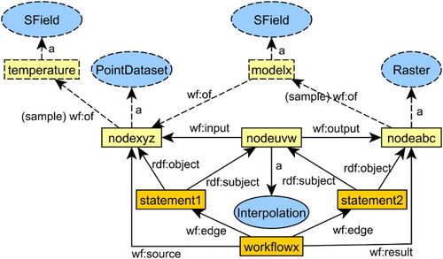
The nodes of the edges of the workflow graph, representing resources and operations, can now be typed using OWL classes. Furthermore, implicit semantic structures can be added. For example, in Figure 6, interpolation requires an implicit underlying spatial field (in this case of temperature) from which the workflow source, a point dataset, was sampled. Although this field is an entity outside of the workflow and thus not represented in terms of data, it can be made explicit with linked data by introducing a blank node.¹⁶ Furthermore, there are also implicit semantic structures hidden in the operation. For instance, interpolation requires an interpolation model, a spatial field (a function from space to a quality) estimated by the point data set.

By adding implicit semantic structures based on the relation wf:of, we now know that the result of the workflow is not simply a raster dataset, but it is of the complex type Raster (sample) of an SField of a Point data set (sample) of an SField, information that simply gets lost in current tools. In order to distinguish different types of provenance relations, we can further introduce sub-properties for wf:of. In this article, we use only a single sub-property wf:ofprop, which denotes the provenance relation between measured qualities (QQuality). Table 5 gives an overview of the three ontologies that we use in workflow typing.

Table 5. Vocabularies used in this article.

Vocabulary	Prefix	URI
Workflow	wf:	http://geographicknowledge.de/vocab/Workflow.rdf#
GISConcepts	gis:	http://geographicknowledge.de/vocab/GISConcepts.rdf#
AnalysisData	ada:	http://geographicknowledge.de/vocab/AnalysisData.rdf#

4. Type enrichment based on GIS operations

In this section, we introduce rules for the semantic enrichment of workflows based on well-known GIS operations, expressed in SPARQL language.¹⁷ We start with algorithms and enrichments based on single tools, and then proceed to type propagation rules over whole workflows.

4.1. Tool-based semantic enrichment and avoidance of redundancy

Whenever analysts execute a GIS operation in a workflow, they make certain assumptions about the meaning of its inputs and output. We take the view that these assumptions are made independently for single tools or a class of tools, based on the idea that classes of geoprocessing tools have a common purpose and treat spatial concepts behind the data they produce in a comparable manner. Classes of tools can be built based on OWL subclass relationships, and enrichments can be made with a corresponding semantic signature for each type of tool.¹⁸

The typing of input and output in a workflow is done by applying rules expressed as SPARQL Update statements.¹⁹ The types of tools are in the condition of the statement, and the types of inputs and outputs are in the statement's head. However, in order to make our enrichment method reliable, we have to care about consistency in typing and about linking implicit semantic structures across a potentially complex workflow. If we just naively added implicit semantic structures to inputs and outputs of an operation, we would generate many unconnected and redundant nodes. For example, the dataset represented by node 3 in Figure 7 may receive a similar semantic structure from operations at node 2 as output, as well as node 4 as input, and it would remain unclear how these structures relate to each other.

Figure 7. Backtracking from sources to results to enrich a workflow. For each operation, we first type inputs (if not already present), then outputs, and then link outputs to inputs, and then proceed to the next operation.

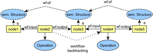
In order to prevent the generation of such unconnected structures, we perform the typing in a specific order, starting from inputs to outputs, from the sources of a workflow to its result. This way, newly introduced structures on an operation's output can be reused as input on the next operation. This can be achieved by searching through a workflow graph with a Depth-First Search (DFS), starting from its result, and then backtracking on the operations. As a result, blank nodes introduced as an operation's output can be linked back to its predecessor's output.

Since workflows can be viewed as trees with a result as root and branches for distinct inputs, we have to consider branching inputs of the same type. Also in this case, naively generating output structures for an input structure can cause redundancy, because update statements need to run once for each input branch. We prevent this by separating the introduction of blank nodes for inputs and outputs from linking them, generating different rules for these three aspects of an operation. Second, we introduce blank nodes in a conservative way, simply by checking whether they already exist.

Algorithm 1 illustrates the search procedure that takes into account these problems. The procedure searches through operations of a workflow, breaking down the problem into steps of introduction and linking of semantic structures for inputs and outputs of a given operation. After this step, Algorithm 2 illustrates the procedure to apply sequentially the input, output, and link rules to the workflows.²⁰

4.2. Enrichment rules for classes of GIS operations

To implement our approach, it is necessary to design typing rules, expressed as SPARQL statements, for a selection of tool categories, ranging from format conversions, to map algebra and topological operations, and least-cost path computations. The choice of these operations was driven by the two example workflows, which will be described in detail in Section 5. However, the selection could be expanded to a full-blown GIS operator web repository. To show the practical applicability of the method to existing systems, we refer to the implementation of these operations in ArcGIS, using the ESRI terminology. For the sake of brevity, we explain here only three exemplary operations. Others are explained in the Supplementary Material as they appear in our workflow examples.²¹

Raster to vector conversions ²² are a ubiquitous and simple GIS operation, but rather complex from a semantic viewpoint. This is because the input raster is required to be an existence raster of some single object, which is turned into either a discrete point, a line, or a region in the output. Such conversion ignores raster measures, taking them as existence qualities of some object, and therefore rasters of some field are not a meaningful input to this operation. The challenge lies in the integration of the outputs with the input raster's existence quality. Note that input (Listing 1) and output rules (Listing 2) introduce blank nodes for measures and objects, which are then linked in Listing 3.

The following rules express this semantics: (a) The input data set is an existence raster of objects; (b) these objects are supports of the output data set.

Listing 1. Raster to Line SPARQL input rule

Listing 2. Raster to Line SPARQL output rule

Listing 3. Raster to Line SPARQL link rule

Note that we use the filter not exists statement in input and output rules to check whether semantic structures already exist or not. Because input and output rules only introduce the blank nodes necessary for linking, we omit them in the following listings.

The cost distance tool takes a cost surface raster and a sink raster, and then generates a raster measuring the link (i.e. the successor cell) of the least-cost path toward the sink.²³ The sink raster is an existence raster of objects, while the surface raster represents a cost field. Both assumptions are made explicit, and we also add provenance relations between output data and cost surface measure with respect to the sink dataset (Listing 4).

Listing 4. Cost Distance SPARQL link rule

The cost path tool takes a link raster to a sink (generated by the cost distance tool) and a source raster, and generates a raster that represents the least-cost path from source to sink.²⁴ As above in the case of the sink, the source raster represents the existence of source objects, while the output raster represents the existence of a new kind of object, namely a path (Listing 5).

Listing 5. Cost Path SPARQL link rule

Other operator rules can be found in the Supplementary Material.

4.3. Type propagation rules

Further rules can be added that integrate types over more than one operation in the workflow. Such rules can use property paths in SPARQL in order to express queries over workflows of arbitrary length.²⁵ Property paths are conceptually similar to regular expressions, widely used in natural language processing and data mining. For example, we define a rule that propagates provenance links (wf:of) over paths (using +) of QQuality links (gis:prop, inverted by ^) of arbitrary length, such that the resulting quality has the same provenance relations. Thus, it becomes possible to preserve provenance information whenever a property is derived from another one, such as in local map algebra or in conversions. In the following rule, a is the start quality of the path (assured by the filter statement), and b is the end quality that is enriched with provenance statements (Listing 6).

Listing 6. QQuality SPARQL propagation rule

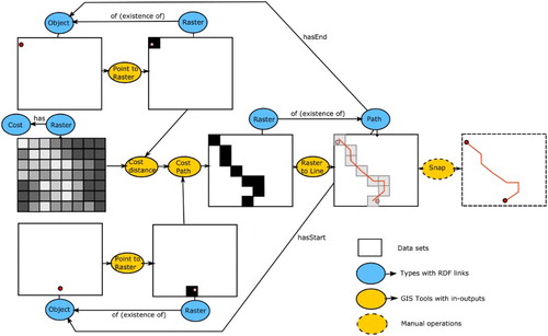
Another rule connects start and end object vector datasets to a path object by integrating cost distance and cost path operation inputs and output, taking into account implicit semantic structures added by conversion operations (Listing 7, see Figure 8).

Figure 8. Schematic map illustration of least-cost path integration. Arrows between RDF types stand for links between their instances.

Listing 7. Path integration SPARQL propagation rule

A last rule generates the transitive closure of part-of statements through a workflow in order to find out about the sources of spatial aggregations (Listing 8). As usual, a filter is used to avoid redundancies.

Listing 8. Part-of transitivity SPARQL propagation rule

5. Semantic enrichment of ArcGIS workflows

In this section, we describe two well-known and practically relevant workflow scenarios designed with the industry standard ESRI's ArcGIS ModelBuilder (Allen 2011). We show how to turn them into pure untyped linked data, providing a basis for the semantic enrichment that will be described in Section 6.

5.1. Workflow #1: Analysis of night lights in China

In an econometric study, the analyst wants to estimate the growth in China spatially – at the local level – and temporally – at different times – using night light as a proxy of economic activity (Lowe 2014).²⁶ This research question is translated into a geoprocessing workflow that operates on the following input datasets: satellite imagery about nocturnal luminosity (raster), a map of gas flares (vector), country boundaries of the whole world (vector), and road network in China (vector). While not overly complex, this workflow is a realistic example of geoprocessing on real data. The workflow, as described by Vahedi, Kuhn, and Ballatore (2016), consists of the following steps:

1. Remove gas flares from China region.

2. Calculate a buffer around train stations.

3. Intersect China raster without gas flares and buffered train stations.

4. Convert the resulting vector data to raster.

5. Mask luminosity rasters for times and with the resulting raster.

6. Calculate zonal mean, using administrative units as zones for and .

7. For each zone, calculate the change between and .

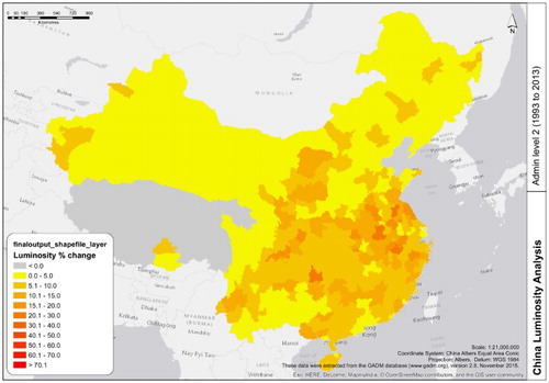
Figure 9 shows an implementation of this geoprocessing workflow, developed with ArcGIS ModelBuilder. The diagram shows input datasets, GI operations, and output datasets, leading to the final dataset (Luminosity_change). For the sake of clarity, Figure 10 represents an example of the change in luminosity from 1993 to 2013 across China, grouped by administrative units.

Figure 9. Workflow #1: ModelBuilder workflow to calculate the change in night lights in China. The blue ovals are input datasets, yellow rectangles indicate operations, and the green ovals are output datasets.

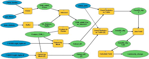
Figure 10. Workflow #1: Variation in average nocturnal luminosity over China from 1993 to 2013. Courtesy of Andy Bartle (Birkbeck, University of London).

To enable our semantic typing approach, the workflow must be described according to the workflow ontology (wf). Listing 9 shows a translation of RDF generated based on the workflow in Figure 9. The node :wf1 is the workflow, linked to a number of data sources, and to a result. Each node (wf1_x) corresponds to an operation, represented as yellow rectangles in the model, and is typed according to the GIS operation performed (e.g. gis:Erase), with inputs and outputs.

Note that this compact RDF annotation does not require any semantic typing of the datasets, which will be generated automatically by the enrichment mechanism, propagating the types across the nodes from the inputs to the outputs in a deterministic process. In this sense, a clear advantage from the user's perspective is the limited explicit input, yet resulting in a rich and powerful description of the workflows and their associated resources.

Listing 9. Semantic description of Workow #1

5.2. Workflow #2: Planning of a new road with LCP

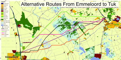
The following workflow is taken from an advanced GIS course given at Utrecht University by the department of Human Geography and Spatial Planning.²⁷ It was designed by Tom de Jong (Geertman, de Jong, and Wessels 2003) and is based on a realistic planning scenario in which the province of Nordland in the Netherlands intends to improve the accessibility of its highway network by building a new highway link between existing entries and exits. Students need to suggest possible links (Figure 12) based on a multi-criteria analysis workflow in GIS, from which we chose only the first steps (least-cost path analysis), as shown in Figure 11. The following input datasets are used: a highway exit and entry point (chosen from a digital road network), a landuse dataset (vector), a dataset of built areas (vector), a dataset of nature habitats (vector).

Figure 11. Workflow #2: ModelBuilder workflow of planning a new highway (myroute) connecting two highway exits (endraster, beginraster) based on avoiding built environment, nature areas, and other landuse classes. The latter objects enter the model in terms of a cost surface on which a least-cost path is computed. Blue ellipses denote root data sets, green ones intermediate data, and yellow boxes denote function applications.

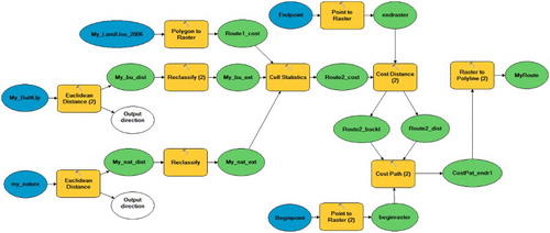
Figure 12. A map of different road alternatives generated based on the workflow of Figure 11. Courtesy of Tobias Dobbe, Jorn Neppelenbroek, Thomas Kuijpers and Jip Zinsmeister.

1. Compute a raster of Euclidean distances to build up areas and nature habitats with identical extent and cell area

2. Reclassify distances to generate a cost criterion (output of 1)

3. Convert landuse vector dataset into a raster with identical extent and cell area by a polygon to raster conversion

4. Use local map algebra to combine criteria (outputs of 2 and 3) into a cost surface based on a weighted sum

5. Convert begin and end point objects (highway exits) of a road network to a raster

6. Compute the least-cost (distance +) path between begin and end point rasters (output of 5) using the cost surface (output of 4)

7. Convert least-cost path (output of 6) raster into a polyline

Since it follows a similar structure to Workflow #1, we omit the RDF listing for this workflow.²⁸ Both these workflows are enriched in the next section.

6. Evaluation of semantic enrichments on example workflows

This section shows how we perform the type enrichment, using ordinary RDFS and OWL RL inferences (Grosof et al. 2003), and how this can help answer competency questions about workflows and data, as posed in the introduction. In what follows, we distinguish resources of the two workflows based on the prefixes cnl (Workflow #1, China lights) and lcp (Workflow #2, least-cost path).

6.1. Running inferences on the workflows

The enrichment and propagation process loads the workflows, the relevant ontologies, and then proceeds to run RDFS and OWL RL inferences. Subsequently, the enrichment and propagation rules are applied. To show a full iteration of the process, when running on workflow lcp, the script grows an RDF graph in the following steps:

1. Loading workflow (32 triples);

2. Loading ontologies (576 triples);

3. Running OWL RL inferences (2205 triples);

4. Running tool-based type enrichments (2292 triples);

5. Running type propagations (2297 triples);

6. Running OWL RL inferences again (2912 triples).

The execution of the process above took 12 seconds on an ordinary PC,²⁹ and the majority of the time is taken up by the OWL RL inferences.³⁰ Running the same procedure only with RDFS inferences took only 3 seconds, resulting still in slightly more than half of the inferences (1658 triples). Note that even though OWL inferences are not particularly efficient, our procedure scales well with the number of workflows, since only type enrichments depend on this number, and they are computationally inexpensive, while inferences can be run independently over all triples. Hence, we claim that the process is reasonably fast to be executed on ordinary machines and current triple stores, even in realistic scenarios with large repositories of interconnected workflows.

6.2. Competency question 1: Select data and workflows

Thanks to the semantic enrichments and propagations, we can now perform a more targeted selection of datasets, data items, and data references used in workflows, including provenance information. For example, we can select datasets with path objects, together with the datasets containing their start and end objects (Listing 10). As shown in Table 6, this query returns the respective input and output data sets that are origins of the path object generated in the Least-Cost Path workflow (namespace lcp:). Note that the long hash in the path object column is the identifier of a blank node.

Table 6. Result of the query in Listing 10. Path datasets with start and end objects.

Dataset	Path object	Start dataset	End Dataset
lcp:MyRoute	N5bbadf73ba1745	lcp:beginpoint	lcp:endpoint

Listing 10. Get paths together with start and end objects

Similarly, we can obtain all datasets that are spatial aggregations of rasters, together with their aggregation windows (regions of aggregation) and the source raster (Listing 11). Table 7 shows that the result of the china lights workflow was in fact aggregated from the luminosity raster over the spatial windows of Chinese border and the neighborhoods of train stations, information that can be used to interpret and constrain the further usage of this dataset.

Table 7. Result of the query in Listing 11. Aggregated datasets and the input regions.

Aggregated dataset	Source	Window
cnl:Luminosity_change	cnl:F101993_night_lights	cnl:CHN_adm0_Erase_Intersect
cnl:Luminosity_change	cnl:F101993_night_lights	cnl:China_border
cnl:Luminosity_change	cnl:F101993_night_lights	cnl:Chn_atm0_erase
cnl:Luminosity_change	cnl:F101993_night_lights	cnl:Ch_Stations_Buffer

Listing 11. Get windows and sources of spatial aggregations

More generally, using OWL RL inferences to capture data types defined in the GISConcepts ontology, we can now search for datasets based on very specific types and provenance relations (Listing 12). The results in Table 8 contain all datasets of the lcp workflow, along with their inferred dataset types and types of provenances (related by wf:of).

Table 8. Result of the query in Listing 12. Datasets, their types and provenance types.

Dataset	Type	of Type	of Type
lcp:Route2_cost	gis:Raster	gis:SField	gis:ObjectDataSet
lcp:My_LandUse_2006	gis:RegionDataSet	gis:SField
lcp:my_BuiltUp	gis:ObjectDataSet
lcp:CostPat_Begi1	gis:Raster	ada:Object
lcp:Beginraster	gis:Raster	gis:PointDataSet	ada:Object
lcp:Route1_cost	gis:Raster	gis:SField
lcp:My_bu_dist	gis:Raster	gis:SField	gis:ObjectDataSet
lcp:beginpoint	gis:PointDataSet
lcp:endpoint	gis:PointDataSet
lcp:Route2_backl	gis:Raster	gis:RegionDataSet	gis:Raster
lcp:MyRoute	gis:ObjectDataSet
lcp:MyRoute	gis:Network
lcp:MyRoute	gis:LineDataSet
lcp:my_bu_ext	gis:Raster	gis:SField	gis:ObjectDataSet
lcp:endraster	gis:Raster	ada:Object	gis:PointDataSet

Listing 12. Get datasets their types and provenance

Note that the data nodes in the workflow now have types inferred from the operation and not specified in the initial workflow descriptions, such as gis:ObjectDataSet, gis:PointDataSet, gis:LineDataSet, gis:RegionDataSet and gis:Network. For example, the workflow result lcp:MyRoute is not only an object data set, but is also a line data set, as well as a network. Furthermore, we can now distinguish datasets according to their provenance. For example, lcp:My_LandUse_2006 is a region data set that represents some categorical spatial field (namely landuse), while lcp:Beginraster is a raster that represents an object contained in a point data set. These distinctions can be crucial in helping a GIS analyst use the dataset according to its intended meaning.

Table 9. Result of the query in Listing 13. Select workflows based on their result types.

Workflow	Result	Type of Dataset
lcp:wf2	lcp:MyRoute	gis:ObjectDataSet
lcp:wf2	lcp:MyRoute	gis:LineDataSet
lcp:wf2	lcp:MyRoute	gis:Network

Using the same logic, we can query for workflows based on which types of results they produce. For example, we may be interested in all workflows that generate networks (Listing 13). This competency question can be used to chain workflows, making sure that their inputs and outputs are compatible types.

Listing 13. Get workows by result type

6.3. Competency question 2: Adapt input data in workflows

Given an operation in a workflow, a common task consists of finding possible new input datasets that make sense in the context. For this purpose, we can query for datasets that have the implicit semantic structure of our input enrichment rules for a given operation, including classes and properties. In the two example workflows, this approach obtains meaningful suggestions of data from other workflow nodes, excluding non-meaningful matches that would occur in naive data type matching, as illustrated below.

Here is an example of a query for the operation gis:PolygontoRaster, which restricts inputs both by requiring the existence of structures as well as their absence (no raster allowed). Such negative type restrictions become necessary since we are considering non-unique types (Listing 14).

Listing 14. Get matching input datasets for a workow operation

The result lists workflow operations together with meaningful input dataset matches (Table 10). As is possible to notice, we obtain a field-based region dataset (lcp:My_LandUse_2006) as input for gis:PolygontoRaster, while region data sets that represent objects are excluded. We get other object-related raster data (e.g. other road objects) as source input (input 2) for gis:CostPath, while its link input is restricted to those raster datasets which have link qualities (in our case, only lcp:Route2_backl).

Table 10. Result of query in Listing 14. Find possible inputs for operations in a workflow.

Operation	Type	Matching input 1	Matching input 2
lcp:0	gis:PolygontoRaster	lcp:My_LandUse_2006
lcp:7	gis:CostPath	lcp:Route2_backl	lcp:endraster
lcp:7	gis:CostPath	lcp:Route2_backl	lcp:CostPat_Begi1
lcp:5	gis:CostDistance	lcp:Beginraster	lcp:Route1_cost
lcp:5	gis:CostDistance	lcp:Beginraster	lcp:My_bu_dist
lcp:5	gis:CostDistance	lcp:Beginraster	lcp:my_bu_ext
lcp:5	is:CostDistance	lcp:CostPat_Begi1	lcp:Route1_cost
lcp:5	gis:CostDistance	lcp:CostPat_Begi1	lcp:My_bu_dist
lcp:8	gis:toLine	lcp:endraster
lcp:8	gis:toLine	lcp:Beginraster
lcp:8	gis:toLine	lcp:CostPat_Begi1
lcp:4	gis:PointtoRaster	lcp:beginpoint
lcp:6	gis:PointtoRaster	lcp:endpoint
lcp:3	gis:LocalMapAlgebra	lcp:Route2_cost
lcp:3	gis:LocalMapAlgebra	lcp:My_bu_dist
lcp:2	gis:LocalMapAlgebra	lcp:Route1_cost
lcp:2	gis:LocalMapAlgebra	lcp:Route2_cost
lcp:2	gis:LocalMapAlgebra	lcp:my_bu_ext

The gis:CostDistance operation is more variable in taking field related raster data as cost surface input (input 2). For example, it would admit also rasters that represent distance fields (lcp:My_bu_dist) or the landuse cost raster (lcp:Route1_cost), but object-based rasters are excluded. However, this operation may take other object-related rasters as its sink input, such as lcp:CostPat_Begi1 or lcp:Beginraster, similar to the conversion operation gis:toLine. gis:PointtoRaster would allow other point data sets. gis:LocalMapAlgebra allows alternative field-based rasters or object-based rasters as input, but excludes rasters with other qualities as measures, such as link qualities. While we did not find evidence of non-meaningful suggestions in this evaluation, a systematic evaluation of whether such inputs are useful for a given task goes beyond the scope of this paper.

6.4. Competency question 3: Recommend tools

Given the type enrichments of datasets, we can use an operation's type restriction to suggest compatible tools. This competency query is solved in an equivalent way, but reverting the direction: We search over the input restrictions of each operation's enrichment rule, and recommend those operation types that match a given dataset (Listing 15). Table 11 illustrates the results in terms of datasets from both workflows. Object datasets from the China lights workflow, for example, cnl:Train_Stations, could be used for Euclidean Distance analysis, and field rasters, such as cnl:F101993_night_lights for local map algebra.lcp:CostPat_Begi1 is the raster produced by the cost path tool representing a path object. For this reason, only tools that deal with object-based rasters are selected.

Table 11. Result for query in Listing 15. Find possible operations for datasets.

Dataset 1	Dataset 2	Matching operation type
cnl:Train_stations		gis:EuclideanDistanceTool
cnl:F101993_night_lights		gis:LocalMapAlgebra
cnl:Train_stations		gis:EuclideanDistanceTool
cnl:Extract_tif1		gis:LocalMapAlgebra
cnl:Extract_tif2		gis:LocalMapAlgebra
lcp:CostPat_Begi1		gis:toLine
lcp:CostPat_Begi1	lcp:My_bu_dist	gis:CostDistance
lcp:CostPat_Begi1	lcp:Route1_cost	gis:CostDistance
lcp:CostPat_Begi1	lcp:Route2_cost	gis:CostDistance
lcp:CostPat_Begi1	lcp:my_bu_ext	gis:CostDistance
lcp:MyRoute		gis:EuclideanDistanceTool
lcp:my_BuiltUp		gis:EuclideanDistanceTool

SELECT DISTINCT ? firstin ? secondin ? opclass

Listing 15. Recommend types of operations for given datasets

Correspondingly, the next step in the workflow (the conversion operation gis:toLine) is part-of the recommendations. Furthermore, other field-based rasters are recommended as second input to the gis:CostDistance operation. In a similar way, object-based vector datasets lcp:MyRoute lcp:my_BuiltUp may be used as input for the Euclidean distance tool.

It becomes also possible to recommend other operations that we have not considered in our list or do not even appear as tools in ArcGIS. For example, automatic path geometry snapping could be done whenever a path has known end and start points (based on our second propagation rule), or interpolation operations could be recommended only for datasets of some field. If embedded in a workflow design tool, this approach can prevent a wide range of human errors, leading to more reliable and interpretable results.

7. Conclusion and outlook

In this article, we have proposed a method and tool to semi-automatically type geoprocessing workflows on the level of their data and operations, starting from a set of minimal manual annotations. We take advantage of the fact that GIS operations implicitly constrain their types of input and output on the semantic level, and thus can be used to propagate types through a workflow based on knowing the types of operations involved. We have shown that geoprocessing workflows themselves can be used as a methodological resource on the web, together with RDF and OWL-based vocabularies for publishing and typing them.

For this purpose, we have proposed an enrichment algorithm with SPARQL-based type enrichment rules. Based on OWL RL inference, this procedure adds semantic types to workflows and allows analysts to select, recommend and adapt workflow resources. The method can scale up with the number of workflows and can be used to type geoprocessing workflows generated with established tools, such as ArcGIS, as well as within distributed, cloud-based systems. All of the semantic resources described in this article are freely available online, and are published as creative commons.³¹

As pointed out by Gil et al. (2007), workflows should become first class citizens in our informational infrastructure, and our approach is only a first step into exploiting linked data for sharing geoprocessing methods. We envisage a future where GIS users can automatically publish linked workflows from local GIS, using Semantic Web interfaces. Technically, this might just require a plugin-in for the translation of ArcGIS Model Builder models to linked data. Through automated typing and enrichment, these linked workflows can then be shared on and retrieved from the Web with existing technology in a modular fashion. In this way, linked workflows support local composition, help decide about meaningfulness of steps by type safety, and help suggest meaningful analysis patterns from the pool and data sources available on the web (see Figure 1).

To this end, it is necessary to register local operations on a linked operator repository once, and to describe them with SPARQL rules on the level of GIS concepts, independently from local software. In our view, this should be an ongoing and incremental effort of GIS researchers and developers (e.g. by the QGIS developer community), not users. Once operations are registered, workflow typing and retrieval can be done in an automated or semi-automated fashion, without GIS users having to deal with the complexities of linked data or SPARQL syntax, and without requiring any web GIS service interfaces. For example, exploratory query interfaces or web forms can be used for retrieval (Scheider et al. 2017).

Future work should therefore address the development of algorithms to generate enrichment rules for GIS tools and automated capturing and RDF transformation of workflows, within tools such as ArcGIS and R. Regularities in the enrichment rules should be identified, and codified into ontology design patterns, supporting the incremental inclusion of new GIS tools in the framework. Thus, it will be possible to embed our semantic approach into real-world development tools, supporting GIS analysts and scientists in their work, as well as facilitating the creation of workflow semantic repositories. A systematic appraisal of what errors GIS practitioners are prone to make would provide further guidance to structure and refine semantic approaches. Focusing on critical and recurring semantic errors in data analytics will help automate the design and sharing of complex geoprocessing workflows, a crucial and yet fragmented component of our technological apparatus.

Acknowledgments

We would like to thank the anonymous reviewers for their helpful suggestions. Furthermore, we need to thank Tom de Jong as well as our students for providing example workflows and illustrations for this paper. Finally, we are grateful for discussions with Werner Kuhn, Edzer Pebesma and others who helped us shape these ideas.

Disclosure statement

No potential conflict of interest was reported by the author(s).

ORCID

Simon Scheider http://orcid.org/0000-0002-2267-4810

Andrea Ballatore http://orcid.org/0000-0003-3477-7654

Notes

1. E.g. See ArcGIS ModelBuilder http://pro.arcgis.com/en/pro-app/help/analysis/geoprocessing and ArcGIS Workflow Manager for Server http://server.arcgis.com/en/workflow-manager

2. See for example the Mapbox API: https://www.mapbox.com/api-documentation

3. http://desktop.arcgis.com/en/arcmap/10.3/tools/spatial-analyst-toolbox/creating-the-least-cost-path.htm

4. SPARQL https://www.w3.org/TR/rdf-sparql-query

5. OWL2 RL https://www.w3.org/TR/2009/REC-owl2-primer-20091027/#OWL_2_RL

6. OWL https://www.w3.org/TR/owl-features

7. Examples include ESRI's ArcGIS ModelBuilder and Workflow Manager for Server, Kepler https://kepler-project.org, Taverna http://www.taverna.org.uk, and Orange http://orange.biolab.si.

8. http://www.wings-workflows.org

9. Examples include W3C PROV (https://www.w3.org/TR/prov-overview), OPMW (http://www.opmw.org), and PWO (http://purl.org/spar/pwo).

10. WSMO https://www.w3.org/Submission/WSMO

11. ada: http://geographicknowledge.de/vocab/AnalysisData.rdf#

12. This is comparable to the distinction between dimension and measure in OLAP. See also Sinton's notions of control, fix and measure (Sinton 1978).

13. gis: http://geographicknowledge.de/vocab/GISConcepts.rdf

14. wf: http://geographicknowledge.de/vocab/Workflow.rdf

15. Reification: https://www.w3.org/TR/2004/REC-rdf-primer-20040210/#reification

16. A blank node is an RDF resource without URI, acting like an unknown or a variable.

17. SPARQL https://www.w3.org/TR/rdf-sparql-query

18. A signature introduces functions in a formal program together with their types of input and output.

19. SPARQL Update https://www.w3.org/TR/sparql11-update

20. The algorithms are implemented in Python in the code base, using the RDFlib library (https://rdflib.readthedocs.io).

21. The full specifications are available online in the code base. In case an operation mentioned in the text is unknown to the reader, we suggest to consult these resources.

22. http://desktop.arcgis.com/en/arcmap/10.3/tools/conversion-toolbox/raster-to-polyline.htm

23. http://desktop.arcgis.com/en/arcmap/10.3/tools/spatial-analyst-toolbox/cost-distance.htm

24. http://desktop.arcgis.com/en/arcmap/10.3/tools/spatial-analyst-toolbox/cost-path.htm

25. SPARQL Property Paths https://www.w3.org/TR/sparql11-propertypaths

26. This workflow was used in a simplified form in a GIS course, convened by Andrea Ballatore at Birkbeck, University of London.

27. http://www.uu.nl/en/research/humangeography-and-spatial-planning

28. The full specification is available at https://github.com/simonscheider/SemGeoWorkflows/workflows

29. A 64 bit machine with Intel Core i7-5500U CPU at 2.4 GHz.

30. Note that the implementation http://github.com/RDFLib/OWL-RL by Ivan Hermann is not particularly optimized, see http://www.ivan-herman.net/Misc/2008/owlrl.

31. Code base: http://github.com/simonscheider/SemGeoWorkflows

References

- Allen, D. W. 2011. Getting to Know ArcGIS ModelBuilder. Redlands, CA: Esri Press.
- Alper, P., K. Belhajjame, C. A. Goble, and P. Karagoz. 2015. “LabelFlow: Exploiting Workflow Provenance to Surface Scientific Data Provenance.” Paper presented at provenance and annotation of data and processes: 5th international provenance and annotation workshop, IPAW 2014, Cologne, Germany, June 9–13. Revised Selected Papers, edited by B. Ludäscher and B. Plale, 84–96. Berlin: Springer.
- Anselin, L., S. J. Rey, and W. Li. 2014. “Metadata and Provenance for Spatial Analysis: The Case of Spatial Weights.” International Journal of Geographical Information Science 28 (11): 2261–2280. doi: 10.1080/13658816.2014.917313
- Athanasis, N., K. Kalabokidis, M. Vaitis, and N. Soulakellis. 2009. “Towards a Semantics-Based Approach in the Development of Geographic Portals.” Computers & Geosciences 35 (2): 301–308. doi: 10.1016/j.cageo.2008.01.014
- Belhajjame, K., J. Zhao, D. Garijo, M. Gamble, K. Hettne, R. Palma, E. Mina, O. Corcho, J. M. Gómez-Pérez, S. Bechhofer, G. Klyne, and C. Goble. 2015. “Using a Suite of Ontologies for Preserving Workflow-Centric Research Objects.” Web Semantics: Science, Services and Agents on the World Wide Web 32: 16–42. doi: 10.1016/j.websem.2015.01.003
- Brauner, J. 2015. “Formalizations for Geooperators – Geoprocessing in Spatial Data Infrastructures.” Ph.D. thesis. TU Dresden. Dresden, Germany.
- Burrough, P. A., R. A. McDonnell, R. McDonnell, and C. D Lloyd. 2015. Principles of Geographical Information Systems. Oxford: Oxford University Press.
- Closa, G., J. Masó, B. Proß, and X. Pons. 2017. “W3C PROV to Describe Provenance at the Dataset, Feature and Attribute Levels in a Distributed Environment.” Computers, Environment and Urban Systems 64: 103–117. doi: 10.1016/j.compenvurbsys.2017.01.008
- Daga, E., M. d'Aquin, A. Gangemi, and E. Motta. 2014. “Describing Semantic Web Applications through Relations between Data Nodes.” Technical report. Milton Keynes: Knowledge Media Institute, The Open University.
- Drummond, C.. 2009. “Replicability is Not Reproducibility: Nor is it Good Science.” Paper presented at the evaluation methods for machine learning workshop at the 26th ICML, Montreal, Canada, Ottawa, Canada: National Research Council of Canada.
- Fitzner, D., J. Hoffmann, and E. Klien. 2011. “Functional Description of Geoprocessing Services as Conjunctive Datalog Queries.” GeoInformatica 15 (1): 191–221. doi: 10.1007/s10707-009-0093-4
- Gangemi, A., and V. Presutti. 2009. “Ontology Design Patterns.” In Handbook on Ontologies, edited by S. Staab and R. Studer, 2nd ed., 221–243. Berlin: Springer.
- Geertman, S., T. de Jong, and C. Wessels. 2003. “Flowmap: A Support Tool for Strategic Network Analysis.” In Planning Support Systems in Practice, edited by S. Geertman and J. Stillwell, 155–175. Berlin: Springer.
- Gil, Y., E. Deelman, M. Ellisman, T. Fahringer, G. Fox, D. Gannon, C. Goble, M. Livny, L. Moreau, and J. Myers. 2007. “Examining the Challenges of Scientific Workflows.” IEEE Computer 40 (12): 26–34. doi: 10.1109/MC.2007.421
- Grosof, B. N., I. Horrocks, R. Volz, and S. Decker. 2003. “Description Logic Programs: Combining Logic Programs with Description Logic.” Paper presented at proceedings of the 12th international conference on the World Wide Web, 48–57. New York: ACM.
- Guttag, J. V., and J. J. Horning. 1978. “The Algebraic Specification of Abstract Data Types.” Acta Informatica 10 (1): 27–52. doi: 10.1007/BF00260922
- Hinsen, K. 2014. “Computational Science: Shifting the Focus from Tools to Models.” F1000Research 3 (101). doi:10.12688/f1000research.3978.2
- Hofer, B. 2015. “Uses of Online Geoprocessing Technology in Analyses and Case Studies: A Systematic Analysis of Literature.” International Journal of Digital Earth 8 (11): 901–917. doi: 10.1080/17538947.2014.962632
- Hofer, B., S. Mäs, J. Brauner, and L Bernard. 2017. “Towards a Knowledge Base to Support Geoprocessing Workflow Development.” International Journal of Geographical Information Science 31 (4): 694–716. doi: 10.1080/13658816.2016.1227441
- Janowicz, K., F. van Harmelen, J. A. Hendler, and P. Hitzler. 2015. “Why the Data Train Needs Semantic Rails.” AI Magazine 36 (1): 5–14. doi: 10.1609/aimag.v36i1.2560
- Kuhn, W. 2012. “Core Concepts of Spatial Information for Transdisciplinary Research.” International Journal of Geographical Information Science 26 (12): 2267–2276. doi: 10.1080/13658816.2012.722637
- Kuhn, W., and A. Ballatore. 2015. “Designing a Language for Spatial Computing.” In AGILE 2015: Geographic Information Science as an Enabler of Smarter Cities and Communities, edited by F. Bacao, M. Y. Santos, and M. Painho, 309–326. Berlin: Springer.
- Kuhn, W., T. Kauppinen, and K. Janowicz. 2014. “Linked Data: A Paradigm Shift for Geographic Information Science.” In Geographic Information Science, Lecture Notes in Computer Science 8728, edited by M. Duckham, E. Pebesma, K. Stewart, and A. U. Frank, 173–186. Berlin: Springer.
- Lemmens, R., A. Wytzisk, R. By, C. Granell, M. Gould, and P. van Oosterom. 2006. “Integrating Semantic and Syntactic Descriptions to Chain Geographic Services.” IEEE Internet Computing 10 (5): 42–52. doi: 10.1109/MIC.2006.106
- Lowe, M. 2014. “Night Lights and ArcGIS: A Brief Guide.” [Online; accessed Jun-2016] http://economics.mit.edu/files/8945.
- Ludäscher, B., K. Lin, S. Bowers, E. Jaeger-Frank, B. Brodaric, and C. Baru. 2006. “Managing Scientific Data: From Data Integration to Scientific Workflows.” Geological Society of America Special Papers 397: 109–129.
- Lutz, M. 2007. “Ontology-Based Descriptions for Semantic Discovery and Composition of Geoprocessing Services.” GeoInformatica 11 (1): 1–36. doi: 10.1007/s10707-006-7635-9
- Moreau, L., and P. Groth. 2013. “Provenance: An Introduction to prov.” Synthesis Lectures on the Semantic Web: Theory and Technology 3 (4): 1–129. doi: 10.2200/S00528ED1V01Y201308WBE007
- Müller, M. 2015. “Hierarchical Profiling of Geoprocessing Services.” Computers & Geosciences 82: 68–77. doi: 10.1016/j.cageo.2015.05.017
- Müller, M., L. Bernard, and D. Kadner. 2013. “Moving Code–Sharing Geoprocessing Logic on the Web.” ISPRS Journal of Photogrammetry and Remote Sensing 83: 193–203. doi: 10.1016/j.isprsjprs.2013.02.011
- Probst, F. 2008. “Observations, Measurements and Semantic Reference Spaces.” Applied Ontology 3 (1–2): 63–89.
- Randell, D. A., Z. Cui, and A. G. Cohn. 1992. “A Spatial Logic Based on Regions and Connection.” In Paper presented at 3rd international conference on knowledge representation and reasoning, Cambridge, MA, vol. 92, 165–176.
- Rey, S. J. 2009. “Show me the Code: Spatial Analysis and Open Source.” Journal of Geographical Systems 11 (2): 191–207. doi: 10.1007/s10109-009-0086-8
- Scheider, S., A. Degbelo, R. Lemmens, C. vanElzakker, P. Zimmerhof, N. Kostic, J. Jones, and G. Banhatti. 2017. “Exploratory Querying of SPARQL Endpoints in Space and Time.” Semantic Web 8 (1): 65–86. doi: 10.3233/SW-150211
- Scheider, S., B. Gräler, C. Stasch, and E. Pebesma. 2016. “Modeling Spatiotemporal Information Generation.” International Journal of Geographical Information Science 30 (10): 1980–2008.
- Scheider, S., and M. Tomko. 2016. “Knowing Whether Spatio-Temporal Analysis Procedures Are Applicable to Datasets.” Paper presented at formal ontology in information systems – proceedings of the 9th international conference, FOIS 2016, Annecy, France, July 6–9, 2016, edited by R. Ferrario and W. Kuhn, 67–80.
- Singleton, A. D., S. Spielman, and C. Brunsdon. 2016. “Establishing a Framework for Open Geographic Information science.” International Journal of Geographical Information Science 30 (8): 1507–1521. doi: 10.1080/13658816.2015.1137579
- Sinton, D. F. 1978. “The Inherent Structure of Information as a Constraint to Analysis: Mapped Thematic Data as a Case Study.” In Harvard Papers on Geographic Information Systems, vol. 6 edited by G. Dutton, 1–17. Boston, MA: Addison-Wesley.
- Stasch, C., S. Scheider, E. Pebesma, and W. Kuhn. 2014. “Meaningful Spatial Prediction and Aggregation.” Environmental Modelling & Software 51: 149–165. doi: 10.1016/j.envsoft.2013.09.006
- Tomlin, C. D. 1990. A Map Algebra. Cambridge, MA: Harvard Graduate School of Design.
- Tomlin, C. D. 2013. GIS and Cartographic Modeling. Vol. 324. Redlands, CA: Esri Press.
- Vahedi, B., W. Kuhn, and A. Ballatore. 2016. “Question-Based Spatial Computing–A Case Study.” In Geospatial Data in a Changing World, edited by T. Sarjakoski, Y. M. Santos, and T. L. Sarjakoski, 37–50. Berlin: Springer.
- Visser, U., H. Stuckenschmidt, G. Schuster, and T. Vogele. 2002. “Ontologies for Geographic Information Processing.” Computers & Geosciences 28: 103–117. doi: 10.1016/S0098-3004(01)00019-X
- Yue, P., L. Di, W. Yang, G. Yu, and P. Zhao. 2007. “Semantics-Based Automatic Composition of Geospatial Web Service Chains.” Computers & Geosciences 33 (5): 649–665. doi: 10.1016/j.cageo.2006.09.003
- Zhao, P., T. Foerster, and P. Yue. 2012. “The Geoprocessing Web.” Computers & Geosciences 47: 3–12. doi: 10.1016/j.cageo.2012.04.021