Investigating the seasonal dynamics of surface water over the Qinghai–Tibet Plateau using Sentinel-1 imagery and a novel gated multiscale ConvNet

ABSTRACT

The surface water in the Qinghai–Tibet Plateau (QTP) region has undergone dramatic changes in recent decades. To capture dynamic surface water information, many satellite imagery-based methods have been proposed. However, these methods are still limited in terms of automation and accuracy and thus prevent surface water dynamic studies in large-scale QTP regions. In this study, we developed a new fully automatic method for accurate surface water mapping by using Sentinel-1 synthetic aperture radar (SAR) imagery and convolutional networks (ConvNets). Specifically, we built a new multiscale ConvNet structure to improve the model capability in surface water body extraction. Moreover, a gating mechanism is introduced to promote the efficient use of multiscale information. According to the accuracy assessment, the proposed gated multiscale ConvNet (GMNet) achieved the highest overall accuracy of 98.07%. We applied our GMNet for monthly surface water mapping on the QTP; accordingly, we found that the QTP region experienced significant surface water fluctuations over one year. The surface water also showed distinct spatial heterogeneity on the QTP; that is, the surface water fraction of the Inner Tibetan Basin was significantly higher than that of the Mekong Basin in both the wet and dry seasons.

KEYWORDS:

• Qinghai–Tibet Plateau
• surface water mapping
• deep learning
• convolutional neural network
• SAR image

1. Introduction

The Qinghai–Tibet Plateau (QTP) is the world’s largest and highest plateau and is the so-called ‘Third Pole’ of the Earth (Yao et al. 2012; Yao et al. 2013). Due to its rich water resources, the QTP acts as ‘Asia’s water tower’, and the hydrological processes shaped by the lakes and rivers in this region supply water to >1.4 billion people in Asia (Immerzeel et al. 2010; Pritchard 2019; Yao et al. 2022). This region is sensitive to climate change and has experienced a sharp expansion of surface water due to the rapid melting of glaciers over the past decades (Wang et al. 2013; Moser et al. 2019; Zhang et al. 2019; Lhakpa et al. 2022). Since surface water dynamics exert an important influence on the hydrosphere, atmosphere, cryosphere, lithosphere, and biosphere (Lehner and Döll 2004; Mulch and Chamberlain 2006; Cheng and Wu 2007), they are not only indicators of climate change but also play a significant role in ecological environmental protection, biological diversity richness, and drinking water security (Huybers, Rupper, and Roe 2016; Laird et al. 2016; Wong et al. 2017; Qiu et al. 2022).

Investigating surface water dynamic features on the QTP is crucial for better understanding global and local climatic variability and is beneficial to ecosystem protection (Zhang et al. 2021). Currently, the increasing volume of satellite remote sensing data has been widely used for long-term monitoring of surface water across the QTP region. Previous studies have indicated a continued expansion of the surface water on the QTP since the 1970s, with a remarkable acceleration in the 2000s, particularly for lakes on the central QTP (Lei et al. 2013; Song et al. 2014). Some studies also revealed that the increased water storage was mainly concentrated in the central and northern QTP (Shao et al. 2008; Qiao, Zhu, and Yang 2019). Although many researchers have examined the surface water change features on a decadal time scale or annual scale on the QTP, to date, few have investigated surface water variations at a fine temporal scale (e.g. monthly, or seasonal) and fine spatial scale (e.g. 10 m or 20 m) across the entire QTP region. Therefore, the seasonal surface water dynamics on the QTP remain poorly understood.

Satellite observations are particularly suitable for high-frequency and large-scale surface water monitoring. The widely used optical images are susceptible to cloud contamination and thus lead to a large amount of information loss in the target region. Previous optical image-based surface water studies experienced a trade-off between the temporal scale and spatial scale; that is, they were either carried out in a local region at a fine temporal scale, carried out over the entire QTP region at a coarse spatial resolution or carried out on portions of surface water bodies (e.g. lakes larger than 50 km²) at a fine temporal scale (Zhang et al. 2021; Lu et al. 2017; Qiao, Zhu, and Yang 2019; Lei et al. 2017; Wang et al. 2022).

SAR images have been an important data source for surface water investigations since they are capable of penetrating through clouds and capturing the Earth’s surface information under all weather conditions (Strozzi et al. 2012; Li et al. 2018; Liang et al. 2022). However, SAR images contain speckle noise, which complicates surface water identification. Among the existing methods, thresholding methods are based on the backscattering intensity of the water surface, which is generally lower than that of the land surface in SAR images (Lingyan, Zhi, and Hong 2015), and by selecting the optimal threshold based on the histogram statistic of the SAR image, the water surface and land surface can be separated. The widely used thresholding methods include the OSTU thresholding method (Otsu 1979; Tong et al. 2018; Zeng et al. 2017) and entropy threshold methods (Han and Wu 2018; Huo et al. 2018). Machine learning methods have also been widely used for SAR image-based surface water mapping. Classical machine learning algorithms, such as random forest (Zhang et al. 2021; Huang et al. 2018), supervised vector machines (Zhang et al. 2021; Insom et al. 2015) and artificial neural networks (Skakun 2010), can perform fast surface water mapping based on SAR images. Other methods, such as the active contour model (Li et al. 2014), fuzzy classification (Twele et al. 2016) and change detection (Giustarini et al. 2013), have also been introduced for SAR-based surface water extraction.

Although various kinds of methods have been proposed for improving SAR-based surface water extraction, there are still defects in precision and efficiency when applying the proposed methods to different application cases. Some researchers have carried out manual postprocessing and auxiliary data assistance (Zeng et al. 2017; Zhang et al. 2021) to guarantee accurate surface water mapping. However, these processes limit the applicability and automation of the proposed methods. Generally, both automation and precision are crucial for large-scale research on the QTP. The automation level determines the efficiency of processing large volumes of satellite data, and the high precision guarantees that fine surface water variations can be captured from the generated surface water maps.

Deep learning methods have been widely explored for SAR-based surface water extraction due to their superiority in image processing (LeCun, Bengio, and Hinton 2015). Specifically, Li et al. (2018) proposed an active self-learning convolutional neural network for urban surface water extraction with TerraSAR-X data. Dong et al. (2021) compared the performance of deep learning methods with traditional methods and found that deep learning methods outperformed traditional methods. The existing research has demonstrated that deep learning methods are largely free of manual postprocessing and auxiliary data and show great potential in improving both automation and precision (Dong et al. 2021; Li, Martinis, and Wieland 2019). However, the current deep learning-based surface water mapping models are mainly 1) the simple transfer use of state-of-the-art deep learning models (Isikdogan, Bovik, and Passalacqua 2017; Li, Martinis, and Wieland 2019) and 2) the simple structural fine adjustment of state-of-the-art deep learning models (Jiang et al. 2018; Luo, Tong, and Hu 2021). Although these studies have achieved improvements in surface water mapping, because of the large difference between the SAR image and computer vision picture in terms of color channels, size, resolution, and the complexity of the surface water bodies in the QTP region, the obtained deep learning models are still limited in precision and intelligence due to the lack of sufficient customization in SAR image-based surface water mapping. In this study, we further explore the potential of deep learning in surface water mapping. Specifically, by considering the high complexity of the water bodies in the QTP region, we designed a multiscale ConvNet structure to improve the model performance in feature learning of surface water bodies of different spatial scales. Moreover, a gating mechanism for adaptively determining the significance of multiscale features is designed to promote the efficiency of feature learning in this study.

We make full use of accessible ascending and descending dual-polarization Sentinel-1 data and perform fully automatic surface water mapping in the QTP region by using the structured gated multiscale ConvNet (GMNet). Monthly surface water maps are generated, and spatiotemporal surface water features are captured and analyzed for the QTP region accordingly. The main works and contributions of this paper are described as follows: 1) we developed a new gated multiscale ConvNet model for automatic and accurate surface water mapping based on Sentinel-1 SAR images; 2) we applied the proposed method for month-by-month surface water mapping on the QTP, and surface water maps at 10-m spatial resolution were produced for 2020; and finally, 3) seasonal dynamics of surface water on the QTP were quantified and analyzed accordingly. The remainder of this paper is structured as follows. Section 2 introduces the study area and dataset. Section 3 describes the proposed deep learning model and the experimental setup. Section 4 provides the method evaluations, and Section 5 presents the spatiotemporal features of the surface water in the study area. Finally, we provide the conclusions of our study in Section 6.

2. Study area and data

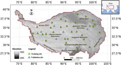
The QTP region is a vast, elevated plateau in central Asia, and its mean elevation reaches 4,000 m above sea level (Zhang et al. 2013) (Figure 1). This region has large numbers of glaciers and lakes that serve as the headwaters for most of the streams and rivers in the surrounding regions, including the three longest rivers in Asia (Yellow, Yangtze, and Mekong Rivers). In this study, we use the QTP boundary provided by Zhang, Li, and Zheng (2002, 2017) to determine the range of the QTP region. The study area covers an area of approximately $2.6\times {10}^6$ km² and is approximately 1,500 km in length from north to south and 2,900 km from east to west.

Figure 1. Study area and the locations of data for model training and validation. The Shuttle Radar Topography Mission (SRTM) elevation data (Farr and Kobrick 2000) are used as the base map.

2.1. Time-series Sentinel-1 SAR images

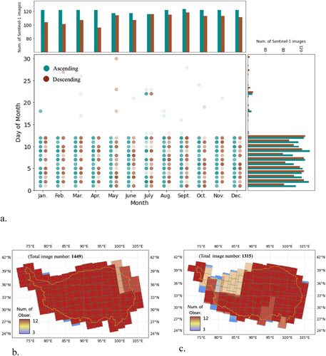
Sentinel-1 is a space mission funded by the European Union and carried out by the European Space Agency (ESA) within the Copernicus Programme. The Sentinel-1A and Sentinel-1B satellites were launched on 3 April 2014 and 25 April 2016, respectively. The two satellites have a repeat observation period of 12 days, so the dual-satellite constellation can provide a repeat period of 6 days. Sentinel-1 collects C-band synthetic aperture radar (central frequency of 5.404 GHz) imagery with a variety of ground resolutions depending on the acquisition mode and processing level. Sentinel-1 Ground Range Detected (GRD) scenes in interferometric wide swath (IW) acquisition mode and 10-m spatial resolution are used for our study. The Sentinel-1 C-band SAR instruments support operation in single (HH or VV) and dual polarizations (HH + HV or VV + VH). The Sentinel-1 data follow the polarization scheme; that is, HH + HV or HH polarization data are mostly used for the monitoring of polar environments and sea ice zones, while VV + VH or VV polarization data are used for other observation zones. With the accessible data archive corresponding to our study region, VV + VH images in IW mode are collected for surface water mapping in this study. In total, we acquired 2,756 dual-polarization (VV + VH) images in 2020 (Figure 2). Even though the QTP region can be fully covered by the Sentinel-1 images in each month, there are still gaps in acquiring both ascending and descending images for a specific region and month. As demonstrated in Figure 2, the accessible ascending data are richer than the descending data for the QTP region. For most of the QTP region that is covered by both Sentinel-1 ascending and descending images, simple image stacking is performed on the acquired ascending and descending images, and the stacked Sentinel-1 image is applied for monthly surface water mapping accordingly.

Figure 2. Space-time distribution of the acquired Sentinel-1 images. a. Temporal distribution of acquired Sentinel-1 images in ascending and descending tracks. The high transparency of the color represents that fewer images are collected on a specific day of the year. b. Spatial distribution of ascending observations. c. Spatial distribution of descending observations.

2.2. SAR-based surface water labeled dataset

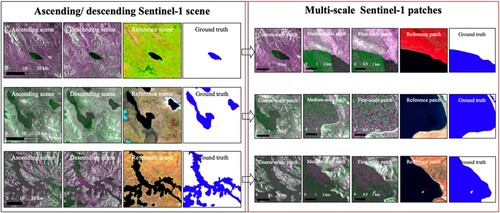
We built an SAR-based surface water dataset for multiscale feature learning of surface water. The dataset contains 39 pairwise Sentinel-1 scenes and ground truths, which are collected at different sites across the QTP (Figure 1). Each Sentinel-1 scene is composed of ascending and descending images, and the pairwise scenes of the dataset are mostly in a very short time interval within 7 days. The surface water boundaries are delineated manually on the screen based on both ascending and descending images. To avoid false determination for the unclear region, the optical Sentinel-2 image with a close acquisition time to the Sentinel-1 scene is used for reference. The extremely difficult-to-recognize water bodies, which are mainly caused by the low signal-to-noise ratio and the limited spatial resolution of the Sentinel-1 image, are excluded from our dataset. The Sentinel-1 scenes have image sizes larger than $3000\times 3000$ pixels; thus, they can be further cropped into multiscale patches with varying numbers and sizes. In this study, we set three scales as $2048\times 2048$, $512\times 512$, and $256\times 256$ pixels. The samples of the pairwise multiscale Sentinel-1 scenes as well as the ground truths and the Sentinel-2 optical scenes are shown in Figure 3 below. In the model testing stage, we divide the dataset into training and validation parts, which consist of 32 Sentinel-1 scenes and 7 Sentinel-1 scenes, respectively. Specifically, to make the training data and validation data independent, thus guaranteeing the reliability of the validation result and making the validation data representative of the whole QTP region, the validation scenes are selected by following the rule of randomness and geographical dispersion in our study. Since more labeled data are used to train the deep learning model, better performance is usually achieved by the trained model; therefore, in the model deployment stage, the fully labeled dataset is used for model training, and the fully trained GMNet is used for monthly surface water mapping in the QTP region.

Figure 3. Demonstration of the Sentinel-1 SAR image-based surface water dataset. Sentinel-1 scene is visualized with a color composite of the VV band (R)-VH band (G)-VV band (B), and the reference Sentinel-2 scene is visualized with a false-color composite of NIR (R)-Red (G)-Green (B).

3. Methodology

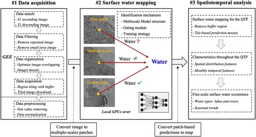
We perform monthly surface water mapping on the QTP, and the spatiotemporal analysis is described as follows. In general, we conducted our study in 3 steps (Figure 4): 1) automatic data acquisition with the Google Earth Engine (GEE) platform, 2) surface water mapping using the deep learning method, and 3) spatiotemporal analysis of the surface water. To obtain highly accurate surface water maps, we design a novel gated multiscale ConvNet (GMNet) for water body identification in this study. The source code of our method is open access and available at https://github.com/xinluo2018/Tibet-Water-2020.git.

Figure 4. The workflow of our study. GEE: Google Earth Engine; S1: Sentinel-1 satellite.

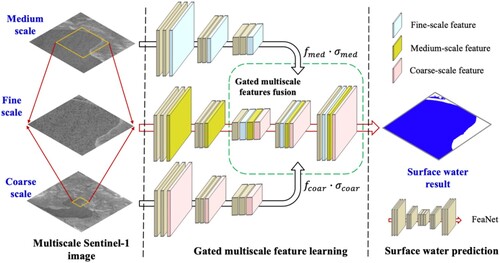
3.1. Framework of the gated multiscale ConvNet

Multiscale information from satellite images is usually beneficial for more accurate identification of the land cover category. In this study, the surface features corresponding to coarse, medium, and fine scales are captured through a structured convolutional module (named the FeaNet module). In general, features from different scales do not contribute to the image recognition accuracy of equivalence. Accordingly, we introduce a gating mechanism to control the multiscale feature flow. We suggest that the multiscale features that can improve surface water identification can pass through the gate and thus be used for better surface water mapping. Multiscale feature gating and surface water classification are performed through a structured convolutional module (the GateNet module) in this study, and the FeaNet and GateNet modules constitute the newly developed GMNet model.

Specifically, we use $X$ to refer to the input data and $w$ to refer to the weights for convolutional computing. Through convolutional computing, the input $X\in {\mathbb{R}}^{H\times W\times C}$ can be mapped to the feature map $f\in {\mathbb{R}}^{H\times W\times C}$ by. (1) $f=w\ast X$(1) where $\ast$ denotes convolution; $f_l=[f_{l1},f_{l1},\dots ,f_{ln}{]}^T$ represents multiscale features in the $l$-th layer; and $n$ is the number of scales of input data, which is set to 3 in our study. In the decoder part of the structured model, the multiscale features that have passed through gating modules are concatenated on the mainstream with skip connections. We use ${\sigma }_l=[{\sigma }_{l1},{\sigma }_{l1},\dots ,{\sigma }_{ln}{]}^T$ to represent the multiscale gate in the $l$-th layer. Then, the concatenated multiscale features can be obtained by (2) $F_l=w\ast \left(w_{l-1}\ast X_{l-1}\circ \left(f_l\mathrm{\Theta }{\sigma }_l\right)\right)$(2) where $F_l$ represents the combined multiscale feature in the $l$-th layer of the decoder part of the structured GMNet model, $\mathrm{\Theta }$ represents the elementwise product, and $\circ$ represents feature concatenation. In the last layer of the GMNet model, a sigmoid function is used to generate the final surface water probability corresponding to each pixel. The overall structure of GMNet is shown in Figure 5.

Figure 5. Structure of the proposed gated multiscale ConvNet.

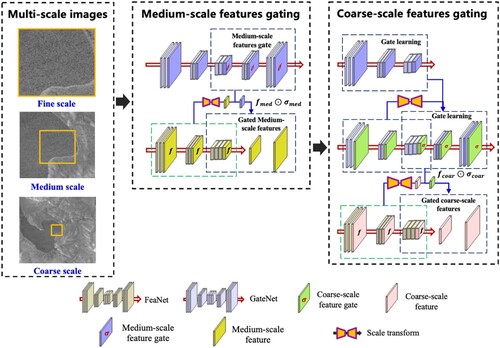
3.2. Multiscale feature gating mechanism

The fine-scale information possesses high ground resolution and is beneficial for fine land cover identification. In the multiscale feature learning of our study, we consider the priorities of scales in the image recognition from fine to coarse, that is, the coarser-scale feature will pass through the gate if the finer-scale feature is unable to accurately separate the surface water from the surface nonwater. We set the fine-scale gate value to a fixed value of 1, and the medium-scale and high-scale gate values are adaptively set as 0–1 through the sigmoid function in the GateNet module. We use $\sigma$ to refer to the feature gate; $w$ and $w^{\mathrm{\prime }}$ are the weights of FeaNet and GateNet, respectively. The subscripts ‘fine’ and ‘med’ represent fine and medium scales, respectively. Therefore, the gated medium-scale feature can be obtained by. (3) ${\mathrm{F}}_{\mathrm{m}\mathrm{e}\mathrm{d}}={\sigma }_{\mathrm{m}\mathrm{e}\mathrm{d}}\cdot {\xi }^{\mathrm{m}-\mathrm{f}\mathrm{i}}\left({\mathrm{f}}_{\mathrm{m}\mathrm{e}\mathrm{d}}\right)=\tau \left({{\mathrm{w}}^{\mathrm{\prime }}}_{\mathrm{f}\mathrm{i}\mathrm{n}\mathrm{e}}\ast {\mathrm{X}}_{\mathrm{f}\mathrm{i}\mathrm{n}\mathrm{e}}\right)\cdot {\xi }^{\mathrm{m}-\mathrm{l}}\left({\mathrm{w}}_{\mathrm{m}\mathrm{e}\mathrm{d}}\ast {\mathrm{X}}_{\mathrm{m}\mathrm{e}\mathrm{d}}\right)$(3) where $\xi$ is a scale transform module to be designed for spatial scope unification of multiscale features by simple cropping and interpolation processing. Here, ${\xi }^{m-fi}$ represents the scale transform from medium to fine scale, and $\tau$ represents the sigmoid function.

Similarly, the coarse-scale feature gate can be derived by the medium-scale feature and fine-scale feature obtained by FeaNet. We use $F_{coar}$ to refer to the gated coarse-scale feature, and it can be obtained through: (4) $\begin{array}{rl}& F_h={\sigma }_{high}\cdot {\xi }^{c-m}\left(f_{coar}\right)\\ & ={\sigma }_{high}\cdot {\xi }^{c-m}\left(w_{coar}\ast X_{coar}\right)\\ & =\tau \left({w^{\mathrm{\prime }}}_{med}\ast \left({\xi }^{m-fi}\left({w^{\mathrm{\prime }}}_{med}\ast X_{med}\right)\circ {w^{\mathrm{\prime }}}_{coar}\ast X_{coar}\right)\right)\cdot {\xi }^{c-m}\left(w_{coar}\ast X_{coar}\right)\end{array}$(4) where the subscript ‘coar’ represents the coarse scale and ${\xi }^{c-m}$ represents the scale transform from coarse scale to medium scale. The workflow to obtain the medium-scale and coarse-scale feature gates is shown in Figure 6.

Figure 6. Gating modules for medium-scale and coarse-scales features, respectively.

Both the FeaNet and GateNet modules are structured with encoder-decoder architecture, and the downsampling (Dsample) and upsampling (Upsample) blocks constitute the basic modules of the network (Table 1). The Dsample block is designed as an inverted residual and linear bottleneck (Sandler et al. 2018); that is, each block consists of a narrow input layer, expanded middle layers, and a narrow output layer. The middle expansion layer consists of depthwise convolutions, which can improve the efficiency of feature learning with lightweight parameters (Howard et al. 2017). The components of Dsample and Upsample blocks are shown in Table 2.

Table 1. ConvNet structure in this study. ‘In’, ‘Ex’, and ‘Out’ represent the numbers of input, exchange, and output channels, respectively.

FeaNet	Description	GateNet	Description
Dsample	Out size: 1/2; In: input image bands; Ex: 32; Out: 16	Dsample,	Out size: 1/2; In: input image bands; Ex: 32; Out: 16
Dsample	Out size: 1/4; In: 16; Ex: 64; Out: 16	Dsample	Out size: 1/4; In: 16; Ex: 64; Out: 16
Dsample	Size: 1/8; In: 16; Ex: 128; Out: 32	Dsample	Size: 1/8; In: 16; Ex: 128; Out: 32
Dsample	Size: 1/32; In: 32; Ex: 128; Out: 32	Dsample	Size: 1/32; In: 32; Ex: 128; Out: 32
Dsample	Size: 1/128; In: 32; Ex: 256; Out: 64	Dsample	Size: 1/128; In: 32; Ex: 256; Out: 64
Upsample	Size: 1/32; In: 192; Out: 64	Gate layer	Conv, 1 × 1, 64, 1; Tanh
Upsample	Size: 1/8; In: 160; Out: 64	Upsample	Size: 1/32; In: 64; Out: 64
Upsample	Size: 1/4; In: 160; Out: 64	Gate layer	Conv, 1 × 1, 96, 1; Tanh
Upsample	Size: 1/2; In: 112; Out: 32	Upsample	Size: 1/8; In: 96; Out: 64
Upsample	Size: 1; In: 80; Out: 32	Gate layer	Conv, 1 × 1, 96, 1; Tanh
Out layer	Conv, 1 × 1, 32, 1; Sigmoid	Upsample	Size: 1/4; In: 96; Out: 64
		Gate layer	Conv, 1 × 1, 80, 1; Tanh
		Upsample	Size: 1/2; In: 80; Out: 32
		Gate layer	Conv, 1 × 1, 48, 1; Tanh

Table 2. Layers of the Dsample and Upsample modules.

Dsample module (In, Ex, Out)	Out size	Upsample module (In, Out)	Out size
avg_pool;	$\times 1/2$ or$\times 1/4$		$\times 2$ or$\times 4$
conv, 3 × 3, In, Ex;		upsample, x2 (or x4), Nearest;
		dwconv, 3 × 3, In, In;
dwconv, 3 × 3, Ex, Ex;		dwconv (optional), 3 × 3, In, In;
dwconv (optional), 3 × 3, Ex, Ex;		conv, 3 × 3, In, Out;
conv, 1 × 1, Ex, Out;

3.3. Data augmentation

We perform min–max data normalization and conventional data augmentation during model training. A dynamic data augmentation strategy is performed in our study, that is, the data is augmented before each batch of training data are fed into the model, and we set the augmentation probability for each batch of training data to 0.2 in our study. The data augmentation methods are described as follows:

1. Random color jitter: We perform random color jitter by following $f\left(x\right)=\alpha \cdot f\left(x\right)+\text{β}$, and the contrast and brightness parameters $\alpha$ and $\text{β}$ are randomly generated within $0\sim 0.05$ during data augmentation.

2. Random rotation and flipping: As commonly used data augmentation methods, random horizontal and vertical flipping and random rotation at angles of [${90}^{\circ }$, ${180}^{\circ }$, ${270}^{\circ }$] are applied.

3. Random noise: We add Gaussian noise to the training data during the training process, and the random standard deviation of the Gaussian noise is within 0∼0.1.

4. Random band missing: We perform band missing augmentation for the Sentinel-1 images: the ascending bands or descending bands are randomly discarded in a randomly determined region.

5. Random region missing: We carry out a region-missing augmentation for the multiscale input patches, i.e. the input patch is masked in a random local region, and the height and width of the maximum masked region are less than 1/6 of the height and width of the patch size.

6. Random line missing: The Sentinel-1 images sometimes appear as invalid edges, which is similar to missing line data; this phenomenon is also reported by Liang et al. (2021). To make the trained model applicable for any Sentinel-1 image, random line-missing augmentation is carried out in our study, and the width and length are randomly set to $1\sim 3$ pixels and $>50$ pixels, respectively.

3.4. Training strategy

We train our model using the Adam optimizer with ${\text{β}}_1=0.9$ and ${\text{β}}_2=0.999$. We set the initial learning rate to 0.0002, and the learning rate is dynamically reduced by a factor of 0.6 when no improvement is seen in the training loss metric for 20 epochs. We use binary cross entropy to measure the training loss, and a regularization technique of label smoothing (Szegedy et al. 2016; Müller, Kornblith, and Hinton 2019) with $\alpha =0.05$ is implemented on the dataset for training loss calculation. Additionly, the overall training epochs and batch size are set to 300 and 16 in our study.

3.5. Evaluation metrics

We evaluate the performance of the proposed method by using recall, precision, overall accuracy (OA), and intersection-over-union (IoU) metrics. The recall metric reflects the probability that a surface water pixel is correctly classified, and the precision metric reflects the probability that a pixel classified as surface water is correct. The IoU represents the area of overlap divided by the area of union between the prediction area and the actual area. The OA metric measures classification quality by combining both the surface water and surface land classification accuracies. IoU is one of the most basic metrics for evaluating the performance of image semantic segmentation, and it can be calculated with. (5) $IoU={\displaystyle \frac{P_{water}\cap T_{water}}{P_{water}\cup T_{water}}}$(5) where $P_{water}$ and $T_{water}$ represent the prediction area and the ground truth area for the surface water body.

4. Results and discussion

4.1. Accuracy assessment for the proposed method

The proposed GMNet is evaluated based on the seven selected validation sites on the QTP (Figure 1). We selected two state-of-the-art SAR-based water extraction methods for comparative analysis. One is the MS-Deeplab method, which is proven to be better than the other mainstream methods, including PSPNet, U-Net, and the original DeeplabV3 + models (Wu et al. 2022), and the other is the HRNet method, which is proven to be better than the DenseNet121, SegNet, ResNet101, DeeplabV3+, OTSU, BTS, FCN, U-Net, and DeepUNet methods (Dong et al. 2021; Kim et al. 2021). According to the accuracy assessment illustrated in Table 3, the proposed GMNet obtained a slightly lower precision of 97.59% compared with the highest precision of 97.72% obtained by MS-Deeplab. While the proposed GMNet achieved the highest recall of 90.50%, IoU of 88.51% and OA of 98.07%, through comparison with the second-highest recall of 85.27%, IoU of 83.52%, and OA of 97.49% obtained by the other methods, the new proposed GMNet method shows significant superiority over the existing methods.

Table 3. Accuracies of the surface water map derived by GMNet and the comparison methods.

Metric (%)	Recall	Precision	IoU	OA
MS-Deeplab	79.00	97.72	77.40	96.23
HRNet	85.27	97.63	83.52	97.49
GMNet	90.50	97.59	88.51	98.07

The detailed accuracy assessment for each validation site is performed to further illustrate the surface water mapping performance of the proposed GMNet method. As illustrated in Table 4, the proposed GMNet achieves high accuracies at the validation sites. Specifically, the mean values of the recall, precision, OA and IoU metrics are all above 88%. The accuracies vary with the specific conditions at the validation sites (e.g. landscape and topography). Among the validation sites, validation site 7 achieves the highest OA (> 99%) in surface water mapping. On the other hand, the model outputs also show serious misclassifications at validation site 4. Specifically, the low recall value indicates that there are many omission errors in surface water classification. Nonetheless, the model still achieves a high OA (97.10%) for the derived surface water map at validation site 4 due to the accurate classification of nonsurface water.

Table 4. Accuracies of the surface water map derived by GMNet for the validation sites.

Metric (%)	Validation sites
	1	2	3	4	5	6	7	Mean
Recall	99.05	93.68	73.79	68.98	99.27	98.98	99.58	90.50
Precision	97.19	93.67	97.91	97.82	97.59	99.32	99.62	97.59
IoU	96.29	88.26	72.65	67.94	96.9	98.31	99.20	88.51
OA	99.54	98.57	92.24	97.10	99.72	99.60	99.72	98.07

4.2. Ablation analysis of the proposed method

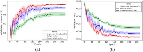
We evaluate the effectiveness of our method through ablation analysis. Generally, the novelty of our ConvNet includes the following: 1) we designed a multiscale ConvNet structure to integrate multiscale information for surface water mapping and 2) we introduced a gating mechanism to determine the feature importance of different scales. We perform an ablation analysis to evaluate the improvements of the novelties in surface water mapping; that is, a comparative analysis is performed among the gated multiscale ConvNet model, the multiscale ConvNet and the single-scale ConvNet to illustrate the effects of the multiscale ConvNet structure and the gating mechanism. We selected a popular DeepLabV3+ (Chen et al. 2018) model to represent the single-scale ConvNet. Because accuracy fluctuations exist in different model training processes, we train each model 10 times, and the statistical results of each metric are obtained. We use the IoU and model loss values to monitor the model performance during model training. As illustrated in Figure 7, the model performance becomes stable when the training epoch reaches 200, and the proposed gated multiscale model maintains the best performance in the on-going model training. More specifically, according to validation accuracy and model loss metrics, the multiscale model outperforms the single-scale model, and the gated multiscale model outperforms the multiscale model, which demonstrates that both the multiscale model structure and the gating mechanism achieved significant improvements in SAR-based surface water mapping.

Figure 7. Comparison of model performances during model training. (a) and (b) correspond to validation accuracy and model loss value metrics, respectively.

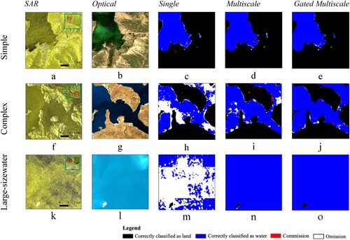
The surface water bodies vary in type, size, and shape, and the background nonwater surface varies in land cover category and topography, thus making it challenging to accurately extract water bodies from Sentinel-1 images. For easily recognized scenes (e.g. Figure 8a, b, c, d, e), the single-scale, multiscale and gated multiscale models can correctly separate the surface water body from the background. For complex scenes, such as rugged terrain areas (Figure 8f, g, h, i, j), SAR images experience layover, foreshortening and shadow issues, which result in missing information on the Earth’s surface. For this complex scene, the single-scale model performs poorly in surface water mapping, as shown in Figure 8h, and many omissions exist in the derived result. The multiscale model achieves improved results while still experiencing some omissions (Figure 8i). The gated multiscale model performs the best and obtains the fewest misclassifications in the produced surface water map (Figure 8j). Taking a large lake as an example (Figure 8k, l, m, n, o), the local scenes are fully occupied by a water body, and this situation leads to background information missing. Accordingly, it is challenging to determine the land cover category in the image. As shown in Figure 8m, since only the local-region patch is adopted for model training, the single-scale model performs poorly in surface water extraction. With the integration of the fine-, medium-, and coarse-scale information of the image, both the multiscale and gated multiscale models achieved high-precision surface water extraction.

Figure 8. Illustrations of surface water mapping for the easily recognized scene, complex scene, and large-size water body scene. Panels a, f and k are the Sentinel-1 images for the three scenes. The green and red boxes represent a larger-scale scene and the location of the visualized scene in the larger-scale scene. Panels b, g and l are the Sentinel-2 images used for references. Panels c, h and m are the results derived by the traditional single-scale deep learning model. Panels d, i and n are the results derived by the multiscale deep learning model. Panels e, j and o are the results derived by the gated multiscale deep learning model.

4.3. Model performance evaluation with different image acquisitions

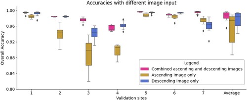
We applied both the ascending and descending Sentinel-1 images rather than only a single ascending or descending image for surface water mapping on the QTP region; therefore, the effectiveness of the combined images in surface water mapping was evaluated in this section. The combination of ascending and descending images provides more information to potentially improve the surface water mapping accuracy, while the data combination also brings redundant information and thus leads to uncertainty and computational burdens in data processing. To verify whether it is indeed effective in improving surface water mapping by simply combining ascending and descending Sentinel-1 images, we compared the performances of the proposed models trained on ascending images only, descending images only, and combined ascending and descending images. Since accuracy fluctuation exists in different training processes, we trained the model 10 times in correspondence to different image acquisition cases, and the comparison among different validation results was followed.

According to the average accuracy among the seven validation sites (Figure 9), the model trained on the combined ascending and descending images achieved the best performance, and the model trained on the ascending images only performed the worst. Nevertheless, the model trained on the combined ascending and descending images does not always outperform those trained on the ascending or descending images only. Among the seven sites, the model trained on descending images only outperformed the model trained on the combined ascending and descending images at sites 4 and 6.

Figure 9. Comparison among models with training on ascending images only, descending images only, and combined ascending/descending images.

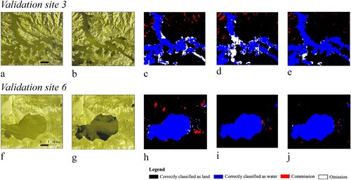
We conduct qualitative analyses for sites 3 and 6, which correspond to the following two situations: 1) the model trained using combined ascending and descending images outperforms the model trained on the single-orbit image and 2) vice versa. As shown in Figure 10, site 3 has very rugged terrain, and the acquired image is covered with a large amount of shadow. Since the ascending and descending images provide information from different views and thus compensate for the missing information from each other in the shadow and layover regions, the model trained on the combined ascending and descending images is superior to the model trained on the single-orbit images only. Validation sites 4 and 6 are both relatively flat and thus are not greatly affected by shadows. We take site 6 as an example (Figure 10). The descending image shows high quality in separating the surface water from the nonsurface water background, while the ascending image is contaminated with noise, thus making surface water indistinguishable from the nonsurface water background. The obtained surface water maps follow human intuition and show that the descending image-based surface water map is comparable to the combined ascending and descending image-based surface water map, and both are superior to the ascending image-based surface water map. Since dense high mountains are distributed in the QTP region, in this study, the model trained on the combined images is regarded as the main model for surface water mapping. For the regions in which we could not acquire both ascending and descending images in a specific month, the model trained on single-orbit images was applied for surface water mapping.

Figure 10. Comparisons of the surface water maps for validation site 3 that are derived from the trained models with different Sentinel-1 image acquisitions. a and f are Sentinel-1 ascending images; b and g are Sentinel-1 descending images; c and h are water maps derived from the trained model with ascending images only. d and i are water maps derived from the trained model with descending images only. Finally, e and j are water maps derived from the trained model with both ascending and descending images.

5. Monthly surface water analysis for the QTP region

5.1. A glimpse of the surface water in the QTP region

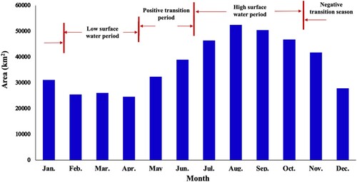
We train GMNet on all the Sentinel-1 scenes of the dataset, and the fully trained GMNet model is applied for month-by-month surface water mapping on the QTP. Accordingly, monthly surface water maps at a 10 m spatial resolution are generated. We calculated the surface water area in each month, and the seasonal variabilities in 2020 were obtained (Figure 11). The surface water area shows dramatic changes, with a maximum of 52,481.33 km² in August and a minimum of 24,585.62 km² in April. Specifically, from February to April, the QTP region covers a low-level surface water area that is less than 30,000 km². The surface water area increases in May and reaches its peak in August, and the surface water area remains stable above 45,000 km² from July to October. From the peak month of August, the surface water area continually decreases in the following months and returns to the lowest value in April. According to the surface water area trend obtained in this study, we divide one year into four periods corresponding to the surface water area on the QTP, that is, the low surface water period from February to April, the high surface water period from July to October, the positive surface water transition period from May to June, and the negative transition period from November to January.

Figure 11. Monthly surface water area statistics for the QTP.

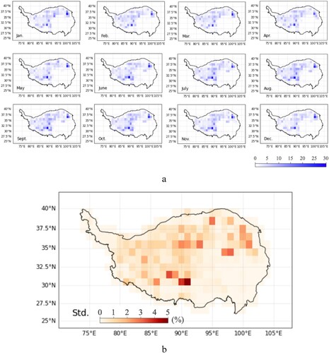
We visually analyze the spatial heterogeneity of surface water in the QTP region in this paper. To enhance the visualization effect, we aggregate surface water within $1^{\circ }\times 1^{\circ }$ tiles. The monthly surface water distribution is illustrated in Figure 12. Generally, the surface water percentage ranges within 30% in different tiles, and the surface water is mainly distributed in the western and northern QTP (Figure 12.a). A possible reason is that the northern and western regions are flat, and therefore, many lakes developed in these regions. We calculate the standard deviation of monthly surface water areas in each tile. As Figure 12.b shows, the tile with more surface water shows larger surface water fluctuation, and the maximum area change reaches 5% of one tile.

Figure 12. Spatial heterogeneity of the monthly surface water in the QTP region. a. the spatially resolved monthly surface water maps, and b. the surface water fluctuation map for the QTP region. The fluctuation is quantified by using the standard deviation metric.

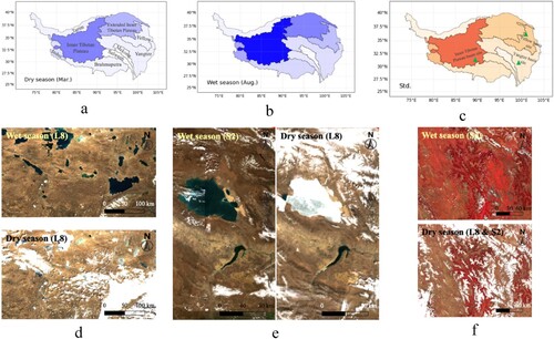
This QTP region mainly consists of 10 hydrological basins (Vörösmarty et al. 2010 and Shean et al. 2020); accordingly, the surface water percentage and the standard deviation of the surface water areas for each hydrological basin are calculated. We use surface water maps in March and August to represent the surface water in the dry season and wet season, respectively. As shown in Figure 13, the Inner Tibetan Plateau basin has the highest surface water percentages in both the dry and wet seasons, and the Mekong basin has the lowest surface water percentages in both the dry and wet seasons. Specifically, the surface water percentages in the Inner Tibetan Plateau basin and Extended Inner Tibetan Plateau basin reach 2.44%, 1.45% and 0.59% in the dry season and 4.73%, 2.43% and 1.69% in the wet season, respectively. According to the standard deviation map in Figure 13, surface water suffers serious fluctuation in the Inner Tibetan Plateau basin, which demonstrates the highest standard deviation of 0.89% of the surface water areas in one year. The surface water in the Mekong basin is stable, which is mainly due to the low surface water percentage in this region. We selected three local sites in different basins to visually analyze the landscape in different regions and periods. According to Figure 13, the Inner Tibetan Plateau basin site and Yellow basin site have high surface water coverage in the wet season, while in the dry season, many of these areas are frozen. The Yangtze Basin site region is mountainous and has little surface water coverage, and there are no significant differences in surface water coverage between the wet season and dry season.

Figure 13. The dynamic surface water features of hydrological basins in the QTP region. a and b represent the surface water percentages of the hydrological basins in the dry season and wet season, respectively. c shows the standard deviation of the surface water areas in each hydrological basin. d, e, and f corresponding to local sites in Inner Tibetan Plateau, Yellow, and Yangtze basins, respectively. L8 and S2 represent the Landsat 8 and Sentinel-2 optical images, respectively.

5.2. Fine-scale analysis of surface water dynamics

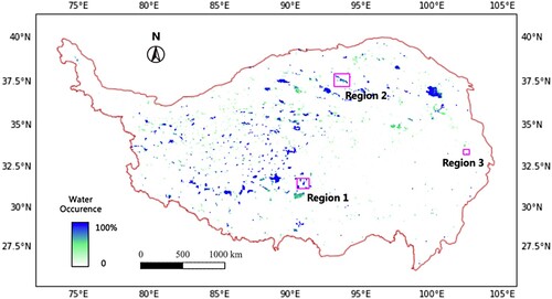
We count the number of pixels that occur as surface water based on the multiple-month surface water maps, and the surface water occurrence for each pixel can be obtained by dividing the number of months in one year (Figure 14). To illustrate the surface water dynamics in the QTP region in detail, we select three local regions for the fine-scale analysis of surface water dynamics. The remote sensing images, including Sentinel-1 ascending and descending images and Sentinel-2 optical images acquired during the cold season and warm season, are also selected to visually analyze the fine-scale surface water variations in this section. We first perform a visual accuracy analysis for the obtained monthly surface water maps. According to visual inspection between the Sentinel-1 images and the obtained surface water maps, the surface water is highly consistent between the surface water maps and the Sentinel-1 images, which demonstrates that the obtained monthly surface water maps are of high quality and are applicable for seasonal surface water dynamic analysis in the QTP region.

Figure 14. Surface water occurrence map in the QTP region.

The selected region 1 is located in the southern QTP region, and this region contains several lakes, such as Dung Tso, Pung Tso, and Sam Tso. As demonstrated in Figure 15, the lakes in this region show different temporal variations; that is, Pung Tso Lake and Dung Tso Lake are relatively stable throughout the year, while Drong Tso Lake and part of Sam Tso Lake show drastic changes within one year. According to the Sentinel-1 ascending images, Pung Tso Lake and Dung Tso Lake maintain similar landscapes in both the cold and warm seasons, while Drong Tso Lake and part of Sam Tso Lake show surface water landscapes in the warm season and nonsurface water landscapes in the cold season. Thus, Drong Tso Lake and part of Sam Tso Lake are frozen in the cold season. This region is extremely representative of most regions of the QTP; that is, frozen surface water is the main reason for surface water fluctuations. Rivers constitute parts of the surface water in the QTP region; therefore, river dynamics are also investigated in detail in this study. As shown in Figure 16, the selected local region contains two rivers: the Yellow River and the Peihe River. Similar to most seasonal surface water bodies in the QTP region, the rivers freeze in the cold season and then melt in the warm season.

Figure 15. Surface water occurrence map for the selected region 1. The green and orange circles represent mutable and stable regions, respectively.

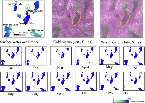
Figure 16. Surface water occurrence map for the selected region 3. The green circle labels a mutable region.

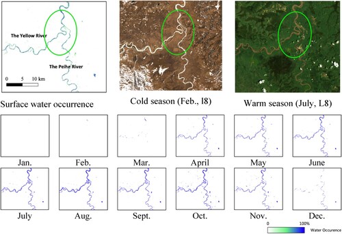
Figure 17. Surface water occurrence map for the selected region 2. The green and orange circles represent mutable and stable regions, respectively.

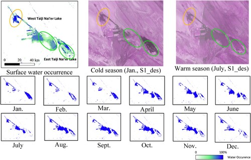
However, there are also surface water changes caused by drought and evaporation in a specific region. As shown in region 2 (Figure 17), the surface water at the top of East Taiji Nai’er Lake is frozen in the cold season, the frozen water melts in the warm season, and the surface water increases accordingly from the cold season to the warm season. Nevertheless, the bottom of East Taiji Nai’er Lake is filled with surface water during the cold season, while the water dries up during the warm season, therefore leading to a decrease in surface water from the cold season to the warm season. A similar finding was also demonstrated by Duan (2018), who mentioned that both West Taiji Nai’er Lake and East Taiji Nai’er Lake underwent drought over time. According to the fine-scale analysis of the surface water dynamics above, the surface water dynamics were usually caused by ice melting and water freezing in the cold season and warm season, respectively. However, the surface water dynamics also show abnormal trends due to drought and evaporation in the QTP region.

6. Conclusion

We proposed a novel deep learning model for surface water mapping based on SAR images. The novelty of the proposed method is that 1) we structured a new convolutional network for multiscale feature learning and 2) we introduced a gating mechanism for more efficient surface water identification by combining multiscale features. According to the validation experiments, the proposed deep learning model achieved high-accuracy surface water mapping; that is, the mean values of the recall, precision, IoU and OA metrics were all above 88%. Through a comparative analysis of methods, the new structured multiscale network and the gated learning mechanism showed significant improvement in surface water mapping. We evaluated the models trained on different Sentinel-1 data acquisitions and showed that the model trained on the combined ascending and descending images outperformed the model trained on the descending image only, and the model trained on the descending image only outperformed the model trained on the ascending image only.

The proposed GMNet model achieved high-accuracy surface water mapping in the QTP region. With the generated monthly surface water maps, the spatiotemporal variations in surface water were explored. According to the dynamic trend in the surface water coverage, we divided one year into four surface water-related periods, that is, the high surface water period from July to October, the negative transition period from November to January, the low surface water period from February to April, and the positive transition period from April to July. For the spatial features of the QTP region, the surface water was mostly distributed in the western and northern Tibetan Plateau region, which is relatively flat and, therefore, developed many lakes. The monthly surface water change showed high consistency with the surface water coverage; that is, the region with high surface water coverage varied greatly over time.

Acknowledgements

We thank Xuanyuan Dong and Yumeng Yin for their efforts in data acquisition and surface water dataset building.

Disclosure statement

No potential conflict of interest was reported by the author(s).

Data availability statement

The Sentinel-1 imagery used in this study is available from the Copernicus Data Space Ecosystem https://scihub.copernicus.eu/ and in Google Earth Engine https://earthengine.google.com/. The monthly surface water dataset generated in this study are available from https://doi.org/10.5281/zenodo.7768932.

Additional information

Funding

This work is supported by the National Natural Science Foundation of China (Proj No. 42001351).

References

- Chen, L. C., Y. Zhu, G. Papandreou, F. Schroff, and H. Adam. 2018. “Lecture Notes in Computer Science.” Proceedings of the European Conference on Computer Vision (ECCV), 833-851.
- Cheng, G., and T. Wu. 2007. “Responses of Permafrost to Climate Change and Their Environmental Significance, Qinghai-Tibet Plateau.” Journal of Geophysical Research 112 (F2), doi:10.1029/2006JF000631.
- Dong, Z., G. Wang, S. O. Y. Amankwah, X. Wei, Y. Hu, and A. Feng. 2021. “Monitoring the Summer Flooding in the Poyang Lake Area of China in 2020 Based on Sentinel-1 Data and Multiple Convolutional Neural Networks.” International Journal of Applied Earth Observation and Geoinformation 102: 102400. doi:10.1016/j.jag.2021.102400.
- Duan, S. 2018. “Lake Evolution in the Qaidam Basin During 1976-2015 and Their Changes in Response to Climate and Anthropogenic Factors.” Journal of Lake Sciences 30: 256–265. doi:10.18307/2018.0125.
- Farr, T. G., and M. Kobrick. 2000. “Shuttle Radar Topography Mission Produces a Wealth of Data.” Eos, Transactions American Geophysical Union 81 (48): 583–585. doi:10.1029/EO081i048p00583.
- Giustarini, L., R. Hostache, P. Matgen, G. J. P. Schumann, P. D. Bates, and D. C. Mason. 2013. “A Change Detection Approach to Flood Mapping in Urban Areas Using TerraSAR-X.” IEEE Transactions on Geoscience and Remote Sensing 51 (4): 2417–2430. doi:10.1109/TGRS.2012.2210901.
- Han, B., and Y. Wu. 2018. “A Novel Active Contour Model Driven by J-Divergence Entropy for SAR River Image Segmentation.” Pattern Analysis and Applications 21 (3): 613–627. doi:10.1007/s10044-018-0702-7.
- Howard, A. G., M. Zhu, B. Chen, D. Kalenichenko, W. Wang, T. Weyand, M. Andreetto, and H. Adam. 2017. “Mobilenets: Efficient Convolutional Neural Networks for Mobile Vision Applications.” arXiv preprint, doi:10.48550/arXiv.1704.04861.
- Huang, W., B. DeVries, C. Huang, M. W. Lang, J. W. Jones, I. F. Creed, and M. L. Carroll. 2018. “Automated Extraction of Surface Water Extent from Sentinel-1 Data.” Remote Sensing 10 (5): 797. doi:10.3390/rs10050797.
- Huo, W., Y. Huang, J. Pei, Q. Zhang, Q. Gu, and J. Yang. 2018. “Ship Detection from Ocean SAR Image Based on Local Contrast Variance Weighted Information Entropy.” Sensors 18 (4): 1196. doi:10.3390/s18041196.
- Huybers, K., S. Rupper, and G. H. Roe. 2016. “Response of Closed Basin Lakes to Interannual Climate Variability.” Climate Dynamics 46 (11): 3709–3723. doi:10.1007/s00382-015-2798-4.
- Immerzeel, W.W., Van Beek, L.P. and Bierkens, M.F. 2010. “Climate Change Will Affect the Asian Water Towers Change Will Affect the Asian Water Towers.” Science 328(5984): 1382-1385. doi:10.1126/science.1183188.
- Insom, P., C. Cao, P. Boonsrimuang, D. Liu, A. Saokarn, P. Yomwan, and Y. Xu. 2015. “A Support Vector Mawchine-Based Particle Filter Method for Improved Flooding Classification.” IEEE Geoscience and Remote Sensing Letters 12 (9): 1943–1947. doi:10.1109/LGRS.2015.2439575.
- Isikdogan, F., A. C. Bovik, and P. Passalacqua. 2017. “Surface Water Mapping by Deep Learning.” IEEE Journal of Selected Topics in Applied Earth Observations and Remote Sensing 10 (11): 4909–4918. doi:10.1109/JSTARS.2017.2735443
- Jiang, W., G. He, T. Long, Y. Ni, H. Liu, Y. Peng, K. Lv, and G. Wang. 2018. “Multilayer Perceptron Neural Network for Surface Water Extraction in Landsat 8 OLI Satellite Images.” Remote Sensing 10 (5): 755. doi:10.3390/rs10050755.
- Kim, M. U., H. Oh, S. J. Lee, Y. Choi, and S. Han. 2021. “A Large-Scale Dataset for Water Segmentation of SAR Satellite.” 2021 IEEE/RSJ International Conference on Intelligent Robots and Systems (IROS), IEEE: 9796-9801.
- Laird, N., A. M. Bentley, S. A. Ganetis, A. Stieneke, and S. A. Tushaus. 2016. “Climatology of Lake-Effect Precipitation Events Over Lake Tahoe and Pyramid Lake.” Journal of Applied Meteorology and Climatology 55 (2): 297–312. doi:10.1175/JAMC-D-14-0230.1.
- LeCun, Y., Y. Bengio, and G. Hinton. 2015. “Deep Learning.” Nature 521 (7553): 436–444. doi:10.1038/nature14539.
- Lehner, B., and P. Döll. 2004. “Development and Validation of a Global Database of Lakes, Reservoirs and Wetlands.” Journal of Hydrology 296 (1-4): 1–22. doi:10.1016/j.jhydrol.2004.03.028.
- Lei, Y., T. Yao, B. W. Bird, K. Yang, J. Zhai, and Y. Sheng. 2013. “Coherent Lake Growth on the Central Tibetan Plateau Since the 1970s: Characterization and Attribution.” Journal of Hydrology 483: 61–67. doi:10.1016/j.jhydrol.2013.01.003.
- Lei, Y., T. Yao, K. Yang, Y. Sheng, M. Kleinherenbrink, S. Yi, B. Bird, X. Zhang, L. Zhu, and G. Zhang. 2017. “Lake Seasonality Across the Tibetan Plateau and Their Varying Relationship with Regional Mass Changes and Local Hydrology.” Geophysical Research Letters 44 (2): 892–900. doi:10.1002/2016GL072062.
- Lhakpa, D., Y. Qiu, P. Lhak, L. Shi, M. Cheng, and B. Cheng. 2022. “Long-term Records of Glacier Evolution and Associated Proglacial Lakes on the Tibetan Plateau (1976–2020).” Big Earth Data 6 (4): 435–452. doi:10.1080/20964471.2022.2131956.
- Li, Y., S. Martinis, and M. Wieland. 2019. “Urban Flood Mapping with an Active Self-Learning Convolutional Neural Network Based on TerraSAR-X Intensity and Interferometric Coherence.” ISPRS Journal of Photogrammetry and Remote Sensing 152: 178–191. doi:10.1016/j.isprsjprs.2019.04.014.
- Li, S., H. Tan, Z. Liu, Z. Zhou, Y. Liu, W. Zhang, K. Liu, and B. Qin. 2018. “Mapping High Mountain Lakes Using Space-Borne Near-Nadir SAR Observations.” Remote Sensing 10 (9): 1418. doi:10.3390/rs10091418.
- Li, N., R. Wang, Y. Liu, K. Du, J. Chen, and Y. Deng. 2014. “Robust River Boundaries Extraction of Dammed Lakes in Mountain Areas After Wenchuan Earthquake from High Resolution SAR Images Combining Local Connectivity and ACM.” ISPRS Journal of Photogrammetry and Remote Sensing 94: 91–101. doi:10.1016/j.isprsjprs.2014.04.020.
- Liang, D., H. Guo, L. Zhang, Y. Cheng, Q. Zhu, and X. Liu. 2021. “Time-series Snowmelt Detection Over the Antarctic Using Sentinel-1 SAR Images on Google Earth Engine.” Remote Sensing of Environment 256: 112318. doi:10.1016/j.rse.2021.112318.
- Liang, D., H. Guo, L. Zhang, H. Li, and X. Wang. 2022. “Sentinel-1 EW Mode Dataset for Antarctica from 2014–2020 Produced by the CASEarth Cloud Service Platform.” Big Earth Data 6 (4): 385–400. doi:10.1080/20964471.2021.1976706.
- Lingyan, C., L. Zhi, and Z. Hong. 2015. “SAR Image Water Extraction Based on Scattering Characteristics.” Remote Sensing Technology and Application 29 (6): 963–969. doi:10.11873/j.issn.1004-0323.2014.6.0963.
- Lu, S., L. Jia, L. Zhang, Y. Wei, M. H. A. Baig, Z. Zhai, J. Meng, X. Li, and G. Zhang. 2017. “Lake Water Surface Mapping in the Tibetan Plateau Using the MODIS MOD09Q1 Product.” Remote Sensing Letters 8 (3): 224–233. doi:10.1080/2150704X.2016.1260178.
- Luo, X., X. Tong, and Z. Hu. 2021. “An Applicable and Automatic Method for Earth Surface Water Mapping Based on Multispectral Images.” International Journal of Applied Earth Observation and Geoinformation 103: 102472. doi:10.1016/j.jag.2021.102472
- Moser, K. A., J. S. Baron, J. Brahney, I. A. Oleksy, J. E. Saros, E. J. Hundey, S. Sadro, et al. 2019. “Mountain Lakes: Eyes on Global Environmental Change.” Global and Planetary Change 178: 77–95. doi:10.1016/j.gloplacha.2019.04.001.
- Mulch, A., and C. P. Chamberlain. 2006. “The Rise and Growth of Tibet.” Nature 439 (7077): 670–671. doi:10.1038/439670a.
- Müller, R., S. Kornblith, and G. E. Hinton. 2019. “When Does Label Smoothing Help?” Advances in Neural Information Processing Systems, 32. doi:10.48550/arXiv.1906.02629.
- Otsu, N. 1979. “A Threshold Selection Method from Gray-Level Histograms.” IEEE Transactions on Systems, man, and Cybernetics 9 (1): 62–66. doi:10.1109/TSMC.1979.4310076.
- Pritchard, H. D. 2019. “Asia’s Shrinking Glaciers Protect Large Populations from Drought Stress.” Nature 569 (7758): 649–654. doi:10.1038/s41586-019-1240-1.
- Qiao, B., L. Zhu, and R. Yang. 2019. “Temporal-spatial Differences in Lake Water Storage Changes and Their Links to Climate Change Throughout the Tibetan Plateau.” Remote Sensing of Environment 222: 232–243. doi:10.1016/j.rse.2018.12.037.
- Qiu, Y., H. K. Lappalainen, T. Che, S. Sandven, and T. Zhao. 2022. “Observations and Geophysical Value-Added Datasets for Cold High Mountain and Polar Regions.” Big Earth Data 6 (4): 381–384. doi:10.1080/20964471.2022.2154974.
- Sandler, M., A. Howard, M. Zhu, A. Zhmoginov, and L. C. Chen. 2018. “Mobilenetv2: Inverted Residuals and Linear Bottlenecks.” Proceedings of the IEEE Conference on Computer Vision and Pattern Recognition, 4510–4520.
- Shao, Z., X. Meng, D. Zhu, D. Zheng, Z. Qiao, C. Yang, J. Yu, Q. Meng, and R. Lü. 2008. “Characteristics of the Change of Major Lakes on the Qinghai-Tibet Plateau in the Last 25 Years.” Frontiers of Earth Science in China 2 (3): 364–377. doi:10.1007/s11707-008-0038-5.
- Shean, D. E., S. Bhushan, P. Montesano, D. R. Rounce, A. Arendt, and B. Osmanoglu. 2020. “A Systematic, Regional Assessment of High Mountain Asia Glacier Mass Balance.” Frontiers in Earth Science 7: 363. doi:10.3389/feart.2019.00363.
- Skakun, S. 2010. “A Neural Network Approach to Flood Mapping Using Satellite Imagery.” Computing and Informatics 29 (6): 1013–1024. url:https://www.cai.sk/ojs/index.php/cai/article/view/127.
- Song, C., B. Huang, K. Richards, L. Ke, and V. Hien Phan. 2014. “Accelerated Lake Expansion on the Tibetan Plateau in the 2000s: Induced by Glacial Melting or Other Processes?” Water Resources Research 50 (4): 3170–3186. doi:10.1002/2013WR014724.
- Strozzi, T., A. Wiesmann, A. Kääb, S. Joshi, and P. Mool. 2012. “Glacial Lake Mapping with Very High Resolution Satellite SAR Data.” Natural Hazards and Earth System Sciences 12 (8): 2487–2498. doi:10.5194/nhess-12-2487-2012.
- Szegedy, C., V. Vanhoucke, S. Ioffe, J. Shlens, and Z. Wojna. 2016. “Rethinking the Inception Architecture for Computer Vision.” Proceedings of the IEEE Conference on Computer Vision and Pattern Recognition, 2818–2826.
- Tong, X., X. Luo, S. Liu, H. Xie, W. Chao, S. Liu, S. Liu, A. N. Makhinov, A. F. Makhinova, and Y. Jiang. 2018. “An Approach for Flood Monitoring by the Combined use of Landsat 8 Optical Imagery and COSMO-SkyMed Radar Imagery.” ISPRS Journal of Photogrammetry and Remote Sensing 136: 144–153. doi:10.1016/j.isprsjprs.2017.11.006.
- Twele, A., W. Cao, S. Plank, and S. Martinis. 2016. “Sentinel-1-based Flood Mapping: A Fully Automated Processing Chain.” International Journal of Remote Sensing 37 (13): 2990–3004. doi:10.1080/01431161.2016.1192304.
- Vörösmarty, C. J., P. B. McIntyre, M. O. Gessner, D. Dudgeon, A. Prusevich, P. Green, S. Glidden, et al. 2010. “Global Threats to Human Water Security and River Biodiversity.” Nature 467 (7315): 555–561. doi:10.1038/nature09440.
- Wang, X., Y. Qiu, Y. Zhang, J. Lemmetyinen, B. Cheng, W. Liang, and M. Leppäranta. 2022. “A Lake ice Phenology Dataset for the Northern Hemisphere Based on Passive Microwave Remote Sensing.” Big Earth Data 6 (4): 401–419. doi:10.1080/20964471.2021.1992916.
- Wang, X., F. Siegert, A. G. Zhou, and J. Franke. 2013. “Glacier and Glacial Lake Changes and Their Relationship in the Context of Climate Change, Central Tibetan Plateau 1972–2010.” Global and Planetary Change 111: 246–257. doi:10.1016/j.gloplacha.2013.09.011.
- Wong, C. P., B. Jiang, T. J. Bohn, K. N. Lee, D. P. Lettenmaier, D. Ma, and Z. Ouyang. 2017. “Lake and Wetland Ecosystem Services Measuring Water Storage and Local Climate Regulation.” Water Resources Research 53 (4): 3197–3223. doi:10.1002/2016WR019445.
- Wu, H., H. Song, J. Huang, et al. 2022. “Flood Detection in Dual-Polarization SAR Images Based on Multi-Scale Deeplab Model.” Remote Sensing 14 (20): 5181. doi:10.3390/rs14205181.
- Yao, T., T. Bolch, D. Chen, J. Gao, W. Immerzeel, S. Piao, F. Su, et al. 2022. “The Thaw Beneath our Feet.” Nature Reviews Earth & Environment 3: 1–1. doi:10.1038/s43017-021-00261-w.
- Yao, T., V. Masson-Delmotte, J. Gao, W. Yu, X. Yang, C. Risi, C. Sturm, et al. 2013. “A Review of Climatic Controls on δ18O in Precipitation Over the Tibetan Plateau: Observations and Simulations.” Reviews of Geophysics 51 (4): 525–548. doi:10.1002/rog.20023.
- Yao, T., L. G. Thompson, V. Mosbrugger, F. Zhang, Y. Ma, T. Luo, B. Xu, et al. 2012. “Third Pole Environment (TPE).” Environmental Development 3: 52–64. doi:10.1016/j.envdev.2012.04.002.
- Zeng, L., M. Schmitt, L. Li, and X. X. Zhu. 2017. “Analysing Changes of the Poyang Lake Water Area Using Sentinel-1 Synthetic Aperture Radar Imagery.” International Journal of Remote Sensing 38 (23): 7041–7069. doi:10.1080/01431161.2017.1370151.
- Zhang, X., N. W. Chan, B. Pan, X. Ge, and H. Yang. 2021. “Mapping Flood by the Object-Based Method Using Backscattering Coefficient and Interference Coherence of Sentinel-1 Time Series.” Science of The Total Environment 794: 148388. doi:10.1016/j.scitotenv.2021.148388.
- Zhang, Y., B. Li, and D. Zheng. 2002. “A Discussion on the Boundary and Area of the Tibetan Plateau in China.” Geographical Research 21 (1): 1–8. doi:10.11821/yj2002010001.
- Zhang, Y., H. Ren, and X. Pan. 2017. “Integration dataset of Tibet Plateau boundary” (dataset). National Tibetan Plateau Data Center, Accessed June 11, 2019.
- Zhang, G., T. Yao, W. Chen, G. Zheng, C. K. Shum, K. Yang, A. Piao, et al. 2019. “Regional Differences of Lake Evolution Across China During 1960s–2015 and its Natural and Anthropogenic Causes.” Remote Sensing of Environment 221: 386–404. doi:10.1016/j.rse.2018.11.038.
- Zhang, G., T. Yao, H. Xie, S. Kang, and Y. Lei. 2013. “Increased Mass Over the Tibetan Plateau: From Lakes or Glaciers?” Geophysical Research Letters 40 (10): 2125–2130. doi:10.1002/grl.50462.
- Zhang, R., L. Zhu, Q. Ma, H. Chen, C. Liu, and M. Zubaida. 2021. “The Consecutive Lake Group Water Storage Variations and Their Dynamic Response to Climate Change in the Central Tibetan Plateau.” Journal of Hydrology 601: 126615. doi:10.1016/j.jhydrol.2021.126615.