The spatial dynamics of Ukraine air quality impacted by the war and pandemic

ABSTRACT

In recent years, our world has experienced significant disruptions due to the COVID-19 pandemic, and Russia's 2022 invasion of Ukraine, impacting human activities and the global environment. This paper explored air quality changes in Ukraine due to COVID-19, and Russia's invasion of Ukraine using on-demand with a what-you-see-is-what-you-get approach. During the COVID-19 pandemic, strict quarantine policies in Ukraine led to a 2% reduction in tropospheric NO₂ concentration before the lockdown and 4% during the lockdown period. Cities like Kyiv, Donetsk, and Dnipro exhibited reductions of 5%, 11%, and 16%, respectively. Total SO₂ column concentration decreased by 6% before the lockdown and 2.5% during the lockdown period, except in high population density areas. Kyiv showed the highest reduction of 17% in SO₂ concentration, while Donetsk and Dnipro exhibited an 11% reduction. However, during the Russian invasion, there was a significant increase in tropospheric NO₂ concentration in heavily destroyed Kharkiv while most eastern regions experienced a reduction. The total SO₂ column was 48% higher before the war but reduced throughout the country after the war, except for in Kyiv and a few central regions. These findings can contribute to analyzing air pollution and building digital twin simulations for future reconstruction scenarios.

KEYWORDS:

• ukraine war
• air pollution
• pandemic
• climate change
• environment
• spatiotemporal computing
• digital twins

1. Introduction

Air pollution is a major environmental issue that has significant impacts on public health. It is caused by various factors such as industrial emissions, burning of fossil fuels, and natural sources such as wildfires and dust storms. According to the World Health Organization (WHO), ambient air pollution is the world’s leading environmental risk factor, responsible for over 7 million premature deaths annually (WHO 2022). Nitrogen dioxide (NO₂), sulfur dioxide (SO₂), Particulate Matter (PM_2.5/PM₁₀), and ozone (O₃) are among the major air pollutants, which are emitted directly into the air from various sources. Climate change impacts factors such as temperature and atmospheric circulation which in turn influence the concentration of air pollutants (Guttikunda and Jawahar 2014). Recent events such as the Russo-Ukrainian war and the COVID-19 pandemic have also had a significant impact on air pollution levels in countries, especially Ukraine. Understanding how these events affect air pollution levels is important for mitigating their impact on public health and for informing future policies.

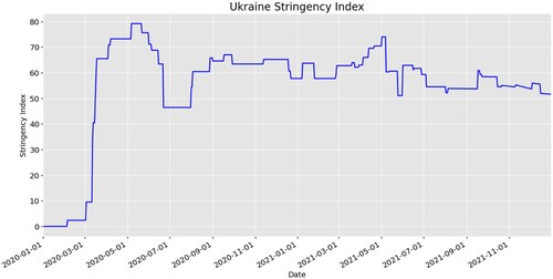
The Russo-Ukrainian Conflict, which began in 2014, intensified with Russia’s invasion of Ukraine on 24 February, 2022. The ongoing conflict has had significant impacts on Ukraine, affecting the country’s economy, environment, and the well-being of its people. The effects of this war are confounded by the concurrent COVID-19 pandemic. Among the many environmental consequences of the conflict, air pollution has emerged as a major concern posing serious risks. During times of war, the usage of weapons such as bombs and missiles, the movement of military vehicles, and damage to power plants, factories, and other facilities can release toxic substances into the air, leading to serious health risks. In addition to the direct harm caused by weapons such as bombs and missiles, the destruction of infrastructure and industries can also contribute to air pollution by releasing particulate matter such as smoke and dust into the atmosphere. Several critical energy infrastructures were attacked as the winter began. Nevertheless, war-imposed restrictions on human movement and disrupted industrial activities, which reduced air pollution. It is important to note that, however, the increased utilization of weaponry also contributed to the release of specific air pollutants. Studies conducted during the COVID-19 pandemic have reported that air pollution levels decreased temporarily in major cities compared to previous years (Torkmahalleh et al. 2021). The reduction in industrial activities and transport during the lockdown period led to a significant reduction in emissions of air pollutants. In the case of Ukraine, the first case was found on 3 March, 2020 (Kyrychko, Blyuss, and Brovchenko 2020). The Ukraine government has implemented many policies to control the spread of the pandemic, including declaring a national emergency, shutting down public stores and services, and imposing mask requirements (Channell-Justice 2023). On 25 March, 2020, the Ukraine government declared a 30-day emergency regime across the country (Åslund 2020). The Ukraine pandemic response policy also corresponds to this evolution of COVID-19, Figure 1 which shows the policy stringency index. The stringency index quantifies the strictness implemented to address the pandemic (Hale et al. 2021). As the pandemic surged again, on 23 September, 2021, the entirety of Ukraine was set back into masking restrictions and other interventions (Pravda 2023). An important air pollution emission source in Ukraine is heavy industry (Sergeeva et al. 2021). The policy stringency index as depicted in Figure 1, suggests that relying on the restoration of polluting industries for the recovery of the Ukrainian economy may result in stagnation (Sha et al. 2021). Studies have found a strong relationship between the impact of air pollution on COVID-19 mortality rates with even a small increase of 1 µg/m³ in PM_2.5 is associated with a significant 15% increase in the death rate (Magazzino, Mele, and Schneider 2020; Wu et al. 2020; Caiazzo et al. 2013). Therefore, it is crucial to study the air quality impact during the COVID-19 pandemic in Ukraine using a spatiotemporal perspective (Yang et al. 2020).

Figure 1. COVID-19 Stringency Index for Ukraine.

Climate change is a global phenomenon affecting all countries, including Ukraine. With its significant level of industrialization, Ukraine faces the challenge of pollutants emitted from transportation and various industries, exacerbating the detrimental effects of climate change on air quality. These impacts can have a range of consequences, including economic losses, infrastructure damage, and harm to human health (Kovalenko et al. 2019). Conversely, climate and weather have strong influences on the spatiotemporal patterns of air pollution. For example, emissions of ozone and PM_2.5 precursors increase at higher ambient temperatures. The reactions that form ozone occur faster with greater sunlight and higher temperatures (Kinney 2018). Due to climate change, air pollution patterns are changing in several urbanized areas over the world with a significant effect on respiratory health (D’Amato et al. 2014). Therefore, the climatic influences on urban air pollution need to be considered or excluded in the analysis procedure to isolate the impacts from the conflicts. It is important to note that the conflict between Ukraine and Russia is irrelated to climate change, but the use of weapons during a war can indirectly impact the environment and climate. Before the Russian and Ukrainian conflict, Ukraine received roughly half of all its power from 15 different nuclear reactors across the country (World Nuclear Association 2023). Attacks against Ukraine’s electric grid infrastructure have caused a 15%−20% energy deficit since 10 October 2022, and Ukraine is now looking elsewhere for power. Improving energy sources involves investing in clean energy technologies, promoting energy efficiency policies, and adopting regulations that encourage renewable energy projects. These energy activities can also affect air quality. Understanding the spatial dynamics of air quality during these situations is significant for knowing their negative consequences on the environment, humans, and economy.

Building upon the preceding paragraph’s exploration of the Ukrainian-Russian conflict, COVID-19, and climate change, it becomes imperative to delve into the analysis and comprehension of the spatiotemporal patterns governing air quality across different scenarios and environments. This includes examining abnormal events, such as the ongoing pandemic and the effects of war, as well as the analysis of heterogeneous big data. Several literature reviews shed light on these important topics.

1.1 Spatiotemporal analytics for events and abnormal detection

Various methods can measure and monitor air pollution, such as in-situ sensors, satellites, and computer models. Spatiotemporal pattern mining or event detection (Yu et al. 2020) can detect changes in air pollution levels by extracting meaningful patterns from accumulated datasets (Guralnik and Srivastava 1999). Event detection is a data mining method used in many applications such as social media, sensor networks, urban traffic, and video streams (George et al. 2021; Guille and Favre 2015; Souto and Liebig 2016; Medioni et al. 2001). Spatial and temporal dimensions are critical for event detection (Kisilevich et al. 2010) and extracting patterns. It is a complex process that involves dynamically tracking event clusters varying in space and time dimensions and exhibiting strong correlations (Yin, Hu, and Yang 2009; Yu et al. 2020). In a dynamic and context-dependent environment, the sensor observations change rapidly resulting in an unprecedented and non-conforming pattern in the target variables. These non-conforming patterns are referred to as anomalies. Anomaly detection refers to the analytics of finding unusual patterns in the data that do not conform to normal behavior (Chandola, Banerjee, and Kumar 2009). Both event detection and anomaly mining are important for this study. For example, several studies have investigated the changes in air pollution anomalies across different regions and timescales, including California (Liu et al. 2021a), India (Liu et al. 2022), and globally (Liu et al. 2021b), as well as nighttime light variations in China before, during, and after the COVID-19 pandemic (Liu et al. 2020). Through the detection and quantification of the air pollution difference between the pandemic years and historical data, the influence of COVID-19 mitigation policies on air pollution is analyzed. We utilized spatiotemporal statistics to identify the anomalies and patterns in this paper.

1.2 Relationships between the pandemic and air quality

Since the declaration of the global pandemic by the World Health Organization (WHO) on 11 March, 2020, research has shown that air pollution significantly decreased during this time. Isaifan (2020) attributed this reduction to lockdown measures and the shutdown of industries, which led to a decrease in air pollutants and associated deaths caused by air pollution. Rodríguez-Urrego and Rodríguez-Urrego (2020) investigated PM_2.5 emission levels in the 50 most polluted cities in the world during the pandemic and found that emissions decreased by 12% globally and locally. Liu et al. (2021a), investigated the impact of COVID-19 interventional policies on the environment by comparing the tropospheric NO₂ in 2020 with the previous five years’ data in California. According to the study, there was a significant drop in the concentrations of NO₂, CO₂, and PM_2.5 during the lockdown period in California. In the past years, air pollution anomaly has been correlated with control policy for controlling the transmission of COVID-19 (Li et al. 2022; Liu et al. 2021a). However, to the best of our knowledge, there are few studies on the air quality impact of the pandemic in Ukraine.

1.3 Relationships between the war and air quality

During a war period, air quality tends to deteriorate because of various factors, such as dust emissions from collapsed buildings, destroyed industries, power plants, explosives, transportation of military vehicles, and combustion of petroleum products. Along with the pollutant emissions, the heat emission from explosives is also a major concern to the environment (Protopsaltis 2012). Studies reported that there was a strong increase in pollutant emissions such as SO₂ after World War II (Nordlund 2000). After the end of World War II, the countries were focusing on the economy and wealth re-boost ignoring the environmental impact (Fenger 1999) that drove up the air pollution. However, in recent times, most countries have strict air quality regulations and policies to monitor and control pollutant emissions mainly in urban areas. While there is limited research on the impact of war on air quality, it is important to note that Ukraine is a highly industrialized country with numerous coal mining industries, chemical and power plants. Destruction of these industries and facilities during conflict may result in adverse effects on the environment, such as the emission of toxic gases into the atmosphere. According to Rawtani et al. (2022), air pollution is one of the short-term impacts of war, while the long-term consequences include the deterioration of people’s well-being due to environmental pollution. Zalakeviciute et al. (2022) analyzed the impact of the Russia-Ukraine war on air quality in Ukraine and Kyiv, finding a significant increase in NO₂ and PM_2.5 emissions during the conflict.

1.4 Spatiotemporal analyses of heterogeneous big data

In recent years, the amount of air quality data has significantly increased due to the proliferation of data from different sources such as monitoring sites, weather stations, in-situ sensors, and airborne and satellite measurements. However, this data is heterogeneous in terms of its format, representation, structure, and size, which poses challenges in storing and processing (Huang et al. 2021). Air quality big data is characterized by the 5Vs of big data (i.e. volume, velocity, variety, veracity, and value), which imply the accumulation of a large volume of data, data generated at high speed with a high temporal resolution, the complexity of data models and representations, consistency and trustworthiness of data, and the value that the data can bring (Demchenko et al. 2013). Air quality data includes geographic and time-series information, making it challenging to apply traditional data mining techniques to air quality analysis. Emerging methodologies and technologies such as distributed file systems, NoSQL databases, and Hadoop-based systems are often used in big data processing and data fusion (Yang et al. 2016a). In general, technical challenges associated with big data include data storage, transmission, analysis, visualization, and privacy (Yang et al. 2016b). The emergence of cloud computing has enabled the critical addressing of the challenges imposed by big data. Specifically, cloud computing offers scalable services, shared and parallel resources, and on-demand platforms that redefine the possibilities of processing and managing big data, especially in geospatial and Earth Science domains (Yang et al. 2016b). A series of spatiotemporal data processing capabilities have been developed, and cloud computing has been utilized to address these challenges.

To understand the air quality impact of the Russia-Ukraine war and the COVID-19 pandemic, this paper analyzes the trends of several air pollutants, including NO₂, SO₂, and O₃, from different aspects, while considering the ongoing effects of climate change. Specifically, we inspected the trends of several air pollutants (i.e. NO₂, SO₂, and O₃) in Ukraine in different contexts to understand how air quality was impacted by the war and the COVID-19 pandemic. Firstly, to investigate the Russia-Ukraine war’s impact on air quality, we considered the air pollutant data from OMI observation from 4 February to March 17, 2022. Additional data is downloaded from 2012 to 2019 for the same period to remove the climatological and seasonal impact. The invasion began on 24 February, 2022. Therefore, in this study, the air quality analysis is conducted by comparing the changes in air pollutants before (4–24 February 2022) and after (25 February–17 March 2022) the conflict start date in a weekly fashion for addressing the missing data when there’s cloud coverage. Secondly, to investigate the impact of COVID-19 lockdown policies on air quality, we considered 11 March, 2020 (the first day of lockdown) as a baseline. We compared the changes in air pollutants before the lockdown (25 February–10 March 2020) and during the lockdown (11–24 March 2020). For the same periods, we downloaded 2012–2019 data to remove the seasonal variations. Hereafter 2012–2019 is termed as Business As Usual (BAU).

To report our research scientifically, we discussed data collected, data collocation, statistical analytics, and the online Ukraine rapid response system in section 2; Section 3 introduces the results and section 4 concludes and discusses future research.

2. Data and methods

2.1 Data collection

2.1.1 War progression

War progression data collection is conducted to track the progress of war based on military operations, casualties and other factors that affect the course of the war. The data collected on the progression of the war in Ukraine from 18 February to 3 November 2022, was compiled from various sources including the Institute for the Study of War’s Ukraine Conflict Updates, NPR, CNN, and Forbes. The data was collected for majorly impacted cities such as Kyiv, Kherson, and Mariupol (Doyle et al. 2023) and compiled into a structured format that detailed each day’s conflicts, cities impacted, conflict zones, damages, global impacts, and the source of the news. The data shows that the city of Kherson was constantly bombarded by Russian troops, which caused many protests by residents. The city of Mariupol was also heavily impacted by the war, with reports of mass graves and forced deportations. The data are synthesized into active or war free for specific regions weekly to temporally match the air quality data.

2.1.2 Air quality datasets

OMI, on board NASA’s Earth Observing System’s (EOS) Aura satellite launched in 2004, is a nadir-viewing UV/Visible spectrometer. The EOS-Aura satellite scans the Earth at an altitude of 705 km in a polar sun-synchronous pattern with a local equator crossing time of 1:45 PM. OMI has a spatial resolution of 13 × 25 km² at the nadir, covers a spectral region of 264–504 nm and provides global coverage every 24 h. With the improved spatial resolution and increased number of wavelengths compared to its predecessors such as the Total Ozone Mapping Spectrometer (TOMS), and Global Ozone Monitoring Experiment (GOME), the OMI products are widely used for trace gas and air quality monitoring from space. In this study, OMI NO₂ tropospheric column (OMNO2d) (Krotkov et al. 2019), OMI SO₂ total column density (OMSO2e) (Li, Krotkov, and Leonard 2020), and OMI O₃ total column density (OMTO3) (Bhartia 2005) are used.

The tropospheric vertical column density (TVCD) NO₂ is calculated by subtracting the slant NO₂ column density from the stratospheric slant column and dividing the result by the tropospheric air mass factor (AMF) (Goldberg et al. 2021). The OMI SO₂ algorithm uses a principal component analysis (PCA)-based spectral fitting algorithm and SO₂ Jacobians to estimate SO₂ vertical column density (Li et al. 2013). The OMI O₃ retrieval algorithm uses the radiance data at the ultraviolet wavelength approximately at 317.5 and 331.2 nm and is based on the enhanced TOMS version 8. The hyperspectral bands in OMI instruments help in reducing the errors caused by uncertainty due to the presence of clouds and aerosols. The OMI Level-3 products are derived from Level-2 product files (usually 14 or 15 orbits) by averaging data over equal grids of dimensions 0.25° × 0.25° for the entire globe. The Level-3 OMI products have pixel level data of good quality that are binned and mapped into a global grid. The screening criteria to generate Level-3 OMI NO₂ is solar zenith angle (SZA) < 85°; cloud-pixels < 30%; cross-track quality flags 0 or 255. Similarly, the screening criteria to generate Level-3 OMI SO₂ is SZA < 700; cloud pixels < 20%; Air Mass Filter (AMF) > 30%.

2.1.3 PM_2.5 data from in-situ sensors

PM_2.5 data are obtained from the Air Quality Index (AQI) China (AQICN 2023) website, which provides real-time air quality data from monitoring stations in many cities worldwide including a few in Ukraine. The PM_2.5 data are downloaded using the AQICN API in a structured format for the period between October 2019 and November 2022 in Ukraine. The data contains the city, date, minimum, maximum, median, and standard deviation of PM_2.5. It should be noted that PM_2.5 data are only available for nine cities in Ukraine.

2.1.4 Ancillary data

TROPOMI is a nadir-viewing push-broom hyperspectral imaging spectrometer mounted on the Sentinel-5P Precursor (S5P) satellite. The satellite orbits the Earth in a sun-synchronous orbit at an altitude of 824 km. It has 8 spectral bands ranging from ultraviolet to short-wavelength infrared. The initial spatial resolution of TROPOMI was 3.5 × 7 km², after 6 August 2019, the spatial resolution was improved to 3.5 × 5.5 km². TROPOMI provides air pollutant measurements of NO₂, SO₂, O₃, methane (CH₄), aerosols, etc. While providing higher resolution and the latest measurements, the historical data archival is not enough for climatology analyses, therefore, we used the TROPOMI NO₂ (KNMI 2018) for limited analyses in this study. To address the no-value problem caused by cloud coverage, we averaged the air quality data on a weekly basis.

2.1.5 Implementation of cloud computing platform for air quality big data processing

Apache Science Data Analytics Platform (SDAP) is a Cloud Computing Spark solution to support Big Data management and analysis in various domains (Huang et al. 2022). In this study, the SDAP is deployed in an OpenStack cloud. Due to the scalable and parallel analytical nature of the SDAP, the air quality Big Data that we downloaded and pre-processed for this study is ingested seamlessly and harmonized for further analysis. The air quality data are generated in NetCDF4 format that has both space and time dimensions. Considering their huge volume and multi-dimensional nature, searching, sub-setting, and retrieving information from these files are challenging. To overcome the above-mentioned challenges, SDAP offers (i) scalable ingestion service, (ii) parallel processing for handling big data, (iii) high-performance geospatial indexing and distributed search solution, (iv) metadata and tiled data generation to remove repetitive file Input/Output (I/O) operations, and (v) collection of web service endpoints for analytical purposes.

2.2 Data preprocessing

To understand the impact of war on air quality, it is necessary to link the air quality data with time and space along with the war progression data. OMI and TROPOMI air quality products have different spatial resolutions, TROPOMI has a better spatial resolution compared to OMI. To make TROPOMI and OMI comparable, they are resampled and remapped to an equal resolution of 0.05° × 0.05° grid. The resampling is performed with the kriging methodology.

2.2.1 Spatial interpolation using kriging

Kriging is a spatial interpolation method that estimates unknown values based on measured values and their correlation properties (Longley et al. 2015). The estimation is done through a weighted mean using a set of known points and measured values. For a given set of known points and measured values at these points, Z(s), the estimation at an unknown location is given by weighted mean: $Z^{\ast }(S_0)=\sum _{i=0}^N{\lambda }_{i}Z(s_i)$

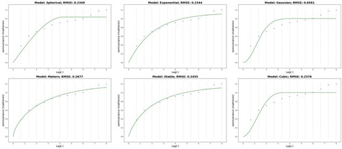
where N is the total number of observations, and λ is the weighted array. To ensure that the model is unbiased with minimized errors, one must properly determine the weights. Variogram models are used to calculate the weights by grouping observations into distance bins and identifying similarities based on spatial proximity. The empirical variogram is modelled to define the spatial pattern. Variogram models include spherical, exponential, gaussian, and matern. The best model is selected based on the lowest root mean square error (RMSE) in this study. $\mathrm{RMSE}=\sqrt{\left[\sum {(P_i-O_i)}^2/n\right]}$

where P_i is the predicted value and O_i is the measured value.

In general, RSME shows a model’s ability to predict the targeted value. The lower the RMSE value, the better the model prediction is. Existing studies have used various interpolation methods to predict the unmeasured values for air quality research. Wei et al. (2022) used a spatiotemporally weighted artificial intelligence technique to fill the data gaps in OMI and TROPOMI data and achieved an RMSE of 0.46 × 10¹⁵–1.51 × 10¹⁵ molecules/cm². The approach presented in our study has demonstrated comparable results, achieving an RMSE range between 0.23 × 10¹⁵ and 0.65 × 10¹⁵ molecules/cm², as depicted in Figure 2.

Figure 2. Variogram models for spatial interpolation used in the study.

2.2.2 Re-gridding of OMI products

The original level-3 daily OMI products have a spatial resolution of 0.25° by 0.25°. The initial step in spatial collocation is to calibrate the raw data pixels with a scaling factor. Then, spatial re-gridding is done by establishing a finer mesh grid of spatial resolution 0.05° by 0.05°. The level-3 weekly products are derived from aggregating daily data of high-quality pixels which are then remapped and re-gridded with the kriging methodology. A detailed mathematical description of generating re-gridding products is discussed in section 2.2.1.

2.2.3 Re-gridding of TROPOMI products

The re-gridding of Sentinel-5P TROPOMI products involves the generation of level-3 data from level-2 products. The conversion process includes considering the time, latitude, and longitude variables of level-2 products, product name and their relevant attributes, and data quality flags. The first step in spatial collocation is to filter the pollutant variable with a data quality flag greater than 50 to remove the cloud pixels. Then, for a given time and spatial coverage, multiple overpasses are accumulated and smoothed on a weekly basis. The next step is to establish a spatial grid of resolution 0.05° × 0.05° covering the Ukraine region. Finally using the best-fitting kriging methodology, we remapped the raw satellite data to a finer resolution.

2.2.4 OMI/TROPOMI correlation

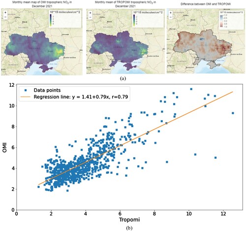
To correlate the NO₂ products from TROPOMI and OMI observations, we generated the re-gridded monthly average map of tropospheric NO₂ data derived from the kriging methodology as shown in Figure 3a. In this study, the discussion is based on December 2021 NO₂ observation. The distinct spatial distribution of tropospheric NO₂ concentration in TROPOMI and OMI is evident from these figures. In general, OMI observation has a higher tropospheric NO₂ concentration compared to TROPOMI. This finding agrees well with the previous studies (Wang et al. 2020; Goldberg et al. 2021). Especially, in eastern regions of the country near the vicinity of highly polluted areas, the OMI NO₂ observation is approximately 0.5 × 10¹⁵ molecules/cm² higher than the TROPOMI NO₂ observation. However, the spatial distribution map of TROPOMI shows hotspots near Kyiv, Lviv, and Donetsk which are not very prominent in OMI. Various factors influence the difference in their observations such as retrieval algorithm, scanning pattern, calibration technique, and most importantly cloud coverage (Wang et al. 2020). Figure 3b shows the scatterplot diagram of tropospheric NO₂ in December between the TROPOMI and OMI data over Ukraine. The linear relationship shows a well-correlated positive relationship with a correlation coefficient of 0.79. For the other months, the correlation went down to 0.50. To conclude, both NO₂ products agree well but their magnitude differs in a polluted region of the country. T-test was used to test the statistical significance of the regression model. The calculated regression coefficient was significantly different from zero (t = −7.33, P < 0.05) which indicates the effectiveness of the regression model.

Figure 3. (a): December 2021 NO₂ observation – OMI, TROPOMI, the difference between OMI and TROPOMI; Figure 3 (b): The correlation between re-gridded OMI and TROPOMI in December 2021 over Ukraine.

2.3 Statistical analysis and anomaly detection

2.3.1 Time series analysis

The time-series analysis is conducted by estimating the area average map of 2022, 2020, and BAU (2012–2019) and comparing the change in patterns of the pollutants. We adopted the time-series methodology discussed by (Liu et al. (2021a). The below section details the time-series calculation steps:

1. The weekly mean is calculated by averaging the daily mean concentration of the pollutants. $W_{\mathrm{t}}={\displaystyle \frac{{\sum }_{i=1}^n{D}_i}{N}}$

Where W_t is the weekly mean concentration of the pollutant, D_i is the daily mean concentration and i is the days in a week. N is the total number of days in a week. For the BAU period, the weekly mean concentration is calculated by averaging each week’s mean concentrations from 2012 to 2019.

b.	Then, the weekly mean concentration values are normalized to the mean before the period of the Russia-Ukraine war which is from 4 February to 24 February. It is calculated by dividing the weekly mean concentration by the mean of the before period. $W_{norm}={\displaystyle \frac{W_t}{W_{Feb4-Feb24}}}$
c.	Finally, the normalized values are compared to differentiate the pollutant trends in three periods.

2.3.2 Spatial distribution analysis (weekly)

The spatial distribution analysis is calculated by estimating the pollutant concentration over a region by averaging each pixel during the study period.

d.	The seasonal influence is removed by calculating the climatological data using the 2012–2021 average. Then, by subtracting the climatological data from the 2022 pollutant concentration, we calculated the anomalies of each pollutant concentration.
e.	Finally, differences among war and BAU periods and COVID-19 and BAU periods are estimated based on the anomalies obtained from the previous step.

2.4 Online Ukraine rapid response system

The Ukraine rapid response system adopted a client-server approach running an on-premises cloud and was developed using the Shiny app. The connection between the client and server is established using an R session. The client requests the server which is served using a WebSocket communication (Figure 4). The dashboard offers an interactive experience to the user in which the user can provide input to the system. Then the system processes the request and responds with the requested information. The Shiny app is hosted using the open-source Shiny server. The Shiny server performs three main operations namely time-series analysis, spatial analysis, and anomaly detection. The data for these operations are retrieved from the Apache Science Data Analytics Platform (SDAP). In this rapid response architecture, SDAP acts as a middle layer that supports and enables scientific investigations and analysis through scalable services and data structures. The Shiny server makes RESTFUL API requests to the SDAP with various search criteria made by the users. For example, the search criteria generally encompass the spatial extent (in bounding box), and time range (start and end time). The SDAP responds in JSON format along with the metadata. On the server side, the response is parsed, and results are rendered as raster images or graphs. It is to be noted that the response time of the SDAP varied according to the search criteria.

Figure 4. Architecture of the Ukraine Rapid Response Dashboard.

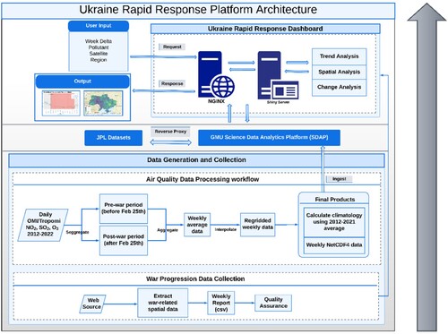
Figure 4 shows the architectural diagram of the Ukraine Rapid Response System. The rapid response platform consumes three analytical services in the SDAP namely (i) area-averaged time series computes the average value of a variable of interest over a series of points between two periods, (ii) time-series spark computes the time series plot between two or more datasets for the variable of interest, and (iii) data in-bounds calculate the area average over a region for a single timeframe.

Figure 5 details the process that the rapid response dashboard uses to retrieve and process the air pollution data from the GMU SDAP. The necessary data for air quality analysis is ingested in NetCDF4 files and retrieved in JSON format upon request.

1. First, the program collects several user inputs into the necessary parameters to call each API. These include the week period, pollutant, region of interest, and the satellite source.

2. Next, the program calls the data in-bounds API which returns the air pollutant values of each point within the desired region and converts the data into a raster format.

3. The user selection indicates the appropriate administrative boundary polygon which is then used to mask the raster to the appropriate spatial coverage.

4. The program then uses the maximum and minimum values of the pollutant concentration that are retrieved using the time-series spark API to make a color bar of the raster data.

5. The program then passes this raster as well as the maximum and minimum values to a leaflet function to create a map of the pollution data.

Figure 5. Air quality analysis workflow for the Ukraine Rapid Response Dashboard.

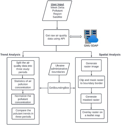
In a parallel process, this program also calls the time-series spark API to get the necessary data for a time-series plot of the pollutant concentration aggregated weekly. The API returns the statistics such as minimum, maximum, mean, and standard deviation of the selected pollutant, region, and satellite source. The data is then processed to assign a flag for the three temporal periods in the study, BAU (2012–2019), COVID-19 (2020), and the present periods in which Ukraine is at war (2022-Present). Once these fields are added to the data, a normalized mean is calculated using the mean of each week and the per-mean value. The pre-mean value is defined as the mean value for the calendar dates before the war started, 4 February–24 February for each period (BAU, COVID-19, and Present). The normalized value allows us to compare individual values for different dates across periods. The program uses normalized mean values to calculate a percent difference between the pollutant concentration for each period and the BAU periods. The normalized mean for each period is then plotted throughout the calendar year using a gpplot2 function and displayed on the Shiny app.

3. Experiment and results

3.1 System implementation and results

To effectively support the analyses of air quality changes in Ukraine, we built the Ukraine rapid response dashboard (ukraine.stcenter.net). This dashboard documents various social and environmental changes in Ukraine because of the war using an interactive web page that dynamically displays information about the concentration of several pollutants including NO₂, SO₂, and O₃. This dashboard reacts to user input and displays a raster map of weekly pollutant concentration, as well as a time series plot and data table of the normalized mean concentration and percent change for the selected region. Figure 6 shows the default view of the air quality analysis tab in the rapid response dashboard with the user input bar on the left side, a raster image overlaid on a leaflet map on the center, and a time-series plot on the right side.

Figure 6. Default View of the Air Quality Analysis Tab.

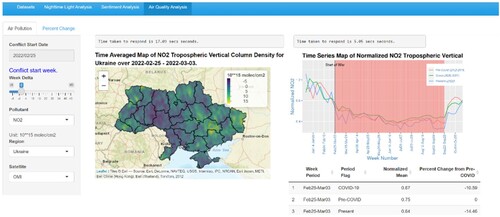
A user can select any input from the sidebar based on which the dashboard reacts to the request. The orange bar in the time-series plot represents the active war period in the region.

3.2 Climate impact on air quality in Ukraine

Although the seasonal and climatology impact on the air quality varies from year to year and season to season (Figures 7a, 8a, and 9a), OMI data shows that the NO₂ levels have slightly declined over the past decade, while levels of O₃ and SO₂ do not show significant long-term trends. Despite control policies, most cities in Ukraine still have emission levels higher than the Maximum Allowable Concentrations (MAC). A long-term average of the years 2012–2019 would help remove the variances and provide a good baseline to compare and obtain meaningful anomalies caused by the industrialization, pandemic, and Ukraine war in the last decade.

Figure 7. (a): NO₂ anomaly derived by removing the climatic average; (b) SO₂ anomaly derived by removing the climatic average; (c) O₃ anomaly derived by removing the climatic average.

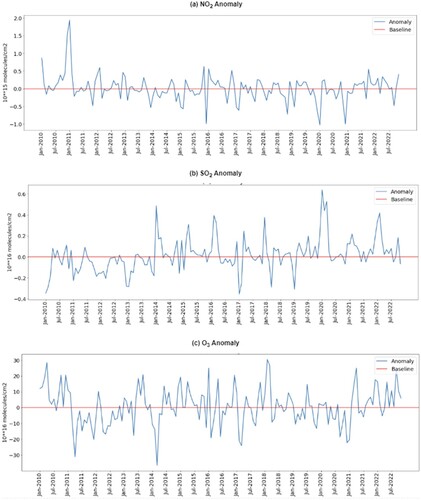
It is evident from Figure 7a–c, that NO₂, SO₂, and O₃ have a clear seasonal pattern, with NO₂ and SO₂ peaks in winter and lower in summer and O₃ peaks in spring and summer. For NO₂, the seasonal trend can be attributed to (i) increased emissions from sources that use fossil fuels for residential heating, energy production, and transportation during wintertime, and (ii) meteorological conditions, such as temperature and atmospheric mixing, and the dispersion of NO₂ in the atmosphere which tends to stay longer in the atmosphere due to less sunlight during wintertime (Bočková et al. 2020). The unusual spikes in early 2011 could potentially be attributed to abnormally hot weather conditions during the preceding summer of 2010, which saw NO₂ concentrations consistently exceed the maximum permissible level. Furthermore, the country was plagued by plumes from a forest fire that occurred in the latter half of 2010 (Zvyagintsev et al. 2011). NO₂ tends to remain in the atmosphere for longer periods during the winter months, and as such, the particularly hot summer and subsequent forest fires in late 2010 could have led to increased emissions of NO₂, which then accumulated in the atmosphere and persisted during the winter months. According to Popov et al. (2020), the emissions of NO₂ increased between 2016 and 2017 in Kyiv from stationary polluting sources which indicates a possible decline in air quality during that period. From Figure 7a, it is shown that the variance in anomalies has reduced considerably since 2014. During 2020, when the COVID-19 pandemic hit the countrywide quarantine was issued on 11 March 2020. Due to the restrictions and the subsequent reduction of anthropogenic activities, the NO₂ anomaly is negative implying the effect of lockdown. In early 2022 (January–February), though the NO₂ is lower than the climatic average, not as low as the same period of the previous year.

According to Bočková et al. (2020), the total SO₂ column demonstrates a seasonal fluctuation, with the highest levels occurring during the winter months of November through January. Meteorological conditions, the absence of vegetation with low precipitation rates, and less tendency of SO₂ to transform into other sulfur compounds during winter are the major contributors to the increase in total SO₂ column (Rogalski et al. 2014). Between 2014 and 2017, the SO₂ concentration varied drastically reaching positive and negative anomalies (Figure 7b). However, in recent years the concentration of SO₂ in the atmosphere is continuously higher than the climatic average. Specifically, during COVID-19 (2020) and during the war period (2022), the SO₂ concentration is 0.6 × 10¹⁶ molecules/cm² and 0.4 × 10¹⁶ molecules/cm² higher than the climatic average.

In general, the volume of the total O₃ column in the atmosphere depends on the frequency of the stratospheric-tropospheric exchange (STE) of ozone (Shin et al. 2020). The STE triggers an increase in ozone concentration in the tropopause that results in high total ozone concentration and surface ozone concentration. Climate change and anthropogenic activities are the major contributors that accelerate the STE. As shown in Figure 7c, during the COVID-19 (2020), the total ozone concentration is lower compared to the climatic average. But in recent years, the ozone concentration exceeds the climatic average by 30 × 10¹⁶ molecules/cm².

3.3 Pandemic impact on air quality in Ukraine

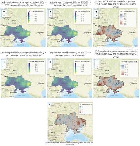
The pandemic impact on air quality is investigated by analyzing the changes in air pollutants during the lockdown period in Ukraine and comparing the air pollutants pattern with the BAU (2012–2019) as discussed in the data and literature review sections. Tropospheric NO₂ concentration before and during the lockdown period over Ukraine are visualized in Figure 8a–d, showing a 2% reduction in NO₂ concentration in 2020 compared to the historical mean (2012–2019) before the lockdown, and a 4% reduction during the lockdown. Industrialized zones such as Donetsk, Luhansk, Dnipro, and Kyiv have high concentrations of NO₂ due to the location of factories and mining industries (Savenets 2021). During the lockdown period, these industrialized cities experienced significant reductions in NO₂ concentration. For instance, Donetsk experienced an 11% reduction, while Kyiv experienced a 5% reduction, and Dnipro experienced a 16% reduction. Figure 8g shows the anomalies of tropospheric NO₂ decreasing significantly in the eastern regions and around Kyiv. This reduction is likely due to the strict quarantine policies that led to a reduction in anthropogenic emissions of tropospheric NO₂. Overall, the findings suggest that the COVID-19 pandemic and subsequent lockdown measures have had a positive impact on air quality in Ukraine.

Figure 8. (a): Average tropospheric NO₂ (2020) before lockdown (b) Average historical tropospheric NO₂ (2012–2019) (c) Before lockdown tropospheric NO₂ anomalies (d) Average tropospheric NO₂ (2020) during lockdown (e) Average historical tropospheric NO₂ (2012–2019) (f) During lockdown tropospheric NO₂ anomalies. Figure 8 (g): Difference between anomalies of before and during the lockdown periods (c–f). 

The spatial distribution of the total SO₂ column before and during the lockdown period over Ukraine is shown in Figure 9a–d. As shown in Figure 9b and 9e over Ukraine, the high SO₂ concentrations are found in southeastern parts of the country which uses high-sulfur content combustion of mining processes (Nádudvari et al. 2021). In addition, southeastern regions are dominated by other major emission sources of SO₂ such as metallurgical and power industries. In the case of 2020, the total SO₂ column is highly heterogenous and varied across the country. The overall total SO₂ column concentration in Ukraine is reduced by 6% in 2020 before lockdown compared to the same period in historical mean (2012–2019). During the lockdown in 2020, the concentration is reduced by 2.5% compared to the same period in historical mean (2012–2019). The city of Kyiv showed a reduction in total SO₂ column concentration by 17%, while the city of Donetsk and Dnipro exhibited a reduction of 11%. As shown in Figure 11g, the anomalies of the total SO₂ column decrease in the southeastern regions of the country. The high population density regions such as Kharkiv, Khmelnytskyi, and Donetsk showed an increase in the total SO₂ column during the lockdown (Figure 9g). Apart from industrial sources, the combustion of sulfur-containing fossil fuels for heating homes is another major of SO₂ emissions (Filonchyk et al. 2020). Due to the stay-at-home order during the lockdown period, the citizens might have stayed at home usual than longer periods using the sulfur-content fossil fuels for heating homes might have attributed to the spike in the high-density areas.

Figure 9. (a) Average tropospheric SO₂ (2020) before lockdown, (b) Average historical tropospheric SO₂ (2012–2019), (c) tropospheric SO₂ anomalies before lockdown, (d) Average tropospheric SO₂ (2020) during lockdown from 11 March–24 March, (e) Average historical tropospheric SO₂ (2012–2019), and (f) tropospheric SO₂ anomalies during lockdown. Figure 9 (g): Difference between anomalies of before and during the lockdown periods (c–f).

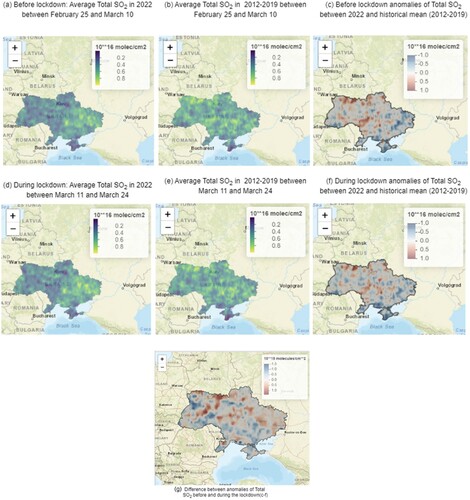
Figure 11. Spatial distribution of tropospheric NO₂ over Kherson, Dnipro, Lviv, and Kharkiv.

3.4 War impact on air quality in Ukraine

To understand the impact of war on air quality, the time-averaged map of Ukraine and cities such as Kherson, Dnipro, Lviv, and Kharkiv are generated from OMI NO₂ and SO₂, data.

3.4.1 Tropospheric NO₂ three weeks before and after the war

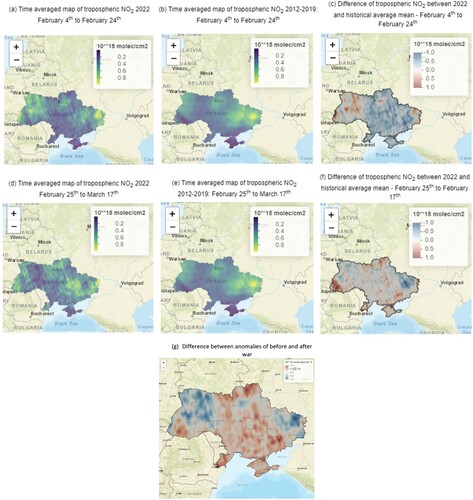
Figure 10a,b,d, and e show the spatial distribution of tropospheric NO₂ over Ukraine for three weeks before the conflict starts (2022 and historical mean) and three weeks after the conflict starts (2022 and historical mean). Generally, the NO₂ concentration is significantly higher in Kyiv and the eastern regions of the country. The high concentration of NO₂ is attributed to the location of thermal plants, chemical industries, and metallurgical industries in these regions (Bočková et al. 2020). Additionally, the high population density in the eastern and southeastern regions such as Donetsk, Luhansk, etc. is associated with the high transportation rate that contributes to the high levels of NO₂ emissions from vehicles. During the three weeks before the war, the NO₂ concentration was uneven throughout. Overall, the NO₂ concentration is higher compared to the historical mean. The mean concentration of NO₂ from 4 February to 24 February is 3.22 × 10¹⁵ molecules/cm². While the historical mean for the same period is 2.64 × 10¹⁵ molecules/cm². The difference map shows that the NO₂ concentration is increased near Kyiv, most of the western regions, and the vicinity of Luhansk oblast. The western regions of the country showed an unusual spike in the NO₂ concentration during this period (Figure 10a). This pattern could be attributed to the initial strikes on February 24th reaching as far as the western region of the country reported by El-Bawab and Raddatz (2023). As the war progressed, the NO₂ concentration between 25 February and 17 March was considerably reduced. The mean concentration of NO₂ is 2 × 10¹⁵ molecules/cm² in 2022 while the historical mean concentration was 2.49 × 10¹⁵ molecules/cm² during the same period. Most of the eastern regions of the country showed a reduction in NO₂ concentration. This reduction can be attributed to the reduction of anthropogenic activities and the shutdown of major industries and power plants as a response to the ongoing war (Zalakeviciute et al. 2022).

Figure 10. Spatial distribution of tropospheric NO₂ over Ukraine. (a)–(b) are time-averaged maps of OMI tropospheric NO₂ concentration from 4 February–24 February 2022, and 2012–2019. (c) difference between the weekly average (before the conflict started) of 2022 and 2012–2019. (d)–(e) are time-averaged maps of OMI tropospheric NO₂ concentration from 25 February–17 March 2022, and 2012–2019. (f) difference between the weekly average (after the conflict started) of 2022 and 2012–2019. Figure 10 (g): Difference between anomalies before and after the war.

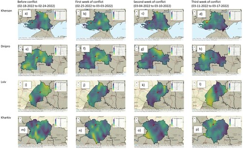
Figure 11a–11p shows the spatial pattern of NO₂ concentration over Kherson, Dnipro, Lviv, and Kharkiv before the war, the first week of the war, the second week of the war, and the third week of the war. Kherson is in the southern portion of Ukraine. It is one of the oblasts in Ukraine that is partially occupied by Russian troops in 2022. The red dot in the first row denotes the location of Kherson city (Figure 11a–11d). Since the commencement of the war, the overall NO₂ concentration in the Kherson oblast has decreased. The normalized mean concentration of NO₂ before one week of the conflict, the conflict start week, a week after the conflict and two weeks after the conflict are 0.98, 0.84, 0.44, and 0.51, respectively. But the perimeter around Kherson city shows a higher concentration of NO₂. Several bombings and air strikes in Kherson airport happened during the first and second weeks of March that could have been attributed to the spike in NO₂ (Zalakeviciute et al. 2022; Khurshudyan and Berger 2023). Dnipro, a central eastern oblast, is currently under the control of Ukraine. It is one of the most industrialized regions of the country. Though it is under Ukraine’s control, the oblast has been attacked by missiles in early March that resulted in casualties. The spatial distribution map of Dnipro from 11 March to 17 March 2022, showed a slight increase in NO₂ concentration during the active war period (Figure 13h). Lviv was one of the cities that was attacked on 24 February by a Russian missile bombing. The normalized NO₂ mean concentrations during the four weeks are 1.22, 0.54, 0.38, and 0.68 × 10¹⁵ molecules/cm² respectively and concentration was increased by 28.35% compared to the historical mean concentration when the invasion started on 24 February (Figure 11i). Kharkiv, a northeastern oblast in Ukraine, is one of the major targets for the Russian invasion and the most destroyed region in Ukraine in terms of both casualties and properties (Khurshudyan and Berger 2023). Specifically, at the beginning of March, the region suffered intensified missile attacks including an attack on a nuclear research facility and city-center square. The attacks caused the destruction and combustion of buildings, residential areas, and administrative buildings. From Figure 11n, the NO₂ concentration is increased considerably throughout the region exceeding 10 × 10¹⁵ molecules/cm².

3.4.2 Total column density SO₂ three weeks before and after the war

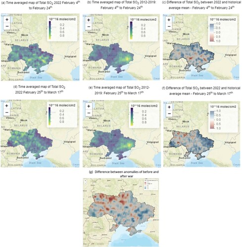
Figure 12a–f shows the spatial distribution of total column density SO₂ over Ukraine for three weeks before the conflict starts (2022 and historical mean) and three weeks after the conflict starts (2022 and historical mean). The SO₂ concentration in the atmosphere mostly varies drastically based on different emission sources and anthropogenic activities. In Ukraine, the major sources of SO₂ are coal mines, thermal heaters used in residential areas, and heavy industries (Savenets 2021). During the commencement of the war, from 4 February to 24 February in 2022 (Figure 12a), the SO₂ concentration is high in regions such as Donetsk, Dnipro, Odessa, Zaporizhzhia, and Kyiv. These are the most significant sources and impacted regions by SO₂ emissions. During this period, in 2022 the mean SO₂ concentration is 1.24 × 10¹⁶ molecules/cm² which is significantly higher at about 48% than the historical mean concentration, 0.84 × 10¹⁶ molecules/cm². The difference map shows that the vicinity of Kyiv, Donetsk, and Odessa regions have very high variations in 2022 compared to the historical trend (Figure 12c). After the war started the trend changed especially in the eastern regions of the country where the pollutant concentrations decreased (Figure 12f). Because most of the major sources of SO₂ emissions such as coal mining and other heavy industries that are distributed in the eastern regions are shut down. Kyiv and a few central parts of the country have a spike in SO₂ concentration. This unusual pattern may be resulted from the fuel combustion used for military vehicles and survival (Zalakeviciute et al. 2022).

Figure 12. Spatial distribution of total column density SO₂ over Ukraine. (a)–(b) are time-averaged maps of OMI total column density SO₂ from 4 February–24 February 2022, and 2012–2019. (c) is difference between the weekly average (before the conflict started) of 2022 and 2012–2019. (d)–(e) are time-averaged maps of OMI total column density SO₂ from 25 February–17 March 2022, and 2012–2019. (f) is difference between the weekly average (after the conflict started) of 2022 and 2012–2019. Figure 12 (g): Difference between anomalies before and after the war started.

Figure 13a–p shows the spatial pattern of SO₂ concentration over Kherson, Dnipro, Lviv, and Kharkiv before the war, the first week of the war, the second week of the war, and the third week of the war. Since the commencement of the war, the overall SO₂ concentration in the Kherson oblast is uneven across the region. The normalized mean concentration of SO₂ one week before the conflict, the first week of the conflict, the second week of the conflict, and the third week of the conflict in Kherson is 0.91, 0.93, 1.33, 0.33 × 10¹⁶ molecules/cm², respectively. During the first and second weeks of the war, Kherson had an active ground battle including an attack on the international airport in Kherson. In Dnipro, as shown in Figure 13h, from 11 March to 17 March 2022, the SO₂ concentration exceeds 4 × 10¹⁶ molecules/cm². During this period, the region was undergoing missile attacks that destroyed residential areas and airports. Over Lviv the SO₂ concentration is heterogeneous, varying drastically across the region. However, it is to be noted that during the initial invasion on 24 February, several missiles reached as far as Lviv. During this period, as shown in Figure 13i, there is a slight increase in SO₂ concentration over Lviv city. From Figure 13o, Kharkiv has a high SO₂ concentration on the second week of the war (4 March–10 March) exceeding 4 × 10¹⁶ molecules/cm². This period has the most intensified war activity with missiles attacking the residential areas and a nuclear research facility.

Figure 13. Spatial distribution of tropospheric SO₂ over Kherson, Dnipro, Lviv, and Kharkiv

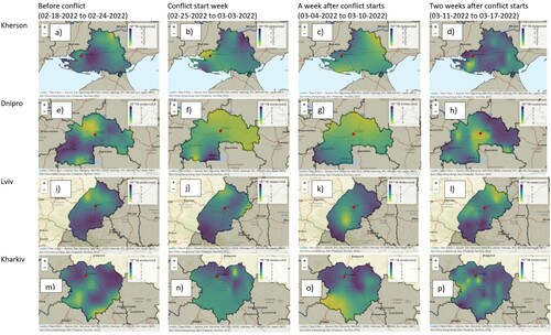
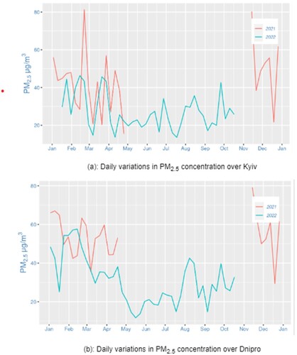
Figure 14. (a): Daily variations in PM_2.5 Concentartion over Kyiv; (b). Daily variations in PM_2.5 Concentartion over Dinpro.

3.4.3 PM_2.5 level three weeks before and after the war

This section discusses the PM_2.5 concentration in Ukraine, Kyiv, and Dnipro three weeks before and after the war. Prior to the war in Ukraine, the PM_2.5 concentration was 42.40 µg m⁻³, which decreased significantly to 38.7 µg m⁻³ after the conflict. A systematic study by (Zalakeviciute et al. 2022) analyzed the most polluted regions of Ukraine in 2018 and found that Kyiv accounted for only 3.2% of total air pollutant emissions, while Dnipro accounted for 24.5%. In Kyiv, the PM_2.5 concentration was 40 µg m⁻³ three weeks before the war, which was reduced to 25.95 µg m⁻³ after the conflict, indicating a 35.13% reduction. Dnipro’s PM_2.5 concentration was 54.09 µg m⁻³ before the war and 37.1 µg m⁻³ after the war. Figure 14a, and b illustrate the time series trend of PM_2.5 concentration in 2022 and 2021 in Kyiv and Dnipro. The gaps in the PM_2.5 time series are a result of insufficient data availability during certain periods. The trend shows a general decrease in PM_2.5 concentration in both cities in 2022 compared to 2021. Notably, the PM_2.5 concentration remained relatively low after the war started.

4. Conclusion and discussion

This paper investigated the air quality impacts of the COVID-19 pandemic and the Russian invasion on air quality in Ukraine by analyzing NO₂, SO₂, and O₃ data from OMI and TROPOMI sensors. The air quality data is processed using up-scaling and aggregation techniques to remove cloud contamination and subsequently ingested into an SDAP platform to visualize trends. Based on the experimental results and statistical analysis, it can be concluded that:

1. During the COVID-19 pandemic, the tropospheric NO₂ concentration was reduced by 2% in 2020 compared to the historical mean (2012–2019) before the lockdown and by 4% during the lockdown period. The reduction in anthropogenic emissions due to the strict quarantine policies might have attributed to the reduction in tropospheric NO₂ concentration in most of the industrialized zones of the country.

2. The total SO₂ column concentration was found to be reduced by 6% in 2020 before the lockdown compared to the same period in the historical mean (2012–2019) and reduced by 2.5% during the lockdown compared to the same period in the historical mean. High population density regions showed an increase in total column SO₂ during the lockdown, possibly due to the use of sulfur-containing fossil fuels for heating homes as people stayed indoors longer.

3. During the Russian invasion, the tropospheric NO₂ concentration between 25 February and 17 March is considerably reduced, with most of the eastern regions of the country showing a reduction in NO₂ concentration because of reduced human activities. Kharkiv, a major target for the Russian invasion and a heavily destroyed region had a considerably increased NO₂ concentration because of the war activities.

4. The total SO₂ column before the war is 48% higher than the historical mean. But after the war, the total SO₂ column was reduced throughout the country except for Kyiv and a few central regions of Ukraine.

To summarize, COVID-19 pandemic policies triggered a decrease in emissions from human activities, which led to lower levels of nitrogen dioxide in industrialized regions. However, the increase in the use of fossil fuels for heating during the lockdown period resulted in a rise in sulfur dioxide levels in densely populated areas. The war in Ukraine also impacted air quality, as there was a decrease in both nitrogen dioxide and sulfur dioxide levels. It is crucial to recognize that air pollution is connected to human health and the environment. Lower levels of NO₂ and SO₂ can result in better air quality and fewer respiratory issues, while elevated levels of these pollutants can have the opposite impact. Our knowledge about the effects of war on air quality is limited. Further research is necessary to understand the long-term implications of these events on air pollution and their impact on human health and the environment. A further detailed study is also needed to identify the correlation among war intensities, other related activities, specific air pollutants, and damages.

Data availability statement

OMI NO₂ data can be freely downloaded from the NASA GES DISC: https://disc.gsfc.nasa.gov/datasets/OMNO2d_003/summary; OMI SO2 can be freely downloaded from GES DISC: https://disc.gsfc.nasa.gov/datasets/OMSO2e_003/summary; OMI O3 can be freely downloaded from: https://disc.gsfc.nasa.gov/datasets/OMTO3e_003/summary. The Sentinel-5P Tropomi NO2 data can be freely downloaded from the European Space Agency Copernicus Open Access (https://scihub.copernicus.eu/) or the NASA GES DISC: https://disc.gsfc.nasa.gov/datasets/S5P_L2__NO2____1/summary.

Acknowledgements

We thank the NASA Goddard Earth Sciences (GES) Data and Information Services Center (DISC) for providing the Ozone Monitoring Instrument (OMI) NO₂, SO₂, and O₃. We thank the European Space Agency (ESA) for providing the TROPOspheric Monitoring Instrument (TROPOMI) NO₂. We would also like to thank the anonymous reviewers for their valuable comments.

Disclosure statement

No potential conflict of interest was reported by the author(s).

Additional information

Funding

This work is financially supported by NSF I/UCRC and START programs (1841520), NASA Goddard CISTO, and NASA AIST programs. This research was, in part, carried out at the Jet Propulsion Laboratory, California Institute of Technology, under a contract with the National Aeronautics and Space Administration (80NM0018D0004).

References

- AQICN. “Real-time Air Quality Index (AQI).” Accessed June 28, 2023. https://aqicn.org/.
- Åslund, Anders. 2020. “Responses to the COVID-19 Crisis in Russia, Ukraine, and Belarus.” Eurasian Geography and Economics 61 (4-5): 532–545. https://doi.org/10.1080/15387216.2020.1778499.
- Bhartia, Pawan K. 2005. “OMI/Aura Ozone (O3) Total Column 1-Orbit L2 Swath 13x24 km V003.” In Goddard Earth Sciences Data and Information Services Center (GES DISC), edited by Pawan K. Bhartia, 33–50. Greenbelt, MD, USA: Goddard Earth Sciences Data and Information Services Center (GES DISC).
- Bočková, Simona, Roman Bohovic, Matúš Hrnčiar, Mikuláš Muroň, Pavlína Filippovová, Martin Skalský, and Maksym Soroka. 2020. Air Pollution in Ukraine from Space. Edited by Jan Labohý: Arnika.
- Caiazzo, Fabio, Akshay Ashok, Ian A. Waitz, Steve H. L. Yim, and Steven R. H. Barrett. 2013. “Air Pollution and Early Deaths in the United States. Part I: Quantifying the Impact of Major Sectors in 2005.” Atmospheric Environment 79: 198–208. https://doi.org/10.1016/j.atmosenv.2013.05.081.
- Chandola, Varun, Arindam Banerjee, and Vipin Kumar. 2009. “Anomaly Detection: A Survey.” ACM Computing Surveys 41 (3): 1–58. https://doi.org/10.1145/1541880.1541882.
- Channell-Justice, Emily. 2023. “COVID-19 in Ukraine: Assessing the Government’s Response.” Ukrainian Research Institute at Harvard University, Accessed June 28, 2023. https://huri.harvard.edu/covid-19-ukraine-assessing-governments-response.
- D’Amato, G., K. C. Bergmann, L. Cecchi, I. Annesi-Maesano, A. Sanduzzi, G. Liccardi, C. Vitale, A. Stanziola, and M. D’Amato. 2014. “Climate Change and air Pollution.” Allergo Journal International 23 (1): 17–23. https://doi.org/10.1007/s40629-014-0003-7.
- Demchenko, Y., P. Grosso, C. de Laat, and P. Membrey. 2013. Addressing big Data Issues in Scientific Data Infrastructure. Paper Presented at the 2013 International Conference on Collaboration Technologies and Systems (CTS), 20–24 May 2013.
- Doyle, Gerry, Samuel Granados, Michael Ovaska, and Prasanta Kumar Dutta. 2023. “Weapons of the war in Ukraine.” Reuters, Accessed June 28, 2023. https://www.reuters.com/graphics/UKRAINE-CRISIS/WEAPONS/lbvgnzdnlpq/.
- El-Bawab, Nadine, and Martha Raddatz. 2023. “Lviv, Ukraine, hit with Missiles for 1st Time Since Russian Invasion.” ABCNews, Accessed June 29, 2023. https://abcnews.go.com/International/lviv-ukraine-hit-missiles-1st-time-russian-invasion/story?id = 83526019.
- Fenger, Jes. 1999. “Urban air Quality.” Atmospheric Environment 33 (29): 4877–4900. https://doi.org/10.1016/S1352-2310(99)00290-3.
- Filonchyk, Mikalai, Volha Hurynovich, Haowen Yan, Andrei Gusev, and Natallia Shpilevskaya. 2020. “Impact Assessment of COVID-19 on Variations of SO2, NO2, CO and AOD Over East China.” Aerosol and Air Quality Research 20 (7): 1530–1540. https://doi.org/10.4209/aaqr.2020.05.0226.
- George, Yasmeen, Shanika Karunasekera, Aaron Harwood, and Kwan Hui Lim. 2021. “Real-time Spatio-Temporal Event Detection on Geotagged Social Media.” Journal of Big Data 8 (91): 1–28. https://doi.org/10.1186/s40537-021-00482-2.
- Goldberg, Daniel L., Susan C. Anenberg, Gaige Hunter Kerr, Arash Mohegh, Zifeng Lu, and David G. Streets. 2021. “TROPOMI NO2 in the United States: A Detailed Look at the Annual Averages, Weekly Cycles, Effects of Temperature, and Correlation With Surface NO2 Concentrations.” Earth’s Future 9 (4): https://doi.org/10.1029/2020EF001665.
- Guille, Adrien, and Cécile Favre. 2015. “Event Detection, Tracking, and Visualization in Twitter: A Mention-Anomaly-Based Approach.” Social Network Analysis and Mining 5 (1): 1–18. https://doi.org/10.1007/s13278-015-0258-0.
- Guralnik, Valery, and Jaideep Srivastava. 1999. “Event Detection from Time Series Data.” In Proceedings of the Fifth ACM SIGKDD International Conference on Knowledge Discovery and Data Mining, 33–42, numpages=10. Association for Computing Machinery.
- Guttikunda, Sarath K., and Puja Jawahar. 2014. “Atmospheric Emissions and Pollution from the Coal-Fired Thermal Power Plants in India.” Atmospheric Environment 92: 449–460. https://doi.org/10.1016/j.atmosenv.2014.04.057.
- Hale, Thomas, Noam Angrist, Rafael Goldszmidt, Beatriz Kira, Anna Petherick, Toby Phillips, Samuel Webster, et al. 2021. “A Global Panel Database of Pandemic Policies (Oxford COVID-19 Government Response Tracker).” Nature Human Behaviour 5 (4): 529–538. https://doi.org/10.1038/s41562-021-01079-8.
- Huang, T., C. David, C. Oadia, J. T. Roberts, S. V. Kumar, P. Stackhouse, D. Borges, S. Baillarin, G. Blanchet, and P. Kettig. 2022. An Earth System Digital Twin for Flood Prediction and Analysis. Paper presented at the IGARSS 2022 - 2022 IEEE International Geoscience and Remote Sensing Symposium, 17–22 July 2022.
- Huang, Wei, Tianrui Li, Jia Liu, Peng Xie, Shengdong Du, and Fei Teng. 2021. “An Overview of air Quality Analysis by big Data Techniques: Monitoring, Forecasting, and Traceability.” Information Fusion 75: 28–40. https://doi.org/10.1016/j.inffus.2021.03.010.
- Isaifan, R. J. 2020. “The Dramatic Impact of Coronavirus Outbreak on air Quality: Has it Saved as Much as it has Killed so far?” Global Journal of Environmental Science and Management 6 (3): 275–288. https://doi.org/10.22034/gjesm.2020.03.01.
- Khurshudyan, Isabelle, and Miriam Berger. 2023. “Why Kharkiv, a City Known for its Poets, has Become a key Battleground in Ukraine.” The Washington Post, Accessed June 28, 2023. https://www.washingtonpost.com/world/2022/02/28/kharkiv-ukraine-russia-war-east/.
- Kinney, P. L. 2018. “Interactions of Climate Change, Air Pollution, and Human Health.” Current Environmental Health Reports 5 (1): 179–186. https://doi.org/10.1007/s40572-018-0188-x.
- Kisilevich, Slava, Florian Mansmann, Mirco Nanni, and Salvatore Rinzivillo. 2010. “Spatio-temporal Clustering.” In In Data Mining and Knowledge Discovery Handbook, edited by Oded Maimon, and Lior Rokach, 855–874. Boston, MA: Springer US.
- KNMI, Koninklijk Nederlands Meteorologisch Instituut. 2018. “Sentinel-5P TROPOMI Tropospheric NO2 1-Orbit L2 7 km x 3.5 km.” In Copernicus Sentinel Data Processed by ESA, edited by Beirle S, Richter A, and Sanders B, 23–50. Greenbelt, MD, USA: Goddard Earth Sciences Data and Information Services Center (GES DISC).
- Kovalenko, Pyotr, Anatoliy Rokochinskiy, Jerzy Jeznach, Roman Koptyuk, Pavlo Volk, Nataliіa Prykhodko, and Ruslan Tykhenko. 2019. “Evaluation of Climate Change in Ukrainian Part of Polissia Region and Ways of Adaptation to it.” Journal of Water and Land Development 41 (1): 77–82. https://doi.org/10.2478/jwld-2019-0030.
- Krotkov, Nickolay A, Lok N Lamsal, Sergey V Marchenko, Edward A Celarier, Eric J Bucsela, William H Swartz, Joanna Joiner, and OMI core team. 2019. “OMI/Aura NO2 Cloud-Screened Total and Tropospheric Column L3 Global Gridded 0.25 Degree x 0.25 Degree V3.” In, edited by Goddard Earth Sciences Data and Information Services Center (GES DISC), edited by Chance K., 13–36. Goddard Earth Sciences Data and Information Services Center (GES DISC).
- Kyrychko, Yuliya N, Konstantin B Blyuss, and Igor Brovchenko. 2020. “Mathematical Modelling of the Dynamics and Containment of COVID-19 in Ukraine.” Scientific Reports 10 (1): 1–11. https://doi.org/10.1038/s41598-019-56847-4.
- Li, Can, Joanna Joiner, Nickolay A. Krotkov, and Pawan K. Bhartia. 2013. “A Fast and Sensitive new Satellite SO2 Retrieval Algorithm Based on Principal Component Analysis: Application to the Ozone Monitoring Instrument.” Geophysical Research Letters 40 (23): 6314–6318. https://doi.org/10.1002/2013GL058134.
- Li, Can, Nickolay A. Krotkov, and Peter Leonard. 2020. “OMI/Aura Sulfur Dioxide (SO2) Total Column L3 1 day Best Pixel in 0.25 Degree x 0.25 Degree V3.” In Goddard Earth Sciences Data and Information Services Center (GES DISC), edited by Chance K., 49–58. Greenbelt, MD, USA: Goddard Earth Sciences Data and Information Services Center (GES DISC).
- Li, Yun, Moming Li, Megan Rice, and Chaowei Yang. 2022. “Impact of COVID-19 Containment and Closure Policies on Tropospheric Nitrogen Dioxide: A Global Perspective.” Environment International 158: 106887. https://doi.org/10.1016/j.envint.2021.106887.
- Liu, Qian, Jackson T Harris, Long S Chiu, Donglian Sun, Paul R Houser, Manzhu Yu, Daniel Q Duffy, Michael M Little, and Chaowei Yang. 2021a. “Spatiotemporal Impacts of COVID-19 on air Pollution in California, USA.” Science of The Total Environment 750: 141592. https://doi.org/10.1016/j.scitotenv.2020.141592.
- Liu, Q., A. S. Malarvizhi, W. Liu, H. Xu, J. T. Harris, J. Yang, D. Q. Duffy, et al. 2021b. “Spatiotemporal Changes in Global Nitrogen Dioxide Emission due to COVID-19 Mitigation Policies.” Science of The Total Environment 776: 146027. https://doi.org/10.1016/j.scitotenv.2021.146027.
- Liu, Qian, Dexuan Sha, Wei Liu, Paul Houser, Luyao Zhang, Ruizhi Hou, Hai Lan, et al. 2020. “Spatiotemporal Patterns of COVID-19 Impact on Human Activities and Environment in Mainland China Using Nighttime Light and Air Quality Data.” Remote Sensing 12 (10): 1576. https://doi.org/10.3390/rs12101576.
- Liu, Qian, Anusha Srirenganathanmalarvizhi, Katherine Howell, and Chaowei Yang. 2022. “Tropospheric Nitrogen Dioxide Increases Past Pre-Pandemic Levels Due to Economic Reopening in India.” Frontiers in Environmental Science 10, https://doi.org/10.3389/fenvs.2022.962891.
- Longley, Paul A, Michael F. Goodchild, David J. Maguire, and David W. Rhind. 2015. Geographic Information Science and Systems. Hoboken, NJ, USA: John Wiley & Sons.
- Magazzino, C., M. Mele, and N. Schneider. 2020. “The Relationship Between air Pollution and COVID-19-Related Deaths: An Application to Three French Cities.” Applied Energy 279: 115835. https://doi.org/10.1016/j.apenergy.2020.115835.
- Medioni, G., I. Cohen, F. Bremond, S. Hongeng, and R. Nevatia. 2001. “Event Detection and Analysis from Video Streams.” IEEE Transactions on Pattern Analysis and Machine Intelligence 23 (8): 873–889. https://doi.org/10.1109/34.946990.
- Nádudvari, Ádám, Anna Abramowicz, Monika Fabiańska, Magdalena Misz-Kennan, and Justyna Ciesielczuk. 2021. “Classification of Fires in Coal Waste Dumps Based on Landsat, Aster Thermal Bands and Thermal Camera in Polish and Ukrainian Mining Regions.” International Journal of Coal Science & Technology 8 (3): 441–456. https://doi.org/10.1007/s40789-020-00375-4.
- Nordlund, Göran. 2000. “Emissions, air Quality and Acidifying Deposition.” In Forest Condition in a Changing Environment: The Finnish Case, edited by Eino Mälkönen, 49–59. Dordrecht: Springer Netherlands.
- Popov, O., A. Iatsyshyn, V. Kovach, V. Artemchuk, I. Kameneva, D. Taraduda, V. Sobyna, D. Sokolov, M. Dement, and T. Yatsyshyn. 2020. “Risk Assessment for the Population of Kyiv, Ukraine as a Result of Atmospheric Air Pollution.” Journal of Health and Pollution 10 (25): 200303. https://doi.org/10.5696/2156-9614-10.25.200303.
- Pravda. 2023. “From September 23, all Regions of Ukraine Have a “Yellow” Level of Epidemic Safety.” Ukrainska Pravda, Accessed June 28, 2023. https://www.pravda.com.ua/news/2021/09/21/7307872/.
- Protopsaltis, C. 2012. “WIT Transactions on Ecology and The Environment.” WIT Transactions on Ecology and the Environment 157: 93–98. https://doi.org/10.2495/AIR120091.
- Rawtani, D., G. Gupta, N. Khatri, P. K. Rao, and C. M. Hussain. 2022. “Environmental Damages due to war in Ukraine: A Perspective.” Science of The Total Environment 850: 157932. https://doi.org/10.1016/j.scitotenv.2022.157932.
- Rodríguez-Urrego, D., and L. Rodríguez-Urrego. 2020. “Air Quality During the COVID-19: Pm2.5 Analysis in the 50 Most Polluted Capital Cities in the World.” Environmental Pollution 266 (Pt 1): 115042. https://doi.org/10.1016/j.envpol.2020.115042.
- Rogalski, Leszek, Lech Smoczynski, Sławomir Krzebietke, Leszek Lenart, and Ewa Mackiewicz-Walec. 2014. “Changes in Sulphur Dioxide Concentrations in the Atmospheric air Assessed During Short-Term Measurements in the Vicinity of Olsztyn, Poland.” Journal of Elementology 19: 735–748. https://doi.org/10.5601/jelem.2014.19.2.634.
- Savenets, Mykhailo. 2021. “Air Pollution in Ukraine: A View from the Sentinel-5P Satellite.” IDŐJÁRÁS/QUARTERLY JOURNAL OF THE HUNGARIAN METEOROLOGICAL SERVICE 125 (2): 271–290. https://doi.org/10.28974/idojaras.2021.2.6.
- Sergeeva, Anastasiya, Inga Zinicovscaia, Konstantin Vergel, Nikita Yushin, and Mira Aničić Urošević. 2021. “Sources and Consequences of Groundwater Contamination.” Archives of Environmental Contamination and Toxicology 80 (1): 1–10. https://doi.org/10.1007/s00244-020-00805-z.
- Sha, Dexuan, Yi Liu, Qian Liu, Yun Li, Yifei Tian, Fayez Beaini, Cheng Zhong, et al. 2021. “A Spatiotemporal Data Collection of Viral Cases for COVID-19 Rapid Response.” Big Earth Data 5 (1): 90–111. https://doi.org/10.1080/20964471.2020.1844934.
- Shin, Daegeun, Seungjoo Song, Sang-Boom Ryoo, and Sang-Sam Lee. 2020. “Variations in Ozone Concentration Over the Mid-Latitude Region Revealed by Ozonesonde Observations in Pohang, South Korea.” Atmosphere 11 (7): 746. https://doi.org/10.3390/atmos11070746.
- Souto, Gustavo, and Thomas Liebig. 2016. “On Event Detection from Spatial Time Series for Urban Traffic Applications.” In In Solving Large Scale Learning Tasks. Challenges and Algorithms: Essays Dedicated to Katharina Morik on the Occasion of Her 60th Birthday, edited by Stefan Michaelis, Nico Piatkowski, and Marco Stolpe, 221–233. Cham: Springer International Publishing.
- Torkmahalleh, M. A., Z. Akhmetvaliyeva, A. Darvishi Omran, F. Darvish Omran, M. Kazemitabar, M. Naseri, M. Naseri, et al. 2021. “Global air quality and COVID-19 pandemic: do we breathe cleaner air?”.
- Wang, Chunjiao, Ting Wang, Pucai Wang, and Vadim Rakitin. 2020. “Comparison and Validation of TROPOMI and OMI NO2 Observations Over China.” Atmosphere 11 (6): 636. https://doi.org/10.3390/atmos11060636.
- Wei, Jing, Song Liu, Zhanqing Li, Cheng Liu, Kai Qin, Xiong Liu, Rachel T. Pinker, et al. 2022. “Ground-Level NO2 Surveillance from Space Across China for High Resolution Using Interpretable Spatiotemporally Weighted Artificial Intelligence.” Environmental Science & Technology 56 (14): 9988–9998. https://doi.org/10.1021/acs.est.2c03834.
- WHO. 2023. “Billions of People Still Breathe Unhealthy air: New WHO Data.” World Health Organization, Accessed June 25, 2023. https://www.who.int/news/item/04-04-2022-billions-of-people-still-breathe-unhealthy-air-new-who-data.
- World Nuclear Association. 2023. “Nuclear Power in Ukraine.” Accessed June 28, 2023. https://world-nuclear.org/information-library/country-profiles/countries-t-z/ukraine.aspx.
- Wu, X., R. C. Nethery, B. M. Sabath, D. Braun, and F. Dominici. 2020. “Exposure to air pollution and COVID-19 mortality in the United States: A nationwide cross-sectional study.” medRxiv. https://doi.org/10.1101/2020.04.05.20054502.
- Yang, Chaowei, Qunying Huang, Zhenlong Li, Kai Liu, and Fei Hu. 2016a. “Big Data and Cloud Computing: Innovation Opportunities and Challenges.” International Journal of Digital Earth 10 (1): 13–53. https://doi.org/10.1080/17538947.2016.1239771.
- Yang, Chaowei, Dexuan Sha, Qian Liu, Yun Li, Hai Lan, Weihe Wendy Guan, Tao Hu, et al. 2020. “Taking the Pulse of COVID-19: A Spatiotemporal Perspective.” International Journal of Digital Earth 13 (10): 1186–1211. https://doi.org/10.1080/17538947.2020.1809723.
- Yang, Chaowei, Manzhu Yu, Fei Hu, Yongyao Jiang, and Yun Li. 2016b. “Utilizing Cloud Computing to Address Big Geospatial Data Challenges.” Computers, Environment and Urban Systems 61: 120–128. https://doi.org/10.1016/j.compenvurbsys.2016.10.010.
- Yin, Jie, Derek Hao Hu, and Qiang Yang. 2009. “Spatio-temporal Event Detection Using Dynamic Conditional Random Fields.” Paper Presented at the Twenty-First International Joint Conference on Artificial Intelligence.
- Yu, Manzhu, Myra Bambacus, Guido Cervone, Keith Clarke, Daniel Duffy, Qunying Huang, Jing Li, et al. 2020. “Spatiotemporal Event Detection: A Review.” International Journal of Digital Earth 13 (12): 1339–1365. https://doi.org/10.1080/17538947.2020.1738569.
- Zalakeviciute, Rasa, Danilo Mejia, Hermel Alvarez, Xavier Bermeo, Santiago Bonilla-Bedoya, Yves Rybarczyk, and Brian Lamb. 2022. “War Impact on Air Quality in Ukraine.” Sustainability 14 (21): 13832. https://doi.org/10.3390/su142113832.
- Zvyagintsev, A. M., O. B. Blum, A. A. Glazkova, S. N. Kotel’nikov, I. N. Kuznetsova, V. A. Lapchenko, E. A. Lezina, et al. 2011. “Anomalies of Trace Gases in the air of the European Part of Russia and Ukraine in Summer 2010.” Atmospheric and Oceanic Optics 24 (6): 536–542. https://doi.org/10.1134/S1024856011060145.