Ice bottom evolution derived from thermistor string-based ice mass balance buoy observations

ABSTRACT

Digital information on sea ice extent, thickness, volume, and distribution is crucial for understanding Earth's climate system. The Snow and Ice Mass Balance Apparatus (SIMBA) is used to determine snow and ice temperatures in Arctic, Antarctic, ice-covered seas, and boreal lakes. Snow depth and ice thickness are derived from SIMBA temperature regimes (SIMBA_ET and SIMBA_HT). In warm conditions, SIMBA_ET temperature-based ice thickness may have errors due to the isothermal vertical profile. SIMBA_HT provides a visible ice-bottom interface for manual quantification. We propose an unmanned approach, combining neural networks, wavelet analysis, and Kalman filtering (NWK), to mathematically establish NWK and retrieve ice bottoms from various SIMBA_HT datasets. In the Arctic, NWK-derived total thickness showed a bias range of −5.64 cm to 4.01 cm and a correlation coefficient of 95%−99%. For Baltic Sea ice, values ranged from 1.31 cm to 2.41 cm (88%−98% correlation), and for boreal lake ice, −0.7 cm to 2.6 cm (75%−83% correlation). During ice growth, thermal equilibrium, and melting, the bias varied from −3.93 cm to 2.37 cm, −1.92 cm to 0.04 cm, and −4.90 cm to 3.96 cm, with correlation coefficients of 76%−99%. These results demonstrate NWK's robustness in retrieving ice bottom evolution in different water environments.

KEYWORDS:

• Sea ice thickness
• lake ice thickness
• ice-bottom evolution
• nonlinear filtering

1. Introduction

Unlike other materials, water has three phases that exist simultaneously in nature. Of these three phases, ice constitutes the smallest proportion, yet it represents an essential component of Earth’s cryosphere system. The largest portion of ice exists in the polar region. Polar amplification (known as air temperature increases faster in polar regions than in the rest of the world) extensively alters the phase change of water and further impacts global climate (Feldl and Merlis 2021; Holland and Landrum 2021; Smith et al. 2019). A fundamental topic that has been investigated for decades is the snow and ice mass balance for natural water bodies (Lei et al. 2022; Wagner and Frame 2015; Wever et al. 2021). Quantification of the ice thickness (IT) evolution is the main challenge in understanding the ice mass balance because this process involves comprehensive air–ice-water interactions that impact the climate. This topic has been tackled across a large spatial and temporal scale by investigating sea ice thickness (SIT) in the Arctic Ocean (Johannessen et al. 2022; Lang, Yang, and Kaas 2017; Rantanen et al. 2022). On a local scale, the research objective is often targeted at the evolution of air-snow-ice-water interactions (Kwok 2018; Provost et al. 2017), among which the thermodynamic processes of freezing and ablation of the ice thickness are of particular interest because they play key roles in determining the ice thickness.

SIT and IT changes in the polar ocean, seasonal ice-covered seas and boreal lakes further affect the light and heat distribution in the atmosphere, ice, and aquatic environment below the ice, with considerable physical and biological implications (Wang et al. 2018). Lake IT thinning results in a shorter ice season in the Northern Hemisphere (Lopez, Hewitt, and Sharma 2019). Peaks and declines in spring phytoplankton population growth (Weyhenmeyer 2001) and water quality (Weyhenmeyer 2009) are influenced by lake ice breakup variations. These changes can influence lake ecosystem conditions in ways that are difficult to predict. Thus, timely and accurate IT measurements profoundly impact our understanding of air-snow-ice-water interactions, allowing us to predict climate change trends (Filazzola et al. 2020). In addition, accurate SIT (IT) information services are vital for marine navigation, offshore industries, and local communities whose livelihoods, such as winter fishing, transportation, and recreational activities, involve interaction with ice (Lei et al. 2015). Thinning IT increases the heat flux from water to the atmosphere, increasing precipitation, and enhancing the interaction between snow and ice (Leppäranta 1983). Thinner ice facilitates ease of navigation and offshore activities in the Arctic, further increasing the need for marine and weather forecasts and services.

Remote-sensing technology development has enabled large-scale sea ice monitoring, particularly over the past four decades. Consequently, this has resulted in the production of satellite-based SIT products for the Arctic Ocean (Kwok and Rothrock 2009; Miller, Cresswell, and Laxon 2003; Sallila et al. 2019). However, these products depend on several parameters, such as snow depth, snow density, and sea ice density. The variability of these parameters may generate uncertainties in the SIT retrieval (Lei et al. 2021; Zygmuntowska et al. 2014). Therefore, the validation and improvement of satellite-based IT products require in situ observations, in particular, the snow depth and ice thickness.

Unmanned snow and ice mass balance buoys (IMB) are widely used to obtain snow and IT information in polar regions. IMBs, designed by the Cold Regions Research and Engineering Laboratory (CRREL), are used to determine snow, ITs, and vertical temperature profiles in combination with acoustic sensors and a thermistor chain (Richter-Menge et al. 2006; Zygmuntowska et al. 2014). The thermistor string-based snow and ice mass balance apparatus (SIMBAs), designed by the Scottish Association for Marine Science Research Services Ltd., Scotland (Jackson et al. 2013), has been used to study polar oceans (Koo et al. 2021; Lei et al. 2022) and ice in lakes and rivers (Cheng et al. 2020; Cheng et al. 2022) because of its cost-cutting design, easy deployment, and economic viability. The air-snow-ice-water temperature patterns revealed by environmental temperature, namely SIMBA_ET, were used to derive snow depth and IT, especially during cold conditions, which yielded reliable results (e.g. Liao et al. 2019; Zuo, Dou, and Lei 2018). SIMBA heating, namely SIMBA-HT, serves as a complementary dataset and can be solely used to cross-verify the SIMBA-ET-derived interfaces (Liao et al. 2019). Applying SIMBA to monitor IT has expanded. However, few automated algorithms have been developed to accurately identify the evolution of ice-bottoms. The manual identification of interfaces from SIMBA_ET still remains a prevalent practical approach. SIMBA_HT often yields a visual interface at the ice-bottom owing to the different heat capacities and conductivities of ice and water. However, unmanned quantification of such interface positions from the SIMBA_HT time series is not trivial. The challenge here is to extract and quantify the ice-bottom position from the visible ice-water interface in SIMBA_HT data using a mathematical algorithm-based approach, which adequately adheres to the findability, accessibility, interoperability, and reusability (FAIR) principle (Wilkinson et al. 2016).

In this study, we propose a new approach, NWK, which consists of a) artificial neural networks (NEN), b) wavelet filtering analyzes (WAA), and c) Kalman filtering (KAF) to automatically identify the ice-water interface from the SIMBA_HT data. This study aims to accurately determine the position of a moving interface from the spatiotemporal temperature regime observed in ice and water. This issue can also be categorized as an edge detection (ED) problem. Unlike the identification of sea ice/open water edges in the Pan-Arctic domain, our focus was on identifying a continuous interface evolution governed by thermodynamic physics and energy conservation law.

The SIMBA data used in this study are described in Section 2. The NWK approach is presented in Section 3, followed by a discussion of the results in Section 4. Finally, the conclusions are presented in Section 5.

2. Data

2.1. SIMBA data

Two types of temperatures were measured using the SIMBA buoy, namely SIMBA_ET and SIMBA_HT. The temperatures of air, snow, ice, and water where the SIMBA thermistor sensors were placed were termed ‘SIMBA_ET’. The temperature readings obtained after subjecting each thermistor sensor to an identical amount of heat were named SIMBA_HT. The amount of heat was controlled by the duration of heating, often configured as 60 and 120 s, immediately following the SIMBA_ET measurement. SIMBA_ET and SIMBA_HT were measured four times and once daily, respectively. By subtracting SIMBA_ET, we obtain SIMBA_HT (1) and SIMBA_HT (2), representing the changes in air, snow, ice, and water temperatures during the 60 and 120 s heating periods, respectively. We can also calculate the SIMBA_HT heating rate, such as [SIMBA_HT (2) - SIMBA_HT (1)] / 60. The minimum temperature change that the SIMBA sensor could identify was ±0.0625 °C. The SIMBA_HT regime is a quantitative measurement of how air, snow, ice, and water react to heat diffusivity during heating cycles. In this study, we used SIMBA_HT data to identify the evolution of the ice-bottom.

2.2. SIMBA buoy observations

SIMBA data were obtained from the Arctic Ocean, Lake Orajärvi, and the Baltic Sea (Table 1). These sites were selected to represent different environments in ice-water interactions. For Arctic conditions, SIMBAs were deployed on thick-level ice floes away from open leads and ice cracks. This ensures that SIMBAs operate for a sufficiently long period, often lasting from a few months to more than a year. The SIMBAs were deployed at fixed locations in Lake Orajärvi and the Baltic Sea during the entire observation period, covering a large portion of the ice season (3-4 months) Figure 1.

Figure 1. Deployment status of Snow and Ice Mass Balance Apparatus (SIMBA) and positions during deployment. (a) The Arctic Ocean, photo by Anne Bublitz (AWI), (b) the boreal Lake Orajärvi, photo by Bin Cheng (FMI), and (c) the Baltic Sea, photo by Pekka Kosloff (FMI). The yellow box represents the SIMBA’s main case. The ice thermistor string was placed vertically through the air-snow-ice-water interface. d) SIMBA buoy positions (blue dot: Lake Orajärvi; red dot: the Baltic Sea).

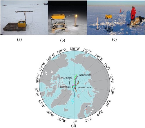
Table 1. Snow and Ice Mass Balance Apparatus (SIMBA) deployment status for various natural water environments.

Name (ID)	Location	Starting date	Thickness (m)			Sensor Interface Positions (SIPs)				Ending date
			Hi	Hs	Hf	Air/Snow	Sea Level	Snow/Ice	Ice bottom
FMI0403*	Arctic Ocean	18/08/2018	1.26	0.05	0.11	43	45	51	108	12/05/2019
FMI0505**		17/09/2018	2.11	0.03	0.47	21	21	44	126	19/09/2019
FMI0504R**		11/09/2018	2.62	0.00	0.80	23	23	63	154	24/09/2019
PRIC0903+		11/10/2018	1.74	0.14	0.24	28	35	47	122	21/04/2019
FMI0509+		08/10/2019	1.57	0.10	0.09	18	23	27	101	19/04/2020
FMI17R++		21/08/2018	1.55	0.06	0.25	42	45	58	123	28/12/2018
FMI0507++		23/08/2018	1.81	0.07	0.25	44	47	59	138	27/12/2018
FMI17	Baltic Sea	14/01/2017	0.42	0.01	−0.02	168	167	168	189	25/03/2017
FMI13		26/01/2019	0.43	0.14	0.00	90	90	90	112	01/04/2019
FMI09	Lake Orajärvi	14/12/2014	0.30	0.19	−0.03	145	146	150	163	05/02/2015
FMI0402		15/12/2016	0.31	0.08	−0.01	108	109	110	136	26/03/2017

* CHINARE2018; ** NABOS2018;+MOSAiC2019; ++ CAATEX2018 (SIPs is the initial different interface positions recorded with the SIMBA sensor number, including the air/snow interface, sea level position, snow/ice interface, and ice-bottom interface. Hi is the height of the ice, Hs is the height of the snow, and Hf is the height of the freeboard).

2.3. SIMBA_HT data characteristics

The range of variation of SIMBA_HT was much smaller than that of SIMBA_ET. For the air temperature sensor, heating can cause a temperature change of 1.0-3.0 ${}^{\circ }C$, depending on the season and heating time interval. For instance, temperature rises of about 0.75 ${}^{\circ }C$ and 1.5 ${}^{\circ }C$ can be reached after 60 and 120 s heating cycles, respectively. In ice and water, the temperature rise was less than 1.0 ${}^{\circ }C$ (Jackson et al. 2013). Based on this principle, SIMBA_HT records the temperature variation of different environmental media after providing the same amount of energy throughout the heating cycle for each sensor, resulting in visible interfaces.

However, in practice, the visibility of the ice-bottom interface can occasionally be compromised by various noise signals arising from the inevitable fluctuations in the surrounding environment near the sensors. Consequently, the original SIMBA_HT time series may exhibit striped disturbances (Figure 2b). Furthermore, in a snowpack, particle bubbles and pores have an impact on the temperature variations around the sensor after heating. In air, sensor freezing, solar radiation, surface roughness at the air-snow interface, and other factors contribute to the noise present in SIMBA_HT data. However, due to the relatively slow and stable freezing process of ice at the bottom, the ice-water interface remains visible and can be extracted from the noise-striped field.

Figure 2. (a) Example vertical SIMBA_HT (red) and SIMBA_ET (blue) profiles observed on 14:01:12, 12 November 2018 by SIMBA FMI0504R. (b) Part of the raw SIMBA_HT time series of FMI0504R ranged from ice-freeboard to the water, from mid-January to June.

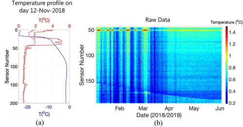
In addition to the microphase characteristic-induced noise mentioned above, the SIMBA_HT data were also affected by several heating factors, such as the small value of pulse heating, the short duration of the heating cycle, and the change in the ice heat capacity caused by the change in the internal structure of the ice and brine content. These effects caused by heating and the microphase characteristics complicate pinpointing the ice-bottom interface, which one can do solely by monitoring the freezing temperature of the water near the ice-bottom. In addition, the increased temperature values caused by the heating cycle complicate directly identifying the ice-bottom by checking the vertical temperature gradients, as can be done with SIMBA_ET, because the temperature profiles of SIMBA_HT are substantially variable at different moments (Jackson et al. 2013). Moreover, the SIMBA_HT time series was influenced by environmental perturbations, which manifested as local streak properties over time. For example, the original SIMBA_HT time series (Figure 2b) shows striped perturbations when focusing on sensors ranging from the snow-ice interface to the water.

3. Methods

To detect the ice-bottom interfaces from SIMBA_HT, we first denoised the SIMBA_HT data using an artificial neural network (Guan, Lai, and Xiong 2019). We then defined a fixed sensor number range, denoted as $\phi$, to focus on SIMBA_HT near the bottom of the ice. We captured the support points of the ice-bottom interface using wavelet filtering and obtained the signal points of the ice-bottom interface by applying a threshold truncation to the vertical SIMBA_HT gradients. Utilizing these support points, we introduced a sensor range and found the ice-bottom interface in this range using the Kalman filter method. In this section, we consider the SIMBA_HT time series collected by the buoy FMI0504R as an example to illustrate the proposed method.

3.1. Data processing

First, the original SIMBA_HT data were rearranged into a data matrix. The $i$th column of the data matrix corresponds to the vertical SIMBA_HT data recorded at the $i$th time point. This operation preserves the temporal continuity and marginal spatial distribution of the SIMBA_HT data while providing an opportunity to denoise SIMBA_HT using existing image processing methods.

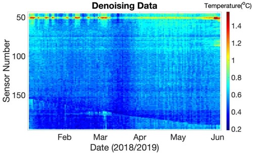
Specifically, our method uses a streak-denoising wavelet deep neural network (SNRWDNN) (Guan, Lai, and Xiong 2019) to remove stripe noise from the raw SIMBA_HT time series. The SNRWDNN consists of three subprocesses: Haar discrete wavelet transform (HDWT), wavelet coefficient prediction neural network, and inverse Haar discrete wavelet transform (IHDWT). The HDWT is used to obtain the sub-band coefficients that characterize the stripe noise. These coefficients were then concatenated as input tensors and fed into the prediction network to evaluate the strip components. The prediction network consists of M + 1 convolutional layers with residual connections, where the outputs of the convolutional layers are fed into Rectified Linear Unit (ReLU) activation functions. The prediction network also includes a skip connection that adds the network input to its output. Finally, the IHDWT was used to evaluate the coefficients to reconstruct the de-striped results in the spatial domain. As shown in Figure 3, most of the stripe noise in the raw SIMBA_HT time series was removed by the SNRWDNN. For convenience, we termed the denoised SIMBA_HT time series extended SIMBA_HT as follows.

Figure 3. The part of denoised extended SIMBA_HT. Strip disturbance is removed by the streak-denoising wavelet deep neural network (SNRWDNN) model.

As the temperature differences in SIMBA_HT between the upper and lower sides of the ice-bottom are minute, traditional edge detection methods such as the wavelet method (Shih and Tseng 2005), Canny operator (Canny 1983), and Prewitt operator (Chaudhuri and Chanda 1984), often lead to significant errors in extracting the ice-bottom from the extended SIMBA_HT. Fortunately, by truncating the absolute values of the vertical temperature gradients, we can find a set of points that includes the actual ice-bottom interface. These points are termed ‘ice-bottom potential points (IBPPs).’ Based on the continuity of the ice-bottom interface and the correlation between the credible part of the IBPPs and the ice-bottom interface, we can obtain ice-bottom signal points (IBSPs) and apply the Kalman filter method to provide an actual ice-bottom interface. This allows us to extract IBPPs from SIMBA_HT data. The following subsection describes how we obtained the IBPPs and IBSPs.

3.2. Locating IBPPs and IBSPs

SIMBA_HT records the heating temperature data at different depths, including in air, snow, ice, and water. In this study, our goal was to detect the ice-bottom interface (the location of the ice–water interface); therefore, we were interested in the SIMBA_HT data near this location. For this reason, we set a sensor number range $\phi$ for SIMBA. This sensor number range $\phi$ indicates the part of the sensors located in the ice and water and helps to remove the SIMBA_HT unrelated to the ice-bottom. Based on $\phi$, we will further introduce a dynamic sensor range $\mathrm{\Omega }\subset \phi$ by translating the results of the RTA algorithm up and down. The dynamic sensor range $\mathrm{\Omega }$ will help us reduce the sensors in $\phi$ to search the ice-bottom at different moments. Finally, by thresholding the absolute value of the vertical gradient of temperature within $\mathrm{\Omega }$ and using a certain interpolation technique, we can find the set of IBPPs. Feeding IBSPs into the Kalman filter led to an estimation of the actual ice-bottom interface. Next, we will present how to determine the rectangular $\phi$, dynamic sensor range $\mathrm{\Omega }$, IBPPs, and IBSPs.

In particular, the range $\phi$ is evaluated by the RTA algorithm based on SIMBA_ET. The RTA results provided the highest and lowest sensor indices for the ice-bottom. These indices comprise the upper and lower boundaries of the range $\phi$. Although the RTA algorithm cannot use SIMBA_HT to calculate the ice-bottom interface, the results remain reliable for ice growth and thermal equilibrium periods. Thus, the highest and lowest sensor indexes of the ice-bottom obtained from RTA are also significant to determine the range $\phi$ such that SIMBA_HT data near the ice-bottom interface are included in $\phi$.

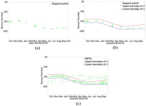
Next, we explain how we determined the dynamic sensor range $\mathrm{\Omega }$. We observed that the ice-bottom curve always passed through the points generated by wavelet filtering. We refer to these points as support points (Figure 4a). Therefore, we require that $\mathrm{\Omega }$ contains all support points during the SIMBA buoy work cycle. We find these support points in the following way.

Figure 4. a) The distribution of support points for the time series collected by the buoy FMI0504R. These green points are the coordinates of support points in $P_{sub}$; b) Two boundaries of the dynamic sensor range $\mathrm{\Omega }$ and support points of $P_{sub}$. The red curve is the upper boundary, and the blue curve is the lower boundary; and c) The upper and lower boundaries of the dynamic sensor range $\mathrm{\Omega }$ and ice-bottom potential points (IBPPS).

We denote the extended SIMBA_HT as a data matrix $T_{M\ast N}$, where $M$ is the number of sensors and $N$ is the number of sampling moments. Let $t_{i,j}$ be the element of $T_{M\ast N}$ in the $i$th row and $j$th column, that is, $t_{i,j}$ represents the data value recorded by the $i$th sensor of the SIMBA buoy at moment $j$. Suppose that there is one vertical SIMBA_HT, data $T_j$ recorded at moment $j$, that is, $T_j=(t_{1j},t_{2j},\dots ,t_{Mj}{)}^T$. By treating $T_j$ as a one-dimensional vector, we obtain a new temperature data vector $T_j^{\mathrm{\prime }}$ by the following transformation: (1) $T_J^{\mathrm{\prime }}=W^{T}XW{T}_j,$(1) where $W$ is an $M\ast M$ Haar wavelet transform matrix, $X$ is an $M\ast M$ truncation matrix that obtains the wavelet coefficients of the fourth layer after the 5-layer wavelet transform, and $W^T$ is an inverse Haar wavelet transform matrix. Applying the above operation to series $\{T_j|j=1,2,3,\dots ,N\}$, we obtain a new one-dimensional temperature data time series $\{T_j^{\mathrm{\prime }}|j=1,2,3,\dots N\}$, and denote it as a new data matrix $T_{M\ast N}^{\mathrm{\prime }}=\left(T_1^{\mathrm{\prime }},T_2^{\mathrm{\prime }},\dots ,T_N^{\mathrm{\prime }}\right)$. We denote the $i$th row and $j$th column elements of $T_{M\ast N}^{\mathrm{\prime }}$ as $t_j^{,}$. We maintain the indexes of the elements in $T_{M\ast N}^{\mathrm{\prime }}$, which satisfy $0.0625{}^{\circ }C<\left|t_{i,j}^{,}\right|<0.7{}^{\circ }C$ and $\left(i,j\right)\in \phi$. These indices are the coordinates of the support points, (2) $P_{sup}=\left\{\right(i,j\left)\right|0.0625{}^{\circ }C<\left|t_{i,j}^{,}\right|<{0.7}^{\circ }C,\left(i,j\right)\in \phi \},$(2) where $P_{sup}$ is the index set of all support points in the matrix $T_{M\ast N}^{,}$. The reason for using condition $0.0625{}^{\circ }C<\left|t_{i,j}^{,}\right|<0.7{}^{\circ }C$ is that using condition $\left|t_{i,j}^{,}\right|\le 0.0625{}^{\circ }C$ will cause $P_{sup}$ to contain too many fake support points. However, if $\left|t_{i,j}^{,}\right|>0.7{}^{\circ }C$, the elements in set $P_{sup}$ are too few to utilize. A range of $0.0625{}^{\circ }\mathrm{C}<\left|t_{i,j}^{,}\right|<0.7{}^{\circ }\mathrm{C}$ retains the appropriate correlation with the location of the ice-bottom interface.

Combining $P_{sup}$ and the outputs of the RTA algorithm, we obtain the dynamic sensor range as follows: During the ice growth seasons and thermal equilibrium periods, the outputs of the RTA algorithm were regarded as reference curves. We obtained the limitation curves of the ice-bottom with respect to the ice-melting rate during the melting season. Furthermore, we obtained the upper and lower range boundaries of range $\mathrm{\Omega }$ at different moments by translating the reference and limitation curves. To ensure $\mathrm{\Omega }$ is reliable for ice-bottom detection, we require the translation of the reference and limitation curves to guarantee that all support points in $P_{sup}$ are included in $\mathrm{\Omega }$ (Figure 4b). In the experiments, we assumed that the ice-melting rate ranges of 0-9 cm/month during the ice-melting periods.

The next step is to find the IBPPs in the range $\mathrm{\Omega }$. Let $P$ be the point set of the IBPPs satisfying. (3) $P=\{\left(i,j\right)|\left(i,j\right)\in \mathrm{\Omega },0.0625{}^{\circ }C\le \left|t_{ij}-t_{\left(i+1\right)j}\right|\le {0.125}^{\circ }C\}$(3) where $t_{ij}$ represents the SIMBA_HT data recorded by the $i$th sensor at time $j$. We chose $0.125{}^{\circ }C$ as the threshold value because we found that the absolute values of vertical gradients of SIMBA_HT near the ice-bottom are almost less than $0.5$ ${}^{\circ }C$ and more than $0.0{}^{\circ }C$, but the minimum identification temperature of SIMBA sensors is $0.0625{}^{\circ }C$. Smaller threshold values cause set $P$ to include too many points. A larger threshold value makes the points too sparse to identify the IBSPs. Hence, we used the conditions shown in Equation (3(3) $P=\{\left(i,j\right)|\left(i,j\right)\in \mathrm{\Omega },0.0625{}^{\circ }C\le \left|t_{ij}-t_{\left(i+1\right)j}\right|\le {0.125}^{\circ }C\}$(3) ) (Figure 4c).

Based on point set $P$, we can determine the IBSPs using the following two steps: First, we consider the moments with IBPPs in point set $P$ first. In this case, we compute the average of the indices of the IBPPs simultaneously. For instance, if there are n IBPPs $\left(n\ge 1\right)$ $q_1=\left(i_1,j\right),q_2=\left(i_2,j\right),\dots ,q_n=\left(i_n,j\right)$ at the moment $j$ in $P$, we let the IBSP at the moment j be $h_j=\left(\frac{{\sum }_{k=1}^n{i}_k}{n}\right)\ast 2cm$. In the second step, we consider moments without any IBPP in $P$. We applied a linear interpolation to the IBSPs $\left\{h_j\right\}$ obtained in the first step. For example, suppose that there are IBSPs $h_j,$ and $h_{j+m+1}$ at moments $j$ and $j+m+1$, and that there is no IBPP at moments $j+1$, $j+2,\dots ,\mathrm{a}\mathrm{n}\mathrm{d}j+m$ in $P$. We set IBSPs $h_{j+k}={\displaystyle \frac{k\ast h_{j+m+1}+\left(m+1-k\right)\ast h_j}{m+1},}$ for all $k=$ $1,2,\dots ,m$. Thus far, we have obtained a series of IBSPs $P_{sig}=\left\{h_j:1\le j\le N\right\}$ during the SIMBA_HT buoy work cycle. The IBSPs in $P_{sig}$ were fed into the Kalman filter for ice-bottom interface detection.

3.3. Kalman filter method

The Kalman filter method has been used for several decades (Julier and Uhlmann 1997; Majumdar et al. 2002). This method uses a series of measurements observed over time to estimate unknown variables by estimating the joint probability distribution of variables at each moment (Xiao and Boyd 2004). This study treats the IBSPs in $P_{sig}$ as a series of ice-bottom interface observations and establishes transformation and state measurement equations. Then, using the Kalman filter method, we estimated the ice-bottom interface.

According to the standard process of the Kalman filter method, we first established the state transformation Equation (4(4) $H_{j+1}=A{H}_j+W_j,$(4) ) and measurement Equation (5(5) $h_j=B{H}_j+V_j,$(5) ) for the ice-bottom interface: (4) $H_{j+1}=A{H}_j+W_j,$(4) (5) $h_j=B{H}_j+V_j,$(5) where $H_j$ is the actual ice depth at moment $j$, $A$ is the ice depth state transform coefficient, $B$ is the measurement coefficient of the ice-bottom interface, $W_j$ is the white Gaussian noise process with known variance $Q$, $h_j$ is the measurement of the ice-bottom interface observed at moment $j$, and $V_j$ is the measurement error, which is a white noise process with known variance $R$. The expectations for $W_j$ and $V_j$ are $0$. Using Equations. (4) and (5), the Kalman filter method can be designed using a standard process.

Kalman filtering is composed of time update and measurement update equations. The time update equations can be treated as predictors, and the measurement update equations can be considered as a trade-off between the observation and prediction results. The time-update equations are as follows: (6) ${\tilde{h}}_j^{\text{—}}=A\ast {\tilde{h}}_{j-1}^{+},$(6) (7) $P_j^{\text{—}}=A^2\ast P_{j-1}^{+}+Q,$(7) where ${\tilde{h}}_j^{\text{—}}$ is the prior estimate of the ice-bottom interface at moment $j$, ${\tilde{h}}_{j-1}^{+}$ is the posterior estimate of the ice-bottom interface at moment $j-1$, $P_j^{\text{—}}$ is the variance between the actual ice depth $H_j$ and the prior estimate ${\tilde{h}}_j^{\text{—}}$, $P_{j-1}^{+}$ is the posterior estimate of the variance between $H_{n-1}$ and the posterior estimate ${\tilde{h}}_{j-1}^{+}$. The measurement update equations (8), (9), and (10) involve updating the Kalman gain $K_j$, posterior estimate $P_j^{+}$, and posterior estimate ${\tilde{h}}_j^{+}$. (8) $K_j=B\ast P_j^{\text{—}}\ast (B^2{P}_j^{\text{—}}+R{)}^{-1},$(8) (9) $P_j^{+}=\left(1-B\ast K_j\right)\ast P_j^{\text{—}},$(9) (10) ${\tilde{h}}_j^{+}={\tilde{h}}_j^{\text{—}}+K_j\ast \left(h_j-B\ast {\tilde{h}}_j^{\text{—}}\right).$(10)

Equations (6(6) ${\tilde{h}}_j^{\text{—}}=A\ast {\tilde{h}}_{j-1}^{+},$(6) )–(10(10) ${\tilde{h}}_j^{+}={\tilde{h}}_j^{\text{—}}+K_j\ast \left(h_j-B\ast {\tilde{h}}_j^{\text{—}}\right).$(10) ) constitute an iteration of Kalman filtering at moment $j$. The above equations are repeated until we obtain the posterior estimate $\tilde{P}=\left\{{\tilde{h}}_j^{+}:j=1,2,\cdots N\right\}$ of the ice depths, which is the output of Kalman filtering. In our study, the $A$ and $B$ parameters were 1, and the variances $Q$ and $R$ were ${10}^{-4}$. Figure 5 shows the results of FMI0504R calculated using the NWK approach, which includes the original SIMBA_HT time series for all sensors. Figure 6 illustrates the flow path of the NWK approach.

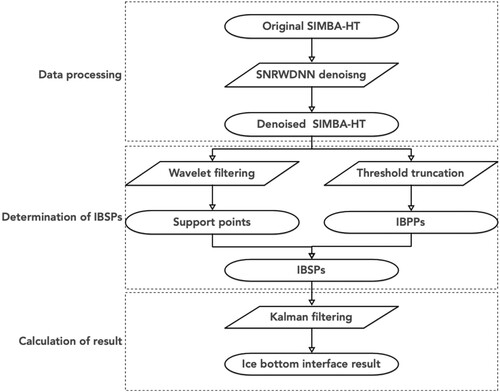
In summary, the NWK approach comprises three parts: denoising data processing, determination of the IBSPs series $P_{sig}$, and the Kalman filter calculation. First, we used the SNRWDNN to remove the stripe noise from the raw extended SIMBA_HT data. Wavelet filtering was then employed to generate the support point set $P_{sup}$, which aided to obtain the dynamic sensor area $\mathrm{\Omega }$ containing information about the ice-bottom interface. Using $\mathrm{\Omega }$, we derived a series of IBSPs, $P_{sig}$, to observe the ice-bottom interface. Finally, by applying the Kalman filter calculation to $P_{sig}$, we obtain the posterior estimate $\tilde{P}$, which represents the actual ice-bottom interface result.

Figure 5. Identified ice-bottom (yellow dashed line) evolution by the neural network, wavelet analysis, and Kalman filtering (NWK) approach. The background represents the original SIMBA_HT time series of all sensors. The sensor numbers are converted into depth using the initial ice surface as a zero-reference level.

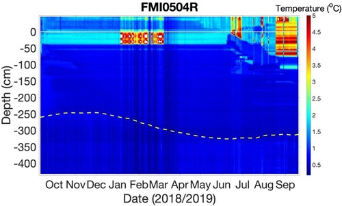
Figure 6. The neural network, wavelet analysis, and Kalman filtering (NWK) approach workflow diagram.

It is important to note that the NWK approach, depicted in Figure 6, is a complex process distinct from the SIMBA_HT algorithm (Liao et al. 2019). While the NWK approach works well in identifying the ice-water interface, it is currently not adequate for identifying the snow surface and snow-ice interface. This is due to the complexity of the natural conditions and environmental disturbances surrounding the sensors, which hinder the clear visibility of the snow surface and snow-ice interface within the SIMBA_HT temperature regimes.

Accurately detecting the positions of the ice surface and bottom is crucial for calculating IT, which is a key input for ice modeling and climate research. The ice-bottom boundary was clearer than the ice surface in the SIMBA_HT data, primarily due to the presence of more noise at the ice surface boundary caused by snow formation. The growth of ice from the bottom is influenced by the energy balance at the ice-water interface, where ice grows when the upward conductive heat flux in the ice is greater than the sensible heat flux from the water to the ice-bottom. Precise digitized information on ice-bottom growth or the delay rate can enhance our understanding of the water-to-ice heat flux (Lei et al. 2010; Yang et al. 2015). The NWK approach provides a general framework for processing the spatiotemporal distribution of Earth’s geophysical datasets and shows potential for tackling generalized edge detection problems.

4. Result and discussion

We applied the NWK approach to 11 time series of SIMBA_HT data (Table 1) and compared the results with those of manual analyzes. To preserve all the edge information, the temperature backgrounds were extracted from the original extended SIMBA_HT data. This ensured that all figures retained all the edge information and displayed the effects of the NWK approach intuitively. In addition to comparing the NWK results of the total working time with those of the manual methods, we conducted a comparative analysis considering different stages of ice evolution. Based on the seasonal and annual cycles, we categorized the IT time series into rapid ice growth, thermal equilibrium (stable), and melting stages. Due to SIMBA operation variations, not all SIMBA_HT data cover every stage. Therefore, we only list the stages covered by SIMBA_HT for each case.

4.1. Sea ice-bottom identification in the Arctic Ocean

FMI0403, FMI0505, FMI0504R, PRIC0903, FMI0509, FMI17R, and FMI0507 were deployed in the Arctic Ocean. Arctic sea ice is frozen seawater that forms in the Arctic Ocean. Sea ice grows dramatically during the winter and melts equally dramatically during the summer. Ice thickness can indicate how vulnerable the ice is to melting and how it functions as a habitat in these ecosystems. However, we lack direct measurements for the extent of sea ice. We compared the ice-bottom results obtained using the NWK approach with manual results (Table 2).

Table 2. Comparison between manual ice thickness results and NWK approach with SIMBA_HT in the Arctic Ocean.

	Stage	Mean Value (cm)		Standard Deviation (cm)		Bias (cm) (NWK)	RMSE (cm)	CORR
		Manual	NWK	Manual	NWK
FMI0403	Total	125.33	128.90	28.23	28.60	3.56	14.41	0.99
	Growth	135.55	139.52	25.22	25.00	3.96	14.41	0.99
FMI0505	Total	209.17	210.61	40.30	39.73	1.44	5.82	0.99
	Growth	182.40	184.76	20.91	21.56	2.36	6.53	0.99
	Stable	247.00	247.03	11.83	9.77	0.04	5.57	0.99
	Decay	252.66	255.04	0.94	1.14	2.37	5.71	0.98
FMI0504R	Total	208.00	206.17	31.19	30.52	−1.83	7.28	0.99
	Growth	191.86	191.19	19.63	19.38	−0.66	3.34	0.99
	Stable	244.00	242.07	5.06	4.82	−1.92	4.18	0.99
	Decay	243.00	239.06	3.21	4.01	−3.93	18.72	0.89
PRIC0903	Total	171.57	174.02	20.28	21.45	2.46	13.54	0.99
	Growth	178.00	181.71	18.30	17.73	3.71	14.90	0.99
FMI0509	Total	131.58	135.59	34.52	33.27	4.01	19.39	0.99
	Growth	146.00	149.37	27.46	26.64	3.37	13.47	0.99
FMI17R	Total	129.50	123.86	8.59	13.38	−5.64	66.85	0.95
	Growth	131.92	127.02	8.94	14.35	−4.90	62.75	0.96
FMI0507	Total	156.27	155.42	8.89	8.38	−0.85	6.39	0.96
	Growth	161.00	159.59	8.66	8.84	−1.40	2.75	0.99

We compared the results of the manual and NWK data for the total working hours as well as for different stages of the devices. The data were divided into three stages: the IT growth season, IT stable stage, and the decay period. Table 2 presents the mean values and standard deviations of the manual and NWK results for the Arctic Ocean. Furthermore, Table 2 also presents the bias, root mean square error (RMSE), and correlation between the manual and NWK results for the Arctic. The average IT was similar to the IT on the starting date. The mean thickness of ice in the Arctic ranged between 1.30-2.09 m, with the thickest and thinnest ice recorded by buoys FMI0505 and FMI17R, respectively. The standard deviation of the manual IT varied between 8.59-40.30 cm. The bias of mean value between the manual and NWK results ranged between −5.64–4.01 cm. The correlations between the manual and NWK IT were 0.95–0.99. The correlation value demonstrated that the ice growth development from the bottom, estimated from the manual results, showed the least difference from the NWF results. Although bottom development was highly consistent, the RMSE ranged between 5.82–66.85 cm, with the highest difference found at buoy FMI17R. NWK also matched well with the manual results during the IT growth seasons, IT stable stages, and decay periods, with the bias of the mean value between the manual and NWK results ranging from −4.09–3.96 cm. The correlations between the manual and NWK IT were 0.89–0.99, where the minimum correlation was found at buoy FMI0504R during the ice decay period. The RMSE ranged from 2.75–62.75 cm.

FMI0403, FMI0507, PRIC0903, FMI0509, and FMI17R mainly worked during the sea ice growth period. The curve of the ice-bottom interface calculated using the NWK approach agrees with the ice/water interface of the SIMBA_HT background fields (Figure 7a, b, c, d, and e). The working cycles of these buoys varied from 126 d (FMI0507) to 378 d (FMI0504R). The initial IT ranged from 126 cm (FMI0403) to 181 cm (FMI0507). A maximum IT of 211 cm (PRIC0903) appeared on April 21, 2019.

Figure 7. (a) FMI0403 SIMBA_HT data and ice-bottom interface. (b) FMI0507 SIMBA_HT data and ice-bottom interface. (c) PRIC0903 SIMBA_HT data and ice-bottom surface. (d) FMI0509 SIMBA_HT data and ice interface surface. (e) FMI17R SIMBA_HT data and ice-bottom interface. (f) FMI0505 SIMBA_HT data and ice-bottom interface. (g) FMI0504R SIMBA_HT data and ice-bottom interface. The yellow dotted curve represents the ice-bottom interface.

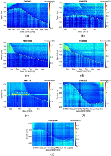
The ice-bottom curve trend of FMI17R was consistent with that of SIMBA_HT. However, from early to mid-October 2018, the results of the NWK approach for the ice-bottom showed that it was thinner than sea ice by approximately 5.6 cm (Figure 7e). The abnormal values recorded by SIMBA_HT were the main cause of this phenomenon.

FMI0505 and FMI0504R were deployed from periods of sea-ice growth to the melting season. The NWK approach agrees well with the SIMBA_HT background temperature during the seasons of sea ice growth (Figure 7f and g). The working cycles of these buoys varied from 367 d (FMI0505) to 378 d (FMI0504R). The initial IT ranged from 211 cm (FMI0505) to 262 cm (FMI0504R). The maximum IT of 327 cm (FMI0504R) appeared on June 7, 2019. However, from mid-August 2019 to mid-September 2019, for FMI0505 and FMI0504R, there was a significant difference between the NWK results and the ice-bottom position determined by the SIMBA_HT background. This is because the detection range $\mathrm{\Omega }$ of the NWK approach is too large during this period. Consequently, numerous fake IBSPs influence the NWK approach results.

Although FMI0403, FMI0507, PRIC0903, FMI0509, and FMI17R were deployed in the Arctic Ocean, their locations differed considerably. Except for PRIC0903, the maximum ITs of FMI0403, FMI0509, FMI17R, and FMI0507 were less than 2 m, and the data acquisition time was mainly concentrated during the sea ice growth seasons and early thermal equilibrium periods. The trend in IT growth and details of the ice-bottom position shown in Figure 7a-e agree with the results of the NWK approach. The results in Figure 8a-e show that the NWK approach can effectively detect the location of the ice-bottom during the growth and thermal equilibrium periods, regardless of whether the IT is greater than 2 m.

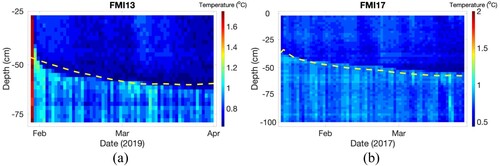
Figure 8. (a) FMI13 SIMBA_HT data and ice-bottom interface. (b) FMI17 SIMBA_HT data and ice-bottom interface. The yellow dotted curve is the ice-bottom interface.

In FMI0505 and FMI0504R, the maximum IT was greater than 2 m, and their data acquisition time were longer than those of others developed in the Arctic Ocean, which covered the growth and thermal equilibrium periods and melting seasons. In the growth and thermal equilibrium periods of sea ice, the ice growth trend and details of the ice-bottom position obtained from NWK matched well with the temperature background field of SIMBA_HT. However, there was a significant deviation between the results of the manual and NWK approaches during the sea ice melting period. This is because, during the melting season, the seawater temperature near the actual ice-bottom was also that of the ice-bottom temperature. Abnormal water temperature affects the judgment and calculation of IBSPs. Moreover, this situation leads to a deviation in the results of the NWK approach during the sea ice melting season.

SIMBA deployed in the Arctic Ocean can observe the entire growth process of sea ice. The ice-bottom grew from November to December and decayed from April to June. During winter, solar radiation decreases and disappears, and oceanic heat is obtained from the inner ocean. The upward conductive heat flux in the ice exceeded the heat flux from the ocean to the ice-bottom, resulting in growth at the ice-bottom. In summer, the increased solar radiation absorbed by the upper ocean contributes to the thawing of the ice-bottom.

4.2. Baltic Sea ice-bottom identification

Two buoys (FMI13 and FMI17) were selected in the Baltic Sea. As the youngest sea globally, the Baltic Sea is shallow, has low salinity, and is surrounded by continents on almost every side. Seasonal sea ice with low bulk salinity and porosity in the Baltic Sea is unique to Arctic sea ice. Apart from sea ice formed from frozen seawater, 35% of sea ice comes from snow. Occasionally, snow and superimposed ice comprise up to 50% of the total IT (Granskog et al. 2006). FMI13 and FMI17 developed in the winters of 2019/2020 and 2017, respectively, during which the ice were very thin. Their number of working cycles is relatively small. FMI13 recorded SIMBA_HT for 65 days, and FMI17 recorded data for 70 days. Representing a low-salinity environment, SIMBA_HT of FMI13 and FMI17 mainly focused on the growth and early thermal equilibrium periods of ice in the Baltic. The initial IT of FMI13 was 43 cm and that of FMI17 was 42 cm. The maximum thickness of sea ice was less than 1 m. The results of the manual and NWK methods are listed in Table 3.

Table 3. Comparison between manual ice thickness results and the NWK approach with SIMBA_HT in the Baltic Sea.

	Stage	Mean Value (cm)		Standard Deviation (cm)		Bias (cm) (NWK)	RMSE (cm)	CORR
		Manual	NWK	Manual	NWK
FMI13	Total	56.64	55.32	4.75	4.38	−1.31	6.74	0.88
	Growth	58.09	56.38	2.59	3.51	−1.70	6.24	0.86
FMI17	Total	51.84	54.25	5.05	6.44	2.41	8.80	0.98
	Growth	53.09	56.00	3.94	4.48	2.91	9.27	0.98

Comparing Tables 2 and 3, it is evident that the mean thickness of Baltic Sea ice is considerably smaller than that of Arctic Ocean ice. Additionally, Table 3 shows a smaller standard deviation compared to Table 2. This observation may be attributed to the fact that the working hours of the Baltic buoys FMI13 and FMI17 were fewer than those of the Arctic Ocean buoys. Furthermore, the correlations between the manual and NWK results for ice-bottom growth in the Baltic Sea are higher than those in the Arctic Ocean. During the IT growth season, the bias of mean value between the manual and NWK results ranged from −1.70–2.91 cm. The correlations between the manual and NWK IT were 0.86−0.98 with the RMSE ranging from 6.24−9.27 cm.

The results of the NWK approach matched well with the ice growth trend of the actual sea ice, but there were differences in the specific values of IT (Figure 8a, b). During the sea ice growth period, the actual sea IT of FMI13 was greater than the IT detected by the NWK approach (4–5 cm). However, for FMI17, the actual IT was lower than that detected using the NWK approach (1–2 cm). Meanwhile, in the early stage of the ice thermal equilibrium period, the IT detected by the NWK approach for FMI13 was thinner than the actual sea IT of 2–3 cm, whereas for FMI17, the IT detected by the NWK approach was thicker than the actual sea IT of 2–4 cm.

These abnormal values were predominantly caused by the abnormal temperature measured initially and the abnormal water temperature near the ice-bottom. In the case of FMI13, the SNRWDNN was used to remove the stripe noise from SIMBA_HT, but it failed to remove the initially abnormal data values. During ice thermal equilibrium, the water temperature below the ice-bottom affects the number of IBPSs, which, in turn, affects the Kalman filter results.

4.3. Lake Orajärvi ice-bottom identification

The buoy data for winter 2014/2015 (FMI09) and winter 2016/2017 (FMI0402) in Lake Orajärvi are analyzed in this subsection. The lake is located in the north of Finland. Snow is present on the lake ice cover every winter, and granular IT ranges from 15% to 80% of the total IT. Buoys FMI09 and FMI0402 also worked for a shorter time in a relatively thin ice environment. In these cases, the NWK approach can also extract the ice-bottom well from SIMBA_HT in boreal lake ice.

The results obtained from buoys FMI09 and FMI0402 are presented in Table 4. The ice-bottom growth rate in the lake was slower than that in the sea, which could be attributed to the heat flux at the water-ice interface. Additionally, the thick snow cover on lake ice every winter results in a snow isolation effect that hinders ice-bottom growth. For FMI09, the mean IT obtained manually was 35.3 cm, whereas the NWK approach yielded a mean thickness of 34.5 cm. The mean IT of FMI0402 was 44.8 and 47.4 cm for the manual and NKW approaches, respectively. The standard deviations of the NKW approach are smaller than those obtained manually. The biases between manual and NWK approaches were −0.75 for FMI09 and 2.62 for FMI0402. The RMSE values differed between the two winters: 32.3 cm in winter 2016/2017 and 2.01 for winter 2014/2015. The correlations between the manual and NKW results for the lake were smaller than those for the sea. During the stable stage of IT, the bias of mean value between the manual and NWK results ranged from −0.48 to −0.54 cm. The correlations between the manual and NWK results ranged from 0.76–0.89, which were lower than the values obtained from the Arctic Ocean and the Baltic Sea. The RMSE values during this period ranged from 6.24–9.27 cm.

Table 4. Comparison between manual ice thickness results and NWK approach with SIMBA_HT in Lake Orajärvi.

	Stage	Mean Value (cm)		Standard Deviation (cm)		Bias (cm) (NWK)	RMSE (cm)	CORR
		Manual	NWK	Manual	NWK
FMI09	Total	35.29	34.54	1.81	1.32	−0.75	2.00	0.75
	Stable	35.45	34.90	1.99	1.27	−0.54	2.02	0.76
FMI0402	Total	44.76	47.38	6.69	2.14	2.62	32.30	0.83
	Stable	49.30	48.82	3.44	2.23	−0.48	3.26	0.89

As shown in Figure 9a and b, there were 53 days of SIMBA_HT data for FMI09, and 101 days of SIMBA_HT data for FMI0402. The initial IT was 30 cm (FMI09) and 31 cm (FMI0402). The maximum IT was 59 cm (FMI0402) on 27/02/2017.

Figure 9. (a) FMI09 SIMBA_HT data and ice-bottom interface. (b) FMI0402 SIMBA_HT data and ice-bottom interface. The yellow dotted curves are the ice-bottom surface.

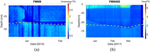
In the boreal lake region, the results obtained by the NWK approach agreed with SIMBA_HT for the growing trend of sea ice (FMI09 and FMI0402). For FMI09, the IT values obtained using the NWK approach are consistent with those of the manual and visual observations in SIMBA_HT (Figure 9a). However, compared with the observation of SIMBA_HT of FMI0402 (Figure 9b), there was a significant deviation between the NWK results and the ice-bottom interface from mid-December to mid-January. We believe that this phenomenon was caused by the working mode of the SIMBA buoy. The sensor chain of SIMBA runs through the ice from top to bottom in a hole. The ice-bottom recondensed with water in the hole during the initial stage. In several cases, we can observe the newly formed ice-bottom (Miller, Cresswell, and Laxon 2003). In contrast, the initial point used by the NWK approach is the initial ice-bottom position when the SIMBA buoy is deployed. It is impossible to reduce the ice-bottom thickness by more than 12 cm daily. However, when the initial starting point is determined, the results of the Kalman filter are continuous. This leads to a significant deviation between the NWK results and the ice-bottom observed in the SIMBA_HT data for FMI0402.

Our NWK approach can be applied to several SIMBA buoy deployment environments including boreal lakes, the Baltic Sea, and the Arctic Ocean. The ice-bottom interface results obtained using the NWK approach exhibited the same pattern as the artificial results in the original SIMBA_HT data. Compared with the RTA algorithm, the NWK approach works well not only in ice-growth seasons but also in melting seasons. The NWK approach can achieve ice-bottom interfaces that match well with the SIMBA_HT heating temperature background fields in both seasons. On the other hand, SIMBA_HT and SIMBA_ET measurements can be affected by the vertical migration of brine within the sea ice layer. Considering this phenomenon, we utilized SIMBA_HT data obtained from the Arctic Ocean, the Baltic Sea, and Lake Orajärvi to investigate the influence of different salinity levels on the performance of our NWK approach. The experimental results showed that the NWK approach has good robustness to vertical migration of brine within the sea ice layer and different salinity levels. This improves the data utilization ratio during the melting season. The deviation in IT between the results obtained by the NWK approach and those observed from SIMBA_HT mainly originates from the water temperature close to the ice-bottom. A water temperature close to the ice-bottom can cause the misjudgment of IBPSs and IBSPs. IBSPs directly affected the NWK results. The abnormal data values of SIMBA_HT and the work mode of SIMBA also influenced the NWK results.

5. Conclusions

In this study, we developed a new approach, NWK, to accurately determine the ice-bottom position from discernible or nebulous ice-water interfaces visible in SIMBA_HT datasets. The identified ice bottom was stable and systematic. The NWK can effectively retrieve the ice/water interface from raw SIMBA_HT data, and the experimental results demonstrate that the NWK approach had good robustness to vertical migration of brine within the sea ice layer and different salinity levels. This was a continuous study after Liao et al. (2019) in which SIMBA_HT data were not used. It has added value to SIMBA applications, improving the understanding of Arctic Sea ice and ice-bottom evolution for seasonal ice-covered seas and boreal lakes. We identified 11 cases of ice-bottom evolution. The detection results agreed with the independent manual analyzes.

SIMAB_HT conveys information regarding material near the ice-bottom. The materials with different heat capacities exhibited different temperature increments after absorbing the same amount of energy. This feature serves as the main principle for detecting ice–water interfaces. Owing to the characteristics of SIMBA_HT, we applied the existing SNRWDNN method to remove the stripe noise from the SIMBA_HT time series. IBPPs and IBSPs are the key links between the denoised SIMBA_HT and the results of this study. Thus, they were proposed to reduce fake interface information and identify potential ice-bottom positions. Wavelet filtering was necessary and helped us to obtain the IBPPs and IBSPs. Finally, the Kalman filter method was used to detect the ice-bottom interfaces from the IBPPs and IBSPs.

The NWK approach performed the best for the Arctic Sea ice conditions, followed by the seasonal ice-covered Baltic Sea and boreal lakes. The Pearson correlation coefficients between the visible and NWK ice-bottom evolutions for the Arctic, Baltic Sea, and Lake Oräjarvi were 0.95, 0.88, and 0.88, respectively. The main error source was the local abnormal SIMBA_HT values, which led to inappropriate IBPPs confirmation and subsequently affected the determination of the actual ice-bottom position. For instance, local data outliers resulted in the incorrect identification of the IBPPs and IBSPs, leading to inaccuracies in the local ice-bottom determination using the NWK approach. However, these errors did not significantly impact NWK ice-bottom detection, especially during the ice-melting seasons. Challenges remain in making the NWK approach reliable when applied to warm and freshwater environments. More reliable IBPPs may be obtained in the Baltic Sea and boreal lakes by using other singularity determination methods to enhance the stability of the NWK approach in thin ice and low-salinity environments.

The data applied in this study revealed a local spatiotemporal continuity resulting from the conservation of physical thermodynamics. Although the NWK approach here is designed for one-dimensional SIMBA_HT data, we believe that the same methodology can be applied to multidimensional data edge detection, such as sea ice lateral evolution due to dynamic and thermodynamic heat and momentum exchange between the ice floe and open water.

Sea ice models require accurate thickness data to accurately represent the physical properties and behaviors of sea ice, including its growth, decay, and movement. This is important for predicting future changes in Arctic ice cover and their associated impacts on global sea level rise, ocean circulation patterns, and climate. SIT data, which are used to monitor changes in sea ice cover over large areas, are important for improving the accuracy of remote sensing measurements. Reliable SIMBA data digital processing and accurate evolution of the ice-bottom may have potentially improved the accuracy of sea ice models and added value by integration with EO datasets to better understand the spatial heterogeneity of Arctic Sea ice (Koo et al. 2021; von Albedyll et al. 2022). Once the ice/water moving boundary is identified, the biogeophysical processes at the ice-bottom can be investigated with the help of numerical modeling, which we aim to do in the next step.

The use of SIMBA buoys deployed in a network that follows the ice drift is an important contribution to observing the seasonal cycle of sea ice. Collecting data on the spatial and temporal variability of sea ice thickness and snow cover is essential for both sea ice modeling and the validation of satellite-derived data sets. The deployment and operation of a network of SIMBA buoys require collaborative efforts between many institutions, especially those organizing field expeditions with icebreakers. Such collaboration was demonstrated during the recent international experiments organized under the INTAROS and CAATEX projects, the CHINARE and NABOS expeditions as well as the MOSAIC drift experiment. In these experiments more than 40 SIMBA buys were operated between 2018 and 2020 (e.g. Lei et al. 2021; Sandven et al. 2022). In the coming years it is necessary to continue and enhance the in situ observations of the annual cycle of sea ice because of its central role in the climate system.

This study focuses on ice bottom identification based on SIMBA heating temperature. It is still challenging to identify the snow-ice interface based on SIMBA heating temperature due to the limited observational methods, which result in unclear and unstable indications in the SIMBA_HT data. Exploring the development of appropriate mathematical identification algorithms for this purpose is another topic that deserves further study.

Acknowledgments

The authors are grateful for the SIMBA data collected from the Chinese National Arctic Research Expedition (CHINARE) 2018, the Nansen and Amundsen Basins Observational System (NABOS) 2018, the RCN-Coordinated Arctic Acoustic Thermometry Experiment (CAATEX) 2018, the international MOSAiC project with the tag MOSAiC20192020 (AF-MOSAiC-1_00, AWI_PS122_1, and AWI_PS122_3), and FMI SIMBA program operations in the Baltic Sea and Lake Oräjarvi.

Data availability statement

The data that support the findings of this study are available from the corresponding author upon reasonable request.

Disclosure statement

No potential conflict of interest was reported by the author(s).

Additional information

Funding

ZL and YJ were supported by the Key-Area Research and Development Program of Guangdong Province, China (No.2021B0101190003) and the Natural Science Foundation of Guangdong Province, China (No. 2022A1515010831). BC was partly supported by the European Union’s Horizon 2020 research and innovation program (727890-INTAROS) in the early phase of SIMBA data analyzes and partly by Polar Regions in the Earth System project (PolarRES, grant 101003590) during the finalization stage of this work.

References

- Canny, J. F. 1983. Finding Edges and Lines in Images. Cambridge: Massachusetts Institute of Technology.
- Chaudhuri, B. B., and B. Chanda. 1984. “The Equivalence of Best Plane Fit Gradient with Robert’s, Prewitt’s and Sobel’s Gradient for Edge Detection and a 4-Neighbour Gradient with Useful Properties.” Signal Processing 6 (2): 143–151. https://doi.org/10.1016/0165-1684(84)90015-X.
- Cheng, Y., B. Cheng, F. Zheng, T. Vihma, A. Kontu, Q. Yang, and Z. Liao. 2020. “Air/Snow, Snow/Ice and Ice/Water Interfaces Detection from High-Resolution Vertical Temperature Profiles Measured by Ice Mass-Balance Buoys on an Arctic Lake.” Annals of Glaciology 61 (83): 309–319. https://doi.org/10.1017/aog.2020.51.
- Cheng, B., T. Vihma, L. Rontu, A. Kontu, H. K. Pour, C. Duguay, and J. Pulliainen. 2022. “Evolution of Snow and ice Temperature, Thickness and Energy Balance in Lake Orajärvi, Northern Finland.” Tellus A: Dynamic Meteorology and Oceanography 66: 21564. https://doi.org/10.3402/tellusa.v66.21564.
- Feldl, N., and T. M. Merlis. 2021. “Polar Amplification in Idealized Climates: The Role of Ice, Moisture, and Seasons.” Geophysical Research Letters 48 (17): e2021GL094130. https://doi.org/10.1029/2021GL094130.
- Filazzola, A., K. Blagrave, M. A. Imrit, and S. Sharma. 2020. “Climate Change Drives Increases in Extreme Events for Lake Ice in the Northern Hemisphere.” Geophysical Research Letters 47 (18): e2020GL089608. https://doi.org/10.1029/2020GL089608.
- Granskog, M., H. Kaartokallio, H. Kuosa, D. N. Thomas, and J. Vainio. 2006. “Sea Ice in the Baltic Sea – A Review.” Estuarine, Coastal and Shelf Science 70 (1-2): 145–160. https://doi.org/10.1016/j.ecss.2006.06.001.
- Guan, J., R. Lai, and A. Xiong. 2019. “Wavelet Deep Neural Network for Stripe Noise Removal.” IEEE Access 7: 44544–44554. https://doi.org/10.1109/ACCESS.2019.2908720.
- Holland, M. M., and L. Landrum. 2021. “The Emergence and Transient Nature of Arctic Amplification in Coupled Climate Models.” Frontiers in Earth Science 9: 719024. https://doi.org/10.3389/feart.2021.719024.
- Jackson, K., J. Wilkinson, T. Maksym, D. Meldrum, J. Beckers, C. Haas, and D. Mackenzie. 2013. “A Novel and Low-Cost Sea Ice Mass Balance Buoy.” Journal of Atmospheric and Oceanic Technology 30 (11): 2676–2688. https://doi.org/10.1175/JTECH-D-13-00058.1.
- Johannessen, O. M., L. Bengtsson, M. W. Miles, S. I. Kuzmina, V. A. Semenov, G. V. Alekseev, A. P. Nagurnyi, et al. 2022. “Arctic Climate Change: Observed and Modelled Temperature and Sea-Ice Variability.” Tellus A: Dynamic Meteorology and Oceanography 56 (4): 328–341. https://doi.org/10.3402/tellusa.v56i4.14418.
- Julier, S. J., and J. K. Uhlmann. 1997. “A New Extension of the Kalman Filter to Nonlinear Systems”. Signal Processing, Sensor Fusion, and Target Recognition. Conference No. 6, Vol. 3068: 182-193.
- Koo, Y., R. Lei, Y. Cheng, B. Cheng, H. Xie, M. Hoppmann, N. T. Kurtz, S. F. Ackley, and A. M. Mestas-Nuñezaet. 2021. “Estimation of Thermodynamic and Dynamic Contributions to Sea Ice Growth in The Central Arctic Using ICESat-2 and MOSAiC SIMBA Buoy Data.” Remote Sensing of Environment 267: 112730. https://doi.org/10.1016/j.rse.2021.112730.
- Kwok, R. 2018. “Arctic Sea Ice Thickness, Volume, and Multiyear Ice Coverage: Losses and Coupled Variability (1958–2018).” Environmental Research Letters 13 (10): 105005. https://doi.org/10.1088/1748-9326/aae3ec.
- Kwok, R., and D. A. Rothrock. 2009. “Decline in Arctic Sea Ice Thickness from Submarine and ICESat Records: 1958–2008.” Geophysical Research Letters 36 (15): L15501. https://doi.org/10.1029/2009GL039035.
- Lang, A., S. Yang, and E. Kaas. 2017. “Sea Ice Thickness and Recent Arctic Warming.” Geophysical Research Letters 44 (1): 409–418. https://doi.org/10.1002/2016GL071274.
- Lei, R., B. Cheng, M. Hoppmann, F. Zhang, G. Zuo, J. K. Hutchings, L. Lin, et al. 2022. “Seasonality and Timing of Sea Ice Mass Balance and Heat Fluxes in the Arctic Transpolar Drift during 2019-2020.” Elementa: Science of the Anthropocene 10 (1): 000089. https://doi.org/10.1525/elementa.2021.000089.
- Lei, R., M. Hoppmann, B. Cheng, G. Zou, D. Gui, Q. Cai, H. J. Belter, and W. Yang. 2021. “Seasonal Changes in Sea Ice Kinematics and Deformation in the Pacific Sector of the Arctic Ocean in 2018/19.” The Cryosphere 15 (3): 1321–1341. https://doi.org/10.5194/tc-15-1321-2021.
- Lei, R., Z. Li, B. Cheng, Z. Zhang, and P. Heil. 2010. “Annual Cycle of Landfast Sea Ice in Prydz Bay, East Antarctica.” Journal of Geophysical Research 115: C02006. https://doi.org/10.1029/2008JC005223.
- Lei, R., H. Xie, J. Wang, M. Leppäranta, I. Jónsdóttir, and Z. Zhang. 2015. “Changes in Sea Ice Conditions Along the Arctic Northeast Passage from 1979 to 2012.” Cold Regions Science and Technology 119: 132–144. https://doi.org/10.1016/j.coldregions.2015.08.004.
- Leppäranta, M. 1983. “A Growth Model for Black Ice, Snow Ice and Snow Thickness in Subarctic Basins.” Hydrology Research 14 (2): 59–70. https://doi.org/10.2166/nh.1983.0006.
- Liao, Z., B. Cheng, J. Zhao, T. Vihma, K. Jackson, Q. Yang, Y. Yang, et al. 2019. “Snow Depth and Ice Thickness Derived from SIMBA Ice Mass Balance Buoy Data Using an Automated Algorithm.” International Journal of Digital Earth 12 (8): 962–979. https://doi.org/10.1080/17538947.2018.1545877.
- Lopez, L. S., B. A. Hewitt, and S. Sharma. 2019. “Reaching a Breaking Point: How Is Climate Change Influencing the Timing of Ice Breakup in Lakes Across the Northern Hemisphere?” Limnology and Oceanography 64 (6): 2621–2631. https://doi.org/10.1002/lno.11239.
- Majumdar, S. J., C. H. Bishop, B. J. Etherton, and Z. Toth. 2002. “Adaptive Sampling with the Ensemble Transform Kalman Filter. Part II: Field Program Implementation.” Monthly Weather Review 130 (5): 1356–1369. https://doi.org/10.1175/1520-0493(2002)130<1356:ASWTET>2.0.CO;2.
- Miller, P. A., D. J. Cresswell, and S. W. Laxon. 2003. “Constraining Sea Ice Model Parameters Using Remote Sensed Sea Ice Thickness Data.” In Proceedins of EGS-AGU-EUG Joint Assembly, Nice, France, 6-11 Apirl, 12182.
- Provost, C., N. Senéchael, J. Miguet, P. Itkin, A. Rösel, Z. Koenig, N. Villacieros-Robineau, and M. A. Granskog. 2017. “Observations of Flooding and Snow-Ice Formation in a Thinner Arctic Sea-Ice Regime During theN-ICE2015 Campaign: Influence of Basal ice Melt and Storms.” Journal of Geophysical Research: Oceans 122 (9): 7115–7134. https://doi.org/10.1002/2016JC012011.
- Rantanen, M., A. Y. Karpechko, A. Lipponen, K. Nordling, O. Hyvärine, K. Ruosteenoja, T. Vihma, and A. Laaksonen. 2022. “The Arctic Has Warmed Nearly Four Times Faster Than the Globe Since 1979.” Communications Earth & Environment 3: 168. https://doi.org/10.1038/s43247-022-00498-3.
- Richter-Menge, J. A., D. K. Perovich, B. C. Elder, K. Claffey, I. Rigor, and M. Ortmeyer. 2006. “Ice Mass-Balance Buoys: A Tool for Measuring and Attributing Changes in the Thickness of the Arctic Sea-Ice Cover.” Annals of Glaciology 44: 205–210. https://doi.org/10.3189/172756406781811727.
- Sallila, H., S. L. Farrell, J. McCurry, and E. Rinne. 2019. “Assessment of Contemporary Satellite Sea Ice Thickness Products for Arctic Sea Ice.” The Cryosphere 13 (4): 1187–1213. https://doi.org/10.5194/tc-13-1187-2019.
- Sandven, S., H. Sagen, R. Pirazzini, A. Beszczynska-Möller, F. Danielsen, P. Gonçalves, G. Ottersen, et al. 2022. “Deliverable 1.11 Final synthesis report. Zenodo.”.
- Shih, M. Y., and D. C. Tseng. 2005. “A Wavelet-Based Multiresolution Edge Detection and Tracking.” Image and Vision Computing 23 (4): 441–451. https://doi.org/10.1016/j.imavis.2004.11.005.
- Smith, D. M., J. A. Screen, C. Deser, J. Cohen, J. C. Fyfe, J. García-Serrano, T. Jung, et al. 2019. “The Polar Amplification Model Intercomparison Project (PAMIP) Contribution to CMIP6: Investigating the Causes and Consequences of Polar Amplification.” Geoscientific Model Development 12 (3): 1139–1164. https://doi.org/10.5194/gmd-12-1139-2019.
- von Albedyll, L., S. Hendricks, R. Grodofzig, T. Krumpen, S. Arndt, H. J. Belter, B. Cheng, et al. 2022. “Thermodynamic and Dynamic Contributions to Seasonal Arctic Sea Ice Thickness Distributions from Airborne Observations.” Elementa: Science of the Anthropocene 10 (1): 00074. https://doi.org/10.1525/elementa.2021.00074.
- Wagner, P., and K. Frame. 2015. Combining Radarsat, Envisat, AMSR-E, and ASPeCt Ship-Based Ice Observations to Determine Ice Concentration at 90°W Longitude in the Bellingshausen Amundsen Sea for SIMBA 2007. Newark: University of Delaware.
- Wang, Q., Z. Li, R. Lei, P. Lu, and H. Han. 2018. “Estimation of the Uniaxial Compressive Strength of Arctic Sea Ice during Melt Season.” Cold Regions Science and Technology 151: 9–18. https://doi.org/10.1016/j.coldregions.2018.03.002.
- Wever, N., K. Leonard, T. Maksym, S. White, M. Proksch, and J. T. M. Lenaerts. 2021. “Spatially Distributed Simulations of the Effect of Snow on Mass Balance and Flooding of Antarctic Sea Ice.” Journal of Glaciology 67 (266): 1055–1073. https://doi.org/10.1017/jog.2021.54.
- Weyhenmeyer, G. A. 2001. “Warmer Winters: Are Planktonic Algal Populations in Sweden’s Largest Lakes Affected?” AMBIO: A Journal of the Human Environment 30 (8): 565–571. https://doi.org/10.1579/0044-7447-30.8.565.
- Weyhenmeyer, G. A. 2009. “Do Warmer Winters Change Variability Patterns of Physical and Chemical Lake Conditions in Sweden?” Aquatic Ecology 43 (3): 653–659. https://doi.org/10.1007/s10452-009-9284-1.
- Wilkinson, M. D., M. Dumontier, I. J. J. Aalbersberg, G. Appleton, M. Axton, A. Baak, N. Blomberg, et al. 2016. “The FAIR Guiding Principles for Scientific Data Management and Stewardship.” Scientific Data 3: 160018. https://doi.org/10.1038/sdata.2016.18.
- Xiao, L., and S. Boyd. 2004. “Fast Linear Iterations for Distributed Averaging.” Systems & Control Letters 53 (1): 65–78. https://doi.org/10.1016/j.sysconle.2004.02.022.
- Yang, Y., M. Leppäranta, Z. Li, B. Cheng, M. Zhai, and D. Demchev. 2015. “Model Simulations of the Annual Cycle of the Landfast Ice Thickness in the East Siberian Sea.” Advances in Polar Science (In English) 26 (2): 168–178. https://doi.org/10.13679/j.advps.2015.2.00168.
- Zuo, G., Y. Dou, and R. Lei. 2018. “Discrimination Algorithm and Procedure of Snow Depth and Sea Ice Thickness Determination Using Measurements of the Vertical Ice Temperature Profile by the Ice-Tethered Buoys.” Sensors 18 (12): 4162. https://doi.org/10.3390/s18124162.
- Zygmuntowska, M., P. Rampal, N. Ivanova, and L. H. Smedsrud. 2014. “Uncertainties in Arctic Sea Ice Thickness and Volume: New Estimates and Implications for Trends.” The Cryosphere 8 (2): 705–720. https://doi.org/10.5194/tc-8-705-2014.