A multi-scale path-planning method for large-scale scenes based on a framed scale-elastic grid map

ABSTRACT

Environment modeling serves as the foundation for path planning in unmanned systems. Single-scale maps have many nodes and impose large memory requirements; tree-based multi-scale grid maps used for representing large-scale urban scenes have limited aggregation ability in the presence of dimensional anisotropy. This study proposes a novel multi-scale map-construction method based on a scale-elastic discrete grid structure. The method provides more flexible node aggregation in grid-based representations, reducing the number of grid and border-grid nodes while maintaining the same modeling accuracy. Furthermore, a novel multi-scale A* path-planning algorithm that modifies the neighborhood-expansion phase of A* is proposed to reduce the number of algorithm search nodes in framed multi-scale maps while ensuring optimal path planning. The experimental results demonstrate that the proposed map-construction method requires 71.5% fewer grids and 10.8% fewer border grids than framed-octree grid maps in three-dimensional scenarios with the same modeling accuracy. Consequently, memory requirements are smaller, making this method more efficient on devices with limited performance. The multi-scale A* algorithm also improves path-planning efficiency by reducing the number of search nodes. The proposed method is suitable for path planning in large-scale and complex urban scenes.

KEYWORDS:

• Grid map
• path planning
• scale-elastic grid structure
• voxel-based modeling

1. Introduction

Recently, unmanned aerial vehicles (UAVs) have been widely used in various fields, including agricultural irrigation (Tsouros, Stamatia, and Sarigiannidis 2019), anti-terrorism operations (Wang et al. 2021), power inspection (Jordan et al. 2018), and 3D reconstruction (Liu et al. 2022). In all these applications, path planning is fundamental if the UAVs are to execute their tasks successfully. Despite significant advances, path planning in large-scale operational environments continues to present a substantial challenge (Xie et al. 2021). For applications such as coverage-path planning (Chen et al. 2021) or route optimization (Xu et al. 2023) in urban settings characterized by intricate terrain, numerous buildings, and large areas, the generation of efficient and precise paths remains a problem of the utmost importance (Zhang et al. 2022).

This research introduces a novel approach to creating multi-scale maps. A scale-elastic discrete grid structure is employed, enhancing the flexibility of node aggregation in grid-based representations. This innovation addresses the limitations of grid aggregation in existing tree-based multi-scale path-planning structures, offering a more efficient way to aggregate nodes at different scales. Furthermore, a specialized multi-scale A* algorithm has been developed, tailored to the characteristics of these multi-scale maps. The algorithm optimizes the neighborhood-expansion phase of traditional A* search, significantly reducing the number of search nodes required. By integrating these two methods, the research provides a comprehensive solution to the problems of multi-scale map construction and path planning, offering improved performance and scalability for applications in complex and large-scale environments.

The remainder of this paper is organized as follows: Section II provides an overview of relevant research in environmental modeling and multi-scale path planning, highlighting existing challenges. Section III describes the methodology and theoretical framework of the proposed approach. Section IV presents the experimental setup and results. Finally, Section V summarizes the research findings and suggests potential research directions.

2. Related work

Path planning in large-range scenes has been extensively studied in the fields of robotics and navigation. In this section, we review related work in the context of environment modeling and path finding. These are closely related because certain path-planning algorithms can only be applied to specific scene models (Radmanesh et al. 2018).

Environment modeling entails the transformation of a real-world planning environment into a digital representation that is amenable to computational processing. An accurate and appropriate model provides a complete and relevant description of the environment, leading to reduced computational consumption and improved path-planning efficiency (Zhang, Lin, and Chen 2018). Current environment-modeling methods include approaches based on topology (Ivanov 2018; Yan, Zlatanova, and Diakité 2021) and cell decomposition (Pun-Cheng, Tang, and Cheung 2007; Tsatcha, Saux, and Claramunt 2014), as well as the probabilistic roadmap method (Hauer et al. 2015). Topology-based methods can effectively reduce the complexity of planning environments, transforming a path planning problem into a connectivity problem in a lower-dimensional space, thus achieving fast and efficient path planning. However, these methods are most effective in environments with apparent characteristics and sparse obstacles. They face challenges in maintaining topology information when the obstacle configuration changes in the environment (Zhang, Lin, and Chen 2018). Probabilistic roadmap methods have similar problems. The cell-decomposition approach dissects the planning environment into discrete cells of predetermined shapes (e.g. rectangles) and sizes. It constructs an undirected graph where each cell is a vertex and the adjacency between cells is represented by edges. Subsequently, search-based algorithms (Cormen et al. 2022) are employed to plan paths through this graph. Typically, a uniform square grid is used to create undirected maps with simple adjacency relationships that are easy to design and implement (Han et al. 2022). These maps perform well when dealing with small-scale, low-dimensional scenes (Tanzmeister et al. 2014; Yoon et al. 2015). However, when the planning-environment dimensionality is high, the scene range is large, the grid size is small, or the scene contains extensive unobstructed areas, a uniform grid requires a vast number of discrete grid cells, lowering the search efficiency (Hauer et al. 2015; Namdari, Hejazi, and Palhang 2016). From experimental statistics (Namdari, Hejazi, and Palhang 2016), the average time needed by A* algorithm on uniform grids in 2D environment increases exponentially as the number of grids increases. In a $1024\times 1024$ 2D grid environment, path planning with A* algorithm takes approximately 30 s.

One common strategy for overcoming these limitations is to decompose the environment into different levels of granularity and plan paths at multiple scales. For example, some methods divide the environment into grids of different resolutions, allowing for efficient path planning at both global and local scales. These methods are classified as either top-down or bottom-up (Hauer et al. 2015). Top-down methods typically begin by identifying a path at the coarsest resolution, which is then iteratively refined to achieve greater precision (Hauer et al. 2015; Pai and Reissell 1998; Zhang et al. 2022); bottom-up methods address the problem at each node at the finest resolution level and combine the results at different resolution levels (Chen, Szczerba, and Uhran 1997; Namdari, Hejazi, and Palhang 2016). While top-down methods might not always guarantee the most optimal path owing to their initial broad planning approach, bottom-up methods offer a higher degree of precision path planning (Li, Zhao, and Zhou 2014). However, this precision comes at the cost of efficiency, as these methods necessitate a comprehensive search across multiple, finer resolution levels (Nelson, Corah, and Michael 2018).

To reconcile the efficiency and accuracy of path planning, a hybrid approach using a framed-quadtree data structure has been proposed to merge the accuracy of fine-resolution grid-based path planning with the efficiency of spatial quadtree-based methods (Chen, Szczerba, and Uhran 1997). This approach operates on a bottom-up principle and can generate shorter and smoother paths than single-scale grid maps (SGM) (Namdari, Hejazi, and Palhang 2016). Similarly, a framed-octree can be constructed in three-dimensional (3D) space for path planning (Szczerba, Chen, and Uhran 1998). However, because the construction of existing framed multi-scale grid maps (FMGM) are based on tree-based structures, aggregation can be performed only when there are no obstacles within the map range corresponding to all child nodes of a node (Chen et al. 2023).

Owing to limitations in aggregation capabilities, the aforementioned methods often face significant challenges in representing real-world environments that exhibit anisotropy (Lei et al. 2022). This anisotropy means that the distribution density of the data in the real environment, especially urban data, is different in the horizontal direction and the elevation direction. This characteristic leads to an abundance of redundant nodes in the representation of open spaces in existing tree-based multi-scale grid maps, increasing the number of nodes and grids required for environmental modeling and consequently diminishing the efficiency of the path-planning algorithm.

Another strategy is to adjust the neighborhood expansion method of search-based algorithms. Neighborhood expansion is one of the key steps in the search-based algorithm process, that significantly affects the shape of the search path, optimality of the search path, and search efficiency (Hormazábal et al. 2021). For example, in a 4-neighborhood search, the minimum turn angle of the search path is 90°, while in an 8-neighborhood search, the minimum turn angle of the search path is 45°. Owing to the restriction of the minimum turn angle, the path planning lengths based on 4 – and 8-neighborhood are $\sqrt{2}$ and $\sqrt{4-4\sqrt{2}}$ times of the optimal planning paths at any angle, respectively (Bailey et al. 2015). The planning case of a $2^k$-neighborhood has also been studied (Rivera et al. 2020). To find higher-quality solutions while still using graph search algorithms, researchers have extended ${\mathrm{A}}^{\ast }$ to include moves with greater angular diversity and have proposed path planning methods that can directly consider arbitrary angles (Daniel et al. 2010; Harabor et al. 2016). However, these studies have primarily focused on graph search algorithms on single-scale grid maps, while there is still little research on improvements based on multi-scale grid maps.

3. Methodology

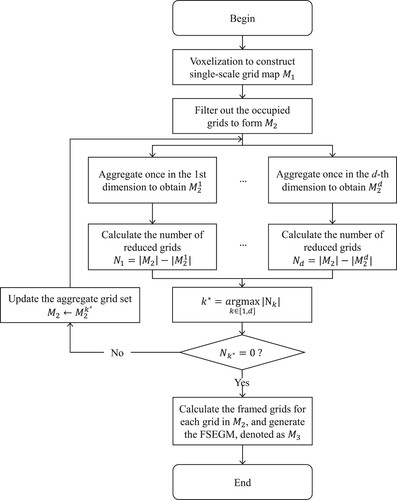
The methodology chapter is divided into two sections. The first section outlines the construction of a Framed scale-elastic grid map, which is employed for environmental modeling. The second section presents a multi-scale A* algorithm based on the constructed map. An overview of the complete multi-scale path-planning scheme is shown in Figure 1. The symbols used in this study are defined in Table 1.

Figure 1. Research schematic describing multi-scale path planning for large-scale scenes.

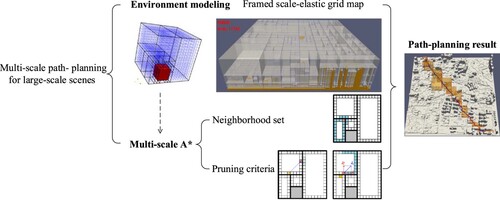
Table 1. Symbols and descriptions.

Symbol	Description
$n$	Finest-resolution grid nodes in framed multi-scale grid map
$n_{\mathrm{cur}}$	Node that currently requires neighborhood expansion
$n_{\mathrm{pre}}$	Predecessor node of $n_{\mathrm{cur}}$node
$n_{\mathrm{next}}$	Post node of $n_{\mathrm{cur}}$ node
${\mathcal{N}}_1\left(n\right)$	The set of neighborhoods formed by the spatially adjacent nodes of $n$
${\mathcal{N}}_2\left(n\right)$	The set of boundary grids of multi-scale nodes corresponding to $n$
$\mathcal{N}\left(n\right)$	The set of neighborhoods of node $n$, $\mathcal{N}\left(n\right)={\mathcal{N}}_1\left(n\right)\cup {\mathcal{N}}_2\left(n\right)$
$s$	Starting node in path-planning problems
$t$	Target node in path-planning problems
$p\left(s,t\right)$	The sequence of paths from $s$ to $t$, $p\left(s,t\right)=\{s=n_0,n_1,n_2,\dots ,n_{m-1},n_m,t=n_{m+1}$}
$d\left(n_i,n_j\right)$	Distance between nodes $n_i$ and $n_j$
$b\left(n\right)$	Multi-scale grid node corresponding to $n$

3.1. Framed scale-elastic grid map

3.1.1. Scale-elastic discrete grid structure

The scale-elastic discrete grid structure (Lei et al. 2022) is an axis-aligned discrete grid system (Gibb et al. 2022; ISO 19170–4 2023) that uses a pairwise orthogonal coordinate frame for spatial division. This structure enables independent divisions in different directions, making it suitable for node formation in high-dimensional grids. The fundamental principle of this structure involves the construction of a binary tree in each dimension to represent the position information of the grid. By combining the information from each dimension, the shape and position of the target grid in high-dimensional space can be uniquely determined. The 2D grid space-division method is illustrated in Figure 2 The spatial partitioning and grid-labeling capabilities of the quadtree spatial partitioning method are demonstrated in Figure 2(e) and (f). The scale-elastic discrete grid structure provides excellent marking capability and can potentially enhance the efficiency and accuracy of high-dimensional data processing.

Figure 2. Illustration of 2D spatial division and identification based on the scale-elastic discrete grid structure. $L_1$ and $L_2$ denote the subdivision levels in the two directions, while $C_1$ and $C_2$ represent coordinates under different subdivision levels. The gray area in the figures depicts the range of grid identification, and corresponding numbers indicate the coordinates of the grid. (a) $L_1=0$, $L_2=1$ (b) $L_1=1$, $L_2=0$ (c) $L_1=0$, $L_2=2$ (d) $L_1=2$, $L_2=0$ (e) $L_1=1$, $L_2=1$ (f) $L_1=2$, $L_2=2$.

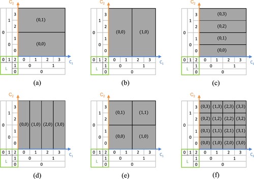
As discussed previously, the scale-elastic discrete grid structure provides flexible marking capabilities, allowing various map-construction methods for the same environment. For instance, Figure 2(a) and (d) shows two distinct map-construction methods that produce different numbers of grids and border grids. Lei et al. (2022) introduced a grid-aggregation algorithm based on a scale-elastic discrete grid structure to address the need for data organization; however, their depth-first aggregation approach overlooks the necessity of path planning. Consequently, this paper investigates a grid aggregation and map construction method based on a scale-elastic discrete grid framework, which results in a sparser node count and is more attuned to the requirements of path planning.

3.1.2. Parent-grid calculation and grid-aggregation method

The subdivision level and coordinates of a grid in the k-th direction are denoted as $L_k$ and $C_k$, respectively. Different directions result in different parental grids. Let $g_f^k$ represent the parent grid of $g$ in the k-th dimension. Therefore, we state that: (1) $\{\begin{array}{c}{p}_L^k\left(g_f^k\right)=p_L^k\left(g\right)-1\\ p_C^k\left(g_f^k\right)=p_C^k\left(g\right)\end{array}$(1) Here, ⌊*⌋ represents the floor operation. 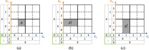$p_L^k(\ast )$ and $p_C^k(\ast )$ represents the subdivision level and coordinates of a grid int the $k$-th direction, respectively. For example, in the two-dimensional case shown in Figure 3, the gray grid $g$ in (a) has grid levels and coordinates $(L_1,L_2,{\mathrm{C}}_1,{\mathrm{C}}_2)=\left(2,2,1,1\right)$. Its parent grid $g_f^1$ in the $C_1$ dimension is the gray grid in (b), with grid levels and coordinates $\left(L_1,L_2,C_1,C_2\right)=\left(1,2,0,1\right)$. The parent grid $g_f^2$ of $g$ in the $C_2$ dimension is the gray grid in (c), with grid levels and coordinates $\left(L_1,L_2,C_1,C_2\right)=\left(2,1,1,0\right)$.

Figure 3. Parent grids in different directions. The gray grids in (b) and (c) are the parent grids of the gray grid in (a) in the $C_1$ and $C_2$ axis directions, respectively. (a) $(L_1,L_2,{\mathrm{C}}_1,{\mathrm{C}}_2)=\left(2,2,1,1\right)$ (b) $(L_1,L_2,{\mathrm{C}}_1,{\mathrm{C}}_2)=\left(1,2,0,1\right)$ (c) $(L_1,L_2,{\mathrm{C}}_1,{\mathrm{C}}_2)=\left(2,1,1,0\right)$.

The aggregation process for a set of grids $G=\left\{g_1,g_2,\dots ,g_m\right\}$ in the k-th-direction is performed as follows:

Table

Algorithm 1: Grids Aggregation in the $k$-th Direction
Input: A set of grids $G=\left\{g_1,g_2,\dots ,g_m\right\}$, the direction for aggregation $k$
Output: A set of aggregated grids $G_f^k$
1: TypeA_Correspondences$=\left[\right]$
2: TypeB_Correspondences$=\left[\right]$
3: AggregatedGrids$=\left[\right]$
4: for each grid $g_i$in G do
5:    // Calculate the parent grid of $g_i$ in the $k$-th direction
6:    $g_{\mathrm{if}}^k=$Calculate parent grid ($g_i$, $k$)
7:    TypeA_Correspondences.append (($g_{\mathrm{if}}^k$, $g_i$))
8: end for
9: // Merge type A correspondences with the same parent grid into type B correspondences
10: for each correspondence ($g_f^k,g$) in TypeA_Correspondences do
11:    Related_Correspondences = Filter TypeA_Correspondences with parent grid $g_f^k$
12:    if the size of Related_Correspondences > 1 then
13:       Child_Grids = Extract child grids from Related_Correspondences
14:       TypeB_Correspondences.append (($g_f^k$, Child_Grids))
15:       for each correspondence in Related_Correspondences do
16:           TypeA_Correspondences.remove (correspondence)
17:       end for
18:    end if
19: end for
20: // Generate aggregated grids
21: for each correspondence ($g_f^k$, $g$) in TypeA_Correspondences do
22:    AggregatedGrids.append ($g$)
23: end for
24: for each correspondence ($g_f^k$, Child_Grids) do
25:    AggregatedGrids.append $g_{\mathrm{if}}^k)$
26: end for
27: return AggregatedGrids

For example, consider the grid set shown in Figure 4(a). It consists of six grid elements. The aggregation process along the $C_1$ axis is illustrated in Figure 4(d). Initially, six sets of type A binary correspondence are obtained after calculating the parent grid. (Here $g_1$ and $g_2$ share the same parent grid, and $g_4$ and $g_5$ share the same parent grid.) After merging the correspondences, $\left(g_{1f}^1,g_1\right)$ and $\left(g_{2f}^1,g_2\right)$ generate a new correspondence $\left(g_{1f}^k,\left(g_1,g_2\right)\right)$, and $\left(g_{4f}^1,g_4\right)$ and $\left(g_{5f}^1,g_5\right)$ generate a new correspondence $\left(g_{4f}^k,\left(g_4,g_5\right)\right)$. Finally, the grid elements are extracted from the different types of correspondences to obtain a set of aggregation results $\left\{g_{1f}^1,g_3,g_{4f}^1,g_6\right\}$.

Figure 4. Illustration of grid-set aggregation.

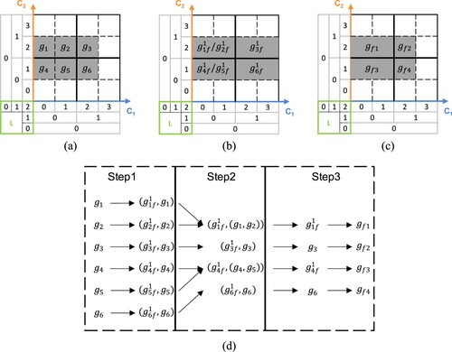
This aggregation process fully harnesses the independent and concurrent characteristics of the grids, which can enhance aggregation efficiency through a parallel framework.

3.1.3. Framed scale-elastic grid map-construction method

To reduce the number of nodes searched by the search-based path-planning algorithm, a FMGM should have as few grids and border grids as possible. This study proposes employing a greedy algorithm comprising following steps; the corresponding flowchart is shown in Figure 5.

Figure 5. Flow chart for construction of framed scale-elastic grid map (FSEGM).

Table

Algorithm 2: Generate Framed Scale-elastic Gird Map
Input: A single-scale grid map $M_1$ at the finest resolution level
Output: Framed scale-elastic grid map $M_3$
1: $M_2=$Filter out the occupied grids from $M_1$
2: repeat
3:    for $k$ = 1 to $d$ do
4:       $M_2^k=$AggregateGrids ($M_2$, $k$)
5:      $N_k=\left|M_2\right|-\left|M_2^k\right|$
6:    end for
7:   $k^{\ast }=\underset{k\in \left[1,d\right]}{\mathrm{argmax}}\left(N_k\right)$
8: until $N_{k^{\ast }}=0$
9: $M_2=M_2^{k^{\ast }}$
10: $M_3=\left[\right]$
11: for each grid $g$ in $M_2$ do
12:    FramedGrids$=$Cal the framed grids of $g$
13:    $M_3$.append (FramedGrids)
14: end for
15: return $M_3$

3.1.4. Example

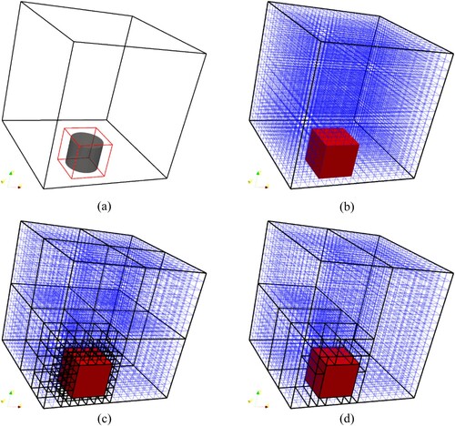
In the 16$\times$16$\times$16 environment shown in Figure 6(a), a gray obstacle is present at the bottom. Assuming that the border grid size is $1\times 1$, a single-scale grid map of this environment is shown in Figure 6(b); it uses 4032 grids to represent the barrier-free area. The corresponding framed-octree map is shown in Figure 6(c); it uses 105 grids and 2488 border grids to represent the barrier-free area. By contrast, the FSEGM shown in Figure 6(d) uses only 17 grids and 2064 border grids to represent the same area.

Figure 6. Various grid maps of the same environment. The blue and red grids represent barrier-free and barrier areas, respectively. (a) example scenario (b) single-scale grid map (c) framed-octree grid map (d) FSEGM.

3.2. Multi-scale A* path-planning algorithm based on an FMGM

Path-planning algorithms and environment-representation methods are often paired together. In the case of grid-based maps, the A* algorithm is widely used and considered the most reliable. This section first examines the inherent challenges associated with the direct application of the A* algorithm to FMGMs. Following this analysis, we leverage the distinctive attributes of FMGMs to introduce a novel multi-scale A* path planning algorithm. This algorithm adapts the neighborhood-expansion phase of the traditional A* algorithm to suit the FMGM framework. (Other intelligent path planning algorithms could be tailored in a similar way to accommodate FMGM, but this falls outside the scope of the present study.)

3.2.1. Neighborhood set

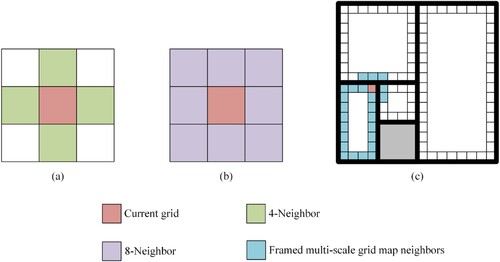
In the A* algorithm, specific criteria are given for the inclusion of other nodes in the neighborhood of the current one. If a neighboring node satisfies these criteria, its heuristic value is calculated and the node is subsequently added to the exploration queue. In a single-scale grid map, the neighborhood typically includes only spatially adjacent nodes, leading to four – or eight-grid neighborhoods in 2D maps and six – or twenty-six-grid neighborhoods in 3D maps.

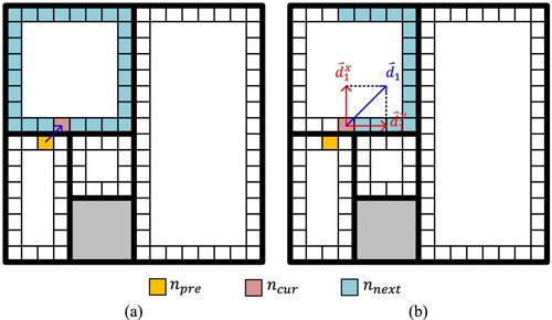
By contrast, FMGMs (i.e. multi-scale maps utilizing frame structures, such as framed-quadtree grid maps, framed-octree grid maps, and the FSEGMs considered in this study) define the neighborhood of the current node more expansively to include not only spatially adjacent nodes but also all border grids within the same multi-scale grid. Figure 7 illustrates neighborhoods in different types of 2D maps. The number of neighbors in an FMGM is substantially larger than in a single-scale map.

Figure 7. Different types of neighborhoods in a 2D environment.

Improperly defined neighborhood-expansion criteria can lead to an excessive number of grids being explored, compromising the efficiency of the path-planning process. To address this, the present study enhances path-planning efficiency through the implementation of pruning principles and the integration of FMGM characteristics. The pruning criteria are based on the scope of the neighborhood set and the directionality of exploration. This curtails the number of grids subjected to exploration within the neighborhood.

3.2.2. Pruning criteria

Neighborhood range pruning. If the multi-scale grid nodes corresponding to the current node $n_{\mathrm{cur}}$ and its predecessor node $n_{\mathrm{pre}}$ are the same, that is, $b\left(n_{\mathrm{cur}}\right)=b\left(n_{\mathrm{pre}}\right)$, then the criterion for ensuring the optimality of the planned path is given in Equation(2) (2) $b\left(n_{\mathrm{next}}\right)\ne b\left(n_{\mathrm{cur}}\right),b\left(n_{\mathrm{cur}}\right)=b\left(n_{\mathrm{pre}}\right)$(2) Let the set of nodes to be explored at this time be $S_1$. Based on the criterion in Equation (2(2) $b\left(n_{\mathrm{next}}\right)\ne b\left(n_{\mathrm{cur}}\right),b\left(n_{\mathrm{cur}}\right)=b\left(n_{\mathrm{pre}}\right)$(2) ) the formula for calculating $S_1$ is shown in Equation (3(3) $=\left\{x|x\in {\mathcal{N}}_1\left(n_{\mathrm{current}}\right)-{\mathcal{N}}_2\left(n_{\mathrm{current}}\right)\right\}$(3) ). $S_1=\left\{x|x\in \mathcal{N}\left(n_{\mathrm{cur}}\right),b\left(x\right)\ne b\left(n_{\mathrm{cur}}\right)\right\}$ $=\left\{x|x\in {\mathcal{N}}_1\left(n_{\mathrm{cur}}\right),b\left(x\right)\ne b\left(n_{\mathrm{cur}}\right)\right\}$ $\cup \left\{x|x\in {\mathcal{N}}_2\left(n_{\mathrm{cur}}\right),b\left(x\right)\ne b\left(n_{\mathrm{cur}}\right)\right\}$ $=\left\{x|x\in {\mathcal{N}}_1\left(n_{\mathrm{current}}\right),b\left(x\right)\ne b\left(n_{\mathrm{cur}}\right)\right\}$ (3) $=\left\{x|x\in {\mathcal{N}}_1\left(n_{\mathrm{current}}\right)-{\mathcal{N}}_2\left(n_{\mathrm{current}}\right)\right\}$(3)

In other words, if $b\left(n_{\mathrm{cur}}\right)=b\left(n_{\mathrm{pre}}\right)$, the expansion of the neighborhood only considers the elements in the difference between ${\mathcal{N}}_1\left(n\right)$ and ${\mathcal{N}}_2\left(n\right)$.

That the criterion in Equation (2(2) $b\left(n_{\mathrm{next}}\right)\ne b\left(n_{\mathrm{cur}}\right),b\left(n_{\mathrm{cur}}\right)=b\left(n_{\mathrm{pre}}\right)$(2) ) ensures optimality of the planned path can be proven by the method of contradiction. Let $p^{\ast }\left(s,t\right)=\left\{s=n_0,n_1^{\ast },n_2^{\ast },\dots ,n_k^{\ast },t=n_{k+1}\right\}$ be the optimal path from $s$ to $t.$ Assume that there exists an $i\in \left[1,k\right]$ such that $b\left(n_{i-1}\right)=b\left(n_i\right)=b\left(n_{i+1}\right)$. Construct a new path $p^{\mathrm{\prime }}\left(s,t\right)=\left\{s=n_0,\dots ,n_{i-1}^{\ast },n_{i+1}^{\ast },\dots ,n_k^{\ast },t=n_{k+1}\right\}$. By the triangle inequality, (4) $d\left(n_{i-1}^{\ast },n_{i+1}^{\ast }\right)<d\left(n_{i-1}^{\ast },n_i^{\ast }\right)+d\left(n_i^{\ast },n_{i+1}^{\ast }\right)$(4) Therefore, the path cost of $p^{\mathrm{\prime }}\left(s,t\right)$ is lower than that of $p^{\ast }\left(s,t\right)$, which contradicts the optimality of the latter. Thus, the assumption is invalid, indicating that the criterion corresponding to Equation (2(2) $b\left(n_{\mathrm{next}}\right)\ne b\left(n_{\mathrm{cur}}\right),b\left(n_{\mathrm{cur}}\right)=b\left(n_{\mathrm{pre}}\right)$(2) ) can ensure the optimality of the planned path.

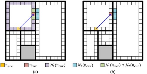
Figure 8(a) illustrates a case without pruning, where 31 elements in $\mathcal{N}\left(n_{\mathrm{cur}}\right)$ must be expanded. Figure 8(b) indicates that with neighborhood pruning, only three elements in $\mathcal{N}\left(n_{\mathrm{cur}}\right)$ must be expanded.

Figure 8. Illustration of neighborhood range pruning in a 2D environment. (a) Range of $\mathcal{N}\left(n_{\mathrm{cur}}\right)$ without pruning, (b) Range of nodes to be explored ($S_1$) after neighborhood range pruning.

Pruning exploration directions. If the multi-scale grid nodes corresponding to $n_{\mathrm{cur}}$ and $n_{\mathrm{pre}}$ are different, that is $b\left(n_{\mathrm{cur}}\right)\ne b\left(n_{\mathrm{pre}}\right)$, let ${d^{\rightharpoonup }}_1,{d^{\rightharpoonup }}_2$ be the direction vectors from $n_{\mathrm{pre}}$ to $n_{\mathrm{cur}}$ and from $n_{\mathrm{cur}}$ to $n_{\mathrm{next}}$, respectively. The projections of these vectors onto the coordinate axes are ${d^{\rightharpoonup }}_1^x,{d^{\rightharpoonup }}_1^y$ and ${d^{\rightharpoonup }}_2^x,{d^{\rightharpoonup }}_2^y$. Then the criteria for ensuring the optimality of the planned path when expanding the neighborhood are (5) $\{\begin{array}{c}{d^{\rightharpoonup }}_1^x\cdot {d^{\rightharpoonup }}_2^x\ge 0\\ {d^{\rightharpoonup }}_1^y\cdot {d^{\rightharpoonup }}_2^y\ge 0\end{array},b\left(n_{\mathrm{next}}\right)=b\left(n_{\mathrm{cur}}\right)$(5) These criteria indicate that considering all the elements in set ${\mathcal{N}}_2\left(n_{\mathrm{cur}}\right)$ is unnecessary; only those elements that are consistent with the movement direction of the current node along each coordinate axis must be considered.

Figure 9(a) illustrates a case without pruning, where 27 elements in ${\mathcal{N}}_2\left(n_{\mathrm{cur}}\right)$ must be expanded. Figure 9(b) shows that with direction pruning only 15 elements in ${\mathcal{N}}_2\left(n_{\mathrm{cur}}\right)$ must be expanded.

Figure 9. Illustration of exploration-direction pruning in a 2D environment. (a) Range of ${\mathcal{N}}_2\left(n_{\mathrm{cur}}\right)$ without pruning, (b) Range of ${\mathcal{N}}_2\left(n_{\mathrm{cur}}\right)$ after directional pruning.

That the criterion in Equation (5(5) $\{\begin{array}{c}{d^{\rightharpoonup }}_1^x\cdot {d^{\rightharpoonup }}_2^x\ge 0\\ {d^{\rightharpoonup }}_1^y\cdot {d^{\rightharpoonup }}_2^y\ge 0\end{array},b\left(n_{\mathrm{next}}\right)=b\left(n_{\mathrm{cur}}\right)$(5) ) ensures optimality of the planned path can be proven by the method of contradiction. Let $p^{\ast }\left(s,t\right)=\left\{s=n_0,n_1^{\ast },n_2^{\ast },\dots ,n_k^{\ast },t=n_{k+1}\right\}$ be the optimal path from $s$ to $t.$ Assume an $i\in \left[1,k\right]$ exists such that.

where the direction vectors ${d^{\rightharpoonup }}_i^x,{d^{\rightharpoonup }}_i^y$ are the component vectors of the direction vector $n_{i-1}\to n_i$ in the $x$ and $y$ directions, respectively. Similarly, the direction vectors ${d^{\rightharpoonup }}_{i+1}^x,{d^{\rightharpoonup }}_{i+1}^y$ are the projections of direction vector $n_i\to n_{i+1}$ onto the $x$ and $y$ directions, respectively. Without loss of generality, let ${d^{\rightharpoonup }}_i^x\cdot {d^{\rightharpoonup }}_{i+1}^x<0$. The corresponding diagram is shown in Figure 10. Consider the neighboring node $n_i^{\mathrm{\prime }}$, which moves relative to node $n_{i-1}$ in the direction of ${d^{\rightharpoonup }}_i^y$. It obeys the inequality (7) $d\left(n_{i-1}^{\ast },n_i^{\mathrm{\prime }}\right)+d\left(n_i^{\mathrm{\prime }},n_{i+1}^{\ast }\right)<d\left(n_{i-1}^{\ast },n_i^{\ast }\right)+d\left(n_i^{\ast },n_{i+1}^{\ast }\right)$(7) Therefore, for $p^{\mathrm{\prime }}\left(s,t\right)=\left\{s=n_0,\dots ,n_{i-1}^{\ast },n_i^{\mathrm{\prime }},n_{i+1}^{\ast },\dots ,n_k^{\ast },t=n_{k+1}\right\}$, the path cost is less than for $p^{\ast }\left(s,t\right)$, contradicting the optimality of $p^{\ast }\left(s,t\right)$. Thus, the assumption is invalid, indicating that the criterion corresponding to Equation (5(5) $\{\begin{array}{c}{d^{\rightharpoonup }}_1^x\cdot {d^{\rightharpoonup }}_2^x\ge 0\\ {d^{\rightharpoonup }}_1^y\cdot {d^{\rightharpoonup }}_2^y\ge 0\end{array},b\left(n_{\mathrm{next}}\right)=b\left(n_{\mathrm{cur}}\right)$(5) ) can ensure the optimality of the planned path.

Figure 10. Illustration of the proof of the optimality criterion for exploration-direction pruning in a 2D environment.

4. Experiment and discussion

4.1. Purpose and design

To verify the advantages of the FSEGM and multi-scale A* path-planning algorithms proposed in this study for environment construction and path planning, two groups of experiments were designed:

1. Experiment on environment construction: There are two mainstream methods for constructing grid-based maps: SGM and FMGM. In this experiment, the FSEGM construction method proposed in this study was used to generate a planning map, which was then compared with single-scale and framed-octree grid maps (the latter are a type of FMGM for 3D environments). The number of grids and border grids required for environmental construction were used as indicators to evaluate the construction effectiveness of each method.

2. Experiment on planning performance: The classic A* algorithm and our proposed path-planning algorithm were employed for UAV path planning on different types of grid maps, and the quality of path planning was compared using indicators such as number of search and path nodes, planning length, and planning time.

4.2. Data and environment

4.2.1. Experimental data

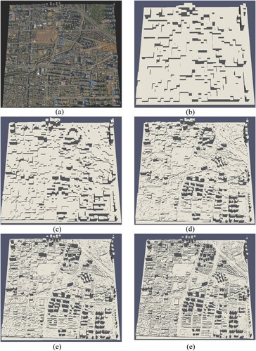
Raw data: The experiment was conducted in a local scenic area in Zhengzhou City, Henan Province, China, with a longitude range of ${113.688}^{\circ }\mathrm{E}$ to ${113.713}^{\circ }\mathrm{E}$ and latitude range of ${34.757}^{\circ }\mathrm{E}$ to ${34.777}^{\circ }\mathrm{E}$. The area covered approximately 2.2 $\mathrm{km}$ × 2.2 km and had an altitude range of 60 m to 220 m. The raw data comprised a 3D model constructed using oblique photogrammetry technology, as shown in Figure 11(a). The urban-scene data were voxelized using grids of specified sizes to create voxel models, as shown in Figure 11(b)–(f), with grid sizes of 68 × 68 × 20 m, 34 × 34 × 10 m, 17 × 17 × 5 m, 8.5 × 8.5 × 2.5 m, and 4.25 × 4.25 × 2.5 m. The scale of grid selection depends on two factors: the accuracy of the scene data and the safe-area size (or position-error ellipse) of the UAV. For convenience, in the following discussion, the voxel models corresponding to Figure 11(b)–(f) are denoted as ${\mathrm{V}}_1\text{–}{\mathrm{V}}_5$. Note that the grid sets depicted in Figure 11(b)–(e) result from urban-entity voxelization and belong to the UAV-impassable area, whereas the rest of the grids in the map space correspond to the feasible domain for UAV path planning. Subsequent experiments focused on the construction of different types of grid maps for feasible-domain grid sets.

Figure 11. Scene-vector data and voxelized scene models at different levels. The map sizes of (b) – (e) are $32\times 32\times 8$, $64\times 64\times 16$, $128\times 128\times 32$, $256\times 256\times 64$, $512\times 512\times 128$, respectively. (a) Local city scenes of Zhengzhou (b) ${\mathrm{V}}_1$ (c) ${\mathrm{V}}_2$ (d) ${\mathrm{V}}_3$ (e) ${\mathrm{V}}_4$ (e) ${\mathrm{V}}_5$.

UAV data: Rotary-wing UAVs were used for the experiment because of their flexibility, smallness, and hovering ability, which make them better suited than fixed-wing UAVs for complex environments such as cities (Quan et al. 2020). Therefore, we did not consider flight constraints such as the minimum turning radius or maximum climb/dive angle. For a single UAV, the beginning and end points were randomly generated on the environment grid map; the straight-line distance between them was constrained to be greater than 1800 m.

4.2.2. Computational environment

The experiments were performed on a system running Windows 10 and Visual Studio 2019 with a hardware configuration that included an Intel (R) Core (TM) i7-10870H CPU @ 2.20 GHz with 32 GB RAM.

4.3. Environment-construction experiment

4.3.1. Experimental procedure

1. Passable-area grid-set generation: The complement of the corresponding map space for voxel scene models of different sizes was calculated to obtain the UAV-passable-area set, which was also a single-scale grid map (SGM).

2. Multi-scale grid map construction: The framed-octree grid map (FOGM) was constructed from the single-scale planning map using the method in Chen, Szczerba, and Uhran (1995); the FSEGM was constructed from the single-scale planning map using the proposed method.

3. Data statistics: The number of grids and border grids used to construct the passable area and the time required for map construction on different types of maps were calculated.

4.3.2. Experimental results

The grid maps constructed using the different methods in the representative case of voxel model $V_3$ are shown in Figure 12. The orange grid set represents the voxel model and the light-purple grid set represents the traversable area. Their intersection is empty, and their union covers the entire map space. The traversable area shown in Figure 12(a) is an SGM constructed using single-scale grids, whereas the traversable area in Figure 12(b) is an FOGM. The traversable area shown in Figure 12(c) is the FSEGM constructed using the proposed method. Table 2 lists the number of grids and border grids used to construct the traversable-area grid maps for ${\mathrm{V}}_1\text{–}{\mathrm{V}}_5$.

Figure 12. Illustration of different types of grid maps corresponding to ${\mathrm{V}}_3$: (a) SGM, (b) FOGM, and (c) FSEGM.

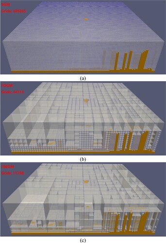
Table 2. Number of grids and border grids required to build each type of grid map for maps of different sizes.

	SGM	FOGM		FSEGM		Percentage Decrease
		$\mathrm{grid}$	$\mathrm{border}\mathrm{grid}$	$\mathrm{grid}$	$\mathrm{border}\mathrm{grid}$	$\mathrm{grid}$	$\mathrm{border}\mathrm{grid}$
${\mathrm{V}}_1$	4974	1684	4798	652	4630	61.3%	3.5%
${\mathrm{V}}_2$	46652	8544	39724	2707	36748	68.3%	7.5%
${\mathrm{V}}_3$	409265	44313	279025	11788	247729	73.4%	11.2%
${\mathrm{V}}_4$	3447814	213268	1752006	51481	1499686	75.9%	14.4%
${\mathrm{V}}_5$	28389549	998689	10206541	214309	8420469	78.5%	17.5%

The formulas used to calculate the percentage decrease in the grid number and border-grid number were respectively ${\displaystyle \frac{\mathrm{gri}{d}_{\mathrm{FOGM}}-\mathrm{gri}{d}_{\mathrm{FSEGM}}}{\mathrm{gir}{d}_{\mathrm{FOGM}}}\times 100\text{\%}}$ and ${\displaystyle \frac{\mathrm{framedGri}{d}_{\mathrm{FOGM}}-\mathrm{framedNu}{m}_{\mathrm{FSEGM}}}{\mathrm{framedNu}{m}_{\mathrm{FSEGM}}}\times 100\text{\%}}$.

4.3.3. Experimental analysis

(I) Figure 12 demonstrates that both FOGM and FSEGM can ensure identical construction accuracy as SGM in describing passable area. However, FSEGM requires considerably fewer grids than FOGM, because the scale-elastic discrete grid structure provides more flexible marking capabilities to satisfy the anisotropic scale requirements of voxels in different directions. Specifically, grids in FOGM can only be aggregated if they satisfy the octree aggregation relation (see Figure 12(b)), Conversely grids in FSEGM can also be aggregated if they satisfy the binary and quadtree aggregation relations (see Figure 12(c)). Therefore, the FSEGM can aggregate more grids than FOGM, which compresses the voxel model and significantly reducing the cost of storing environmental information.

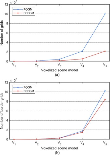
(II) Figure 13 and Table 2 show that the number of grids and border grids in both FOGM and FSEGM is proportional to the size of the base grid. As the size of the base grid decreases, the voxel model becomes more refined (see Figure 11). This increases in the number of grids and border grids. Moreover, the percentage decrease in grid number and the border-grid number increases as the size of the base grid decreases, with average values of 71.5% and 10.8%, respectively. This finding indicates that FSEGM can achieve an accurate representation of feasible areas with fewer grids and is more suitable than FOGM for path planning in large-range scenes.

Figure 13. Number of (a) grids and (b) border grids required to build FOGM and FSEGM for models ${\mathrm{V}}_1\text{–}{\mathrm{V}}_5$.

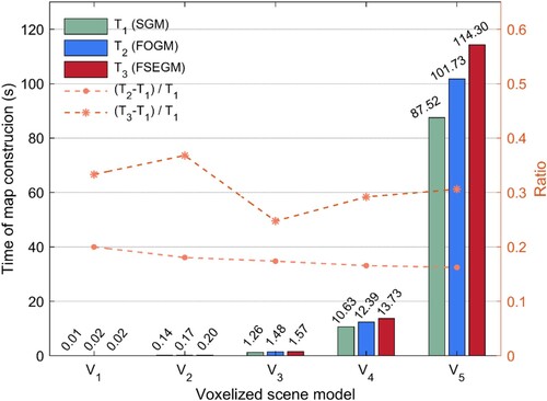
(III) As illustrated in Figure 14, both FOGM and FSEGM delay in building than SGM, with average increases of 17.6% and 30.9%, as indicated by the ratios ($\left(T_2-T_1\right)/T_1$ and $\left(T_3-T_1\right)/T_1$). When building the voxelized scene model, FSEGM required conducting aggregation operations in three separate directions (X, Y, Z) based on SGM. Conversely, FOGM only needed to perform one aggregation operation simultaneously in all three directions (X, Y, Z).

Figure 14. Time required to build SGM, FOGM and FSEGM for models ${\mathrm{V}}_1\text{–}{\mathrm{V}}_5$.

4.4. Planning-performance experiment

4.4.1. Experimental procedure

1. Map configuration: The SGM, FOGM, and FSEGM generated in the previous experiment were used as planning maps.

2. UAV data generation: Random UAV-path beginning and end-point coordinates were generated in the grid map.

3. Path planning: The standard A* algorithm was used for path planning in SGM, whereas both the standard A* algorithm and the multi-scale A* algorithm proposed in this study were used for path planning in FOGM and FSEGM.

4. Data statistics: The experiment was repeated 15 times, and the average values of indicators $c_1$ – $c_5$ were calculated under different conditions. Here, $c_1$ represents the number of nodes in the maintained list (OpenList) during the A* algorithm planning process; $c_2$ represents the number of nodes searched in the neighborhood; $c_3$ represents the number of nodes in the planned-path sequence, $c_4$ represents the actual length of the planned path, which is equal to the sum of the distances between the center points of adjacent grids in the planned-path node sequence; and $c_5$ represents the path-planning time.

4.4.2. Experimental results

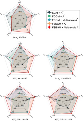
The results of path planning using different grid maps and path-planning algorithms are shown in Figure 15 for the representative case of voxel model $V_3$. The green paths in (a) and (b) represent the path-planning results in the SGM. The blue paths in (c) – (f) represent the planning results of FOGM; the corresponding multi-scale grid is shown in orange. The blue paths in (g) – (j) represent the planning results in the multiscale grid map based on the FSEGM; the corresponding multi-scale grid is shown in orange. The grids with red borders represent non-uniform subdivisions of dimensions; the borders are used to distinguish them from the grid nodes of the FOGM. The statistical results for the relevant indicators when different types of algorithms were used for path planning on maps of different scales are shown in Figure 16. Smaller values of each of the indicators $c_1\text{–}{c}_5$ correspond to better algorithm performance. For simplicity, the coordinate axes in Figure 16 have been flipped for illustrative purposes.

Figure 15. Illustration of path planning results (left column: side view; right column: top view) for (a)(b) SGM + A*, (c)(d) FOGM + A*, (e)(f) FOGM + Multi-scale A*, (g)(h) FSEGM + A*, and (i)(j) FSEGM + Multi-scale A*.

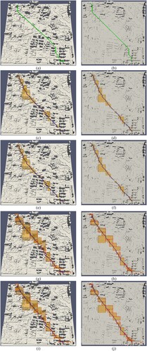
Figure 16. Statistical results of path planning indicators. $c_1$: number of maintained nodes; $c_2$: number of searched nodes; $c_3$: number of planned path nodes; $c_4$: length of planned path; $c_5$: path-planning time. The units of $c_4$ and $c_5$ are meters and milliseconds, respectively.

4.4.3. Experimental analysis

(I) Figure 15 demonstrates the successful application of the proposed multi-scale A* algorithm for path planning across various types of framed multi-scale maps, thereby confirming its feasibility.

(II) In maps of the same scale (see Figure 15), compared to the standard A* algorithm, the multi-scale A* algorithm proposed in this study effectively reduced $c_1$ and $c_2$, while ensuring the quality of path planning and improving planning efficiency. compared to the SGM and FOGM, FSEGM used in this study effectively reduced $c_2$ and $c_3$, while achieving a shorter planned path.

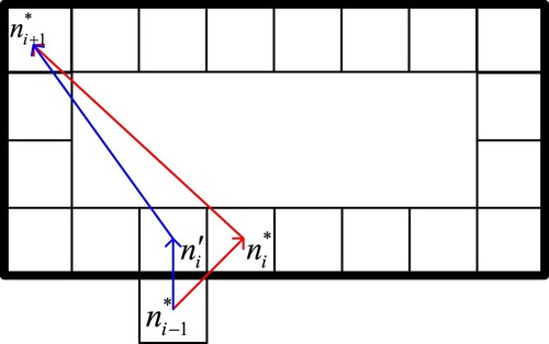
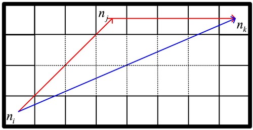
(III) For the planning-path length ($c_4$), the SGM + A* method resulted in significantly longer paths for ${\mathrm{V}}_2\text{–}{\mathrm{V}}_4$. This was primarily because the method was unable to utilize the long diagonal lines of the multiscale grid as planning paths, in contrast to multiscale methods. For instance, Figure 17 shows the path from node $n_i$ to node $n_k$. The red line represents the planned path obtained using the SGM + A* method, whereas the blue line represents the one obtained using either the A* algorithm or the multi-scale A* algorithm in FMGM (FOGM or FSEGM). It can be observed that both schemes successfully found the optimal paths considering their respective map representations. However, the planning algorithm based on FMGM could directly use as the planning-path length the Euclidean distance between the two border grids belonging to the same multi-scale grid, whereas SGM could only use the diagonal distance between them. Consequently, the SGM + A* method produced significantly longer paths.

Figure 17. Illustration of the planning length gap. Thick solid line: Node in FMGM (FOGM or FSEGM); Thin solid line: border grids for the node; Dashed line: Aggregated single-scale grid in the node. The red line indicates the optimal path from $n_i$ to $n_k$ planned in SGM. The blue line indicates the optimal path from $n_i$ to $n_k$ planned in FMGM.

(IV) The factors that affected the path-planning time ($c_5$) were primarily the number of maintained nodes ($c_1$) and search nodes ($c_2$). For the multi-scale A* algorithm, the time required for pruning calculations and neighborhood calculations for the multi-scale map should also be considered.

(V) For maps of different scales, different types of grid maps and planning algorithms had their advantages and disadvantages, and there was no absolute advantageous algorithm. Specifically, (1) In small-scale maps (such as ${\mathrm{V}}_1$ and ${\mathrm{V}}_2$), the path-planning time was relatively short, and the negative impact of the pruning-calculation time on the planning efficiency was greater for the multi-scale A* algorithm than the positive impact of the improved $c_1$ and $c_2$ indicators; therefore, the multi-scale A* algorithm is not suitable for such maps. Similarly, the neighborhood-calculation time caused by using a multi-scale map for planning has a relatively large impact; hence, the framed multi-scale map is not suitable for planning, and SGM + A* has higher planning efficiency in small-scale maps. (2) In medium-to-large-scale maps (such as ${\mathrm{V}}_3$, ${\mathrm{V}}_4$, ${\mathrm{V}}_5$), as the path-planning problem becomes more complex, the impact of the pruning-calculation time gradually decreases. Comparing Figure 15(c)–(e), it can be seen that for the same map structure, using the multi-scale A* algorithm was superior to using the A* algorithm overall. In this case, the primary factors affecting planning efficiency were $c_1$ and $c_2$. Therefore, the multi-scale A* algorithm is more suitable for maps of medium to large-scale. (3) In large-scale maps (such as ${\mathrm{V}}_4$, and ${\mathrm{V}}_5$), the structure of the grid map has a more significant impact on planning efficiency. Because the FSEGM has fewer grids and border grids, the number of nodes maintained and searched during path planning is relatively small, increasing planning efficiency. Therefore, the FSEGM is more suitable for path planning on large-scale maps.

5. Conclusion

This study proposes a multi-scale map-construction method using a scale-elastic discrete grid structure. The map constructed by this method solves the problem of the large number of nodes and heavy memory usage required by single-scale maps. It also solves the problem of the limited aggregation capability of existing tree-based multi-scale grid maps used to represent anisotropic large-scale scenes. Based on this method, a multi-scale A* algorithm is proposed; it prunes the number of nodes expanded in the neighborhood, reducing the number that must be maintained while ensuring optimality and improving path planning efficiency. Thus, it is suitable for path planning needs in large-range maps. The experiments indicate that (1) compared with the FOGM, the FSEGM constructed in this study can effectively reduce the number of grids and border grids, with average reductions of 71.5% and 10.8%, respectively, and larger reductions for larger map sizes; (2) compared with the standard A* algorithm, the multi-scale A* algorithm proposed in this study can effectively reduce the number of nodes searched and expanded in the neighborhood while ensuring the consistency of the planned path. Using the proposed method can effectively improve path-planning efficiency in large-range and complex scenes.

The map-construction and multi-scale path-planning methods studied in this paper can be combined with the framework we studied earlier for efficient multi-UAV path planning in complex, large-range urban scenes (Sun et al. 2023). A detailed discussion of this topic is presented in a separate publication.

Disclosure statement

No potential conflict of interest was reported by the author(s).

Data availability statement

The data that support the findings of this study are available at https://www.scidb.cn/anonymous/N2JJUnZh.

Additional information

Funding

This work was supported by the Program of Song Shan Laboratory (included in the Management of Major Science and Technology Program of Henan Province) under grant number 221100211000-03, the Natural Science Foundation of Henan Province under grant number 212300410096, and the National Key Research and Development Program of China under grant number 2018YFB0505304.

References

- Bailey ,James, Craig Tovey, Tansel Uras, Sven Koenig, and Alex Nash. 2015. “Path Planning on Grids: The Effect of Vertex Placement on Path Length.” Proceedings of the AAAI Conference on Artificial Intelligence and Interactive Digital Entertainment 11 (1): 108–114. https://doi.org/10.1609/aiide.v11i1.12808.
- Chen, Jinchao, Chenglie Du, Ying Zhang, Pengcheng Han, and Wei Wei. 2021. “A Clustering-Based Coverage Path Planning Method for Autonomous Heterogeneous UAVs.” IEEE Transactions on Intelligent Transportation Systems 23 (12): 25546–25556. https://doi.org/10.1109/TITS.2021.3066240.
- Chen, Jianhua, Xu Liu, Bingqian Wang, and Jian Lu. 2023. “A Clipping Algorithm for Real-Scene 3D Models.” International Journal of Digital Earth 16 (1): 464–485. https://doi.org/10.1080/17538947.2022.2159079.
- Chen, D. Z., R. J. Szczerba, and J. J. Uhran. 1995. “Planning Conditional Shortest Paths through an Unknown Environment: A Framed-Quadtree Approach.” Proceedings 1995 IEEE/RSJ International Conference on Intelligent Robots and Systems. Human Robot Interaction and Cooperative Robots 3: 33–38.
- Chen, D. Z., R. J. Szczerba, and J. J. Uhran. 1997. “A Framed-Quadtree Approach for Determining Euclidean Shortest Paths in a 2-D Environment.” IEEE Transactions on Robotics and Automation 13 (5): 668–681. https://doi.org/10.1109/70.631228.
- Cormen, T. H., C. E. Leiserson, R. L. Rivest, and Clifford Stein. 2022. Introduction to Algorithms. Cambridge, MA, USA: MIT Press.
- Daniel, K., A. Nash, S. Koenig, and A. Felner. 2010. “Theta*: Any-Angle Path Planning on Grids.” Journal of Artificial Intelligence Research 39 (October): 533–579. https://doi.org/10.1613/jair.2994.
- Gibb, Robert G., Matthew B.J. Purss, Zoheir Sabeur, Peter Strobl, and Tengteng Qu. 2022. “Global Reference Grids for Big Earth Data.” Big Earth Data 6 (3): 251–255. https://doi.org/10.1080/20964471.2022.2113037.
- Han, Bing, Tengteng Qu, Xiaochong Tong, Jie Jiang, Sisi Zlatanova, Haipeng Wang, and Chengqi Cheng. 2022. “Grid-Optimized UAV Indoor Path Planning Algorithms in a Complex Environment.” International Journal of Applied Earth Observation and Geoinformation 111:102857. https://doi.org/10.1016/j.jag.2022.102857.
- Harabor, Daniel Damir, Alban Grastien, Dindar Öz, and Vural Aksakalli. 2016. “Optimal Any-Angle Pathfinding in Practice.” Journal of Artificial Intelligence Research 56:89–118. https://doi.org/10.1613/jair.5007.
- Hauer, Florian, Abhijit Kundu, James M. Rehg, and Panagiotis Tsiotras. 2015. “Multi-Scale Perception and Path Planning on Probabilistic Obstacle Maps.” 2015 IEEE International Conference on Robotics and Automation (ICRA), 4210–4215.
- Hormazábal, Nicolás, Antonio Díaz, Carlos Hernández, and Jorge Baier. 2021. “Fast and Almost Optimal Any-Angle Pathfinding Using the 2k Neighborhoods.” Proceedings of the International Symposium on Combinatorial Search 8 (1): 139–143. https://doi.org/10.1609/socs.v8i1.18442.
- ISO 19170-4. 2023. Geographic Information – Discrete Global Grid Systems Specifications – Part 4: Axis-Aligned DGGS RS. https://committee.iso.org/sites/tc211/home/projects/projects—complete-list/iso-19170-4.html.
- Ivanov, Rosen. 2018. “An Algorithm for On-the-Fly K Shortest Paths Finding in Multi-Storey Buildings Using a Hierarchical Topology Model.” International Journal of Geographical Information Science 32 (12): 2362–2385. https://doi.org/10.1080/13658816.2018.1510126.
- Jordan, S., J. Moore, S. Hovet, J. Box, J. Perry, K. Kirsche, D. Lewis, and Z. T. H. Tse. 2018. “State-of-the-art technologies for UAV inspections.” IET Radar, Sonar & Navigation 12 (2): 151–164. https://doi.org/10.1049/iet-rsn.2017.0251.
- Lei, Yi, Xiaochong Tong, Tengteng Qu, Chunping Qiu, Dali Wang, Yuekun Sun, and Jiayi Tang. 2022. “A Scale-Elastic Discrete Grid Structure for Voxel-Based Modeling and Management of 3D Data.” International Journal of Applied Earth Observation and Geoinformation 113:103009. https://doi.org/10.1016/j.jag.2022.103009.
- Li, Y., W. Zhao, and Z. Zhou. 2014. “An Accelerated Method for Multiscale Path Planning.” Information and Control 43 (2): 211–216. https://doi.org/10.3724/SP.J.1219.2014.00211.
- Liu, Tao, Ruiqi Shen, Zhengling Lei, Yuchi Huo, Jiansen Zhao, and Xiaogang Xu. 2022. “Wind Resistance Aerial Path Planning for Efficient Reconstruction of Offshore Ship.” International Journal of Digital Earth 15 (1): 1881–1904. https://doi.org/10.1080/17538947.2022.2140852.
- Namdari, M. H., S. R. Hejazi, and M. Palhang. 2016. “Cornered Quadtrees/Octrees and Multiple Gateways Between Each Two Nodes; A Structure for Path Planning in 2D and 3D Environments.” 3D Research 7 (2): 1–18. https://doi.org/10.1007/s13319-016-0092-9.
- Nelson, Erik, Micah Corah, and Nathan Michael. 2018. “Environment Model Adaptation for Mobile Robot Exploration.” Autonomous Robots 42 (2): 257–272. https://doi.org/10.1007/s10514-017-9669-2.
- Pai, D. K., and L.-M. Reissell. 1998. “Multiresolution Rough Terrain Motion Planning.” IEEE Transactions on Robotics and Automation 14 (1): 19–33. https://doi.org/10.1109/70.660835.
- Pun-Cheng, L. S. C., M. Y. F. Tang, and I. K. L. Cheung. 2007. “Exact Cell Decomposition on Base Map Features for Optimal Path Finding.” International Journal of Geographical Information Science 21 (2): 175–185. https://doi.org/10.1080/13658810600852206.
- Quan, Lun, Luxin Han, Boyu Zhou, Shaojie Shen, and Fei Gao. 2020. “Survey of UAV Motion Planning.” IET Cyber-Systems and Robotics 2 (1): 14–21. https://doi.org/10.1049/iet-csr.2020.0004.
- Radmanesh, Mohammadreza, Manish Kumar, Paul H. Guentert, and Mohammad Sarim. 2018. “Overview of Path-Planning and Obstacle Avoidance Algorithms for UAVs: A Comparative Study.” Unmanned Systems 06 (02): 95–118. https://doi.org/10.1142/S2301385018400022.
- Rivera, Nicolás, Carlos Hernández, Nicolás Hormazábal, and Jorge A. Baier. 2020. “The 2^k Neighborhoods for Grid Path Planning.” Journal of Artificial Intelligence Research 67:81–113. https://doi.org/10.1613/jair.1.11383.
- Sun, Yuekun, He Li, Xiaochong Tong, Yi Lei, Dali Wang, Congzhou Guo, Jiayi Tang, and Yanfa Shang. 2023. “A Multi-Unmanned Aerial Vehicle Fast Path-Planning Method Based on Non-Rigid Hierarchical Discrete Grid Voxel Environment Modeling.” International Journal of Applied Earth Observation and Geoinformation 116:103139. https://doi.org/10.1016/j.jag.2022.103139.
- Szczerba, Robert J., Danny Z. Chen, and John J. Uhran. 1998. “Planning Shortest Paths among 2D and 3D Weighted Regions Using Framed-Subspaces.” The International Journal of Robotics Research 17 (5): 531–546. https://doi.org/10.1177/027836499801700505.
- Tanzmeister, Georg, Martin Friedl, Dirk Wollherr, and Martin Buss. 2014. “Efficient Evaluation of Collisions and Costs on Grid Maps for Autonomous Vehicle Motion Planning.” IEEE Transactions on Intelligent Transportation Systems 15 (5): 2249–2260. https://doi.org/10.1109/TITS.2014.2313562.
- Tsatcha, Dieudonné, Éric Saux, and Christophe Claramunt. 2014. “A Bidirectional Path-Finding Algorithm and Data Structure for Maritime Routing.” International Journal of Geographical Information Science 28 (7): 1355–1377. https://doi.org/10.1080/13658816.2014.887087.
- Tsouros, Dimosthenis C., Bibi Stamatia, and Panagiotis G. Sarigiannidis. 2019. “A Review on UAV-Based Applications for Precision Agriculture.” Information 10 (11): 349. https://doi.org/10.3390/info10110349.
- Wang, Wenxin, Bin Jiang, Jian Yang, and Chao Li. 2021. “Research on UAV Application in Mountain Anti-Terrorism Combat.” Journal of Physics: Conference Series 1792 (1): 012079. https://doi.org/10.1088/1742-6596/1792/1/012079.
- Xie, Ronglei, Zhijun Meng, Lifeng Wang, Haochen Li, Kaipeng Wang, and Zhe Wu. 2021. “Unmanned Aerial Vehicle Path Planning Algorithm Based on Deep Reinforcement Learning in Large-Scale and Dynamic Environments.” IEEE Access 9:24884–24900. https://doi.org/10.1109/ACCESS.2021.3057485.
- Xu, Minrui, Jiajie Xu, Rui Zhou, Jianxin Li, Kai Zheng, Pengpeng Zhao, and Chengfei Liu. 2023. “Empowering A* Algorithm with Neuralized Variational Heuristics for Fastest Route Recommendation.” IEEE Transactions on Knowledge and Data Engineering 35 (10): 10011–10023. https://doi.org/10.1109/TKDE.2023.3269084.
- Yan, Jinjin, Sisi Zlatanova, and Abdoulaye Diakité. 2021. “A Unified 3D Space-Based Navigation Model for Seamless Navigation in Indoor and Outdoor.” International Journal of Digital Earth 14 (8): 985–1003. https://doi.org/10.1080/17538947.2021.1913522.
- Yoon, Sangyol, Sung-Eui Yoon, Unghui Lee, and David Hyunchul Shim. 2015. “Recursive Path Planning Using Reduced States for Car-Like Vehicles on Grid Maps.” IEEE Transactions on Intelligent Transportation Systems 16 (5): 2797–2813. https://doi.org/10.1109/TITS.2015.2422991.
- Zhang, Songyi, Zhiqiang Jian, Xiaodong Deng, Shitao Chen, Zhixiong Nan, and Nanning Zheng. 2022. “Hierarchical Motion Planning for Autonomous Driving in Large-Scale Complex Scenarios.” IEEE Transactions on Intelligent Transportation Systems 23 (8): 13291–13305. https://doi.org/10.1109/TITS.2021.3123327.
- Zhang, Han-Ye, Wei-Ming Lin, and Ai-Xia Chen. 2018. “Path Planning for the Mobile Robot: A Review.” Symmetry 10:450. https://doi.org/10.3390/sym10100450.