Extreme environmental forcing on the container ship SS El Faro

ABSTRACT

The sinking of the cargo ship SS El Faro is investigated by providing a comprehensive analysis of the wind, wave and ocean currents associated with Hurricane Joaquin. Using state-of-the-art reanalyses the event is assessed in high resolution and from a long-term climate perspective. The last known location of the SS El Faro was in the north-west eye-wall of Hurricane Joaquin when it was a category four major Hurricane. The maximum individual wave height in this region was over 10 m and the Benjamin-Feir index was 0.69 indicating a high likelihood of rogue waves. As the vessel tried to outrun the hurricane it was continually impacted by strong wind and waves on its port side. This was compounded with flooding that caused a starboard list which likely eventually caused the vessel to sink.

KEYWORDS:

• Extreme waves
• hurricanes
• shipping
• ERA5
• HYCOM

1. Introduction

The International Convention for the Safety of Life at Sea (SOLAS) ensures safety standards are set in the construction, equipment and operation of merchant ships. The risks posed to a vessel during a voyage include: shifting cargo; running aground; collision and encountering inclement weather. An example of how shifting cargo can affect ship stability occurred with the vessel M.V. Hui Long. Munro and Mohajerani (2016) describe how liquefaction of the wet granular cargo occurred which altered the stability of the vessel and ultimately caused it to sink. An example of a ship running aground is the Costa Concordia cruise ship which capsized after striking a submerged rock off the coast of Isola del Giglio, Italy in 2012. A recent collision event which got international attention was the United States Navy destroyer USS Fitzgerald and a Philippine-flagged container ship off the coast in Japan in Summer 2017.

It is estimated that about one third of major ship accidents are associated with inclement weather (Toffoli et al. 2005). There have been multiple cases of vessels being sunk or damaged by very extreme sea states as is given in Cardone et al. (2015); Heij and Knapp (2015). Extra-tropical cyclones in the North Atlantic often cause extreme waves (Breivik et al. 2014; Bell et al. 2017) because of a ‘trapped fetch’, where a weather system is moving at the same speed as the group velocity of the waves and therefore providing the waves with continual forcing for growth. This situation caused the sinking of the fishing vessel Andrea Gail which was made famous in the movie ‘the perfect storm’. Extratropical cyclones pose a serious risk to vessels due to their size and localised strong winds (Gyakum 1983). Another factor which is a risk to container ships is parametric rolling in stormy seas (France et al. 2003). This is where large container vessels encounter head-on seas with a resonant wave period resulting in large roll angles that are coupled with significant pitch motions.

Hurricanes also pose an adverse risk to vessels as was the case with M. V. Derbyshire which was sunk by Typhoon Orchid in September 1980 (Faulkner 1998). Hurricanes are known to generate extreme waves (Curcic et al. 2016) and the waves are often multi-directional and short-crested. Fedele et al. (2017) found that the possibility the SS El Faro encountered a rogue wave in hurricane Joaquin was high at 1/130 in a 50-minute window using Higher-Order Spectral simulations.

Ocean wave period plays a role in determining wave steepness and therefore the likelihood of a rogue wave occurring. This was the case in the North Sea in December 2012 where 19 rogue waves occurred during a storm (Gibson et al. 2014; Bell et al. 2017). Ocean currents also influence wave behaviour both on the large scale and for individuals waves (Ardhuin et al. 2017). Strong ocean currents in the Agulhas are known to modify the height and shape of ocean waves causing extreme sea states which pose a risk in a main shipping route (Quilfen et al. 2018). It is therefore important to take into consideration wind, wave and currents when understanding the forces acting on a ship (Bell and Kirtman 2018).

The mechanism by which a vessel sinks in rough weather conditions is determined by a combination of environmental forcing (mostly wind and waves) and ship hydrodynamics. Each ship, by design, responds differently to various wave groups (i.e. significant wave height, wave periods and directions). These are determined by response amplitude operators (RAO; Cattrell et al. 2018). Unfortunately, the RAOs are not available for the SS El Faro hence this manuscript focusses on the environmental conditions that the vessel experienced. The increased resistance to a ship’s maneuverability from wind and waves also plays a part in the risk of vessel sinking during inclement weather. When a storm is approaching and the situation deteriorates the vessel can lose speed based on the environmental forcing, the hull, engine and propeller characteristics (Luo et al. 2016). This in turn limits the ability of the ship to outrun the storm.

The purpose of this study is to determine the evolution of the environmental conditions which led to the sinking of SS El Faro. There has only been one study pertaining to extreme waves during Hurricane Joaquin. Fedele et al. (2017) focused on the role of extreme waves in the sinking of the vessel but did not investigate the role of wind and currents. In our study, we use state-of-the-art reanalyses datasets to assess the wind, wave and currents associated with Hurricane Joaquin and the environmental forcing along the SS El Faro’s final transit.

The layout of this paper is as follows. The SS El Faro event is explained in Section 2. The data and parameters are described in Section 3. Validation of the reanalyses and the environmental conditions of the event are given in Section 4. A discussion is provided in Section 5 and lastly the conclusions are given in Section 6.

2. The SS El Faro

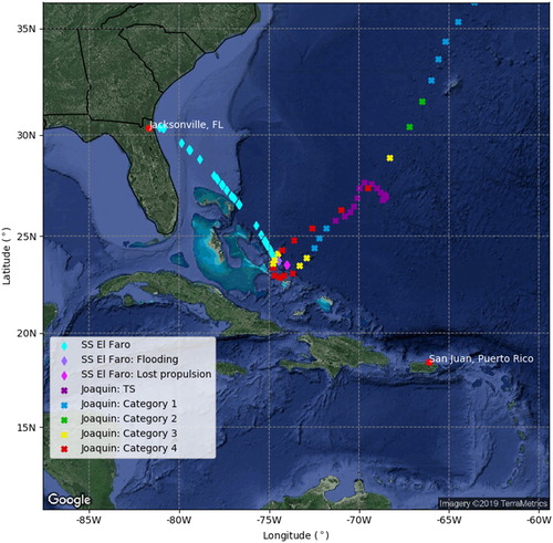
The SS El Faro is a container ship which ferried supplies between the United States and Puerto Rico. During a voyage in September 2015 SS El Faro encountered Hurricane Joaquin (Figure 1) and communications were lost. On the 31st of October the United States Navy Ship Apache identified the location of the sunken vessel. It was not until August 2016 that the Voyage Data Recorder (VDR) was recovered which contained information of the vessels position, date and time; engine information and audio from the bridge. This information was used in the National Transportation Safety Board’s (NTSB) investigation which concluded in December 2017. The NTSB criticised the captain’s decision to advance into the oncoming storm and noted he had relied on outdated weather information. It found flooding occurred in a cargo hold from an undetected open scuttle which caused a starboard list. This in turn affected oil levels in the engine room and the vessel lost propulsion (NTSB 2017).

Figure 1. Spatial map showing the known positions of SS El Faro and Hurricane Joaquin. The light blue diamond denotes positions of the vessel; the purple diamond denotes positions after flooding occurred; the pink diamond denotes positions after the vessel lost propulsion. The crosses show positions of Joaquin and the colour denotes the intensity: purple when Joaquin was a tropical storm; blue when Joaquin was a category 1 Hurricane; green when Joaquin was a category 2 Hurricane; yellow when Joaquin was a category 3 major Hurricane; red when Joaquin was a category 4 major Hurricane. The locations of Jacksonville, FL and San Juan, Puerto Rico are labelled as red circles. Image taken from Google.

3. Data and Methodologies

3.1. SS El Faro automatic identification system

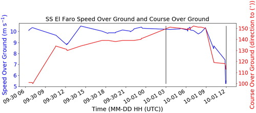
The SS El Faro ship data is provided by the NTSB’s investigation (https://dms.ntsb.gov/pubdms/search/document.cfm?docID=447557&docketID=58116&mkey=92109). The Automatic Identification System (AIS) provides vessel position logs as well the speed over ground (SOG: speed relative to the surface of the earth), the course over ground (COG: direction of progress) and heading (direction the bow is pointing). The data starts at 2015-09-28T20:34:044 UTC when the vessel was in the port of Jacksonville, Florida. The last data point is at 2015-10-01T11:57:07 UTC to the Northeast of Acklins and Crooked Island, Bahamas.

Figure 2 provides the SOG and COG of the SS El Faro along its transit. The drop in SOG is notable at 2015-10-01T09:00:00 UTC associated with flooding onboard. The final drop in the vessels speed from 8 to 5 m s⁻¹ occurred at 2015-10-01T11:49:13 UTC, shortly before contact was lost with the vessel. Associated with the drop in the vessel’s speed was a change in the vessels heading. As the ship lost power the vessel was being turned towards the east and towards the Hurricane.

Figure 2. Speed over ground and course over ground of SS El Faro along its transit. The black vertical bars denote the time-period which is investigated in Figures 12–14 as well as Table 1.

3.2. IBTrACS

Hurricane Joaquin data are obtained from the International Best Track Archive for Climate Stewardship (IBTrACS; Knapp et al. 2010). This provides positional data of the Hurricane and wind strength at six-hourly time steps. IBTrACS provides the best observations of hurricanes using all available satellite and in-situ observations (Landsea and Franklin 2013). The data for Joaquin in IBTrACS originates from HURDAT (Hurricane Databases).

3.3. Global drifter program

Surface current speed measurements are obtained from drifter observations and the methodology is fully described in Laurindo et al. (2017). The data is obtained from undrogued and 15-m drogue Global Drifter Program (GDP) drifters. This dataset contains more than 29 million six-hour position and velocity estimates from February 1979 to June 2015. The data is provided at 0.25° spatial resolution. Laurindo et al. (2017) note that the ocean surface current climatology is well represented in this dataset compare to other climatologies derived from in-situ data, as well as when compared to altimeter-derived geostrophic velocity fields.

3.4. Globwave

The 10-m surface wind speed and significant wave height data are obtained from the Globwave project (Gavrikov et al. 2016; Queffeulou and Croizé-Fillon 2016) as representative of our best estimate of observed conditions. This dataset consists of a 23-year time-period (1991–2015) and uses data from nine altimeters: ERS-1&2, TOPEX-Poseidon, GEOSAT Follow-ON (GFO), Jason-1, Jason-2, ENVISAT, Cryosat and SARAL. Data is restricted to 2000–2015 to match the same period as the ERA5 data. An empirical function is applied to the backscatter (e.g. Sepulveda et al. 2015) to calculate surface wind speed and significant wave height. The data is corrected using co-located buoy measurements (Skandrani et al. 2004). In general, the altimeter data are close to observations with some biases of overestimating low wind speed and significant wave heights, as well as underestimating high wind speed and significant wave heights. The satellite track files have been interpolated to match the spatial resolution of ERA5. It should be noted that altimeter winds are assimilated into ERA5.

3.5. HYCOM

The HYbrid Coordinate Ocean Model (HYCOM) is an ocean model which is isopycnal in the open ocean, terrain following in shallow coastal regions and z-level coordinates in unstratified seas. Data is used from the latest version of the Global Ocean Forecasting System (GOFS) 3.1 which is the HYCOM model combined with the Navy Coupled Ocean Data Assimilation (NCODA) system (Cummings 2005; Cummings and Smedstad 2013). GOFS 3.1 has improved physics and a well resolved surface layer. The horizontal resolution is 0.08° in the tropics and the temporal frequency is three-hourly. The draft of SS El Faro was 12 m, therefore surface current data is integrated over the top 12 m. Studies have shown HYCOM generally captures most energetic and persistent features such as western boundary currents but is limited with some mesoscale features (Savage et al. 2015; Carvalho et al. 2019).

3.6. ERA5

3.6.1. IFS

The European Centre for Medium-Range Weather Forecasts (ECMWF) 5th Generation (ERA5) reanalysis is used to assess the wind and waves. ERA5 is based on the predictions of a weather forecast model (Integrated Forecast System (IFS) Cycle 41r2) constrained by assimilation of data. The horizontal resolution of the atmospheric component of ERA5 is 31 km (T639) and data are available hourly (C3S 2017). Eventually, this reanalysis will replace ERA-Interim (Dee et al. 2011) thus validation of ERA5 data is still ongoing. Studies point towards that the higher resolution provides an improved assessment of extreme weather events (Olauson 2018).

3.6.2. WAM

The ocean wave model, the Wave Assimilation Model (WAM) is coupled with the atmospheric model and they communicate through the Charnock parameter which determines the roughness of the sea surface. The ocean wave model has slightly coarser resolution at 40 km. It uses 24 directions and 30 frequencies. ERA5 outputs the two-dimensional spectrum at every grid point as well as integrated parameters. The derivation of the integral parameters is provided below.

3.6.2.1. Ocean wave integral parameters

The two-dimensional wave spectrum describes how wave energy is distributed as a function of frequency $f$ and direction θ at each grid point:(1) $F\left(f,\theta \right)$(1) The one-dimensional wave spectrum describes how wave energy is distributed in $f$ and is defined as:(2) $E\left(f\right)={\int }_0^{2\pi }F\left(f,\theta \right)d\theta$(2) Bulk parameters can be obtained from the spectrum using spectral moments with the nth momentum given as:(3) $m_n={\int }_0^{2\pi }{\int }_0^{\mathrm{\infty }}{f}^{n}F(f,\theta )dfd\theta$(3) The significant wave height $H_s$ is defined as:(4) $H_s=4\sqrt{m_0}$(4) Mean wave period $T_{m-1}$ is given as:(5) $T_{m-1}=\frac{m_{-1}}{m_0}$(5) Mean zero-crossing wave period $T_{m2}$ is defined as:(6) $T_{m2}=\sqrt{\frac{m_0}{m_2}}$(6) Peak wave period $T_p$ is defined as:(7) $T_p=\frac{1}{f^p},$(7) where $f^p$ is the peak frequency of the one-dimensional spectrum.

Mean wave direction ${\theta }_m$ is given in oceanographic form with direction the waves are travelling toward and 0° being true north. It is defined as:(8) ${\theta }_m=\arctan \left(\frac{{\int }_0^{2\pi }{\int }_0^{\mathrm{\infty }}\sin \left(\theta \right)F\left(f,\theta \right)dfd\theta }{{\int }_0^{2\pi }{\int }_0^{\mathrm{\infty }}\cos \left(\theta \right)F\left(f,\theta \right)dfd\theta }\right)$(8) Mean directional spread ${\sigma }_{\theta }$ has values between zero (uni-directional spectra) and $\sqrt{2}$ (uniform spectra) and is defined as:(9) ${\sigma }_{\theta }=\sqrt{2\left(1-\frac{{\int }_0^{2\pi }{\int }_0^{\mathrm{\infty }}\cos \left(\theta -\overline{{\theta }_f}\right)F\left(f,\theta \right)dfd\theta }{E}\right),}$(9) where $\overline{{\theta }_f}$ is the mean direction $\theta$ at frequency $f$:(10) $\overline{{\theta }_f}=\arctan \left(\frac{{\int }_0^{2\pi }\sin \left(\theta \right)F\left(f,\theta \right)d\theta }{{\int }_0^{2\pi }\cos \left(\theta \right)F\left(f,\theta \right)d\theta }\right)$(10)

3.6.2.2. Rogue wave parameters

Rogue waves are defined as induvial waves that are much larger than surrounding waves. One common simple metric is if an individual wave is twice as large as the significant wave height $H=2H_s.$ A spectra wave model cannot compute individual waves – therefore rogue waves – explicitly but it can indicate an increased probability of their existence. One approach in which this is possible is by relating the shape of the probability density function of the surface elevation to the mean sea-state as described by the two-dimensional frequency spectrum (Janssen 2003). In a normal sea-state the distribution of the surface elevation has a gaussian shape. However, under exceptional circumstances deviations from Normality may occur which indicates the waves are nonlinear and there is an increased probability of rogue waves (Tayfun 1980; Tayfun and Fedele 2007).

The deviations from Normality are measured in terms of the kurtosis of the sea surface elevation:(11) $C_4=\frac{⟨{\eta }^4⟩}{3m_0^2}-1,$(11) with $\eta$ as the surface elevation.

According to the theory of wave-wave interactions the kurtosis $C_4$ is related to the frequency spectrum by:(12) $\begin{array}{rl}{C}_4& =\frac{4g}{m_0^2}P\int T_{1,2,3,4}\sqrt{\frac{{\omega }_4}{{\omega }_1{\omega }_2{\omega }_3}}\\ & \frac{E_1{E}_2{E}_3}{{\omega }_1+{\omega }_2-{\omega }_3-{\omega }_4}d{\omega }_{1}d{\omega }_{2}d{\omega }_{3}d{\theta }_{1}d{\theta }_{2}d{\theta }_3,\end{array}$(12) where $g$ is acceleration due to gravity, $P$ is the Cauchy principal value, $\omega$ is the angular frequency, $T_{1,2,3,4}$ is a complicated function of the four wave numbers (k_n; Krasitskii 1990). ${\omega }_4$ is:(13) ${\omega }_4=\mathrm{\Omega }\left(k_4\right)=\sqrt{g\left|k_1+k_2-k_3\right|}$(13) However, for an operational wave model, defining $C_4$ using Equation (12), a six dimensional integral, is too computationally expensive (Cattrell et al. 2018). Rogue waves most likely occur when the spectrum is narrow banded. One can therefore make a narrow band approximation. Based on numerical simulations of the Nonlinear Schröndinger equation which follows from the narrow-band limit of the Zakharov equation (Zakharov 1968) a fit can be obtained giving the maximum of the kurtosis. The total kurtosis can be approximated as:(14) $C_4=\left(\frac{0.031}{{\delta }_{\theta }}\times \frac{\pi }{3\sqrt{3}}BF{I}^2\right)+\alpha {\epsilon }^2,$(14) with ${\delta }_{\theta }$ the relative width of the directional spectrum. $\text{BFI}$ is the Benjamin-Feir Index given by:(15) $\text{BFI}=\frac{\epsilon \sqrt{2}}{{\delta }_{\omega }},$(15) with ε the integral steepness parameter:(16) $\epsilon =\frac{k_0}{\sqrt{m_0}}$(16) and ${\delta }_{\omega }$ the relative width of the frequency spectrum. For deep water α = 6.

The skewness $C_3$ of the probability density function of the surface elevation is useful to quantify the contribution of bound waves to the deviations from Normality. It is given as:(17) $C_3=\sqrt{\frac{k_3^2}{72}},$(17) (18) $k_3^2=5\left(k_{30}^2+k_{03}^2\right)+9\left(k_{21}^2+k_{21}^2\right)+6\left(k_{30}{k}_{12}+k_{03}{k}_{21}\right)$(18) Where $k_n$ refers to the third-order cumulants of the of the joint probability density function of the surface elevation and its Hilbert transform (Janssen 2014): $k_{30}=3\epsilon$; $k_{03}=0.$; $k_{12}=0.$; $k_{21}=\left(k_{30}/3\right)=\epsilon$.

These parameters to describe the deviation from Normality can be used to come up with an expression for the expected maximum wave height $H_{\mathrm{m}\mathrm{a}\mathrm{x}}$. For a large number of independent wave groups $N$ and small $C_4$, $H_{\mathrm{m}\mathrm{a}\mathrm{x}}$ can be approximated as:(19) $⟨H_{\mathrm{m}\mathrm{a}\mathrm{x}}⟩=\sqrt{{\hat{z}}_0+\frac{\gamma }{2}+\frac{1}{2}\text{log}\left[1+C_4\left\{2{\hat{z}}_0\left({\hat{z}}_0-1\right)-\gamma \left(1-2{\hat{z}}_0\right)-\frac{1}{2}\left({\gamma }^2+\frac{{\pi }^2}{6}\right)\right\}\right]},$(19) where ${\hat{z}}_0$ is related to the number of independent wave groups $N$ (Janssen 2014):(20) ${\hat{z}}_0=\frac{1}{2}\text{log}\left(\frac{T_D}{T_p}\right),$(20) $T_D$ is the duration of the time series and γ is Euler’s constant (0.5772). The expected wave period associated with $H_{\mathrm{m}\mathrm{a}\mathrm{x}}$ ($T_{\mathrm{m}\mathrm{a}\mathrm{x}}$) can be computed using the joint probability of the normalised envelope $R$ and normalised period T:(21) $R=\frac{H_{\mathrm{m}\mathrm{a}\mathrm{x}}/2}{\sqrt{2m_0}},$(21) (22) $T=\frac{2\pi /\omega }{2\pi \left({\displaystyle \frac{m_0}{m_1}}\right)},$(22) (23) $p\left(R,T\right)=\frac{2}{v\sqrt{\pi }}\frac{R^2}{T^2}\text{exp}\left\{-R^2\left[1+\frac{1}{v^2}{\left(1-\frac{1}{T}\right)}^2\right]\right\},$(23) where $v$ is the width parameter (Longuet-Higgins 1983):(24) $v=\sqrt{\frac{m_2{m}_0}{m_1^2}-1}$(24) For a given normalised envelope height, wave period follows the conditional distribution of wave periods $p\left(T|R\right)=p\left(R,T\right)/p\left(R\right)$:(25) $p\left(T|R\right)=\frac{R}{v\sqrt{\pi }{T}^2}\text{exp}\left[-\frac{R^2}{v^2}{\left(1-\frac{1}{T}\right)}^2\right],$(25)

$T_{\mathrm{m}\mathrm{a}\mathrm{x}}$ becomes the normalised period multiplied by the expected value of the period:(26) $T_{\mathrm{m}\mathrm{a}\mathrm{x}}=\sqrt{2m_0}⟨\frac{R}{v\sqrt{\pi }}{\int }_{-\mathrm{\infty }}^{\mathrm{\infty }}\frac{1}{T}\text{exp}\left[-\frac{R^2}{v^2}{\left(1-\frac{1}{T}\right)}^2\right]\text{d}T⟩$(26)

Maximum steepness is defined as:(27) $S_{\mathrm{m}\mathrm{a}\mathrm{x}}=\frac{2\pi H_{\mathrm{m}\mathrm{a}\mathrm{x}}}{g{T}_{\mathrm{m}\mathrm{a}\mathrm{x}}^2}$(27)

4. Results

4.1. Model validation

It is important that any biases or limitations of the models used to investigate the environment conditions during the SS El Faro’s final voyage are clearly stated. In this section, we compare the spatial biases of the models climatologies with the best estimate of observed conditions.

4.1.1. HYCOM validation

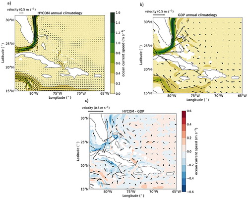
Figure 3 shows a comparison of the derived annual surface current climatology from HYCOM and that of in-situ drifters. Despite HYCOM having a higher spatial resolution than the drifter climatology it still simulates a weaker Florida current than observed. This has been noted in other studies. For example Duerr et al. (2012) found HYCOM under predicts mass transport at 27°N when compared to ADCP (Acoustic Doppler Current Profiler) measurements. The Antilles current, to the North of the Bahamas, is stronger in the drifter data compared to HYCOM by ∼0.25 m s⁻¹. In general, along the SS El Faro’s final transit the HYCOM simulation is remarkedly similar to the drifter data, especially east of 75°W.

Figure 3. Annual surface current speed and direction climatology for the period 2000–2015. (a) HYCOM; (b) GDP; (c) HYCOM minus GDP.

4.1.2. ERA5 10-m wind speed validation

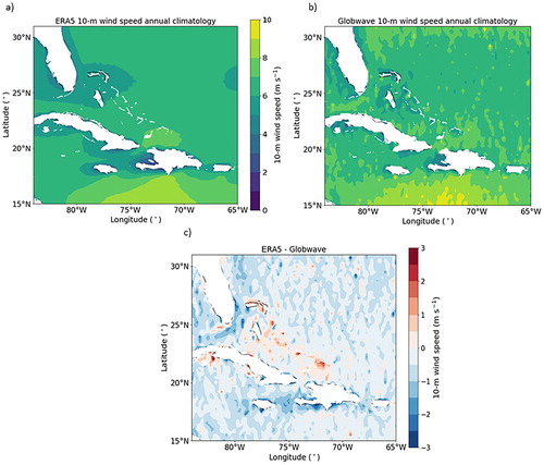
The Globwave annual 10-m wind speed climatology (Figure 4(b)) shows the altimeter tracks in the interpolated dataset and is demonstrable of a limitation of using satellite altimeter data. However, the altimeter data can distinguish large-scale features such as stronger wind speed around 15°N, 73°W and weaker wind speed to the west of Haiti. The 10-m wind speed simulated by ERA5 compares well to Globwave with most of the biases within −0.5–0.5 m s⁻¹. ERA5 wind speeds are slightly weaker in generally compared to Globwave although altimeters generally overestimate low wind speeds. The 10-m wind speed is stronger in ERA5 around the Caribbean Islands, but it is hard to validate altimeter data in coastal regions. In the region of the vessel route from Jacksonville to Puerto Rico ERA5 10-m wind speed is in good agreement with Globwave.

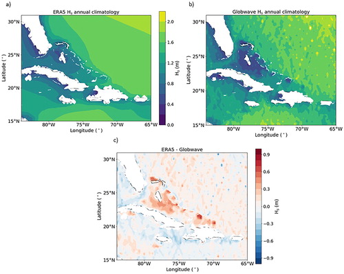
Figure 4. Annual 10-m wind speed climatology for the period 2000–2015. (a) ERA5; (b) Globwave; (c) ERA5 minus Globwave.

4.1.3. ERA5 significant wave height validation

ERA5 $H_s$ is in good agreement with Globwave (Figure 5(c)). The $H_s$ in most of the region in the south-west North Atlantic is close to the altimeter measured $H_s$ with biases of −0.3 to 0.3 m. The smaller Caribbean islands are not well resolved in ERA5 and as a result the $H_s$ is higher than observed. Satellite tracks can be observed in the interpolated Globwave dataset but to a lesser extent than the wind field. However, these results indicate that ERA5 is a valid model choice for the case study of extreme conditions that caused the SS El Faro to sink.

Figure 5. Annual significant wave height climatology for the period 2000–2015. (a) ERA5; (b) Globwave; (c) ERA5 minus Globwave.

4.2. The environmental conditions during the SS El Faro’s final transit

4.2.1. Ocean currents

A spatial map of the surface current speed at the time of the SS El Faro’s known last location is shown in Figure 6(a). The red cross denotes the centre of Hurricane Joaquin and the purple triangle is the position of SS El Faro. There is a Hurricane wind field signature in the ocean surface current response showing cyclonic motion. Figure 6(b) shows the same time slice, 2015-10-01T12:00:00 UTC, but as an anomaly compared to the climatological mean. Current speeds were twice as fast compared to climatology during Hurricane Joaquin especially on the south side of the storm. The ocean current speed and direction the vessel encountered was mostly consistent during the transit (Figure 7). The current speed was generally low between 0.2 and 0.5 m s⁻¹ and the ocean current direction was unfavourable for the journey as the current was moving towards the west.

Figure 6. (a) HYCOM surface current speed and direction on 2015-10-01T12:00:00 UTC. The purple diamond is the last known position of SS El Faro given at 2015-10-01T11:56:07 UTC. The red cross is the location of Hurricane Joaquin on 2015-10-01T12:00:00 UTC. (b) HYCOM surface current speed and direction on 2015-10-01T12:00:00 UTC minus HYCOM climatology.

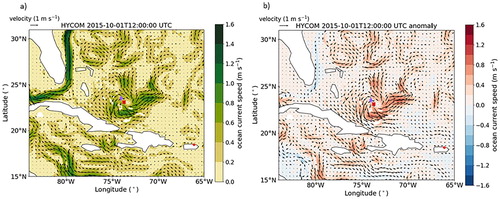
Figure 7. HYCOM ocean surface current speed and direction along the SS Faro track. The black vertical bars denote the time-period which is investigated in Figures 12–14 as well as Table 1.

4.2.2. Surface wind

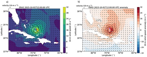
Figure 8 shows SS El Faro was located in the front right quadrant of Hurricane Joaquin where the highest winds speed are often found (Kossin et al. 2007). The vessel is also located in the eye wall which is the region with the most intense wind speeds. in ERA5, the strongest 10-m wind speed on 2015-10-01T12:00:00 UTC was 31 m s⁻¹. The observed 10-m wind speed at this time was 59 m s⁻¹ as given in IBTrACS. All reanalyses and to some extent operational global forecasts struggle to capture the strongest winds in hurricanes (Murakami 2014). It should be noted that the position of the hurricane given in ERA5 is in good agreement with observations.

Figure 8. (a) ERA5 10-m wind speed and direction on 2015-10-01T12:00:00 UTC. The description of purple diamond and the red cross are given in Figure 5. (b) ERA5 10-m wind speed and direction on 2015-10-01T12:00:00 UTC minus ERA5 climatology.

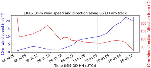
The time series of 10-m wind speed and wind direction at the location of SS El Faro is given in Figure 9. The SS El Faro experienced the largest winds speeds at approximately 2015-10-01T10:30:00 UTC, 90 min before contact was lost. The wind direction was constant at approximately north-easterly for about 18 h from 2015-09-30T18:00:00 UTC until 2015-10-01T10:30:00 UTC. This would have ensured the sea-state was well developed and the waves had a constant directional source of energy. The decrease in wind speed between 2015-09-30T11:00:00 UTC and 2015-09-30T12:00:00 UTC is associated with SS El Faro entering the eye of hurricane Joaquin.

Figure 9 . ERA5 10-m wind speed and direction along the SS El Faro track. The black vertical bars denote the time-period which is investigated in Figures 12–14 as well as Table 1.

4.2.3. Ocean waves

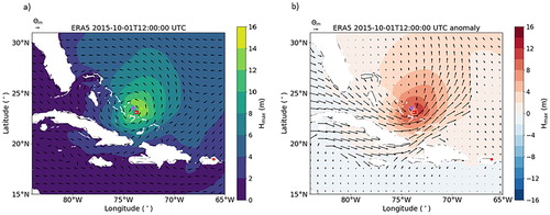
Figure 10(a) presents the maximum individual wave height $H_{\mathrm{m}\mathrm{a}\mathrm{x}}$ on 2015-10-01T12:00:00 UTC and Figure 10(b) shows how anomalous this period is compared to climatology. SS El Faro is located close the region of maximum $H_{\mathrm{m}\mathrm{a}\mathrm{x}}$ (the north-east quadrant) and is in a region where $H_{\mathrm{m}\mathrm{a}\mathrm{x}}$ is greater than 10 m. The maximum $H_{\mathrm{m}\mathrm{a}\mathrm{x}}$ is located to the north-east of the storm centre and the waves are smaller to the south-west as the islands dissipate the waves energy.

Figure 10. (a) ERA5 Maximum individual wave height and mean wave direction on 2015-10-01T12:00:00 UTC. The purple diamond and the red cross are given in Figure 5. (b) ERA5 Maximum individual wave height and mean wave direction on 2015-10-01T12:00:00 UTC minus ERA5 climatology.

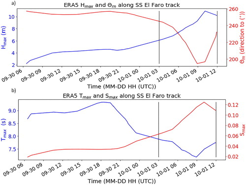
The mean wave direction ${\theta }_m$ the SS El Faro experienced shifted southward along the voyage as the Hurricane passed (Figure 11(a)). The wave period associated with the maximum individual wave height $T_{\mathrm{m}\mathrm{a}\mathrm{x}}$ got shorter as the Hurricane approached SS El Faro from 9.3 to 7.2 s (Figure 11(b)) and as a result the wave steepness increased.

Figure 11 . (a) ERA5 Maximum individual wave height and mean wave direction along the SS El Faro track. (b) ERA5 period corresponding to maximum individual wave height and wave steepness along SS El Faro track. The black vertical bars denote the time-period which is investigated in Figures 12–14 as well as Table 1.

4.2.4. Wave spectra and rogue waves

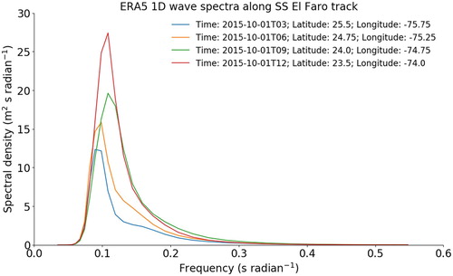
Wave energy increased as the SS El Faro continued its journey south-eastward. This can be seen in the one-dimensional wave spectra (Figure 12). The blue line gives the wave spectra integrated over all directions at the location of SS El Faro at 2015-10-01T03 UTC. At this time the wave field was almost fully developed with the peak wave energy at 0.1 s radian⁻¹. Throughout the next nine hours the wave energy increased and the spectra became more narrow banded. The peak of wave energy slightly shifted to shorter waves as the vessel got closer to the hurricane and therefore closer to the source of wind input.

Figure 12. One-dimensional Ocean wave frequency spectra along the SS El Faro track. Four time periods are shown leading up to the last known location of SS El Faro on 2015-10-01T11:56:07 UTC. The time, latitude and longitude for the spectra are given in the legend.

The two-dimensional wave spectra for the same location and time are displayed in Figure 13. The contours represent wave energy on a logarithmic scale. At 2015-10-01T03:00:00 UTC (Figure 13(b)) the wave energy is mostly travelling to the west and south-west. As the Hurricane neared, the wave energy backed and moved toward a southward direction. At the last known location, the waves became multi-directional and a secondary partition is apparent with some waves travelling north-westward. These can be seen in the directional spreading (${\sigma }_{\theta }$) which increased from 0.56 to 0.91 between 2015-10-01T09:00:00 and 2015-10-01T12:00:00 (Table 1).

Figure 13. Two-dimensional ocean wave spectra. Each panel (a–d) corresponds to a time, latitude and longitude given in Figure 12.

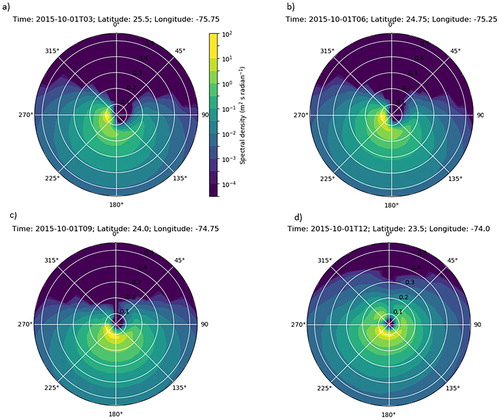
Table 1. Environmental parameters at the location of SS El Faro for the time periods 2015-10-01T03:00:00 UTC to 2015-10-01T12:00:00 UTC.

Time	1/10/2015 0300	1/10/2015 0600	1/10/2015 0900	1/10/2015 1200
Latitude (°)	25.5	24.8	24	23.5
Longitude (°)	−75.7	−75.3	−74.8	−74
SOG (m s^−1)	10.2	10.1	10.2	5.5
COG (° to)	151	149	150	113
Current speed (m s^−1)	0.19	0.21	0.41	0.38
Current direction (° to)	273	221	206	250
10-m wind speed (m s^−1)	10.4	14.3	19.3	20
10-m wind direction (° from)	75	87	86	24
$H_s$ (m)	3.3	3.9	4.9	5.2
$H_{max}$ (m)	6.3	7.4	9.4	10
$H_{max}/H_s$	1.91	1.90	1.92	1.92
${\theta }_m$ (° to)	241	227	195	234
$T_{max}$ (s)	7.7	7.5	7.2	7.7
$S_{\mathrm{m}\mathrm{a}\mathrm{x}}$	0.07	0.08	0.12	0.11
$T_{m-1}$ (s)	8.7	8.4	8	8.4
$T_{m2}$ (s)	6.6	6.5	6.3	6.9
$T_p$ (s)	10.7	10.1	9	9.3
${\sigma }_{\theta }$	0.49	0.52	0.56	0.91
$C_4$	0.02	0.02	0.04	0.05
$\text{BFI}$	0.4	0.41	0.61	0.69
$C_3$	0.03	0.04	0.06	0.06

Along with the wave energy increasing there was also an increased likelihood that rogue waves occurred. The wave spectral kurtosis ($C_4$), Benjamin-Feir Index ($\text{BFI}$) and wave spectral skewness ($C_3$) all increase during this period. The $\text{BFI}$, which represents the ratio between wave steepness and spectral bandwidth, is large at 0.69. As a comparison the $\text{BFI}$ was 0.24 during the Andrea rogue wave event (Fedele et al. 2016; Donelan and Magnusson 2017). The $C_4$ and $C_3$ values increase but only slightly over the period of nine hours. It can also be seen that $H_{\mathrm{m}\mathrm{a}\mathrm{x}}/H_s$ remains constant during this period at ∼1.9.

5. Discussion and conclusions

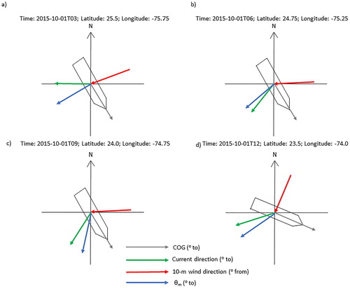
The evolution of the environmental forcing on the container ship SS El Faro during the final nine hours is presented in Figure 14. The transit from Jacksonville to San Juan has a COG of approximately 145°. The vessel experienced strong persistent winds on her port side as the captain made the decision to continue the journey and attempt to outrun the hurricane. This was compounded by the fact the hurricane had an unusually south-westerly track so the situation deteriorated over time. The red arrow is the 10-m wind speed direction which is almost perpendicular to the vessel throughout the time-period shown. This explains the starboard list of the vessel. The blue arrow is the mean wave direction (${\theta }_m$) and indicates that it mostly follows the wind except for 2015-10-01T09:00:00 where ${\theta }_m$ is southward and the 10-m wind direction is easterly. When the vessel lost power shortly before 2015-10-01T12:00:00 the environmental conditions caused the vessel to turn to the port side thus the angle of the wind to the COG was ∼90°. The 10-m wind speed, ${\theta }_m$ and current direction were all impacting the vessel’s port side. This is an extremely dangerous situation as the vessel’s roll is largest when wind and waves are perpendicular to the vessel’s heading. Once the vessel lost power it was unable to correct its position relative to the wind and waves. This meant there was a greater chance that the vessel was struck by a rouge wave. This hypothesis is strengthened when looking at parameters that represent the likelihood of rouge waves. The individual maximum wave height and the Benjamin-Feir Index were largest at the point in time and space of the last known location of the vessel.

Figure 14. SS El Faro course over ground associated with the time and locations given in Figure 12. The grey arrow indicates the course over ground; the green arrow denotes the ocean surface current direction. The red arrow shows the direction of the 10-m wind and the blue arrow denotes the mean wave direction.

As ERA5 is a spectra wave model it cannot provide information of individual wave heights as were provided in Fedele et al. (2017). Thus, it cannot be used to explicitly quantify the likelihood that a rogue wave sunk the SS El Faro. However, the study of Fedele et al. (2017) can be expanded upon using initial wave field conditions of ERA5 for Higher-Order pseudo-Spectral (HOS) simulations.

The models used in this study provide good agreement with observed datasets to represent the wind, wave and ocean current climatology of the Caribbean. GOFS 3.1 shows similar results with observed drifter data although HYCOM simulates the Florida current and Antilles current weaker than observed. This indicates that while HYCOM is a relative high-resolution ocean model with 1/12° grid spacing, higher resolution or improved physical parametrizations may be needed to accurately simulate the strength of Ocean boundary currents. The mean-state 10-m wind speed and significant wave height in ERA5 compared to altimeter measurements are mostly in good agreement. The difference is largest around the small Caribbean islands. This is not surprising as ERA5 is a global model and uses sub-grid parametrization to represent wave energy dissipations by islands smaller that a grid cell. It is an improvement over ERA-Interim but more research is needed in this space.

ERA5 simulated the maximum individual wave height $H_{\mathrm{m}\mathrm{a}\mathrm{x}}$ to be greater than 10 m at the last recorded location of SS El Faro which was in the north-west eye wall of Hurricane Joaquin. The wave period associated with the maximum individual wave height $T_{\mathrm{m}\mathrm{a}\mathrm{x}}$ decreased along the vessel’s voyage and the steepness increased. The coefficients of skewness and kurtosis increased and peaked after the vessel transmitted its last location. In addition, the Benjamin-Feir index increased to 0.69 indicating there was a high likelihood that rogue waves occurred.

A comprehensive analysis of the ocean current direction, 10-m wind direction and two-dimensional ocean wave spectrum respective to SS El Faro’s course over ground is portrayed. This provides qualitative information of the dynamic behaviour of the ship without the existence of the vessels RAOs (Ibrahim and Grace 2010). The strong persistent wind and waves on the vessels port side amplified the starboard list. This coupled with a high probability that rogue waves were present are what were likely to have caused the vessel to sink. An improved knowledge of ocean conditions caused by extreme weather can improve safety during vessel routing (Edwing 2018). This study demonstrates that HYCOM and ERA5 can be used further to understand the relationship between extreme environmental forcing and vessel safety.

Acknowledgements

The authors would like to thank the National Ocean Partnership Program for providing the HYCOM data and the European Center for Medium range Weather Forecasts for proving ERA5 data. We thank Milan Curcic for providing comments on an early draft of this manuscript. We thank the anonymous reviewers for their suggestions on ways to improve this manuscript. We thank the developers of the following open-source python packages: Xarray, Dask, Cartopy, Matplotlib, salem and cmocean.

Disclosure statement

No potential conflict of interest was reported by the authors.

Additional information

Funding

The authors acknowledge support from a National Oceanic and Atmospheric Administration award NA15OAR4320064 and an Office of Naval research award N6833516C0087.

References

- Ardhuin F, Gille ST, Menemenlis D, Rocha CB, Rascle N, Chapron B, Gula J, Molemaker J. 2017. Small-scale open ocean currents have large effects on wind wave heights. J Geophys Res Oceans. 122(6):4500–4517. doi: 10.1002/2016JC012413
- Bell RJ, Gray SL, Jones OP. 2017. North Atlantic storm driving of extreme wave heights in the North Sea. J Geophys Res Oceans. 122(4):3253–3268. doi: 10.1002/2016JC012501
- Bell R, Kirtman B. 2018. Seasonal forecasting of winds, waves and currents in the North Pacific. J Oper Oceanogr. 11:11–26.
- Breivik Ø, Aarnes OJ, Abdalla S, Bidlot J-R, Janssen PAEM. 2014. Wind and wave extremes over the world oceans from very large ensembles. Geophys Res Lett. 41(14):5122–5131. doi: 10.1002/2014GL060997
- C3S. 2017. ERA5: fifth generation of ECMWF atmospheric reanalyses of the global climate. Copernicus Climate Change Service Climate Data Store (CDS). https://cds.climate.copernicus.eu/cdsapp#!/home.
- Cardone VJ, Callahan BT, Chen H, Cox AT, Morrone MA, Swail VR. 2015. Global distribution and risk to shipping of very extreme sea states (VESS). Int J Climatol. 35(1):69–84. doi: 10.1002/joc.3963
- Carvalho JPS, Costa FB, Mignac D, Tanajura CAS. 2019. Assessing the extended-range predictability of the ocean model HYCOM with the REMO ocean data assimilation system (RODAS) in the South Atlantic. J Oper Oceanog. 1–11.
- Cattrell AD, Srokosz M, Moat BI, Marsh R. 2018. Can rogue waves be predicted using characteristic wave parameters? J Geophys Res Oceans. 123(8):5624–5636. doi: 10.1029/2018JC013958
- Cummings JA. 2005. Operational multivariate ocean data assimilation. Q J R Metereol Soc. 131(613):3583–3604. doi: 10.1256/qj.05.105
- Cummings JA, Smedstad OM. 2013. Variational data assimilation for the global ocean BT – data assimilation for atmospheric, oceanic and hydrologic applications (vol. II). Berlin: Springer Berlin Heidelberg.
- Curcic M, Chen SS, Özgökmen TM. 2016. Hurricane-induced ocean waves and stokes drift and their impacts on surface transport and dispersion in the Gulf of Mexico. Geophys Res Lett. 43(6):2773–2781. doi: 10.1002/2015GL067619
- Dee DP, Uppala SM, Simmons AJ, Berrisford P, Poli P, Kobayashi S, Andrae U, Balmaseda MA, Balsamo G, Bauer P, et al. 2011. The ERA-interim reanalysis: configuration and performance of the data assimilation system. Q J Roy Meteorol Soc. 137(656):553–597. doi: 10.1002/qj.828
- Donelan MA, Magnusson A-K. 2017. The making of the Andrea wave and other rogues. Sci Rep. 7:44124. doi: 10.1038/srep44124
- Duerr AES, Dhanak MR, Van Zweiten J. 2012. Utilizing the hybrid coordinate ocean model data for the assessment of the Florida current’s hydrokinetic renewable energy resource. Mar Technol Soc J. 46(5):24–33. doi: 10.4031/MTSJ.46.5.2
- Edwing RF. 2018. NOAA’s physical oceanographic real-time system (PORTS®). J Oper Oceanogr. 1–11.
- Faulkner D. 1998. An independent assessment of the sinking of the MV DERBYSHIRE. SNAME Trans. 106:59–103.
- Fedele F, Brennan J, Ponce de León S, Dudley J, Dias F. 2016. Real world ocean rogue waves explained without the modulational instability. Sci Rep. 6:27715. doi: 10.1038/srep27715
- Fedele F, Lugni C, Chawla A. 2017. The sinking of the El Faro: predicting real world rogue waves during Hurricane Joaquin. Sci Rep. 7:11188. doi: 10.1038/s41598-017-11505-5
- France WN, Levadou M, Treakle TW, Paulling JR, Michel RK, Moore C. 2003. An investigation of head-sea parametric rolling and its influence on container lashing systems. Mar Technol. 40(1):1–19.
- Gavrikov AV, Krinitsky MA, Grigorieva VG. 2016. Modification of Globwave satellite altimetry database for sea wave field diagnostics. Oceanology. 56(2):301–306. doi: 10.1134/S0001437016020065
- Gibson R, Christou M, Feld G. 2014. The statistics of wave height and crest elevation during the December 2012 storm in the North Sea. Ocean Dyn. 64(9):1305–1317. doi: 10.1007/s10236-014-0750-5
- Gyakum JR. 1983. On the evolution of the QE II storm. I: synoptic aspects. Mon Weather Rev. 111(6):1137–1155. doi: 10.1175/1520-0493(1983)111<1137:OTEOTI>2.0.CO;2
- Heij C, Knapp S. 2015. Effects of wind strength and wave height on ship incident risk: regional trends and seasonality. Transport Res D-TR E. 37:29–39. doi: 10.1016/j.trd.2015.04.016
- Ibrahim RA, Grace IM. 2010. Modeling of ship roll dynamics and its coupling with heave and pitch. Math Probl Eng. 2010:1–32. doi: 10.1155/2010/934714
- Janssen PAEM. 2003. Nonlinear four-wave interactions and freak waves. J Phys Oceanogr. 33:863–884. doi: 10.1175/1520-0485(2003)33<863:NFIAFW>2.0.CO;2
- Janssen PAEM. 2014. On a random time series analysis valid for arbitrary spectral shape. J Fluid Mech. 759:236–256. doi: 10.1017/jfm.2014.565
- Knapp KR, Kruk MC, Levinson DH, Diamond HJ, Neumann CJ. 2010. The international best track archive for climate stewardship (IBTrACS). Bull Amer Meteor Soc. 91(3):363–376. doi: 10.1175/2009BAMS2755.1
- Kossin JP, Knaff JA, Berger HI, Herndon DC, Cram TA, Velden CS, Murnane RJ, Hawkins JD. 2007. Estimating hurricane wind structure in the absence of aircraft reconnaissance. Weather Forecast. 22(1):89–101. doi: 10.1175/WAF985.1
- Krasitskii VP. 1990. Canonical transformation in a theory of weakly non-linear waves with a nondecay dispersion law. Sov Phys JETP. 71:921–927.
- Landsea CW, Franklin JL. 2013. Atlantic hurricane database uncertainty and presentation of a new database format. Mon Wea Rev. 141(10):3576–3592. doi: 10.1175/MWR-D-12-00254.1
- Laurindo LC, Mariano AJ, Lumpkin R. 2017. An improved near-surface velocity climatology for the global ocean from drifter observations. Deep Sea Res Part I. 124:73–92. doi: 10.1016/j.dsr.2017.04.009
- Longuet-Higgins MS. 1983. On the joint distribution of wave periods and amplitudes in a random wave field. Proc R Soc Lond. 389:241–258.
- Luo S, Ma N, Hirakawa Y. 2016. Evaluation of resistance increase and speed loss of a ship in wind and waves. J Ocean Eng Sci. 1(3):212–218. doi: 10.1016/j.joes.2016.04.001
- Munro MC, Mohajerani A. 2016. Liquefaction incidents of mineral cargoes on board bulk carriers. Adv Mater Sci Eng. 5219474:20.
- Murakami H. 2014. Tropical cyclones in reanalysis data sets. Geophys Res Lett. 41(6):2133–2141. doi: 10.1002/2014GL059519
- NTSB. 2017. Board meeting: October 2015 sinking of the cargo ship EL FARO in the Atlantic Ocean. https://www.ntsb.gov/news/events/Pages/2017-DCA16MM001-BMG.aspx.
- Olauson J. 2018. ERA5: the new champion of wind power modelling? Renewable Energ. 126:322–331. doi: 10.1016/j.renene.2018.03.056
- Queffeulou P, Croizé-Fillon D. 2016. Global altimeter SWH data set – September 2016.
- Quilfen Y, Yurovskaya M, Chapron B, Ardhuin F. 2018. Storm waves focusing and steepening in the Agulhas current: satellite observations and modeling. Remote Sens Environ. 216:561–571. doi: 10.1016/j.rse.2018.07.020
- Savage JA, Tokmakian RT, Batteen ML. 2015. Assessment of the HYCOM velocity fields during Agulhas return current cruise 2012. J Oper Oceanogr. 8(1):11–24.
- Sepulveda HH, Queffeulou P, Ardhuin F. 2015. Assessment of SARAL/AltiKa wave height measurements relative to Buoy, Jason-2, and Cryosat-2 data. Mar Geod. 38:449–465. doi: 10.1080/01490419.2014.1000470
- Skandrani C, Lefevre J-M, Queffeulou P. 2004. Impact of multisatellite altimeter data assimilation on wave analysis and forecast. Mar Geod. 27(3):511–533. doi: 10.1080/01490410490883496
- Tayfun MA. 1980. Narrow-band nonlinear sea waves. J Geophys Res. 85:1548–1552. doi: 10.1029/JC085iC03p01548
- Tayfun MA, Fedele F. 2007. Wave-height distributions and nonlinear effects. Ocean Eng. 34:1631–1649. doi: 10.1016/j.oceaneng.2006.11.006
- Toffoli A, Lefèvre JM, Bitner-Gregersen E, Monbaliu J. 2005. Towards the identification of warning criteria: analysis of a ship accident database. Appl Ocean Res. 27(6):281–291. doi: 10.1016/j.apor.2006.03.003
- Zakharov VE. 1968. Stability of periodic waves of finite amplitude on the surface of a deep fluid. J Appl Mech Tech Phys. 9:190–194. doi: 10.1007/BF00913182