Copernicus Ocean State Report, issue 6

Supplemental Material

References

CMEMS. 2016. Product quality strategy plan. Available from: https://marine.copernicus.eu/sites/default/files/CMEMS-PQ-StrategicPlan-v1.6-1_0.pdf.
Google Scholar
Le Traon PY, Reppucci A, Alvarez Fanjul E, Aouf L, Behrens A, Belmonte M, Bentamy A, Bertino L, Brando VE, Kreiner MB, et al. 2019. From observation to information and users: the copernicus marine service perspective. Front Mar Sci. 6:234. Available from: https://www.frontiersin.org/article/10.3389/fmars.2019.00234.
Web of Science ®Google Scholar
von Schuckmann K, Le Traon P-Y, Smith N, Pascual A, Brasseur P, Fennel K, Djavidnia S, Aaboe S, Fanjul EA, Autret E, et al. 2018. Copernicus marine service ocean state report. J Oper Oceanogr. 11(Suppl. 1):S1–S142. doi:10.1080/1755876X.2018.1489208.
Google Scholar

Chapter 2: Novel scientific analyses of the ocean state and its variability at various space and time

Section 2.1. Changes in extreme wind speeds over the global ocean

Authors: Rianne Giesen, Ad Stoffelen

Statement of main outcome: In 2020, the northern Atlantic experienced both a record-high number of intense tropical cyclones and several heavy storms at higher latitudes. On the other hand, tropical cyclone activity was reduced in the western Northern Pacific. To put these anomalies into a longer-term perspective, we use remotely sensed winds from a scatterometer over the period 2007–2020 to analyse extreme wind speeds over the global ocean, based on the 99th percentile. We compare the 2020 extreme winds to the 2007–2014 climatology and determine significant trends in extreme wind speeds. We find that the 2020 anomalies in the northern Atlantic and Pacific exceed the interannual variability observed over the period 2007–2019, but cannot be directly associated with a significant trend over 2007–2020. On the other hand, large positive extreme wind speed anomalies are found in the southern Indian Ocean, that are in line with steadily increasing extreme wind speeds in this region. Another large positive 2020 anomaly and 2007–2020 trend is observed in the tropical southern Pacific, east of the Solomon Islands. Predominantly negative 2020 anomalies and trends are detected in the southern Pacific Ocean and northwest of New Zealand. Compared to the extreme scatterometer winds, collocated reanalysis model winds are systematically lower and generally exhibit smaller trends.

Product table:

Table

2.1.1. Introduction

Storms are one of the most threatening natural hazards. Especially in densely populated coastal regions, the combination of high wind speeds, extreme waves, storm surges and heavy rainfall in storms causes severe damage and loss of lives (Bevere et al. Citation2020). In the tropical regions, the most extreme surface wind speeds occur, regularly reaching category 5 hurricane strengths with wind speeds above 250 km per hour or 70 m s⁻¹. At higher latitudes, extreme wind speeds are generally observed in low-pressure systems along mid-latitude storm tracks and in polar lows (Marseille et al. Citation2019). Apart from disastrous impacts on society, high wind speeds play an important role in atmosphere-ocean interaction, for instance through changes in the upper-ocean circulation and the exchange of momentum, heat and mass between the atmosphere and the ocean (Russell et al. Citation2021).

The year 2020 saw a record-breaking number of named tropical storms in the Atlantic (Bevere et al. Citation2020). Over the past four decades, the global proportion of intense tropical cyclones has likely increased (IPCC Citation2021). Future projections suggest with high confidence that peak wind speeds of intense tropical cyclones will increase with increased global warming (Knutson et al. Citation2020). On the other hand, there is medium confidence that the overall global frequency of tropical storms will remain unchanged or decrease (Collins et al. Citation2019). The future position and intensity of mid-latitude storm tracks are connected to changes in temperature gradients (Shaw et al. Citation2016). Since opposing effects occur, future projections have low confidence, particularly in the northern hemisphere (IPCC Citation2021). Projections for the southern hemisphere are more consistent and suggest a strengthening and southward contraction of the storm tracks (Russell et al. Citation2021).

Since in-situ observations of extreme wind speeds are rare, especially over the open ocean, satellite instruments are fundamental to monitor changes in extreme wind occurrence. Several decades of ocean surface wind measurements are available from active microwave radar instruments (scatterometers and altimeters) and passive microwave instruments (radiometers) (Bourassa et al. Citation2019). Scatterometers and radiometers measure contiguously in broad swaths of typically 1000 km wide and cover about a third of the earth surface in 12 h. Scatterometers provide surface vector winds up to 40 m s⁻¹ since 1992. Radiometers are not suitable for studying extreme wind statistics, because they poorly measure wind speed in rain conditions, which generally coincide with extreme winds. Past altimeters have tracks rather than swaths, and have much less reliable sampling of the wind extremes than scatterometers and radiometers. While homogenised ocean surface wind climate data records exist, differences among instruments and producers are large (Stoffelen et al. Citation2020).

While scatterometers provide the most densely sampled extreme wind observations, their spatiotemporal coverage is low compared to present-day numerical weather prediction models. Reanalyses like the European Centre for Medium-range Weather Forecasts (ECMWF) ERA5 are therefore frequently used to analyse wind speed variability and trends (e.g. Aboobacker et al. Citation2021; Laurila et al. Citation2021). ERA5 is however sensitive to changes in the assimilated observation datasets over time and lacks small-scale variability. Although ERA5 is able to realistically simulate characteristics of cyclones and storms (Bian et al. Citation2021; Yeasmin et al. Citation2021), a comparison of Metop-A ASCAT and ERA5 wind speeds in eight (extra)tropical cyclones showed that ERA5 wind speeds are on average 6.4% lower (Dullaart et al. Citation2020).

We use surface wind observations from a single scatterometer (Metop-A ASCAT) over the period 2007–2020 to calculate a global extreme wind speed climatology and analyse the interannual and latitudinal variability in extreme winds over the major ocean basins. Furthermore, trends in the annual extreme winds over the ocean basins are assessed. By limiting our study to one highly stable scatterometer, we exclude possible biases introduced by using multiple instruments with different characteristics, resolution and temporal and spatial sampling. We perform an identical analysis with collocated ERA5 model winds to identify biases in climatologies and trends between observed extreme scatterometer winds and model winds. The uncertainty due to spatiotemporal sampling effects is assessed by comparing the results for the collocated ERA5 winds to an identical analysis performed with the original ERA5 wind fields that are homogeneous in space and time.

2.1.2. Data and methods

The level 3 (L3) scatterometer climate data record in the CMEMS catalogue (product reference 2.1.1) starts in 1992 and consists of partly overlapping datasets from scatterometer instruments with different characteristics. Despite continuing efforts to account for differences in sampling, resolution and quality control between the scatterometer datasets, further intercalibration of the satellite instruments at high winds speeds needs to be performed before the datasets can be combined into one long record. We select the longest single-instrument record (Metop-A ASCAT, 2007-present, shortly ASCAT-A) to calculate an extreme wind speed climatology (2007–2014), the annual anomaly for 2020 and trends over the period 2007–2020. The period chosen for the climatology is consistent with the climatologies derived for the mean wind, transient wind and Ekman upwelling (Belmonte Rivas et al. Citation2019).

Our analysis is based on 99th percentile ( $P_{99 %}$ ) wind speeds over various spatial domains. In statistics, the 99th percentile gives the value below which 99% of the values in the sample fall. Climatologies and annual percentiles are calculated for each individual grid cell and for 1° zonal bands over the three major ocean basins. Semi-enclosed seas like the Mediterranean Sea, the Caribbean Sea and the South China Sea are not included in the zonal bands. Trends in the annual percentiles are determined for each grid cell and examined in more detail for specific ocean regions with large extreme wind speed trends. Due to the polar scatterometer orbits, the median number of annual observations per grid cell varies with latitude from a minimum at the equator (∼270) to a maximum at latitudes above 70°N (∼720, (b)). Hence, at grid cell scale, the highest two to eight wind speed observations occurring within a year are above the 99th percentile value. Areas with large seasonal and interannual variations in the number of observations due to sea-ice cover and areas with a reduced number of observations due to coastal presence are excluded from the analysis.

Figure 2.1.1. Latitudinal and interannual variation of extreme wind speeds (99th percentile of 1 degree zonal bands) for the three major ocean basins. ASCAT-A (a) climatology (2007–2014) and (b) median annual number of observations per grid cell. The numbered coloured bands in (a) represent the Beaufort scale classification. Difference between climatologies for (c) ASCAT-A and collocated ERA5 and (d) original and collocated ERA5. Annual extreme wind speed anomaly for 2020 with respect to the climatology for (e) the Atlantic, (f) the Pacific and (g) the Indian Ocean. The spread in wind speed anomalies for the period 2007–2019 is provided for comparison.

The L3 wind product includes ECMWF ERA5 reanalysis 10 m stress-equivalent winds (de Kloe et al. Citation2017) collocated with scatterometer observations at Level 2 and interpolated to the L3 regular grid in an identical way. $P_{99 %}$ wind speeds were calculated from these collocated, identically sampled ERA5 stress-equivalent winds to allow for direct comparison with ASCAT-A. To determine the effect of the spatiotemporal sampling on the results, $P_{99 %}$ wind speeds were also computed from the original ERA5 stress-equivalent wind fields, from which the collocated ERA5 winds were sampled.

The horizontal resolutions of ASCAT-A (0.125°) and ERA5 (0.25°) are not sufficient to resolve the large spatial wind speed gradients in tropical cyclones. Maximum wind speeds in tropical cyclones will therefore be underestimated. These most extreme wind speeds are generally well above the 99th percentile and therefore outside the scope of our analysis.

Various wind speed scales and units are used in weather communication, marine navigation and storm warnings. Commonly used scales are given in to assist the reader in interpreting the wind speed values presented in this study. In situ observations of high and extreme wind speeds in tropical cyclones mainly originate from dropsondes and from moored buoys in the extratropical regions. While ASCAT scatterometer winds are calibrated with respect to moored buoys, airplane passive microwave (SFMR) winds use dropsondes as in-situ reference. A comparison of ASCAT and SFMR observations revealed that for wind speeds above 15 m s⁻¹, wind speeds based on dropsondes are consistently higher than wind speeds using moored buoys as a reference (Stoffelen et al. Citation2020). A quadratic relation can be used to derive ASCAT wind speeds calibrated to the dropsonde reference: $U^{'} = 0.0095 U^{2} + 1.52 U - 7.6,$ with $U^{'}$ the calibrated scatterometer wind speed and $U$ the scatterometer wind speed above 12 m s⁻¹. These scaled wind speeds are included in for reference.

Table 2.1.1. Beaufort scale for wind speed classification, other commonly used wind speed units and associated probable wave height.

2.1.3. Results

The latitudinal variation in the extreme wind speed climatology for 2007–2014 is very similar in the three major ocean basins ((a)). The 99th percentile wind speeds in the Indian Ocean are higher than in the Atlantic and Pacific Oceans at most latitudes, except north of 20°N where the basin becomes narrow. Especially between 5°N and 15°N, the zonal 99th percentiles are considerably higher for the Indian Ocean, due to strong monsoon winds. While the zonally binned $P_{99 %}$ wind speeds in the northern Atlantic are the highest of all basins and latitudes, the Atlantic extreme wind speeds are generally the lowest at other latitudes.

The global extreme wind climatology map reveals that the 99th percentile wind speeds range from minima below 10 m s⁻¹ at the equator to local maximum values exceeding 25 m s⁻¹ in the northern Atlantic Ocean ((a)). The highest wind speeds are found along the southern and south-eastern coast of Greenland. Cyclones interact with the high topography of Greenland, forming barrier winds along the southeastern coast and tip jets at the southernmost point, Cape Farewell (Moore and Renfrew Citation2005). The high wind speed regions in the northern Atlantic, northern Pacific and around Antarctica align with the North Atlantic, northern Pacific and the southern hemisphere storm tracks (Hoskins and Hodges Citation2005; Lee et al. Citation2012; Dong et al. Citation2013). The highest wind speeds in the subtropical Pacific are found in the northwestern part, which is the most active tropical cyclone region in the world (Schreck et al. Citation2014). Although typical wind speeds in tropical cyclones are generally considerably higher than in extratropical storms, they do not stand out clearly in the $P_{99 %}$ wind speed climatology because of their relatively small size and lower number compared to extratropical cyclones. The relatively high wind speeds in the northwestern Indian Ocean are associated with the monsoon circulation in the Arabian Sea.

Figure 2.1.2. ASCAT-A 99th wind speed percentile (a) climatology (2007–2014), (b) annual anomaly for 2020 and (c) annual trend (2007–2020). Areas with trends significant above the 90% confidence level are outlined in black. Regions examined in more detail are indicated with numbered boxes.

The interannual variability in the zonally binned $P_{99 %}$ wind speeds is in the order of 0.5 m s⁻¹ with regional excursions exceeding 1 m s⁻¹ ((e, f, g)). The interannual variability is larger in the northern hemisphere, for all three ocean basins. Wind speed anomalies for the year 2020 compared to the climatology were predominantly positive in the Indian Ocean and exceeded the spread of annual anomalies over 2007–2019 at many latitudes. The largest excursion from the climatology of more than 1 m s⁻¹ is found in the zonal band around 5°N, where positive anomalies occur across the entire Indian Ocean basin ((b)). A positive wind anomaly in 2020 is also found for the western Atlantic (sub)tropics, likely connected with the record number of tropical cyclones in this area. The largest negative extreme wind speed anomalies for 2020 are seen in a band crossing the Pacific from the western tropics to the eastern subtropics. This corresponds to the below average tropical cyclone season in the western North Pacific, linked to an anomalous anticyclonic circulation pattern (Wang et al. Citation2021). In the central northern Atlantic, extreme wind speeds were also lower than average in 2020. The largest and most widespread positive $P_{99 %}$ wind speed anomaly in 2020 occurred in the northeastern Atlantic, extending from the Irminger Sea near Greenland to the Bay of Biscay and the Norwegian Coast. The zonal $P_{99 %}$ wind speed anomaly peaked around 65°N with a value above 1.5 m s⁻¹, the highest of all latitudes and years in the period 2007–2020. This positive anomaly is likely associated with Ciara, Dennis and Jorge, three intense extratropical cyclones that hit Europe in February 2020 and caused widespread flooding, particularly in the United Kingdom (Davies et al. Citation2021). The storm Gloria that impacted the Spanish Mediterranean coast (discussed in Section 3.1 of this issue) does not appear as an anomaly in our analysis.

Some extreme wind speed anomalies found for 2020 do not appear to be stand-alone events, but seem to be part of longer-term changes in extreme wind speeds ((c)). In general, large and significant trends appear to be concentrated in the western parts of the ocean basins. We examined a selection of regions with large trends in more detail (boxes in (c)) by considering the annual $P_{99 %}$ wind speed time series.

The strong positive $P_{99 %}$ wind speed anomaly in the western Pacific warm pool (east of the Solomon Islands, box 6) appears both in the 2020 anomaly map as well as in the trend map for 2007–2020. The extreme wind speed trend for this region is 0.089 m s⁻¹ yr⁻¹, the largest of the regions considered (). The large interannual variability in this region seems linked to the El Niño Southern Oscillation (Hu et al. Citation2017), with a large positive wind speed anomaly in the El Niño year 2015 (). The area around the Pacific Islands is particularly vulnerable to ocean changes and extreme variability as discussed in Section 2.3 of this issue.

Figure 2.1.3. Time series (2007–2020) and linear trends of annual 99th percentile extreme wind speeds over selected regions with large trends (see Figure 2.1.2(c)), for ASCAT-A, collocated and original ERA5. Trends not significant at the 90% confidence level are shown with dotted instead of dashed lines.

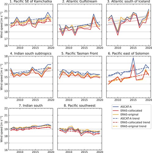
Table 2.1.2. Linear trends for ASCAT-A, collocated and original ERA5 [m s⁻¹ yr⁻¹] in the annual 99th percentiles over the period 2007–2020 for selected ocean regions.

A consistent negative 2020 anomaly and trend is found across the Tasman Front, the eastward branch of the East Australian Current (box 5). Gradients in the wind stress curl play a critical role in the separation point of the eastward flowing branch (Tilburg et al. Citation2001). Further analysis is needed to establish whether the reduction in extreme wind speeds is linked to more southward extension of the East Australian Current and recent marine heatwaves near Tasmania (Oliver et al. Citation2018).

Extreme wind speed trends are generally positive in the northern hemisphere storm tracks. Because of the large interannual variability, trends in the selected regions are not always statistically significant (boxes 1, 2 and 3). The extreme wind speed minimum south of Iceland in 2010 was also observed in the United Kingdom and associated with a strongly negative North Atlantic Oscillation index (Earl et al. Citation2013).

Compared to the northern hemisphere storm tracks, the interannual variability in the $P_{99 %}$ wind speeds in the southern hemisphere storm tracks is small (boxes 7 and 8). Contrasts between the ocean basins are large. Predominant and large positive trends are found in the southern Indian Ocean, while trends in the Pacific and Atlantic Ocean are generally small, both positive and negative and only locally significant. Negative trends prevail in the central-southern Pacific.

The bias between scatterometer and collocated ERA5 $P_{99 %}$ wind speed climatologies is positive at all latitudes ((c)), indicating that extreme winds are systematically lower in ERA5. Biases are typically 0.5 m s⁻¹, with maximum values around the equator and small biases in the Pacific Ocean around 5°S and the Indian Ocean near 20°N. The order of magnitude of the ERA5 biases is similar to the interannual variability in the scatterometer $P_{99 %}$ wind speeds.

The time series with annual $P_{99 %}$ wind speed percentiles for the selected regions corroborate that ERA5 extreme winds are consistently lower than ASCAT-A extremes (). Biases vary considerably between regions, ranging from 0.2 m s⁻¹ in the southern Indian and Pacific Oceans to 1 m s⁻¹ east of the Solomon Islands. Biases fluctuate little from year to year, but slightly increase over the 2007–2020 period for nearly all regions, resulting in lower trends with lower significance derived from ERA5 (). The biases are consistent with the lack of small-scale spatial variability, particularly meridional, in the ERA5 transient winds (Belmonte Rivas and Stoffelen Citation2019), since the spatially and temporally smooth ERA5 fields capture less extreme winds.

Spatiotemporal sampling effects estimated from the difference between original and collocated ERA5 $P_{99 %}$ winds fluctuate around 0 m s⁻¹ in the tropics, increasing to positive values around 0.3 m s⁻¹ for latitudes poleward of 30°N and S ((d)). Local differences reach ±1 m s⁻¹ in the mid-latitude storm tracks (not shown). The sampling noise magnitude does not relate to the number of observations, but rather to wind speed variability which is higher outside the (sub)tropics. Despite the small-scale noise associated with the sampling and the general underestimation of extreme wind speeds in the mid-latitudes, interannual anomalies and trends are robust on a regional scale (, ).

2.1.4. Conclusions and discussion

We have derived a global extreme wind climatology for the period 2007–2014 based on 99th percentile wind speeds from Metop-A ASCAT. An earlier global high wind speed climatology produced using part of the QuikSCAT SeaWinds scatterometer record (1999–2006), analysed the frequency of wind speeds exceeding 20 m s⁻¹ (Sampe and Xie Citation2007). While only a qualitative comparison is possible because of the different metrics, there is agreement on the windiest region (southernmost Greenland) and the general alignment of high wind areas with the storm tracks. Extreme wind speeds in the tropical regions are more distinct in our 99th percentile analysis.

Over the period 2007–2020, positive trends in annual extreme wind speeds were found to prevail on a global scale, although significant negative trends were observed in some regions. A trend analysis of extreme wind speeds (90th percentile) from altimeter observations over the period 1985–2018 revealed overall positive trends, with the largest trends (+0.05 m s⁻¹ yr⁻¹) in the southern hemisphere oceans below 30°S (Young and Ribal Citation2019). Scatterometer trends over the (different) period 1992–2018 were found to be smaller in the southern hemisphere and larger in the northern hemisphere. Although the different periods and percentiles used inhibit a direct comparison with our results, there is only weak correspondence with the longer-term study regarding the regions with the largest positive trends. This suggests that the long-term positive trends are subject to substantial variability on shorter timescales or dependent on contributing instruments, sampling and calibration.

The reference period used in this study represents a relatively short period in terms of climate variability. Observed changes reported may be linked to anthropogenic climate change, but could also result from natural variability. By combining multiple scatterometer records, the analysis could be extended backward to 1992, covering nearly 30 years of observations. However, zonal biases between available reprocessed scatterometer and ERA5 extreme winds records were found to be twice as large for Ku-band scatterometers (QuikSCAT SeaWinds and Oceansat-2 OSCAT) than for C-band scatterometers (Metop-A ASCAT, ERS-1 and ERS-2 SCAT). Improvements to be implemented in the next scatterometer reprocessing phase include intercalibration, a sea-surface temperature correction and revised quality control. This will likely reduce the biases between scatterometer instruments (Wang et al. Citation2019) and lead to a useful extension of this unique densely-sampled scatterometer record of extreme winds.

The spatiotemporal sampling of the ERA5 wind fields was found to introduce considerable noise at small spatial scales and underestimate the absolute extreme wind speeds outside the tropics. On regional scales, only minor differences in the interannual variability and trends were found between original and collocated ERA5 winds. While the ERA5 comparison results provide valuable insight into sampling effects, the scatterometer sampling noise characteristics may differ from the ERA5 results because small-scale variability is better resolved. The growing virtual scatterometer constellation may shed light on this, but only after successful intercalibration of the instruments.

This study only touched the surface of extreme wind speed aspects that can be analysed with a single scatterometer record. Future work may include seasonal variations and links to climate indices like the North Atlantic Oscillation (NAO) and the El Niño Southern Oscillation (ENSO). Regional variations and trends can be examined, as has been done for the Black Sea (Section 1.8 in this issue). By looking at higher percentiles, for instance the 99.9th percentile, tropical cyclone statistics can be derived. Last, by expanding the comparison of collocated and original (temporally homogeneous) ERA5 climatologies and trends, the gap between observational and model studies of extreme winds can be bridged.

Section 2.2. Overturning variations in the subpolar North Atlantic in an ocean reanalyses ensemble

Authors: Jonathan Baker, Richard Renshaw, Laura Jackson, Clotilde Dubois, Doroteaciro Iovino, Hao Zuo

Statement of main outcome: The magnitude and variability of the North Atlantic subpolar overturning circulation, and the associated heat and freshwater transports, measured across the OSNAP array from 2014 to 2018, are largely captured by an ocean reanalyses ensemble. Ocean reanalyses may therefore be a useful tool to understand the mechanisms that cause changes in the subpolar overturning of the North Atlantic, a region that is critically important for the maintenance of the overturning circulation. The ensemble-mean overturning is relatively stable over the 1993–2019 period, although there are significant shorter-term variations. Changes across both the east and west sections of the OSNAP array play an important role in its variability, despite a substantially stronger overturning strength across the east section.

Products used:

Table

2.2.1. Introduction

The Atlantic Meridional Overturning Circulation (AMOC) has an important role in the climate system by transporting heat northwards in the Atlantic (Srokosz et al. Citation2012). Since changes in the AMOC can have substantial impacts on ocean temperatures, and the wider climate, it is important to understand how the AMOC is changing. In particular, the AMOC is expected to have internal variability on many timescales (subseasonal-centennial) (Buckley and Marshall Citation2016), and increased greenhouse gases are expected to cause a long-term weakening trend (Collins et al. [Citation2019]). Although the RAPID array has measured the AMOC at 26.5°N since 2004, and has revealed shorter-term variability, it is not long enough to detect long-term trends (Srokosz et al. Citation2012). It also only measures the AMOC at one latitude, however AMOC variability can be different in the subpolar North Atlantic (Buckley and Marshall Citation2016). Some studies have suggested that the AMOC has already weakened over the last century (Rahmstorf Citation2015; Caesar et al. Citation2018; Thornalley et al. Citation2018), based on indirect methods relating the AMOC to observational proxies, however there are uncertainties in these methods (Moffa-Sánchez et al. Citation2019).

Since August 2014, the Overturning in the Subpolar North Atlantic Program (OSNAP) has continually observed the meridional transports of volume, heat and freshwater across the two sections of the OSNAP array (): OSNAP East to the east of Greenland and OSNAP West in the Labrador Sea (Li et al. Citation2017, Citation2021; Lozier et al. Citation2017). This has improved our understanding of the structure and variability of the overturning circulation in this region (Lozier et al. Citation2019; Zou et al. Citation2020), and the observations can be used to validate climate models (Menary et al. Citation2020). Only a 47-month period of observations is available, so longer-term variations must be inferred using ocean reanalyses or inverse models (e.g. Jackson et al. Citation2019; Fu et al. Citation2020).

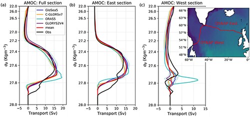
Figure 2.2.1. Vertical profile of the overturning transport in potential density space, averaged over the 47-month period of OSNAP observations, from August 2014 to June 2018, across (a) the full OSNAP section, (b) OSNAP East, and (c) OSNAP West. The reanalyses ensemble-mean (red, product ref 2.2.1) and spread (green shading) is plotted, along with each ensemble member, and the OSNAP observations (black, product ref. 2.2.2). The ensemble spread is calculated as two times the standard deviation across the ensemble members (excluding ORAS5). ORAS5 is excluded from the ensemble-mean and spread across all sections (see text). The map on the right shows the location of OSNAP East and OSNAP West (red lines).

We aim to extend these studies by comparing an ensemble of ocean reanalyses directly against OSNAP observations, to determine their ability to capture the observed transports. We also use the ensemble to infer longer-term variations in the meridional overturning circulation (MOC), across each section of the OSNAP array, prior to the availability of OSNAP observations. Ocean reanalyses may provide realistic three-dimensional estimates of past changes in the subpolar North Atlantic MOC and other ocean state variables, and thus could be a useful tool to infer the nature and cause of past MOC variability over various timescales. The reanalyses used in this study capture both the mean strength and variability of the overturning circulation across the RAPID array at 26°N with a high degree of accuracy (Jackson et al. Citation2016, Citation2018, Citation2019); thus, they may also accurately simulate changes across the OSNAP array.

2.2.2. Ocean reanalysis ensemble and methods

We use an ensemble of eddy-permitting (¼ degree horizontal resolution) global ocean reanalyses, product ref 2.2.1 (these are GloSea5 (MacLachlan et al. Citation2015), C-GLORSv7 (Storto et al. Citation2016), GLORYS2v4 (Lellouche et al. Citation2013) and ORAS5 (Zuo et al. Citation2019)), constrained by observations and ERA-Interim atmospheric forcings (Dee et al. Citation2011) over the period 1993–2019, with C-GLORSv7 extended to June 2020 and GloSea5 extended to December 2020. Each reanalysis uses the NEMO ocean model, but the sea-ice model and the data assimilation techniques differ. Each of the reanalyses assimilate satellite sea surface temperature (SST), sea level anomalies, sea-ice concentrations and in-situ temperature and salinity. Further details of each reanalysis product are in the aforementioned studies.

Ensemble-mean and spread over 1993–2019 and over the 47-month observational period are calculated. We exclude ORAS5 from the ensemble-mean and spread across all sections since the MOC across OSNAP West is an outlier from the ensemble and observations, with an anomalously large seasonal cycle ((c) and (a)). We note that the AMOC at 26.5°N in ORAP6, an updated version of ORAS5, is more realistic (Zuo et al. Citation2021), suggesting this may also be the case at OSNAP.

We calculate monthly-mean MOC across OSNAP East, OSNAP West and across the full OSNAP array in density coordinates, using methods described in Zou et al. Citation2020. We set volume transport to zero at the ocean floor (rather than the surface) in both observations and reanalyses to reduce errors at depth (Zou et al. Citation2020). Net transport through each section of the reanalyses is set equal to the corresponding net transport used in the observations, which is 1.6, −1.6 and 0 Sv across OSNAP East, OSNAP West and the full section respectively, where a positive transport represents a net northward flow. The net transports across these sections are similar among the reanalyses with a mean value over the observational period, prior to adjustment, of 1.6, −3.3 and −1.7 Sv respectively. We also calculate the heat and freshwater transports using the same methods as the observations (Lozier et al. Citation2019). Since there are net volume transports through sections, heat transports are defined as temperature transports and freshwater transports are referenced to the section mean salinity. We note that the precise definition of the transports does not impact the results significantly.

We use these monthly-mean observations and reanalyses data to calculate the overturning profiles and monthly-mean variability, with each figure based on this data. In we also use the Monte Carlo simulation observational mean and error estimates of Lozier et al. (Citation2017) and Li et al. (Citation2021) (further details therein). Since these are referenced to zero at the surface rather than at the ocean floor, we use the same method for the ensemble transports for direct comparison. This shifts the vertical profiles () and maximum overturning across OSNAP East and OSNAP West by 1.6 and −1.6 Sv respectively.

Table 2.2.1. Time-mean and uncertainty, and monthly-mean variability of the maximum MOC, and the meridional heat and freshwater transports (MHT and MFT) across the three OSNAP sections, for the ensemble-mean (product ref 2.2.1) and the OSNAP observations (product ref 2.2.2).

2.2.3. Results

The reanalyses capture the main structure of the observed overturning profile across each section (). AMOC across OSNAP East dominates that across OSNAP West. The maximum overturning strength across the full section is similar in the reanalyses to the observations, with a higher value than the observations across OSNAP East and a lower value across OSNAP West (). The southward flow below the maximum across OSNAP East and the full section is spread over a wider density range (i.e. the overturning strength reduces more gradually with depth) in the observations, and the reanalyses are missing transports in the densest layers. Nonetheless, the overall shape of the profiles and the densities of the maximum overturning in the reanalyses are similar to the observations across these sections.

In contrast, the overturning across OSNAP West is more diverse among the reanalyses and they diverge further from the observations ((c)). The local maxima and minima occur at different densities (it is worth noting that the vertical density scale in is non-linear) and therefore the profiles of the individual ensemble members rather than the ensemble-mean provide a more useful comparison to the observations. The reanalyses also capture the southward and northward flows observed below the maximum ((c)), although they do not capture the observed southward flow near the ocean floor. However, the reanalyses (except ORAS5) provide a reasonable estimate of the magnitude and structure of the overturning across OSNAP West.

We now focus on the variation of the monthly-mean maximum overturning ((a)). We note that the sum of the MOC across OSNAP East and OSNAP West is significantly larger than the MOC calculated across the full section because the peak overturning across OSNAP East and OSNAP West occur at different densities (). The time-mean overturning in the ensemble is stronger than observed across the full section and OSNAP East, but weaker across OSNAP West, although their uncertainty ranges overlap across each section (). The overturning variability in both observations and ensemble is greater across OSNAP East than OSNAP West ( and (b)), significant at p = 0.005 over both the whole reanalyses period and the observational period (using an F-test for equality of two variances). The ensemble-mean variability is significantly correlated with the observations across the full section (r = 0.66, p = 3.7 × 10⁻⁷), OSNAP East (r = 0.61, p = 4.3 × 10⁻⁶) and OSNAP West (r = 0.43, p = 2.9 × 10⁻³).

Figure 2.2.2. (a) Timeseries of the monthly-mean overturning transport, from August 2014 to June 2018 across (top) the full OSNAP section, (middle) OSNAP East, and (bottom) OSNAP West in the four reanalyses, the ensemble-mean (red, product ref. 2.2.1) and the OSNAP observations (black, product ref. 2.2.2). Labels and shading as in Figure 2.2.1. The horizontal grey dashed line in the lower plot divides the y-axis into two linear scales, with the y-axis compressed above the line. (b) Box plot of the monthly-mean MOC variability in the observations (green) and in the ensemble-mean (red) across each OSNAP section, over the same time period as in (a). The boxes represent the interquartile range (IQR) with the median line shown. The whiskers cover a range of values up to 1.5 times the IQR and the diamonds are outlying values beyond this range.

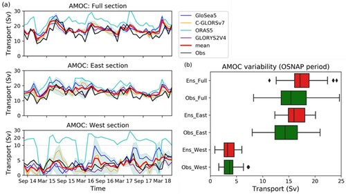
There is a significant seasonal cycle in the simulated overturning (see (a) and Jackson et al. Citation2019), in good agreement with the observations. The overturning is strongest in spring and weakest in winter ((a)). The average seasonal cycle of the ensemble-mean over the whole reanalyses period of 8.7 Sv is similar to the seasonal cycle over the 2014–2018 period (8.6 Sv), but this is smaller than that in the observations (12.6 Sv). In the observations, the seasonal range decreases gradually over the four-year observational period from 16.4 to 9.4 Sv, and tends to be greater than in the ensemble. This is due primarily to the monthly-mean overturning minima having a lower value in the observations.

Figure 2.2.3. Timeseries of (a) the monthly-mean and (b) the 12-month running mean, of the overturning transport from January 1993 to December 2020 across (top) the full OSNAP section, (middle) OSNAP East, and (bottom) OSNAP West. Labels, shading and product information are as in and . The horizontal grey dashed lines divide the y-axis into two linear scales, with the y-axis compressed above the line.

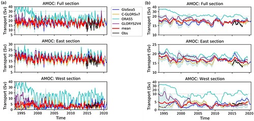
The 12-month running mean overturning is analysed over the whole period to infer longer-term variability ((b)). Although the ensemble appears to capture interannual variability across OSNAP East over the observational period, a longer observational timeseries is required to confidently analyse these longer timescale variations.

The reanalyses suggest the overturning has been relatively stable since 1993, with a similar ensemble-mean overturning across each section over the whole period to that during the observational period (). While the ensemble-mean (which excludes ORAS5) is relatively stable over 1993–2019, ORAS5 and GLORYS2 initially weaken, although the weakening in ORAS5 is likely due to an initialisation issue (Jackson et al. Citation2019). A decline in the AMOC at 45°N over 1993–2010 has been inferred in previous studies, with changes in the North Atlantic Oscillation a significant driver of this variability (e.g. Robson et al. Citation2012; Danabasoglu et al. Citation2016; Desbruyères et al. Citation2019). However, the MOC across OSNAP only declines over this period in two of our reanalyses, despite them all decreasing at 45°N (Jackson et al. Citation2019). The ensemble-mean MOC has a slight decline over 1993–2019 across all sections (), with the long-term trend equivalent to a weakening of ∼1.1, ∼1.9 and ∼1.5 Sv across the full section, OSNAP East and OSNAP West respectively (p = 0.007). However, the decline across the full section is only significant in GLORYS2 (excluding ORAS5), equivalent to a weakening over 1993–2019 of ∼3.8 Sv. Hence, there is uncertainty in the long-term trend from the ensemble at OSNAP.

There is a significant temporary weakening in the winters of 2008/09 and 2011/12, common to all reanalyses. Changes across both OSNAP East and OSNAP West contribute to these periods of weaker overturning, with the ensemble-mean across OSNAP West approaching zero in 2008/09. Variability over 1993–2019 is only slightly larger across OSNAP East than OSNAP West, despite the mean OSNAP East overturning being over four times larger ().

We also calculate the heat and freshwater transports (MHT and MFT) across the sections, although only the 21-months of observational data from August 2014 to April 2016 are currently available. Mean values are larger in the ensemble than in the observations, but the estimates of the ensemble-mean are within the observational uncertainty, except for the MFT across the full section (). Ensemble-mean MHT and MFT averaged over the observational period are approximately the same as over the whole reanalyses period.

2.2.4. Conclusions

An ensemble of global ocean reanalyses provides a realistic estimate of the magnitude and variability of the subpolar North Atlantic meridional overturning circulation (MOC) that has been measured across the OSNAP array between 2014 and 2018. The ensemble also provides a reasonable approximation of the meridional heat and freshwater transports across the OSNAP array.

The reanalyses slightly overestimate the magnitude and underestimate the variability of the overturning across the full section of the OSNAP array. The monthly-mean overturning is significantly correlated with the observations across all sections, although less of the variability is captured across OSNAP West. Nonetheless, the magnitude and structure of the overturning are reasonable approximations to the observations in all sections.

The overturning in the reanalyses ensemble has a small long-term decline, although this is not found in all the reanalyses, so is uncertain. The reanalyses suggest that there was an anomalously weak overturning in 2009/10 and 2011/12. Given the significance of the subpolar North Atlantic overturning on climate, further research is planned to understand the causes of these changes. Continual monitoring across the OSNAP array is critical to determine the ability of the ensemble to capture longer-term variations of the MOC.

To summarise, an ensemble of ocean reanalyses appears to be a useful tool to infer changes in the subpolar North Atlantic overturning. They enable variations prior to OSNAP to be estimated and the causes of these variations to be studied. Reanalyses and observations complement each other, to improve our understanding of the Atlantic meridional overturning circulation.

Section 2.3. Atmospheric and oceanic contributions to observed Nordic Seas and Arctic Ocean heat content variations 1993–2020

Authors: Michael Mayer, Takamasa Tsubouchi, Karina von Schuckmann, Vanessa Seitner, Susanna Winkelbauer, Leopold Haimberger

Statement of Main Outcome: The Arctic Mediterranean (Nordic Seas and Arctic Ocean together) plays an important role in the global climate system through its direct link with the Atlantic Meridional Overturning Circulation. Assessment using budget closure and validation with observation-based data demonstrates that the CMEMS ensemble reanalysis product along with atmospheric reanalysis and satellite data are useful products for exploring variability and trends in this region. The 1993–2020 rate of full-depth ocean heat content change in this region amounts to 0.8 (0.4, 1.0) Wm⁻² (bracketed values given the minimum-to-maximum range of estimates based on the employed datasets), with the Atlantic Water layer contributing ∼64%, the Overflow Water layer ∼31%, and Polar Waters ∼5% to the full-depth warming. Heat uptake by sea ice melt additionally added 0.2 (0.2, 0.3) Wm⁻² to the Arctic Mediterranean regional energy imbalance of this region. Ocean heat transport from the Atlantic into the Arctic Mediterranean is found to be a pacemaker of observed ocean heat content increase in the Arctic Mediterranean, and our results identify two drivers of the transports: wind-driven variability on interannual time scales, and Subpolar Gyre dynamics on decadal time scales. Since 2018 onwards however, ocean heat transport is decreasing, which opposes the strengthening over the past decades and warrants further studies.

Products used:

Table

2.3.1. Introduction

The North Atlantic Current transports warm and saline Atlantic waters northward. Some of this water flows to the Nordic Seas and Arctic Ocean (Arctic Mediterranean), where it is gradually cooled, mainly through air–sea fluxes, on its pathways (e.g. Hansen et al. Citation2008; Bosse et al. Citation2018). This cooling is strong enough to form dense waters that eventually contribute to overflow waters crossing the Greenland-Scotland ridge (Mauritzen Citation1996). Open ocean convection in the Nordic Seas is another mechanism to form dense water (Swift and Aagaard Citation1981). Since overflow waters crossing the Greenland-Scotland ridge feed back to the North Atlantic Meridional Overturning Circulation (AMOC), formation of dense water in the Nordic Seas and Arctic Ocean is an integral part of the global climate system (Hansen and Østerhus Citation2000; Buckley and Marshall Citation2016). In fact, ∼70% of the oceanic heat loss from the AMOC occurs north of the Greenland-Scotland ridge (Chafik and Rossby Citation2019). Through this strong link, variability and trends in the heat budget of the Arctic Mediterranean have not only regional impact, but global implications (e.g. Jackson et al. Citation2015). Quantification of the budget thus contributes to better understanding of important global climate processes of great relevance for society.

Numerous studies quantified different aspects of the heat budget of the Nordic Seas and the Arctic Ocean, using models (e.g. Muilwijk et al. Citation2018), reanalyses (e.g. Mayer et al. Citation2016; Asbjørnsen et al. Citation2019), or observations (e.g. Tsubouchi et al. Citation2018, Citation2021). Few attempts have been made to quantify the coupled ocean-ice-atmosphere energy budget of the region combining available observations and reanalyses to obtain a complete picture, informed and constrained by observations as much as possible. For example, Mayer et al. (Citation2019) used mass-conserving mooring-derived oceanic transports through the Arctic Gateways, ocean-ice and atmospheric reanalyses, and satellite data to provide an up-to-date estimate of the energy budget of the central Arctic with a remarkably small budget residual.

Here we follow a similar approach to explore the oceanic heat budget of the Arctic Mediterranean, the ocean bounded by the Greenland-Scotland Ridge (GSR), Davis Strait, and Bering Strait, with emphasis on interannual variability and its drivers. Newly available information from mooring-derived oceanic heat transports into the Arctic Mediterranean covering more than two decades (Tsubouchi et al. Citation2021) allow us to validate reanalysis-based transport estimates from the CMEMS GREP at these sections for the first time, which helps to build confidence in the use of this product for this type of application.

2.3.2. Data and methods

We study the heat budget of the Arctic Mediterranean over the 1993–2020 period. The vertically integrated heat budget of the ocean, including sea ice, is written as: (1) $F_{S} = \frac{\partial}{\partial t} OHC + \frac{\partial}{\partial t} ME + \nabla \cdot OHT + \nabla \cdot ILHT$ (1) F_S denotes the net surface energy flux (positive downward) at the air–sea/ice interface. It is computed as a residual from the atmospheric energy budget, as this has been shown to provide a more accurate estimate of F_S than model-based or purely satellite-based data (Von Schuckmann et al. Citation2016; Mayer et al. Citation2017; Trenberth and Fasullo Citation2017). Input data for evaluation of the atmospheric energy budget are net radiative fluxes at top-of-the-atmosphere from CERES-EBAF v4.1 (Loeb et al. Citation2018; product ref 2.3.1) and atmospheric transport and storage based on ERA5 (Hersbach et al. Citation2020; J. Mayer et al. Citation2021; product ref 2.3.2) and JRA55 (Kobayashi et al. Citation2015; Mayer et al. Citation2017; product ref 2.3.3).

OHC denotes the vertically integrated full-depth ocean heat content, ME sea ice melt energy, OHT vertically integrated ocean heat transport, and ILHT latent heat transport associated with sea ice. Following Mayer et al. (Citation2019), ME is computed as ME = L_f h_eff, where L_f is the latent heat of freezing (−0.33 × 10⁶Jkg⁻¹) and h_eff is effective sea ice thickness. Consequently, energy input to the sea ice, i.e. a positive ME tendency, leads to melting and vice versa. We compute OHC, ME, and OHT from the GREP ensemble (consisting of four eddy-permitting reanalyses at ¼° resolution) using monthly mean data (1993–2019; product ref 2.3.4), extended to 2020 using data from GREP member Ocean Reanalysis System 5 (ORAS5; Zuo et al. Citation2019, product ref. 2.3.4) due to the non-availability of the full GREP extension at time of writing. Sea ice transports and especially their contribution to budget anomalies are small at the boundaries of our study area, and hence only their contribution to the climatological mean ILHT is included based on the values provided by Tsubouchi et al. (Citation2021).

Following Gauss’ theorem, the ocean heat divergence integrated over our study area can alternatively be computed as the sum of the oceanic boundary fluxes into the region. This allows us to additionally use mooring-based observations of OHT from GSR, Davis Strait, and Bering Strait, available for 1993–2016 (Tsubouchi et al. Citation2021; product ref 2.3.5) for computation of the divergence term.

To gain a better process understanding, we also explore contributions from Polar waters (PW) and Atlantic waters (AW) to full-depth OHC. For the water mass definition, we follow Rudels et al. (Citation2008) by defining PW by $σ_{P W}$ < 27.70 kg m⁻³, where $σ$ is defined as sea water density minus 1000. Additionally, we define PW to be cooler than 4°C. The threshold for the lower boundary of AW is determined by checking water density in the GSR east of Iceland at the depth where water temperature is 4°C. This yields an AW definition of $27.7 < σ_{A W}$ < 30.00 kg m⁻³, where the latter is similar to the upper boundary of Deep Water provided by Rudels et al. (Citation2008). The water mass below AW is termed Overflow Water (OW).

For additional diagnostics over the study period, we use reprocessed sea level anomaly (SLA) data from AVISO (product ref 2.3.6; available 1993–2019) and Arctic Oscillation (AO), North Atlantic Oscillation (NAO), and Pacific North-American Pattern indices obtained from NOAA (product ref 2.3.7). As the major objective of this study is to address changes at interannual and longer time scales, the anomaly time series have been smoothed using a 12-monthly window, except for the heat accumulation plot (a). Values are generally given in Wm⁻² w.r.t area of the Arctic Mediterranean of 13.08 × 10¹²m² (i.e. the conversion factor to TW is 13.08). Statistical significance of Pearson’s correlation coefficients (r) takes auto-correlation of the time series into account, following Oort and Yienger (Citation1996). Uncertainties are provided as minimum-to-maximum range of different estimates (in brackets) or as total error standard deviation (±).

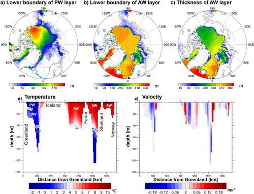
Figure 2.3.1. Climatologies of lower boundaries of (a) PW and (b) AW layers as well as (c) layer thickness of the AW layer. Light blue line in (a) indicates the boundaries of the Arctic Mediterranean. GREP (product ref 2.3.4) ensemble mean climatological (d) temperature along with water masses and their vertical (σ-based) and horizontal (temperature-based) boundaries (see section 2.3.2 for definitions) and (e) current cross sections across the Greenland-Scotland-Ridge.

2.3.3. Results

2.3.3.1. Arctic water masses in the reanalysis products

presents the 1993–2020 mean lower boundary of (a) Polar Water (PW) and (b) Atlantic Water (AW) based on the GREP ensemble mean (product ref. 2.3.4). The GREP ensemble mean climatological and area-average PW layer thickness is 70.0 (64.2, 75.9) m for the Arctic Mediterranean. Most of the layer’s volume is located under sea ice (∼97.5% of the PW volume are located in regions with >30% sea ice concentration), with maximum thickness of up to 200 m in the Amerasian Basin. The AW layer is located under the PW (where it is present), but outcrops to the surface primarily in the Norwegian Sea, Barents Sea, and the western Nansen Basin, north and northeast of Svalbard (Bosse et al. Citation2018; Skagseth et al. Citation2020; white areas in (a)). The AW layer has an area-average thickness of 227.7 (223.6, 230.1) m ((b,c)) and attains a thickness of more than 400 m in the Nordic Seas. (d) shows a longitude-depth cross-section of climatological temperatures along the GSR based on GREP data and also indicates the locations of the three water masses. The plot shows the large Atlantic Water body, extending eastward from the Eastern Denmark Strait to the coast of Norway and down to depths of ∼400 m, in good agreement with observations (e.g. Hansen et al. Citation2008). (e) shows a cross-section of climatological currents across GSR, which show the four main branches of Atlantic Water inflow in the North Icelandic Irminger Current (Jónsson and Valdimarsson Citation2012), the Iceland–Faroe (Hansen et al. Citation2015) and the Faroe–Shetland Channel branches (Berx et al. Citation2013), and the European Shelf Branch (Østerhus et al. Citation2019), in good qualitative agreement with observations.

2.3.3.2. Budget closure

Before exploring trends and variability of the heat budget of the Arctic Mediterranean, we first address the closure of the regional heat budget of the Arctic Mediterranean to assess the consistency of the used data products. Ideally, the lateral and vertical energy fluxes into the study area should add to balance the sum of oceanic storage rates OHCT + MET (appended ‘T’ indicates time derivative of OHC and ME), which is on the order of 1 Wm⁻² (see below, and Mayer et al. Citation2019; compare Equation (1)). There is good agreement between the 1993–2016 long-term mean OHT estimated from moorings (23.4 ± 2 Wm⁻², with uncertainties based on values provided by Tsubouchi et al. Citation2021) and from the GREP ensemble (20.1 (18.5, 21.6) Wm⁻²; values in brackets provide the range of values from the 4 reanalyses in the GREP). Note that the provided uncertainty for the GREP-based OHT is similar to a total error estimate of ±1.7 Wm⁻² derived from adding spread of the four reanalysis-based long-term means, i.e. systematic error, and the standard error of annual averages of the GREP ensemble mean, i.e. random error, in quadrature. The 1993–2020 average F_S in our study area is −27.6 and −29.4 Wm⁻², when using atmospheric transports from ERA5 or JRA55, respectively. The smallest budget residual is obtained when we combine observation-based OHT and ERA5-based F_S, with the energetic contribution of sea ice transports of ∼0.4 Wm⁻² (Tsubouchi et al. Citation2021) added, which yields a long-term flux convergence or heat input (=F_S+OHT + ILHT) of −3.8 Wm⁻². This value indicates an imbalance between diagnosed oceanic heat input and ocean heat storage (∼1 Wm⁻²) on the order of 5 Wm⁻². Note that the diagnosed budget imbalance attains up to ∼10 Wm⁻² for less favourable combinations of data sets. This systematic imbalance suggests that either diagnosed surface heat loss is too strong or OHT is too weak (or both). The former could arise from a negative bias in poleward atmospheric energy transports used for estimation of F_S, and for which in-situ based measurements for validation do not exist with the required spatial sampling. CERES-EBAF data going into F_S as well is assumed to have only a small bias (Loeb et al. Citation2018; Mayer et al. Citation2019). Underestimation of OHT may arise from spatial undersampling in the case of observations, while the GREP-based OHT additionally suffers from underestimation of eddy transports due to the use of monthly mean data.

In terms of variability, we find high correlation between anomalies of ocean heat flux convergence and the rate of total ocean heat storage (OHCT + MET), with r ∼ 0.74 (significance level p < 10⁻⁸) for the full 1993–2020 period and r ∼ 0.9 (p < 10⁻⁸) for the observation-rich 2005–2020 period (similar for different products). Temporal standard deviation of ocean heat flux convergence is ∼2.2 Wm⁻² (2.5 Wm⁻²) and that of OHCT + MET is ∼2.4 Wm⁻² (2.5 Wm⁻²) for the 1993–2020 (2005–2020) period, while that of the budget residual is ∼1.5 Wm⁻² (1.1 Wm⁻²). These results suggest that our estimates of the different physical terms exhibit consistent temporal variability, with a reasonably high signal-to-noise ratio especially during the observation-rich 2005–2020 period.

2.3.3.3. Time evolution of the Arctic Mediterranean heat budget

(a) presents oceanic heat accumulation averaged over the Arctic Mediterranean for the period 1993–2020. Full-depth ocean heat content increased, with an ensemble mean trend of 0.8 (0.4, 1.0) Wm⁻². The ocean warmed in this area at varying pace, with periods of rapid warming during 2002–2008, 2011–2012, and 2015–2017. (a) shows that the Atlantic Water (AW) layer contributes roughly 64% of the full-depth OHC increase, with an ensemble mean trend of 0.5 (0.3,0.7) Wm⁻². Moreover, the AW layer OHC shows very similar periods of rapid and slow warming compared to the full-depth OHC estimate, rendering it as a pacemaker of the full-depth OHC. Polar Water (PW) OHC increased more moderately (ensemble mean trend is 0.0 (0, 0.3) Wm⁻², or 0.04 (0.01, 0.32) Wm⁻² when allowing for two decimals), mainly due to its smaller volume of which the majority is covered by sea ice (see discussion above). The trend in melt energy over the entire study period amounts to 0.2 (0.2, 0.3) Wm⁻² ((a)).

Figure 2.3.2. (a) Heat accumulation of the Arctic Mediterranean, represented as full-depth ocean heat content (OHC) (along with PW and AW contributions) and heat used for sea ice melt (ME); (b) time derivative (indicated by appended ‘T’) of quantities shown in (a); (c) anomalous ocean heat transport into Arctic Mediterranean from the GREP (product ref 2.3.4; shading represents ensemble spread) ensemble mean and observations (product ref 2.3.5; shading represents uncertainty based on 26 TW provided by Tsubouchi et al. (Citation2021), reduced by the factor $1 / \sqrt{2}$ as discussed in the text); (d) inferred net surface energy flux (F_S), combining CERES-EBAF (product ref 2.3.1) net TOA fluxes and atmospheric budgets from ERA5 (product ref 2.3.2) and JRA55 (product ref 2.3.3), respectively, averaged over the Arctic Mediterranean. All quantities are presented with the annual cycle removed, and a 12-point running mean was applied to time series in (b) to (d).

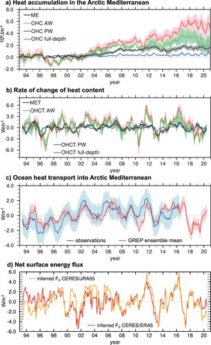
PW OHC and energy used for sea ice melt exhibit a coherent evolution, particularly in 2015–2017, confirming the tight coupling between the two terms: anomalously strong surface energy input leads to a reduction of sea ice cover. Consequently, heat absorption by the newly exposed waters is enhanced. In addition, PW can also be warmed by enhanced upward mixing of AW heat, which then in turn contributes to anomalous sea ice melt (Polyakov et al. Citation2017).

While (a) provides a time-aggregated perspective on heat accumulation in the Arctic Mediterranean, (b) converts the quantities to rates of change, which makes them comparable to ocean heat transport and surface flux anomalies, and additionally emphasises interannual variations. OHCT of the AW layer is highly correlated with full-depth OHCT (r = 0.94, p < 10⁻²⁴), confirming the dominant role of AW full-depth OHC variability also on interannual time scales. Correlations of PW and OW with full-depth OHCT are lower (0.29 and 0.38, respectively), but nevertheless significant on the 95% confidence level.

Contributions to the heat content rate of change from ocean heat transport (OHT) are shown in (c). The OHT estimate from the GREP is in good agreement with the observation-based estimate as reflected by reasonably high correlation (r = 0.68) and mostly overlapping uncertainty intervals. Uncertainties of anomalies are estimated from the ensemble spread (defined as the standard deviation across the four members) in the case of the GREP. The uncertainty of the observation-based OHT is based on the total error of 26TW given by Tsubouchi et al. (Citation2021), but reduced by a factor of $1 / \sqrt{2}$ assuming that roughly half of the total error is a bias and hence irrelevant for anomalies. This assumption is deemed justified given the discussion of errors in Berx et al. (Citation2013), Hansen et al. (Citation2015), and Jónsson and Valdimarsson (Citation2012). The good agreement of our OHT estimates provides confidence in the signals displayed by the reanalysis product. Importantly, OHT from GREP shows similarly increased OHT after ∼2002 as found in the observations (Tsubouchi et al. Citation2021).

Interannual variations of OHT exhibit considerable co-variability with OHCT. When considering correlation of OHT with OHC tendencies of different water masses, the correlation is strongest with the AW OHCT (r = 0.62), similar to the correlation with the full-depth OHCT (r = 0.62, p < 10⁻⁴). This is consistent with AW inflow being an important driver of OHT across the GSR (Tsubouchi et al. Citation2021), and suggests that variations in ocean heat transports play an important role for modulations of AW OHC and hence also full-depth OHC of the Arctic Mediterranean. Correlations of PW OHCT and OW OHCT with OHT are lower, with r = 0.29 and r = 0.06, the latter being statistically insignificant.

(d) presents net surface energy flux anomalies (F_S) averaged over the Arctic Mediterranean. F_S is highly correlated with AW (r = 0.60) and PW OHCT (r = 0.39) (r of AW plus PW OHCT with F_S is ∼0.65), as these water masses are in touch with the surface (compare ). In contrast, correlation of F_S with OW OHCT is close to 0. (b) also shows two prominent peaks in OHC tendency in 2011 and 2016. Contributions to the heat content rate of change from ocean heat transport ((c)) and net surface energy flux ((d)) show that these two peaks are associated with coinciding peaks in OHT and F_S. Analysis of anomaly maps along with mean sea level pressure and near-surface winds (not shown) reveal that the strongest contribution to both the positive 2011 and 2016 F_S anomalies came from the Nordic and Barents Seas and was associated with southerly wind anomalies over this region. However, the associated mean sea level pressure pattern projected on the AO pattern only in 2011 but not in 2016 (compare (d) below). In general, the AO and NAO indices and F_S averaged over the Arctic Mediterranean do not correlate at the interannual time scales considered here. Similarly weak correlation is found for area-averaged F_S with the Pacific North-American Pattern index (not shown). We nevertheless stress that regional correlations between F_S and atmospheric circulation indices are higher, e.g. in the Nordic Seas and Barents Seas for the NAO and AO, but strong spatial compensation of regional anomalies occurs when averaging across the Arctic Mediterranean. The weak correlation of area-averaged F_S with atmospheric circulation indices also emphasises the important role of additional factors modulating F_S, such as sea ice concentration anomalies, which can greatly amplify or damp flux anomalies arising from atmospheric circulation anomalies through modification of the open water area available for strong turbulent air–sea fluxes (Shu et al. Citation2021) and ice-albedo feedback (Curry et al. Citation1995). Another important factor is the (negative) surface flux feedback to ocean heat anomalies in the Nordic Seas (i.e. positive OHC anomalies go with enhanced surface heat loss and vice versa, see, e.g. Muilwijk et al. Citation2018 or Årthun and Eldevik Citation2016), which appears to be more dominant on interannual timescales than atmospheric forcing.

Figure 2.3.3. Contemporaneous correlation (shading) and regression (contours) of Sea Level Anomaly from AVISO (product ref 2.3.6) with (a) OHT from GREP (product ref 2.3.4), (b) OHT from observations (product ref. 2.3.5), and (c) the Arctic Oscillation (AO) Index (product ref 2.3.7); Stippling indicates significant correlations at the 95% confidence level; (d) standardised anomaly time series of OHT from GREP and observations, AO Index, and the SLA-based proxy of OHT (see Equation (2)).

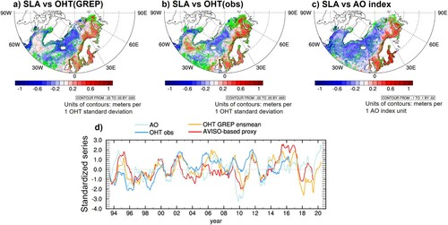
2.3.3.4. Drivers of ocean heat transports

We now further explore variability of net OHT into the Arctic. (a,b) show correlation maps of OHT and SLA. Both maps show that positive net OHT anomalies are associated with anomalously high sea levels in the eastern and low sea levels in the western part of the Nordic Seas (vice versa for negative OHT anomalies). Since net OHT into the Arctic Mediterranean is very strongly correlated with OHT across the GSR (r = 0.98 for GREP and r = 0.99 for observations), we interpret results from (a,b) mainly in terms of transports across the GSR. The correlation patterns in (a,b) suggest that OHT across the GSR is enhanced with a stronger west–east SLA gradient. This is consistent with Richter et al. (Citation2012) finding stronger AW inflow over the Iceland Faroe Ridge associated with SLA patterns in the Nordic Seas similar to those shown in (a,b). Performing correlations between OHT and bottom-pressure-equivalent SLA from ORAS5 gives similar patterns (not shown). This indicates that the SLA patterns are mainly related to mass redistribution in the Nordic Seas and associated changes in geostrophic currents.

Another salient feature of the correlations between OHT and SLA is the local maximum in the Northwest Atlantic, resembling the shape of the North Atlantic Subpolar Gyre (SPG). This feature is more prominent in the correlation between SLA and OHT from observations, but clearly visible also in the correlations with the reanalysis results. Positive OHT anomalies are associated with above-average sea level in the SPG region, which is indicative of a weakened SPG. A correlation map of net OHT with the barotropic stream function confirms this result (not shown).

Correlation between net OHT and the Arctic Oscillation (AO) index are 0.42 (p < 0.01) for the GREP (1993–2020) and 0.33 (p < 0.05) for observations (1993–2016), much higher than the (insignificant) correlation with NAO. Hence, (c) shows contemporaneous (lag 0) correlations of SLA and the AO Index. Patterns in the Nordic Seas are similar to those found in (a,b), which suggests that SLA variability associated with OHT variability is wind-driven, strongly linked to the AO. In contrast, the local maximum in the SPG region is not visible (even significantly negative values when correlating with NAO, not shown) in (c), suggesting that the wind forcing associated with the AO (or NAO) leads to SLA (and ocean circulation) responses in the SPG and Nordic Seas regions with competing effects on net OHT. We conclude that SLA patterns associated with net OHT anomalies (i.e. patterns shown in (a,b)) arise from a favourable combination of wind forcing in the Nordic Seas and longer-term variability of the SPG. Altogether, these results indicate that there is (i) strong wind-driven variability of OHT on interannual timescales (largely in agreement with earlier studies, e.g. Bringedal et al. [Citation2018]) and (ii), given the relatively long time scale of SPG variability (≥5 yrs, see Williams et al. Citation2015), an additional modulation of OHT by the SPG on multi-year timescales.

The strong relationship between the SLA gradient along the GSR and OHT provides motivation to define a SLA-based proxy (2) $OH T_{proxy} =< (SL A_{East} - SL A_{West}) >,$ (2) where the eastern box is bounded by 2°W–0°E, 58–60°N, and the western box is bounded by 20°W–15°W, 63–67°N, and <> denotes standardised anomalies. The result is shown in (d), along with standardised OHT from GREP and observations. Correlations between OHT_proxy and the explicit OHT estimates from GREP are 0.64 (1993–2019; p < 10⁻⁴) and for observations 0.40 (1993–2016; p < 0.1), respectively. This is higher than the direct correlations of OHT with AO (given above; series shown in (d) as well). This result demonstrates that the SLA gradient along GSR contains more relevant information about OHT than the AO index alone. We also note that we performed similar diagnostics using the NAO index, but correlations were generally lower.

The good agreement between GREP-based and mooring-derived OHT anomalies during 1993–2016 provides confidence in the diagnosed OHT variations in more recent years, when no observations are available. (b) shows a strong reduction of OHT 2018–19, with the lowest OHT values of the study period. The SLA-based proxy qualitatively confirms this reduction. Further diagnostics suggest that reduced AW inflow through the Faroe–Shetland Channel was a main contributor to this anomaly (not shown). OHT anomalies show a recovery towards neutral values in 2020, but the 2020 values are based only on one reanalysis product (see Section 2.3.2). Hence, whether the 2018–19 anomaly is merely an intermittent signal or marks the end of the period of increased OHT (ongoing since ∼2002) requires further investigations.

2.3.4. Discussion and conclusions

This contribution uses reanalyses and observation-based products to depict the mean state, variability, and trends of the Arctic Mediterranean heat budget. We evaluated the representation of Atlantic (AW), Polar (PW), and Overflow (OW) water masses in the GREP reanalysis product, which is in good qualitative agreement with observation-based work (Rudels et al. Citation2008). We then decomposed the full-depth OHC of the Arctic Mediterranean into contributions from the different water masses. The 1993–2020 full-depth OHC trend in the study area is 0.8 (0.4, 1.0) Wm⁻², which is in good agreement with results of Mayer et al. (Citation2021), who quantified OHC trends north of 60°N. AW contributes roughly 64% to the full-depth warming, and it plays an even more important role on interannual time scales, where it explains more than 90% of the variance of full-depth OHC tendencies. This is because the AW layer is the main water mass directly exposed to variations in air–sea fluxes (mainly in the Nordic Seas, compare (a,b); also note that PW is mostly under sea ice) and current and temperature variations of the inflow across the GSR directly impact OHC of this layer.

Assessment of closure of the diagnosed heat budget of the Arctic Mediterranean reveals long-term mean imbalances ranging from 5 to 10 Wm⁻², depending on the combination of data sets. The smallest imbalances are obtained when combining satellite-based radiation, atmospheric energy transports from ERA5, and mooring-derived OHT. Note that these three products are fully independent of each other. The OHT diagnosed from the GREP is biased low by ∼14%, which may be related to the use of monthly mean fields, leading to neglect of eddy heat transport. Overall, the budget residuals are larger than those reported by Mayer et al. (Citation2019) for the central Arctic. More work is needed to identify the main contributor (inferred air–sea fluxes over the Nordic Seas or OHT across the GSR or both) to the larger residuals.

Periods of rapid (moderate) OHC increase coincide with periods of anomalously strong (weak) ocean heat transport into the Arctic Mediterranean. Correlation analysis reveals two important drivers of OHT. First, there is strong wind-driven OHT variability (via modulation of zonal SLA gradients in the Nordic Seas) on interannual time scales. This is consistent with Richter et al. (Citation2012) and Bringedal et al. (Citation2018), although the latter emphasise the role of wind forcing on the seasonal timescale (which we did not study here) and additionally find increasing importance of the Nordic Seas SLA itself (rather than the zonal gradient) in forcing the Overturning Circulation in the Nordic Seas on interannual timescales. It is also important to note that Muilwijk et al. (Citation2018), based on a forced model run without data assimilation, found similar OHT-wind relationships as presented here but with pronounced decadal variations in the strength of the relationships, which we cannot assess given the length of the GREP record. Second, we found a negative correlation of OHT with the Subpolar Gyre (SPG), which modulates the transports on decadal timescales. This is consistent with earlier studies (e.g. Hátún et al. Citation2005; Asbjørnsen et al. Citation2021) who argue that a weak SPG extends less to the east, which allows more warm subtropical Atlantic waters to arrive at the GSR, leading to a temperature-driven enhancement of OHT across the GSR.

The good agreement of the GREP-based results with observation-based OHT estimates in terms of mean and variability builds confidence in the reanalysis product for usage as a complement to observations in order to get a spatially and temporally more complete picture of the Arctic Mediterranean.

Funding

This contribution was financially supported by Austrian Science Fund project P33177, CMEMS 114-R&D-GLORAN-CMEMS LOT 8, and CMEMS 21003-COP-GLORAN Lot 7.

Section 2.4. Changes in the Antarctic marginal ice zone

Authors: Doroteaciro Iovino, Julia Selivanova, Thomas Lavergne, Andrea Cipollone, Simona Masina, Gilles Garric

Statement of main outcome: The Southern Ocean plays a crucial role in the regulation of the global climate system, and the variation of its ice-covered area modifies the exchange of heat, mass and momentum between ocean and atmosphere. Therefore, knowledge of ice extent and its variability is necessary for an adequate simulation of those fluxes and thus for climate modelling. This section uses an ensemble of global eddy-permitting reanalyses (GREP) together with a Climate Data Record of Passive Microwave Sea Ice Concentration to investigate changes of Antarctic extent of the Marginal Ice Zone (MIZ) over the period 1993–2020. We assess the accuracy of GREP in discriminating the MIZ from the consolidated pack ice, and in reproducing their evolution in space/time. Although the ensemble reanalysis product tends to slightly overestimate summer MIZ, results show that it properly represents the variability of minima and maxima in MIZ extent as well as its interannual variability during the growing and melting seasons, particularly over the winter season. On average, the MIZ advance needs about 10 months to progress from near the coast in February to its most equatorward maximum and about only 2 months to return to a minimum. The MIZ extent did not experience a significant average trend over the study period, but the results further highlight substantial regional trends, particularly for regions covered by marginal ice.

Products used:

Table

2.4.1. Introduction

The Antarctic sea ice plays a crucial role in the regulation of the global climate system, and the variation of the ice-covered area modifies the exchange of heat, mass and momentum between ocean and atmosphere. Therefore, knowledge of ice extent and its variability is necessary for an adequate simulation of those fluxes and thus for climate modelling.

Unlike the Arctic, where sea ice extent (SIE) is decreasing in the entire region in all seasons, Antarctic trends are less noticeable and less clear (Simmonds Citation2015; Maksym Citation2019). While the Southern Ocean around Antarctica has been warming at an alarming rate contributing to ice sheet melt and consequently to sea-level rise, Antarctic SIE has remained stable (Parkinson Citation2019): the long-term SIE trend, on hemispheric scale, is nearly flat, for the winter maximum, summer minimum and annual average, although some regions experienced declines. Since the late 1970s, satellite record of total annual-mean extent shows a slight overall positive trend (Eayrs et al. Citation2021), which masks significantly larger opposing regional trends. The total Antarctic SIE has increased at a rate of approximately 1.5% per decade for the 1979–2015 period (e.g. Comiso et al. Citation2017), with a record high (of 12.8 × 10⁶ km²) reached in 2014 (Parkinson Citation2019). Many extreme events have been observed in recent years, with record-high winter maxima (occurring in September) in 2012–2015, followed by unprecedented decline with record low summer minimum extents (occurring in February/March) in 2016–2018 – the lowest value of 10.7 × 10⁶ km² reached in 2017 (Parkinson Citation2019). Despite this marked decrease since late 2016, the overall long-term trend (1979–2021) remains positive, but it is of lower magnitude than the 1979–2016 trend, and is no longer significantly different from zero. Although several explanations have been proposed for Antarctic sea ice changes, as changes in upper ocean stratification and in the atmospheric dynamics and winds (e.g. Hobbs et al. Citation2016), how these changes link with polar and global climate change is still puzzling.

While the reasons for variability in total extent remain not completely understood, it is likely that these changes are not just affecting the total Antarctic SIE but also the distribution and variability of pack ice, marginal ice zone (MIZ) and sparse ice, in other ways (Stroeve et al. Citation2016). Knowledge of the spatial pattern of these different ice classes may help to elucidate the mechanisms contributing towards the expansion of Antarctic ice in some regions and contraction in others (Maksym et al. Citation2012). In spite of the vast winter cover, sea ice around Antarctica forms a very thin layer on the ocean, with less than 1 m thickness on average, and more compact ice remains all year around only in a few coastal regions (Worby et al. Citation2008; Holland et al. Citation2014).

Several criteria for characterising the MIZ have emerged over the past decades, but finding a coherent definition is still a challenge. The MIZ was originally described as the region where polar air, ice and water masses interact with the ocean temperature and subpolar climate system (Wadhams et al. Citation1981). Now, it is commonly defined as the portion of the ice-covered ocean where surface gravity waves significantly impact the dynamics of sea ice (e.g. Wadhams Citation2000; Dumont et al. Citation2011), often characterised by highly variable ice conditions. Given the unknowns in wave-ice interaction and the large uncertainties in both observed and forecasted waves within sea ice, the MIZ can be operationally defined through sea ice concentration thresholds, as the transition zone between open water and consolidated pack ice, where the total area of ocean is covered by 15–80% sea ice (e.g. Paul et al. Citation2021; Vichi Citation2021).

The MIZ is fundamental for climate dynamics and polar ecosystems, as a region of intense atmosphere-sea ice interactions that forms a physical buffer for the consolidated pack ice zone from the effects of open ocean dynamics (e.g. Squire Citation2007). The MIZ supports relevant processes, such as air–sea gas exchange, and carbon exchange at the air–sea interface, marine primary production and delivery of nutrients to the euphotic zone (Barber et al. Citation2015). Monitoring changes of the MIZ environment can help us understand the associated changes in the climate system. Due to the thin and small broken ice floes, the MIZ region is highly dynamic and responsive to external forcing, and its response to climate variability differs from the inner pack ice (Stroeve et al. Citation2016). An accurate assessment of variability of dynamics in the MIZ is still missing, as well as a deep insight into how surface ocean/waves and atmospheric fields correlate with ice conditions, such as ice thickness, strength, and viscosity (Meylan et al. Citation2014; Sutherland and Balmforth Citation2019).

There are few in-situ data available on the Antarctic MIZ properties and still significant differences in estimates from satellite data sets depending on the algorithm employed (Stroeve et al. Citation2016). Numerous methods have been developed to estimate SIC from passive microwave instruments (including SMMR, SSMI, SSMIS, AMSR-E and AMSR-2) flying on various satellite platforms. The algorithms applied to the microwave brightness temperatures employ different channel combinations, with different corrections for weather, satellite drift, and other factors (Ivanova et al. Citation2015; Tonboe et al. Citation2016). When using estimates of sea ice properties, we should be conscious of the differences among algorithms and their attributes (Wright and Polashenski Citation2018), and the methods for combining different source data into long-term records (Stroeve et al. Citation2016).

Therefore, ocean/sea ice reanalysis data are essential in increasing our ability to comprehend total and marginal ice variability and to monitor their current state and predict their future changes. In this contribution, we aim to investigate how the Antarctic extent of MIZ is actually changing, using sea ice concentration from an ensemble of global eddy-permitting reanalyses (GREP), and to determine how realistically this product can capture the time/space variability of the Antarctic ice in the marginal ice zone over the period 1993-onward.

2.4.2. Methodology

The Global Reanalysis Ensemble Product (GREP version 2, product ref 2.4.1) is based on four global ocean reanalyses ORAs (GLORYS2v4, Lellouche et al. Citation2013; GloSea5, MacLachlan et al. Citation2015; C-GLORSv7, Storto et al. Citation2016; ORAS5, Zuo et al. Citation2019), constrained by satellite and in-situ observations and driven by ERA-Interim atmospheric reanalysis (Dee et al. Citation2011).

Each ORA uses the ocean component of the state-of-the-art NEMO model at eddy-permitting resolution (1/4° horizontal resolution), but the data assimilation techniques and the sea ice models differ (three ORAs employ the LIM2 sea ice model, one CICE4.1 that includes more complex physics compared to LIM2). Each of the reanalyses assimilates satellite sea surface temperature (SST), sea level anomalies, sea-ice concentrations and in-situ temperature and salinity. Details of each reanalysis product are in the above-mentioned studies. Single products as well as the multi-model ensemble are available from the beginning of the satellite altimetric era, January 1993 up to December 2020 (only Near Real Time altimetry data are ingested by the assimilation systems for the last six months).

The total ice is here split into three different zones. Due to the lack of wave estimations in the region and the availability of SIC observed-data, we use the concentration-based definitions for the GREP (product ref 2.4.1) output as well as the observational dataset (product ref 2.4.2), on their original grids. The consolidated pack ice is then defined by a SIC from 0.80 to 1. The MIZ is identified by SIC in the 0.15–0.80 range. Sparse sea ice covers regions with SIC lower than 0.15; it is worth mentioning that such low SIC can appear inside the pack ice region as well, in areas of potential polynyas.

To map Antarctic MIZ from satellite data record, we use the NOAA/NSIDC Climate Data Record (hereafter CDR, Meier et al. Citation2017, product ref. 2.4.2) that provides a combination of SIC estimates from two well-established algorithms (NASA Team and Bootstrap), reducing the overall low bias in a fully automated procedure (Peng et al. Citation2013). We use the merged product as each algorithm has different pros and cons. Stroeve et al. (Citation2016) analysed the Antarctic MIZ from the NASA Team (NT) and Bootstrap (BT) data, and showed that (1) the BT algorithm halves the MIZ and doubles the consolidated pack ice area compared to the NT algorithm; (2) trends are also different with the BT indicating no statistically significant trends in the MIZ, and NT statistically significant positive MIZ trends in spring. The root mean square errors of SIC between the ensemble mean and NOAA/NSIDC CDR (product ref 2.4.2) is presented for September and February climatology over the period 1993–2019 (). A RMSE up to 10% is visible in winter time over the Antarctic Circumpolar Current location, while summer SIC differs from satellite estimates mainly along the coastline of Eastern Antarctica where polynyas and ice sheets are present. CMEMS distributes global reprocessed SIC data from EUMETSAT OSISAF CDR and Interim CDR. This data set is ingested by some of the data assimilation systems employed in the ORAs constituting GREP (product ref 2.4.1), and hence not used for comparison in this study.

Figure 2.4.1. GREP SIC root mean square error for September (left), and February (right) averaged over 1993–2020 as derived from NOAA/NSIDC CDR (product ref. 2.4.2).

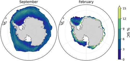
For all products, we analyse monthly means of SIC (the fractional coverage of an ocean grid-cell area covered with sea ice) to compute SIE as the total ocean area of all grid-cells with SIC exceeding 0.15. Thus, the MIZ extent represents the total area of ocean where SIC is comprised between 0.15 and 0.80. SIE is widely used as polar climate indicator minimising the effects of uncertainties in passive microwave estimates (e.g. Meier and Stewart Citation2019) compared to sea ice fraction and area. Our results are presented as hemispheric average, but we also show that sea ice variability and trends can regionally differ from the circumpolar ones.

2.4.3. Results

The climatological mean seasonal cycle of Antarctic MIZ does not follow total extent seasonality (). While both reach minima in February, the MIZ extent peaks after the annual total (and pack) sea-ice maximum, generally occurring in September. On average, the MIZ advance needs about 10 months to progress from near the coast in February to its most equatorward maximum and about only 2 months to return to a minimum. The seasonal cycle of total SIE is dominated by the pack ice variability, with a shorter advance period (about 7 months) and longer retreat (about 5 months).

Figure 2.4.2. Mean seasonal cycle of total SIE (solid) and MIZ extent (dashed), from GREP (red, product ref. 2.4.1) and satellite estimates (black, product ref. 2.4.2), with individual ORA products (thin lines), for the 1993–2020 period. The seasonal cycles of pack ice (dash-dotted lines) and sparse ice (dotted lines) are also presented.

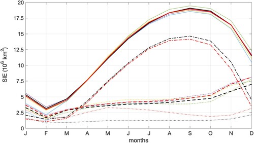
compares GREP (product ref 2.4.1) and CDR (product ref 2.4.2) time evolutions of MIZ and total SIE in four specific months [February (summer extent), May (growing season), September (winter extent) and December (melting season)]. There is a general good agreement between the observational estimates and the ensemble mean. For each month, GREP (product ref 2.4.1) is able to correctly reproduce the amounts of marginal ice and their interannual variability. GREP (product ref 2.4.1) SIE stays always within observational uncertainties. From the melting period to the summer minimum, GREP (product ref 2.4.1) MIZ interannual variability is consistent with satellite estimates, but overestimates MIZ extent indicating overall lower pack ice extent compared to observed data (product ref 2.4.2).

Figure 2.4.3. Time-series of Antarctic SIE (solid) and MIZ extent (dashed) from GREP (red, product ref 2.4.1) and CDR (black, product ref. 2.4.2) for February, May, September, and December. Thin lines represent the single ORAs. An error bar of 10% has been applied to the observational output (product ref. 2.4.2).

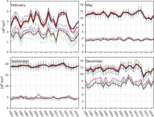
While total SIE (and pack ice extent) ranges from a summer minimum in February (always well under 5 × 10⁶ km²) to a winter maximum in September (always well over 18 × 10⁶ km²) in both GREP (product ref 2.4.1) and CDR (product ref 2.4.2) ( and ), the MIZ presents a minimum in February (generally higher than the minimum pack ice extent), to expand during the growing season when sea ice tends to aggregate and get denser, rapidly increasing the pack ice zone. In September, MIZ comprises about 25% of the total maximum extent but it does not reach its widest extent; it continues to expand toward the end of the year, to exceed again the pack ice extent during the melting season. The fraction of MIZ related to the total SIE is slightly overestimated in December and February by GREP (product ref 2.4.1), to follow more closely observed data in the growing season.

Time evolution of MIZ extent in each month has experienced no or little significant trends for 1993–2020 in both CDR (product ref 2.4.2) and GREP (product ref 2.4.1) – monthly-mean trends are listed in . The reduction in the minimum MIZ extent after 2016 is clearly visible and properly reproduced in GREP (product ref 2.4.1), as the extent increase in 2020. Trends in GREP (product ref 2.4.1) generally follow CDR (product ref 2.4.2). The hemispheric-wide SIE trends for February are negative in both products, driven by the MIZ decrease. During the ice expansion phase (in May), the negative trends in total SIE result from the reduction of the consolidated pack ice. In September, CDR (product ref 2.4.2) and GREP (product ref 2.4.1) exhibit opposing trends in the pack ice and MIZ, they compensate each other to result in a lack of trend in the total extent. During the melting period (in December), negative trends in the pack ice are comparable between the two products, but GREP (product ref 2.4.1) reproduces no trend in the MIZ too, with a larger decline in the total extent.

Table 2.4.1. Slopes of trend lines (computed as linear least-squares regression) for the extent of marginal ice, consolidated pack ice and total ice for February–December (1993–2020) for both GREP (product ref 2.4.1) and CDR (product ref. 2.4.2).

As a consequence of the similarities between CDR (product ref 2.4.2) and GREP (product ref 2.4.1) in estimating total and MIZ extent, the two products agree also in terms of the average locations of the MIZ. We illustrate the MIZ expansion and contraction, and assess the consistency between reanalysis products and observed estimates of MIZ locations, as shown in . There is close agreement in the average latitude changes between the two products. The time evolution of the monthly-averaged position of the MIZ shows that the spatial pattern of the MIZ in GREP (product ref 2.4.1) and CDR (product ref 2.4.2), and its seasonal and interannual variability are again consistent, as well as the timing of MIZ advance and retreat. The location of the minimum MIZ extent slightly moves toward the equator in the last decade, while May and December show a contraction of the MIZ in the most recent years, from 2016. In the growing season, this is mainly due to the reduction of total SIE. The averaged latitude of MIZ is relatively constant in September and persistent at ∼62°S. Although the extent of marginal ice increases until the end of November/December and then its percentage stays nearly constant at this maximum extent, the December-average MIZ position and the outer ice edge move poleward. This is explained by the quick retreat of the inner pack ice starting in the end of September.

Figure 2.4.4. Time series of monthly-averaged latitudes of MIZ for GREP (red, product ref. 2.4.1) and CDR (black, product ref. 2.4.2) in February, May, September, and December.

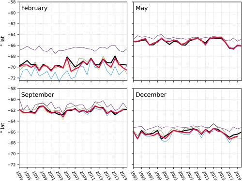
Satellite observations show that the small changes in total Antarctic sea ice over the last three decades mask a dipole pattern of regional changes, with substantial regional trends of increasing ice extent, primarily in the Ross and Weddell Seas, and decreasing ice extent in the Bellingshausen and Amundsen Seas (Parkinson Citation2019). There are complex spatial patterns of change in advance, retreat and duration, forced by wind-driven sea ice drift and ice-ocean heat fluxes. The accuracy of GREP (product ref 2.4.1) performances is investigated also on regional scales using maps of seasonal trends in sea ice concentration during 1993–2020 (). The trends of simulated Antarctic SIC have large spatial differences that greatly agree with observed ice. They both show that the largest trends are present in the regions covered by marginal ice (see contour lines in ). From a seasonal perspective, summer (DJF) and autumn (MAM) have the largest and significant trends in both products. GREP (product ref 2.4.1) SIC exhibits negative trends in the Bellingshausen-Amundsen Sea and in Ross Sea, areas showing rapid regional warming. In summer and autumn, pronounced positive trends occur on the western Weddell Sea and north of the Antarctic Peninsula – they are due to a combination of processes, as changes in the atmospheric dynamics and wind patterns (e.g. Holland and Kwok Citation2012; Meehl et al. Citation2016; Vichi et al. Citation2019; Blanchard-Wrigglesworth et al. Citation2021), changes in the vertical structure of the near-surface water column (Goosse and Zunz Citation2014; Venables and Meredith Citation2014), freezing of low-salinity surface water from the ice sheet (Bintanja et al. Citation2013; Pauling et al. Citation2016; Haid et al. Citation2017). In all regions, the trends start to grow in spring (SON) resulting in the maximum summer trends. In winter (JJA), where the extent of the consolidated pack ice dominates, the largest positive/negative trends are located close to the ice edge (where ice distribution is mostly constrained by ocean dynamics). The spring Antarctic sea ice also shows a zonal wave-number-two structure, with a maximum in the Pacific sector and a minimum close to Davis Station (located on the Ingrid Christensen Coast in East Antarctica), similar to those in spring, except for the difference in the value.

Figure 2.4.5. Map of seasonal trend in sea ice concentration (% yr⁻¹) from CDR (product ref. 2.4.2) and GREP (product ref. 2.4.1) in (a) winter (JJA), (b) spring (SON), (c) summer (DJF), and (d) autumn (MAM), for the 1993–2020 period. Contours indicate the SIC at 0.15 (green) and 0.8 (magenta). Dots show 95% significance. JJA: June-July-August; SON: September-October-November, DJF: December-January-February; MAM: March-April-May.

Figure 2.4.5. Map of seasonal trend in sea ice concentration (% yr−1) from CDR (product ref. 2.4.2) and GREP (product ref. 2.4.1) in (a) winter (JJA), (b) spring (SON), (c) summer (DJF), and (d) autumn (MAM), for the 1993–2020 period. Contours indicate the SIC at 0.15 (green) and 0.8 (magenta). Dots show 95% significance. JJA: June-July-August; SON: September-October-November, DJF: December-January-February; MAM: March-April-May.

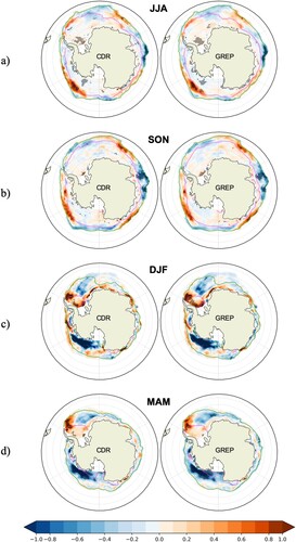
2.4.4. Discussion and conclusions

The region covered by marginal ice is highly sensitive to atmospheric and oceanic forcing, changes in the MIZ extent can affect the level of atmosphere-ocean heat and gas exchanges the area of partially ice-covered ocean and can have implications for the polar ecosystems. Thus, investigation of changes of Antarctic MIZ supports understanding the Antarctic sea ice variability on different spatial and temporal scales.

We have analysed the evolution of the Antarctic MIZ as represented in the Global Reanalysis Ensemble Product (product ref 2.4.1) and compared it to a satellite-derived dataset (product ref 2.4.2). A detailed understanding of mechanisms driving Antarctic sea ice classes is out of the scope of this contribution. Here, we want to assess the reliability of the sea ice concentration provided by the GREP ensemble mean (product ref 2.4.1) in discriminating the MIZ from the consolidated pack ice, and in reproducing the space/time evolution of the Antarctic MIZ from 1993 through 2020.

A challenge in the validation arises as to which long-term sea ice concentration data record to use. There are dozens of algorithms available, whose SICs are not necessarily consistent with each other (e.g. Ivanova et al. Citation2015; Stroeve et al. Citation2016). We derived monthly SIC fields from NOAA and the National Snow and Ice Data Center Climate Data Record (product ref 2.4.2), a long-term, consistent, satellite-based passive microwave record of sea ice concentration that leverages two well-validated concentration algorithms. This data set is not directly included in the data assimilation systems of the GREP (product ref 2.4.1) components.

GREP (product ref 2.4.1) is shown to properly represent the variability of minima and maxima in MIZ extent as well as its interannual variability during the growing and melting seasons. More evident discrepancies between GREP (product ref 2.4.1) and CDR (product ref 2.4.2) occur during summer, when the spread among individual ORA increases: one product tends to underestimate MIZ extent and another to overestimate pack ice extent.

The accuracy of the GREP ensemble mean (product ref 2.4.1) has already been assessed for a range of ocean applications (Storto et al. Citation2019). Although the four reanalyses included in GREP (product ref 2.4.1) employ the same ocean model and atmospheric forcing dataset, differences in ice models, data assimilation systems and observational datasets, air–sea flux formulations, initialisation strategy, and model configuration parameters, contribute to the ensemble dispersion. The ensemble-mean GREP always beats individual members in representing changes in the extent of total and marginal ice, in the Southern Ocean. The quality of GREP (product ref 2.4.1) is comparable to that of satellite data sets and the differences between GREP (product ref 2.4.1) and CDR (product ref 2.4.2) are comparable or even smaller than differences between different algorithms (Stroeve et al. Citation2016).

Nevertheless, the potential of the reanalysis ensemble emerged, but with a list of caveats that might be overcome in future works. The MIZ is very dynamic, making it challenging to provide precise delimitations using monthly SIC that are in turn sensitive to growth/melt processes and air–sea interface conditions. Future investigation of the ice classes variability in GREP (product ref 2.4.1) might benefit from reanalyses and observed values at higher time resolution, and focus on regional changes to better link MIZ extent to dynamical interactions with ocean and atmosphere, and feedback from rapid extreme events on seasonal and sub-seasonal scales. Improvement in data assimilation techniques, space–time data coverage the ice-covered Southern Ocean regions, and availability of other ice properties (such as thickness and drift) from satellite measurements will most probably boost the quality of ORAs and GREP (product ref 2.4.1) in polar regions.

Section 2.5. The Atlantic Meridional Overturning Circulation forcing the mean sea level in the Mediterranean Sea through the Gibraltar transport

Authors: Simona Masina, Nadia Pinardi, Andrea Cipollone, Deep Sankar Banerjee, Vladyslav Lyubartsev, Karina von Schuckmann, Laura Jackson, Romain Escudier, Emanuela Clementi, Ali Aydogdu, Doroteaciro Iovino

Statement and main outcome: Understanding the causes of the variability of the North Atlantic and Mediterranean overturning circulations, and the possible correlation between them is important to disentangle the processes which link the two ocean basins. In this study, we hypothesise that the Gibraltar inflow transport is the main driver of the basin-mean sea surface height variability in the Mediterranean Sea and that they are both anti-correlated to the Atlantic Meridional Overturning Circulation (AMOC) in the North Atlantic.

We analyze here the AMOC and the Mediterranean mean sea surface height (SSH) in an ensemble of eddy-permitting (¼ degree) global ocean reanalyses constrained by observations and historical forcing over the period 1993–2019. Furthermore, we calculate the Gibraltar inflow transport, which is part of the Mediterranean Zonal Overturning Circulation (ZOC) upper branch (Pinardi et al. Citation2019), using the latest release of the 1/24 degree Mediterranean Reanalysis (Escudier et al. Citation2020, Citation2021). In this contribution, firstly we extend the results obtained with observations (2004–2017 period) by Volkov et al. (Citation2019) and confirm the anti-correlation between the Mediterranean mean sea level and the upper branch of the AMOC at 26.5°N over the 1993–2019 period. Secondly, for the first time, we examine the correlation of the different components of the AMOC and the Gibraltar inflow transport and find significant anti-correlations at interannual time scales.

We show that during years of weaker/stronger AMOC and higher/lower SSH in the Mediterranean Sea, a stronger/weaker Azores Current results in stronger/weaker Gibraltar inflow transport. We argue that the direct wind forcing mechanism suggested by Volkov et al. (Citation2019) as a common driver for both the AMOC and the Mediterranean SSH is instead indirect, producing first a changed Gibraltar transport which in turn triggers a change in Mediterranean Sea mean SSH.

Products used:

Table

2.5.1. Introduction

The link between the Atlantic Meridional Overturning Circulation (AMOC) (Marshall and Speer Citation2012; Buckley and Marshall Citation2016; Cessi Citation2019) and the Mediterranean zonal and meridional overturning (Pinardi et al. Citation2019) has been barely discussed in the literature, including modelling studies. This is partially due to the fact that the communities working on the AMOC and the Mediterranean circulation have been so far focused on different aspects.

The overturning circulations in the Atlantic Ocean and the Mediterranean Sea play a key role in setting the stratification of the respective basins and regulating the regional ocean carbon budgets and contribute to the supply of oxygen and other tracers from the surface to the deep ocean (Jaccard and Galbraith Citation2012). Several efforts have been dedicated to the estimate of temporal variability of the AMOC in observations (McCarthy et al. Citation2015 among many), model studies (e.g. Danabasoglu et al. Citation2016) and reanalyses (Jackson et al. Citation2019) due to the AMOC impacts on heat, salt and carbon transports in the Atlantic Ocean and its role in the global coupled climate system (Buckley and Marshall Citation2016). A few aspects of the linkages between the North Atlantic and the Mediterranean Sea intermediate and deep vertical circulation have been investigated, and correlations have been found between the Mediterranean deep-water formation in the Gulf of Lion and the North Atlantic Oscillation (Rixen et al. Citation2005). Other studies have focused on the impact of the Mediterranean Overflow Water (MOW) on the North Atlantic circulation (Swingedouw et al. Citation2009; Ivanovic et al. Citation2014) and the salt content in the Nordic seas (Jia et al. Citation2007). In this study our objective is to investigate the correlations between the AMOC and the Mediterranean Sea circulation on related variables such as the mean sea surface height and the Gibraltar transport.

The mean sea level in the Mediterranean is connected to the Gibraltar net volume transport, water fluxes and air–sea buoyancy fluxes in the Mediterranean Sea (Pinardi et al. Citation2014). Soto-Navarro et al. (Citation2010) estimated a mean net volume transport through Gibraltar of ∼0.04 Sv for the period October 2004 to January 2009. It is the result of the difference between the larger inflow of cold and fresher Atlantic waters (∼0.8 Sv) and the smaller intermediate and deep outflow transports (∼0.76 Sv). These transports are evaluated considering, respectively, the positive (eastward) and negative (westward) zonal velocities integrated along the −5.5°E section. This two-layer flow is connected to the upper and lower branch of the Zonal Overturning Circulation (ZOC) recently described in Pinardi et al. (Citation2019).

Recently, Volkov et al. (Citation2019) found that the AMOC is highly anti-correlated with the mean sea level in the Mediterranean Sea. They suggested the Mediterranean Sea level responds to a mechanism related to an oceanic-gyre-scale change due to the North Atlantic Oscillation (NAO) which modifies the AMOC strength. However, their proposed mechanism correlating AMOC with the Mediterranean mean sea level did not take into account the analysis of the water transport at Gibraltar. In this contribution, we investigate how this mechanism is related to the Azores Current and the Gibraltar inflow transport. Previous works based on observational data provided evidence of the adjustment of the Azores Current to large-scale atmospheric forcing in the North Atlantic (Volkov and Fu Citation2011) and of the exchange through the Gibraltar Strait driven by the Azores Current (Carracedo et al. Citation2014).

Using an ensemble of global and regional reanalyses, we investigate the correlation between AMOC, the sea level in the Mediterranean Sea and the Gibraltar inflow transport. The ability of the global ensemble reanalysis to capture the observed changes from the RAPID array has been already shown (von Schuckman et al. Citation2018; Baker et al. Citation2022, this issue) while the Mediterranean overturning circulation, both in its meridional and zonal components, have only been recently computed (Waldman et al. Citation2018; Pinardi et al. Citation2019; Von Schuckmann et al. Citation2020) but not directly related to the Atlantic counterparts.

In summary, the first objective of this work is to confirm the results obtained by Volkov et al. (Citation2019) using global and regional reanalyses (instead of observations as in Volkov’s paper) and prove that the correlations between the AMOC and sea level in the Mediterranean Sea are still valid over longer time periods (1993–2019 vs 2004–2017). The second objective is to show that the wind-driven mechanism suggested by Volkov to explain the anti-correlation between the AMOC and mean sea level in the Mediterranean Sea is acting to modify the mass inflow transport at Gibraltar mainly due to induced changes in the Azores Current strength.

2.5.2. Methods and data sets

In this paper, we concentrate on the AMOC transport at 26.5°N because the first objective is to reproduce Volkov’s analysis with reanalysis data, verifying that the reanalysis contains the signals identified from observations.

The AMOC transport at 26.5°N is approximately subdivided among three different components (Buckley and Marshall Citation2016): (1) $T_{AMOC} \approx T_{FC} + T_{EK} + T_{UMO}$ (1) where: (i) T_FC is the meridional transport through the Florida strait; (ii) T_EK is the Ekman meridional transport, here calculated from the ERA5 zonal wind stress; (iii) T_UMO is the upper mid-ocean transport down to 1100 m derived at the section between the Bahamas and the western coast of Africa.

In the RAPID estimate of the AMOC transport, the three components of Equation (1) are independently estimated and summed to generate the final transport (Cunningham et al. Citation2007; McCarthy et al. Citation2015). In the following, the same strategy will be used to construct the AMOC transport from the model outputs using the meridional velocities taken from the CMEMS Global Reanalysis Ensemble Product – GREP (product ref. 2.5.2). The calculations are based on the CDFTOOLS diagnostic package (https://github.com/meom-group/CDFTOOLS) and for simplicity we will refer to (1) as RAPID-like decomposition.

The Mean Sea Surface Height (MSSH) over the Mediterranean Sea, MSSH_MS, has been calculated from the GREP outputs as well, with the addition of the steric components, calculated from the GREP temperature (T) and salinity (S) profiles. The MSSH is defined as: (2) $MSS H_{MS} = η_{I} + η_{s} - M_{g}$ (2) where $η_{I}$ is the incompressible component of the sea level, $η_{s}$ is the steric component and $M_{g}$ is the global area average of the monthly mean incompressible and steric components. The brackets indicate the averages in the Mediterranean basin only, normalised by the surface area of the Mediterranean Sea. The steric component is approximated by the density anomaly as follows: (3) $η_{s} \approx - \frac{1}{ρ_{0}} \int_{- H}^{0} δ ρ (T, \bar{S}) d z - \frac{1}{ρ_{0}} \int_{- H}^{0} δ ρ (\bar{T}, S) d z$ (3) where $ρ_{0}$ is the reference sea-water density (1025 kg/m³), the depth H is fixed at 2000 m and the density anomaly is defined with respect to a T, S time mean value, $\bar{T}$ and $\bar{S}$ : (4) $δ ρ (T, \bar{S}) = ρ (T, \bar{S}) - ρ (\bar{T}, \bar{S}) and δ ρ (\bar{T}, S) = ρ (\bar{T}, S) - ρ (\bar{T}, \bar{S})$ (4) Following Pinardi et al. (Citation2014), the sea level tendency can be written as: (5) $\frac{d}{d t} η = - \frac{T_{r}}{Ω} - q_{W} + \frac{d}{d t} η_{s}$ (5) where $T r$ is the net outward transport at Gibraltar, $Ω$ is the Mediterranean Sea surface area and $q_{W} = ⟨ E - P - R ⟩$ is the net freshwater flux at the air–sea interface (E is the evaporation, P the precipitation and R the runoff) and $η = η_{I} + η_{s}$ . Using the definition of the terms in (2), we obtain: (6) $\frac{d}{d t} [M S S H_{M S} + M_{g}] = - \frac{T_{r}}{Ω} - q_{W} + \frac{d}{d t} η_{s}$ (6) The net outward transport at Gibraltar is furthermore given by: (7) $T r = - F_{inflow} + F_{outflow}$ (7) where the Gibraltar inflow transport $F_{inflow}$ is defined as: (8) $F_{inflow} (x, t) = \int_{y_{B_{1}}}^{y_{B_{2}}} \int_{- h}^{0} H [u (x, y, z, t)] u (x, y, z, t) d z d y$ (8) where $x = 5.5 W$ is the longitude of the narrowest part of the Gibraltar Strait, H is a Heaviside step function to process only inflow eastward currents, $h$ is the bottom depth. The $F_{inflow}$ is here calculated from the latest release of the 1/24 of degree Mediterranean Reanalysis (product ref. 2.5.1).

The Gibraltar outflow transport is defined as in (8) but for the westward currents. In conclusion: (9) $\frac{d}{d t} [M S S H_{M S} + M_{g}] = \frac{F_{inflow}}{Ω} - \frac{F_{outflow}}{Ω} - q_{W} + \frac{d}{d t} η_{s}$ (9) Thus, we expect the Gibraltar inflow transport to be correlated with positive tendencies of the mean sea level at the Mediterranean Sea and global scales (the term $M_{g}$ ). We neglect the freshwater flux and the time derivative of the steric component since they have a large seasonal signal that will be subtracted in the present analysis. Furthermore, we neglect the outflow component which is mainly connected to the water mass transformation processes occurring in the Mediterranean Sea on longer time scales.

Pinardi et al. (Citation2019) define the Zonal Overturning Circulation (ZOC) of the Mediterranean Sea connecting the Gibraltar baroclinic transports to the zonal vertical circulation in the upper 600 m, similar to the so-called Wüst circulation (Wüst Citation1961). The $F_{inflow}$ , partially forced by the Atlantic waters and currents, is part of the upper branch of the ZOC and it is expected that a correlation should exist between the vertically integrated transport in the Atlantic, as expressed by T_AMOC, MSSH_MS and $F_{inflow}$ , the latter two being connected by (9).

2.5.3. Results

In (a) we display the monthly time series of MSSH_MS (annual and semi-annual harmonics removed, following Volkov et al. Citation2019), T_AMOC and Gibraltar F_inflow. Their correlations at zero-lag are reported in . The weak T_AMOC events are associated with high MSSH_MS. In particular, the three exceptional events of AMOC minima in 2010, 2011 and 2018 correspond to maxima in MSSH_MS, larger than 5 cm. In general, the anticorrelation between the two variables is particularly strong (−0.45) during the (2004–2017) period (see ), in agreement with the findings of Volkov et al. (Citation2019).

Figure 2.5.1. (a) The T_AMOC (black line), MSSH_MS (annual and semi-annual harmonics removed) (green line) and the Gibraltar inflow transport (red line) over the period 1993–2019. Note that the y axis for the T_AMOC transport is reversed. (b) The 12 month running mean (also detrended) of total T_AMOC (black line), the MSSH_MS averaged in the Mediterranean basin (green line), T_UMO (blue line), T_EK (yellow line) and the Gibraltar inflow transport F_inflow (red line) over the period 1993–2019 (mean and linear trend also removed). Note that the y axis for the AMOC transport is reversed. (c) Lagged correlations between the different components of the T_AMOC, MSSH_MS and the Gibraltar F_inflow over the period 1993–2019. (d) Same as in (c) but for the period used in Volkov et al. (Citation2019): April 2004, Feb 2017. The 95% significance level for correlation is indicated by the dashed grey line (0.37 and 0.51 at zero lag for the longer and shorter period, respectively). Significance level over a 12-month running mean is calculated by assuming one independent degree of freedom per year. Product ref. 2.5.1 is used for the Gibraltar inflow transport, and product ref. 2.5.2 for all the other variables.

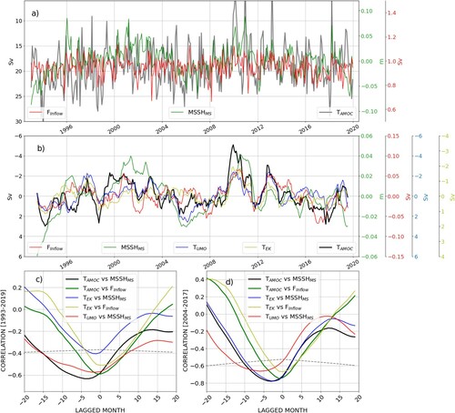
Figure 2.5.2. (Left panel) Correlation coefficients between MSSH_MS, (with annual and semi-annual harmonics removed), the components of the meridional transport at 26.5°N (T_AMOC, T_FC, T_EK, T_UMO) and the Gibraltar inflow transport (F_inflow). (Right panel) Same as in the left panel but between the time series from which annual and semi-annual harmonics have been removed also in the transports. The 95% significance level for the correlation is 0.11 and 0.16 for the longer and shorter period, respectively. Grey solid line (significance) corresponds to the 1993–2019 period, grey dotted line (significance) corresponds to April 2004 – February 2017 period. Product ref. 2.5.1 is used for the Gibraltar inflow transport, and product ref. 2.5.2 for all the other variables.

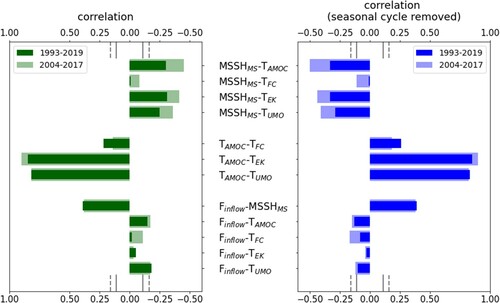
We confirm that the T_EK is the component of the T_AMOC most anti-correlated with MSSH_MS (−0.31 over the whole period and −0.41 from 2004 to 2017, close to the value of −0.43 found by Volkov et al. (Citation2019), see ).

As shown in Volkov et al. (Citation2019), during years of high sea level in the Mediterranean the subtropical and subpolar centres become weaker and shifted southward by about 10 degrees with respect to the climatological mean state. These changes are associated with a southward shift of westerlies, which become more zonal. At the same time, the usually northward Ekman transport at 26.5°N (directed to the right of the wind direction in the Northern Hemisphere) weakened to almost zero and therefore reduced the AMOC transport.

We have done a similar analysis but using the ocean currents and found that during periods when the MSSH_MS is higher than 4 cm the Azores Current strengthens () inducing an increased inflow transport at Gibraltar. In this work we therefore show that the southward shift of westerly winds induces a strengthened Azores Current which induces an increased inflow transport at Gibraltar and, ultimately an increased sea level in the Med Sea.

Figure 2.5.3. Composite currents (amplitude in m/sec in colour) at 75 m depth for the years when the MSSH_MS is >4 cm (panel a) and <−4 cm (panel b). Product ref. 2.5.2 is used.

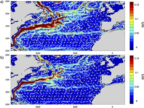
The Gibraltar inflow transport is positively correlated with MSSH_MS and the maximum correlation happens at time lags of a few months (1 month for the period 1993–2019 and 3 months for the period 2004–2017, see ) as expected by equation 9 and suggesting a fast sea level adjustment in the Mediterranean Sea in response to inflow changes at Gibraltar. We argue that the Gibraltar inflow represents the upper branch of the ZOC transport being driven by the mass transport into the Mediterranean Sea through the Gibraltar Strait at monthly and interannual time scales. At longer time scale, other processes are activated, such as water mass transformation in the Mediterranean Sea, which is why we have not used more integrated indicators of the ZOC (such as the maxima of the zonal transport stream function calculated by Pinardi et al. Citation2019).

Figure 2.5.4. (Left panel) Lagged correlation coefficients between MSSH_MS (annual and semi-annual harmonics removed)_, the components of the meridional transport at 26.5°N (T_AMOC, T_FC, T_EK, T_UMO) and the Gibraltar inflow transport (F_inflow). Grey solid line (significance) corresponds to the 1993–2019 period, grey dotted line (significance) corresponds to April 2004 – February 2017 period. The 95% significance level for correlation is 0.37 and 0.51 at zero lag for the longer and shorter period, respectively. Significance level over a 12-month running mean is calculated by assuming one independent degree of freedom per year. (Right panel) Time lags (in month) for which the correlations in the left panel are maxima. Product ref. 2.5.1 is used for the Gibraltar inflow transport, and product ref. 2.5.2 for all the other variables.

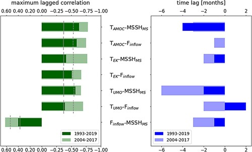
Somehow differently from Volkov et al. (Citation2019), our results indicate that the MSSH_MS is also significantly anti-correlated with T_UMO (−0.25 over the whole period and −0.36 in the 2004–2017 period, see ) at month-to-month time scales. Therefore, our results seem to indicate that the MSSH_MS variability is driven not only by the Ekman induced transport but also by the upper-ocean geostrophic AMOC component. However, we cannot exclude that the different conclusions with respect to Volkov et al. (Citation2019) could partially derive from the different products used.

All the correlations remain basically unchanged when the seasonal cycle (i.e. the annual and semi-annual harmonics) is removed from all the time series, including the transports (right panel of ), suggesting that at zero-lag the relationship between T_AMOC, MSSH_MS and F_inflow is dominated by month-to-month variations.

In order to advance our understanding on the lower frequency co-variability between the AMOC and the Mediterranean Sea zonal overturning, time lagged correlations have been analyzed using 12-month running means of the time series; that is, removing the seasonal and subseasonal variability. In (b), we display the time series of the 12 month running means of the MSSH_MS, T_AMOC, T_UMO, T_EK and F_inflow where the mean and linear trend are also removed. A clear time lagged co-variability starts to emerge at these longer time scales. Over the whole period of analysis, the correlation between the MSSH_MS and the T_AMOC is −0.63, with MSSH_MS lagging behind the T_AMOC by four months (see black line in (c) and ). The lagged correlation is further increased (−0.78) if we consider the latest period (2004–2017), in good agreement with the Volkov et al. (Citation2019) analysis based on observations only, with the only difference being that we find it at 3 months lag while in observations the lag is 6 months, maybe partially due to the different method that we use to filter the seasonal and sub-seasonal variability.

The negative correlation between T_EK and MSSH_MS on interannual time scales is also significant, with the maximum increase with respect to the month-to-month correlation which occurs over the latest period, with the MSSH_MS lagging behind the T_EK by two months (from –0.41 in to −0.77 in ). Over the whole 1993–2019 period the lagged correlation is lower, similarly to what happens to the month-to-month in phase fluctuations. At interannual time scales T_UMO and MSSH_MS are also well anti-correlated in agreement with Volkov et al. (Citation2019). The maximum correlation is −0.57 with the MSSH_MS lagging behind the T_UMO by two months over the whole period. The correlation increases to −0.66 in the most recent period, with the southward/northward anomalies of T_UMO followed by higher/lower sea level anomalies in the Mediterranean six month later (). Volkov et al. (Citation2019) claim that the T_UMO at 26.5°N is related to the zonal difference in pressure and sea level between the eastern and western boundaries of the North Atlantic (see also Wolfe and Cessi Citation2009). In response to a weaker AMOC there is an increased T_UMO (in balance with the zonal pressure gradient) which correlates negatively with the SSH at interannual time scales. They showed that at 26.5°N the upper-midocean transport is correlated with the meridional heat transport. This provides evidence that a reduction of the AMOC, associated with the strengthening of the southward T_UMO, can lead to heat convergence in the equatorial–tropical band and, consequently, rising sea levels along the northwest coast of Africa and ultimately in the Mediterranean Sea. We have reproduced and confirmed some of these results (not shown) even if we found that the time lags between T_UMO and the MSSH_MS is shorter in our case suggesting a faster readjustment process.

At interannual time scales, the Gibraltar inflow transport shows a dramatic increase in the correlation with T_AMOC reaching a maximum (−0.75) over the short period (2004–2017) with the transport lagging three months behind T_AMOC. The correlation remains quite high (−0.53) even over the whole analysis period (see left panel in ). The analysis over the shorter time period shows that both T_UMO and T_EK are significantly anti-correlated with the Gibraltar inflow at different time lags: F_inflow is correlated at zero-time lag with T_EK, while T_UMO precedes F_inflow by two months (see right panel in ). We argue that the North Atlantic wind-driven component of the overturning circulation transport is 180 degree out of phase with the Gibraltar inflow transport at interannual time scales while, as expected, there are a few months delay in the correlation maxima between T_AMOC, T_UMO and F_inflow. This can be understood considering that T_UMO involves the transport on the upper 1100 m water column processes, while F_inflow at Gibraltar is concentrated approximately in the first 150 m of the water column.

2.5.4. Conclusions

In this study, we discuss the connections between the North Atlantic overturning circulation and the Mediterranean Sea mean sea surface height at monthly and interannual time scales through the Gibraltar inflow transport. The usage of the GREP reanalysis product available for the period 1993–2019 allowed us to extend the results obtained by Volkov et al. (Citation2019) with the observational time series at 26.5°N over the shorter period 2004–2017. Our analysis is fully consistent with their results. They showed that the Mediterranean mean sea level, MSSH_MS, is anti-correlated with the upper branch of the Atlantic Meridional Overturning Circulation (AMOC), so-called T_AMOC, and some of its components. When the AMOC transport is small, the mean sea surface height of the Mediterranean Sea is high. In addition, in this work we show that the MSSH_MS is correlated with the Gibraltar inflow transport, F_inflow, which is representative of the upper branch of the Mediterranean Zonal Overturning Circulation.

The novel result here is to show a clear anti-correlation between the T_AMOC and its components with F_inflow at interannual time scales, which has never been discussed before. We argue that the wind-driven induced changes in the North Atlantic are responsible not only for the AMOC variability but largely also for the variability of the Gibraltar inflow transport through Azores Current changes and ultimately to the Mediterranean Sea overturning circulation.

We show that during years of weaker/stronger AMOC and higher/lower SSH in the Mediterranean, stronger/weaker Azores Current reflects into stronger/weaker Gibraltar inflow transport. The direct wind driven mechanism suggested by Volkov et al. (Citation2019) for the AMOC is instead indirect on the Mediterranean Sea mean SSH, producing first a changed Gibraltar transport which in turn produces a change in Mediterranean Sea SSH.

The correlations have maximum values at different time lags, but these depend on the specific time period used for the analysis and we expect these values to have large uncertainties. Limitations to our analysis are inherent to the short time series (1993–2019) since decadal variability cannot be resolved by the 27-year period.

In conclusion, we have connected for the first time the integrated transport of the AMOC with the Mediterranean Sea Gibraltar transport and suggested that the Azores Current plays an important role. We believe this correlation could be of great importance in the future climate scenarios where the North Atlantic is undergoing major changes due to Greenland ice melting and changes in the wind forcing. Future work should consider extending this analysis to longer time series in order to be able to discern the longer time scale correlations.

Section 2.6. Winter fertilization in the Mediterranean Sea euphotic layer and its relationship with Northern Hemisphere large-scale circulation patterns

Authors: Marco Reale, Gianpiero Cossarini, Stefano Salon, Valeria Di Biagio, Anna Teruzzi, Gianluca Coidessa, Emanuela Clementi

Statement of main outcomes: The fertilization of the Mediterranean Sea euphotic layer during winter, as a result, for example, of strong vertical mixing driven by the air–sea interaction, acts in the direction of mitigating the overall oligotrophic state of the basin, influencing at the same time the size distribution of phytoplankton and the food webs in the marine ecosystems of the basin. Here we introduce marine trophic state indicators based on the climatological 90th percentile of daily winter concentration of nutrients to assess locally the potential fertilization of the euphotic layer and its link to Northern Hemisphere large-scale circulation patterns. We found that potential fertilization in the Western (Eastern) Mediterranean is predominantly linked to negative (positive) states of the East Atlantic (East Atlantic/Western Russian) patterns that shape the heat flux losses at the ocean surface and the associated vertical mixing.

Products used:

Table

2.6.1. Introduction

The Mediterranean Sea is widely recognised as an oligotrophic basin (ultra-oligotrophic in the Eastern part), thus characterised by low levels of nutrients concentration (e.g., PO₄ and NO₃) and integrated net primary production compared to the global ocean and a characteristic east–west trophic gradient (Moutin and Raimbault Citation2002; Siokou-Frangou et al. Citation2010; Lazzari et al. Citation2012; Di Biagio et al. Citation2019; Reale et al. Citation2020a). These features result from the overlapping of different physical and biogeochemical processes, such as the anti-estuarine circulation at the Gibraltar Strait, the biological pump in the basin, water column stratification and the spatial distribution of phytoplankton-limiting growth nutrient (e.g. PO₄ and NO₃) sources (Crise et al. Citation1999; Crispi et al. Citation2001; Huertas et al. Citation2012).

In some areas of the basin the oligotrophic state is occasionally mitigated (typically in winter) by the injection of dissolved nutrients in the euphotic layer from the deep waters, as a consequence, for example, of strong mixing mostly driven by heat losses and wind forcing stress acting at the sea surface (Reale et al. Citation2020b). This ‘fertilization’ of the water column in winter acts to favour a decrease of the overall oligotrophy of the basin (Siokou-Frangou et al. Citation2010).

Over the last years, different indicators have been developed to assess the eutrophication of the European regional basins based on satellite-derived 90th percentile of the daily value of chlorophyll-a concentrations (see Gohin et al. Citation2019; Pardo et al. Citation2021 for a review). On the other hand, indicators evaluating the fertilization of the euphotic layer in winter and the relationship between these indicators and the large-scale circulation patterns driving the physical forcing acting on the water column (Josey et al. Citation2011; Papadopoulos et al. Citation2012; Ulbrich et al. Citation2012; Reale et al. Citation2020b) are still poorly investigated. Should this relationship be established, it could pave the way to develop seasonal forecasts of the eutrophication tendency in the basin.

In this work, we first introduce two ‘potential fertilization indicators’, defined in each point of the Mediterranean Sea, for each of the most relevant limiting nutrients for phytoplankton growth (PO₄ and NO₃), based on their climatological daily winter 90th percentile (hereafter: 90th). Secondly, we associate the indicators with the temporal variability of the main Northern Hemisphere large-scale circulation patterns (North Atlantic Oscillation, East Atlantic, East Atlantic/Western Russia and Scandinavian pattern). Thirdly, we discuss the possibility of using the established link to develop seasonal forecasts for the eutrophication tendencies in some areas of the basin.

2.6.2. Materials and methods

We derived the ‘potential fertilization indicators’ for dissolved nutrients in the Mediterranean Sea using 3D daily PO₄ and NO₃ fields provided by the 1999–2019 CMEMS biogeochemical reanalysis at 1/24° horizontal resolution and 125 vertical levels (MEDSEA_MULTIYEAR_BGC_006_008, product reference 2.6.2). The CMEMS biogeochemical reanalysis is produced by the OGSTM-BFM-3DVarBio model (Salon et al. Citation2019; Cossarini et al. Citation2021; Teruzzi et al. Citation2021) coupled off-line with the physical NEMO-OceanVar model (Escudier et al. Citation2021) that is forced with ERA5 atmospheric fields. The biogeochemical reanalysis assimilates surface chlorophyll-a estimates from satellite ocean colour while NEMO-OceanVar model assimilates satellite sea surface height and in-situ profiles of temperature and salinity (MEDSEA_MULTIYEAR_PHY_006_004, product reference 2.6.1). The two reanalyses have been extensively validated (Cossarini et al. Citation2021; Escudier et al. Citation2021) following the CMEMS product quality standard guidelines (Hernandez et al. Citation2018).

Recently, several indicators to assess the eutrophic state of the mid-latitude lakes or ocean basins were developed using different percentile thresholds (75th, 90th, 95th) of the daily values distribution computed for the entire water bodies or locally in each point of the basin (e.g. Poikāne et al. Citation2010; Desmit et al. Citation2018; Gohin et al. Citation2019; Greenwood et al. Citation2019; Brito et al. Citation2020; Pardo et al. Citation2021). Here we use the 90th percentile as a measure of the richness in nutrients or fertilization of the euphotic layer in each point of the domain before the onset of stratified spring conditions, which lead to the phytoplankton blooms. Although arbitrary, the 90th percentile has been chosen in several other studies to characterise the mid-latitude basins eutrophic state (Desmit et al. Citation2018; Gohin et al. Citation2019; Pardo et al. Citation2021).

In order to compute the climatological 90th percentile we first averaged the concentration of both nutrients over the first 100 m of the water column, which can be considered approximately the thickness of the euphotic layer in the basin. Secondly, we considered in each grid point of the domain the 90th percentile of the daily winter concentration of PO₄ and NO₃ (hereafter: 90th_PO4 and 90th_NO3) in the period 1999–2019, where winter corresponds to December, January and February (hereafter: DJF). The 90th percentile threshold is calculated in each point of the basin in order to evaluate the potential fertilization in relation to the local mean trophic level, as recently proposed for local extreme events in Di Biagio et al. (Citation2020).

Then, we defined for each point of the basin a ‘potential fertilization indicator’ for PO₄ and NO₃ (hereafter: FE_PO4 and FE_NO3) as the number of days (not necessarily consecutive) in each winter month of the period 1999–2019 when the value of PO₄ and NO₃ is greater than 90th_PO4 and 90th_NO3, respectively. In this work the term ‘fertilization’ refers to the accumulation of phytoplankton limiting-growth nutrients in the euphotic layer because of different processes acting locally such as input (e.g. vertical mixing, riverine input) or lack of consumption. The higher is the value of the index, the more efficient are these processes to accumulate the dissolved nutrients in the euphotic layer. On the other hand, the adjective ‘potential’ refers to the fact that the presence of high values of nutrients in the euphotic layer is a necessary but not sufficient condition for the development of the phytoplankton blooms. In fact, beside the nutrient content of the euphotic layer, other processes may impact the intensity and temporal evolution of the spring blooms (Mayot et al. Citation2017).

This formulation allows us to investigate whether the highest values of both FE_PO4 and FE_NO3 at each point of the basin could correspond to a particular state of the Northern Hemisphere large-scale atmospheric circulation patterns which shape heat fluxes and, in turn, the vertical mixing in the basin, which is one of the main drivers of the nutrients’ dynamics in the euphotic layer (Josey et al. Citation2011; Papadopoulos et al. Citation2012; Reale et al. Citation2020b).

In this work, in order to characterise the temporal variability of large-scale circulation patterns we use their available monthly indexes that are standardised with respect to the climatology of 1981–2010 (product reference 2.6.3). The large-scale circulation patterns here considered are: North Atlantic Oscillation (NAO), East Atlantic (EA), East Atlantic/Western Russian (EAWR) and Scandinavian pattern (SCAN), which have been widely recognised as important drivers of the physical forcing and of the biogeochemical dynamics of the Mediterranean basin in winter (Josey et al. Citation2011; Papadopoulos et al. Citation2012; Ulbrich et al. Citation2012; Reale et al. Citation2020b).

In order to investigate at which extent the highest monthly values of FE_PO4 and FE_NO3 in each point of the basin correspond to a particular large-scale circulation pattern monthly state, we selected all those winter months when FE_PO4 and FE_NO3 are greater than seven and computed the mean values of the four large-scale circulation patterns indexes for those months (hereafter: SP⁺). The threshold of seven days per month has been chosen after a sensitivity analysis of the statistical significance of the relationship between large-scale circulation patterns and the potential fertilization indicators (not shown).

Finally, we assessed if these values are statistically different from the climatological means of the four indexes during the winter months (SPclim). The statistical significance of the observed difference of the two means have been assessed using a Mann–Whitney test with p < 0.05.

2.6.3. Results

shows the spatial distribution in the Mediterranean Sea of 90th_PO4 and 90th_NO3 percentile in DJF during the period 1999–2019. The distribution is characterised by an east–west/south–north gradient for PO₄/NO₃ whose existence has been already pointed out in previous works (Crise et al. Citation1999; Manca et al. Citation2004; Lazzari et al. Citation2016; Richon et al. Citation2018a, Citation2018b; Di Biagio et al. Citation2019; Richon et al. Citation2019; Reale et al. Citation2020a, Citation2020b). The highest values are observed in the deep convective areas of the basin, namely the Gulf of Lion, Southern Adriatic Sea and the area of Rhodes Gyre (Macias et al. Citation2018b). Moreover, additional strong signals can be found in the Alboran Sea, associated with the coastal upwelling and inflow of Atlantic water at the Gibraltar Strait (Macias et al. Citation2018a), in the Northern Ionian as a consequence of the deepening of the mixed layer depth in the area in winter (D’Ortenzio et al. Citation2005; Lavigne et al. Citation2018), in the area of Northern Tyrrhenian, Pelops and Shikmona gyres (Pinardi et al. Citation2015) and along the coastlines of the basin, for example in the area of Rhone and Ebro river plumes (Western Mediterranean Sea), in the Northern Adriatic Sea (Po river) and in the Levantine basin at the mouth of the Nile river. The Mediterranean riverine inputs are characterised by high values of the N:P ratio (Lazzari et al. 2016), thus explaining the higher NO₃ concentrations near the river mouths which are, at least, more than one order of magnitude greater with respect to what is observed in the case of PO₄.

Figure 2.6.1. Spatial distribution of 90th_PO4 (a) and 90th_NO3 (b) percentile in the Mediterranean Sea in DJF (period 1999–2019). Values in both panels are in mmol/m³ and have been computed using the CMEMS biogeochemical reanalysis (product reference 2.6.2)

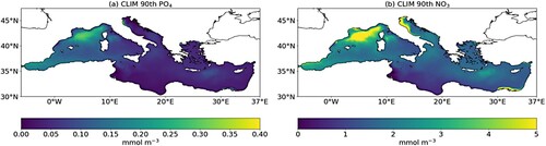
During the winter season, the highest values of FE for both nutrients are observed mainly in February in the offshore areas of the basin when the mixed layer depth in the basin is at its maximum (D’Ortenzio et al. Citation2005; Houpert et al. Citation2015), whilst relatively lower values occur at the river mouths (such as the Po and Nile), in the Gulf of Gabes and in the Alboran Sea. In this case vertical mixing plays a twofold role: (i) it enriches nutrients in the euphotic layer eroding the nutricline; and (ii) it prevents concentration of phytoplankton at the surface by dilution. Moreover, sunlight is minimum during the winter months and thus further limits the phytoplankton capabilities to make the photosynthesis and to consume the available nutrients. (a,b) show the correlation coefficient between the monthly time series of FE_PO4 and FE_NO3 and the monthly time series of the mixed layer depth (during DJF). The highest correlation values are observed in the Gulf of Lion, Tyrrhenian Sea, Southern Adriatic Sea, Northern Ionian Sea, around Crete and in the area of Rhodes, Pelops and Shikmona gyres, confirming the role of vertical mixing in influencing the distribution of nutrients along the water column. On the other hand, in the coastal areas, the correlation coefficients are weak and negative or even not significant, pointing to the importance of river loads in shaping the variability of nutrients in these areas. In fact, relative lower values of FE are observed in the offshores areas of the basin in December, when the nutrient load from the rivers is prevalent with respect to the injection of nutrients in the euphotic zone from the intermediate/deep layer through vertical mixing (not shown).

Figure 2.6.2. Spatial distribution of the correlation between the monthly DJF winter time series of the mixed layer depth and FE_PO4 (a) and FE_NO3 (b) respectively in the period 1999–2019. Only correlation values statistically significant at 95% are shown. Mixed layer depth data are based on the CMEMS physical reanalysis (product reference 2.6.1). FE_PO4 and FE_NO3 have been calculated using the CMEMS biogeochemical reanalysis (product reference 2.6.2).

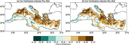
The spatial distribution of the relationship between the winter fertilization indicators and the atmospheric drivers is shown in , which reports, for each grid point, the large-scale circulation pattern with the highest value of the difference between SP⁺ and SPclim for FE_PO4 and FE_NO3.

Figure 2.6.3. Spatial distribution of the highest value of SP⁺-SPclim for PO₄ (a) and NO₃ (b) in the Mediterranean Sea in the period 1999–2019. The size of each dot is equal to the absolute value of SP⁺-SPclim. The large-scale circulation patterns considered are NAO (black), EA (red), EAWR (blue) and SCAN (green). The resolution of the gridded data has been downgraded from 1/24° to 0.5° for sake of clarity. Values have been computed using the time series of the monthly values of the indexes for large-scale circulation patterns (product reference 2.6.3). Only differences statistically significant with p < 0.05 according to a Mann-Withney test are shown.

Figure 2.6.3. Spatial distribution of the highest value of SP+-SPclim for PO4 (a) and NO3 (b) in the Mediterranean Sea in the period 1999–2019. The size of each dot is equal to the absolute value of SP+-SPclim. The large-scale circulation patterns considered are NAO (black), EA (red), EAWR (blue) and SCAN (green). The resolution of the gridded data has been downgraded from 1/24° to 0.5° for sake of clarity. Values have been computed using the time series of the monthly values of the indexes for large-scale circulation patterns (product reference 2.6.3). Only differences statistically significant with p < 0.05 according to a Mann-Withney test are shown.

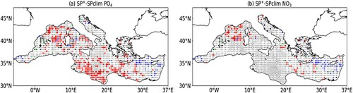
In the case of FE_PO4, EA is the large-scale circulation pattern driving the variability of potential fertilization indicators in the Western Mediterranean Sea (more specifically in the area of the Gulf of Lion, around the Balearic Island and in the Tyrrhenian Sea) and in the Southern Ionian, around Crete and at centre of the Aegean Sea. In the case of FE_NO3, we can again observe the same signal in the Gulf of Lion and around the Balearic Island, while it is weaker in the Aegean Sea and completely absent in the Tyrrhenian Sea and Southern Ionian Sea. Tyrrhenian Sea and Southern Ionian Sea are under the influence of the Middle Tyrrhenian current and Atlantic-Ionian stream which results from the bifurcation of the Atlantic Water entering the Mediterranean Sea at the Gibraltar Strait (Pinardi et al. Citation2015). Thus, it is likely that the boundary conditions set in the Gibraltar Strait play an additional role with respect to the vertical mixing in smearing the variability of FE_NO3 in the two subbasins. The signal related to EA observed in the Western Mediterranean Sea is in agreement with the findings of previous studies that pointed out the importance of EA in shaping the heat fluxes variability over the region and, in turn, the dense water formation processes and nutrient dynamics in the area (Schroeder et al. Citation2010; Josey et al. Citation2011; Reale et al. Citation2020b). Additionally, EAWR also appears to play an important role for both nutrients in the area of the Rhodes gyre and around Cyprus (Josey et al. Citation2011; Reale et al. Citation2020b). No significant relevant signals have been observed in the rest of the basin, in particular in the Southern Adriatic. There, the influence of large-scale circulation patterns is probably masked by the local circulation dynamics (BiOS phenomenon, Gačić et al. Citation2010; Civitarese et al. Citation2010). Moreover, the analysis does not show any relevant signal associated with NAO in the basin, as it is already reported in previous studies (Josey et al. Citation2011; Reale et al. Citation2020b).

shows the slope of the linear regression between the monthly DJF concentration of PO₄ and NO₃ and the EA monthly index. In fact, provided the existence of a link between the intensity of the fertilization and the atmospheric pattern variability, we assessed the magnitude of this link by computing the regression between the monthly nutrient concentration and that particular large-scale circulation pattern monthly index, with the objective to provide a potential seasonal forecast indicator. The highest values of the slope are observed in the Gulf of Lion area and can get up to −0.04 mmol/m³/month and −0.4 mmol/m³/month, respectively for PO₄ and NO₃. The 0–100 m average winter value of PO₄ and NO₃ amount is equal about 0.2 and 2 mmol/m³ respectively, and the monthly variation of nutrient concentration (in %) for a unit of positive monthly index value of EA is nearly equal to 5%. This estimation is consistent with the results provided in Reale et al. (Citation2020b), who considered the extended winter season October-March (for the past period 1961–1999) and observed a total variation of the nutrient concentration ranging between 2% and 3% for a unit of positive EA index value in the same area. Although long-term analysis (Reale et al. Citation2020b) and future projections based on CMIP5 models (Ullmann et al. Citation2014) found no significant tendencies in the EA pattern, the robustness of the link observed mainly in the Gulf of Lion could pave the way to develop seasonal forecasts for the potential fertilization of the area based on the forecast of atmospheric drivers which have become recently available (Lledó et al. Citation2020).

Figure 2.6.4. Spatial distribution of the slope of the linear regression between monthly December-January-February time series of PO₄ (a) and NO₃ (b) and monthly December-January-February EA index time series in the period 1999–2019. Only values statistically significant at 95% are shown. Slopes have been calculated using the CMEMS biogeochemical reanalysis (product reference 2.6.2) and the time series of the monthly values of the indexes for large-scale circulation patterns (product reference 2.6.3)

Figure 2.6.4. Spatial distribution of the slope of the linear regression between monthly December-January-February time series of PO4 (a) and NO3 (b) and monthly December-January-February EA index time series in the period 1999–2019. Only values statistically significant at 95% are shown. Slopes have been calculated using the CMEMS biogeochemical reanalysis (product reference 2.6.2) and the time series of the monthly values of the indexes for large-scale circulation patterns (product reference 2.6.3)

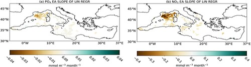
2.6.4. Discussion and conclusions

We introduced an indicator to monitor locally the euphotic layer potential fertilization during the winter season in the Mediterranean Sea and we associated, for each point of the basin, its temporal variability with the large-scale circulation patterns driving the atmospheric circulation over the region. As shown in Di Biagio et al. (Citation2020), the choice of a specific threshold in each point of the basin allowed us to analyze the potential fertilization in relation to the local ecosystem properties. We found a relevant influence of the EA on the fertilization indicators in the Gulf of Lion. In particular, a negative state of EA results in an increase in the nutrients’ concentration in the offshore areas of the Gulf of Lion as well as in the Tyrrhenian Sea, Alboran Sea, Balearic Island, and Southern Ionian Sea (). To a lesser extent, an increase of nutrients’ concentration around the Iberian Peninsula, Sardinia, Gulf of Genoa and Northern Adriatic is related to negative EAWR and positive SCAN states. On the other hand, a positive EAWR state corresponds to higher nutrients‘ concentration in the euphotic layer of the areas around Crete, in the Aegean Sea and the Rhodes Gyre (not shown).

The link observed can be attributed to the importance of EA in shaping the heat fluxes at the surface and thus the vertical mixing along the water column (Josey et al. Citation2011; Papadopoulos et al. Citation2012; Reale et al. Citation2020b). In fact, the vertical mixing acts in such a way to enrich the euphotic layer with nutrients but also to prevent the phytoplankton to concentrate at the surface.

This conclusion is further supported by the spatial distribution of the maximum value of FE_PO4 and FE_NO3 during the winter months of 2020 () which shows a limited fertilization of the euphotic layer of the Mediterranean, in particular in the Northern Western Mediterranean. This limited fertilization appears to be associated with anomalous positive values observed in the EA index in January and February (1.74 and 1.38 respectively).

Figure 2.6.5. Spatial distribution (in number of days) of the maximum monthly value of FE_PO4 (a) and FE_NO3 (b) in the Mediterranean Sea during DJF 2020. Contour lines (with colour legend in the figure) shows the mixed layer depth (in m). Mixed layer depth data are based on the CMEMS physical reanalysis (product reference 2.6.1) FE_PO4 and FE_NO3 have been calculated using the CMEMS biogeochemical reanalysis (product reference 2.6.2).

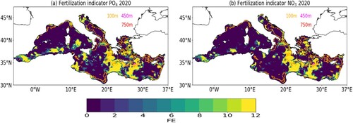
Only limited significant signals are observed in most of the Adriatic Sea and Aegean Sea where the long-term influence of large-scale circulation patterns on the fertilization indicators is probably masked by the substantial nutrient inflow associated with the presence of the Dardanelles Strait (e.g. Aegean Sea, Souvermezoglou et al. Citation2014) and local dynamics such as the BiOS phenomenon (e.g. Adriatic and Ionian Sea, Gačić et al. Citation2010; Civitarese et al. Citation2010).

Although the approach adopted to derive the indicators could strongly benefit from a longer time series to compute the 90th_PO4 and 90th_NO3 percentiles, the preliminary results are promising, because they provided for the first time an overview of the influence of the atmospheric forcing acting over the Mediterranean region on the interannual variability of the local fertilization in the basin measured by the indicators proposed here. Moreover, the approach adopted here is robust, since it uses physical and biogeochemical assimilated datasets which are based on a physical model forced by the high-resolution atmospheric reanalysis ERA5 (Hersbach et al. Citation2020). Although the physical and biogeochemical reanalyses contain uncertainty, as described in Escudier et al. (Citation2021) and Cossarini et al. (Citation2021), the use of data assimilation and of ERA5 forcing can contribute to reduce the errors associated with the model’s parametrization and boundary conditions, also imposing a constraint on the physics and biogeochemistry of the euphotic layer, and thus providing a better representation of their response to the atmospheric forcing acting over the basin.

Being based on the assessment of the links with the Northern Hemisphere large-scale circulation patterns, the present analysis is focused on one of the possible fertilization mechanisms affecting the Mediterranean oligotrophic areas. In fact, additional analysis of the riverine inputs, internal dynamics and local mesoscale and sub-mesoscale processes inducing vertical nutrient transport is needed to better understand the variability of the biogeochemical state and the fertilization effects in the euphotic layer of the Mediterranean Sea.

Acknowledgements

M. Reale has been supported in this work by the project FAIRSEA (Fisheries in the Adriatic Region – a Shared Ecosystem Approach) funded by the 2014–2020 Interreg V-A Italy–Croatia CBC Programme (Standard project ID 10046951).

Section 2.7. Diversity of marine heatwave trends across the Mediterranean Sea over the last decades

Authors: Hugo Dayan, Ronan McAdam, Simona Masina, Sabrina Speich.

Statement of main outcome: Over the past three decades, marine heatwaves (MHWs) in the Mediterranean Sea have caused mass-mortality events in various marine species, and critical losses for seafood industries. MHWs are predicted to become more intense and more frequent under anthropogenic warming, embodying a growing threat to both marine ecosystems and human society. To better understand how global warming has led to changes in these events so far, this study assesses past-to-present variability of MHWs in the Mediterranean Sea. Here, we assess the diversity of marine heatwave trends over 1993–2019 across the Mediterranean Sea. Three different surface temperature products show that the maximum intensity, frequency and duration of MHWs have all increased on average over the Mediterranean Sea since 1993. We show that the means of these metrics display a quite inhomogeneous spatial extent across the Mediterranean Sea over 1993–2019, and the trend of these metrics differ between Mediterranean sub-regions. The differences in the changing behaviours of MHW events, depending on the sub-regions, highlight the need for more local-scale risk-assessments and forecasts.

Product table:

Table

2.7.1. Introduction

In recent years, marine heatwaves (MHWs) – defined as prolonged periods of anomalously high ocean temperature (Hobday et al. Citation2016) – have drawn attention due to their impacts across the global ocean (IPCC Citation2014; Oliver et al. Citation2018, Citation2021). In the Mediterranean Sea, MHWs have caused ecological and economic damage, such as mass-mortality events and critical seafood losses (e.g. in the summer 1999: Cerrano et al. Citation2000; Perez et al. Citation2000; Garrabou et al. Citation2001; Linares et al. Citation2005; in the summer 2003: Garrabou et al. Citation2009; Schiaparelli et al. Citation2007; Diaz-Almela et al. Citation2007; Munari Citation2011; in the summer 2006: Marba and Duarte Citation2010; Kersting et al. Citation2013; and in the summer 2008: Cebrian et al. Citation2011; Huete-Stauffer et al. Citation2011). The record-breaking 2003 MHW affected the Mediterranean sub-regions differently, particularly impacting benthic populations covering tens to thousands of kilometres of coastlines in the western side of the basin (Garrabou et al. Citation2009). Over the 1982–2018 period, the basin-averaged Mediterranean Sea SST has displayed a positive trend of 0.41°C/decade, with more rapid warming in the eastern part than in the western part (0.48°C/decade compared to 0.36°C/decade) (Pisano et al. Citation2020). As a result of this warming, MHWs are predicted to become more intense and more frequent, and embody a growing threat to both marine ecosystems and human society (Oliver et al. Citation2018). In the future, MHWs may undermine the many benefits and services that Mediterranean ecosystems provide, such as food, maintenance of biodiversity, and regulation of air quality (Liquete et al. Citation2016; Martín-López et al. Citation2016).

Despite representing only 0.82% of the global ocean surface area, the Mediterranean Sea is one of the main reservoirs of marine biodiversity, containing between 4% and 18% of the world’s marine species (Bianchi and Morri Citation2000). Generally, abrupt temperature changes can affect the concentration of phytoplankton and, consequently, represent a permanent threat to the biodiversity of marine waters (Colella et al. Citation2016). In the Mediterranean Sea, the western part of the basin is more productive than the extremely oligotrophic (i.e. limited supply of nutrients) eastern side (D’Ortenzio and Ribera d'Alcala Citation2009). As a result, the Ionian and Levantine Sea are much less ‘biodiverse’ than the rest of the Mediterranean Basin (Coll et al. Citation2010). However, a lack of biodiversity, such as in the eastern part of the basin, may cause ecosystem fragility (e.g. Cadotte et al. Citation2012; Mori et al. Citation2013) and potentially greater sensitivity to extreme events for the fewer species that are present. Knowledge of MHW characteristics and the biological context of a target region will be vital in addressing ecological and societal impacts.

Further evaluating past-to-present variability of MHWs is crucial to better understand how global warming has led to changes in these events so far and to predict the heightened local socio-economic risk that they cause. Previous studies of the Mediterranean Sea have covered past MHW trends across the basin (Darmaraki et al. Citation2019a) and in specific areas (Bensoussan et al. Citation2019; Ibrahim et al. Citation2021), as well as predictions of future scenarios (Galli et al. Citation2017; Darmaraki et al. Citation2019b) across the basin. There even exists a MHW tracking website for the region (https://t-mednet.org/t-resources/2020-marine-heatwaves). Galli et al. (Citation2017) explicitly consider the impact on ecosystems by considering MHWs defined by species-relevant temperature thresholds, which is a crucial step for current and future MHW studies. Another way to understand ecosystem impacts of MHWs is to study the trends of MHW characteristics in regions with different levels of biodiversity, and to question how ecosystems in different regions will respond to specific trends. A key contributor to biodiversity is the abundance of phytoplankton biomass (Naeem Citation2012). Phytoplankton is measured indirectly by using chlorophyll (Chl-a) as a proxy (Cullen Citation1982). In the Mediterranean Sea specifically, regions of low biodiversity roughly match regions of low chl-a concentration (Coll et al. Citation2010; Colella et al. Citation2016). Given the heterogeneity in chlorophyll concentrations across the Mediterranean Sea (Colella et al. Citation2016; ), it is necessary to study MHWs across all ‘sections’ of the Mediterranean Sea individually. The ‘sections’ of interest in the Mediterranean Sea should be defined biologically rather than geographically (e.g. Bianchi et al. Citation2012).

Figure 2.7.1. Maps of the 1998–2020 chlorophyll concentration climatology (top) and trend (bottom), provided at 1 km spatial resolution (product ref. 2.7.4). The white lines highlight the borders between the four sub-regions investigated in this study: West (the western Mediterranean Sea); East (the eastern Mediterranean Sea); Adriatic (the Adriatic Sea); Aegean (the Aegean Sea). The trend values are displayed as percentages of the initial value (1998 annual mean) only when significant at the 95% confidence level.

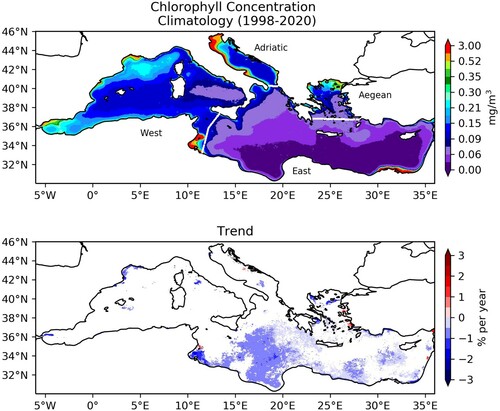
In this study, we explore the diversity of surface MHW trends in sub-regions of the Mediterranean Sea over 1993–2019. To help provide context for future ecological and economic impact studies, we chose to split the Mediterranean Sea into four sub-regions characterised by their distribution of chlorophyll concentrations. We focus on MHW frequency, duration, maximum intensity and category (a measure of the ‘exceptionality’). It is not within the scope of this study to comment on how extreme events have affected productivity. Instead, we highlight that the ecologically-diverse regions in the Mediterranean Sea are each experiencing a different evolution of MHW characteristics. To increase confidence in results, we used three surface temperature records. First, we will present the data and the MHW detection methods (Section 2.7.2). Then, we will discuss the spatial distribution of MHWs trends in each sub-region comparing each dataset (Section 2.7.3). Finally, we will discuss the differences in the changing behaviours of MHWs across the biologically-diverse sub-regions, highlighting potential risks and the need for more local-scale studies.

2.7.2. Materials and methods

In this study, we apply an MHW detection algorithm, described in Hobday et al. (Citation2016) and made available online,Footnote¹ to daily SST datasets. First, we calculate the 90th-percentile for each day of the year over the reference period 1993–2014. Then, percentiles are smoothed with a 31-day moving window average to remove inherent variability. A MHW occurs when the temperature is greater than the 90th-percentile for 5 or more consecutive days. In this study, we apply the algorithm on an individual grid-cell basis. In this paper, we define an ‘event’ as a point wise occurrence of a MHW, instead of an MHW event which is commonly defined using a spatial extent larger than a grid cell. For each grid-cell, the annual number of MHWs and the annual average of duration and maximum intensity (i.e. the highest temperature anomaly during a MHW, with respect to the local climatology for that day of the year) are determined. We also compute the duration for each degree of severity (DS) of a MHW event. DS is defined as the ratio between the SST anomaly with respect to the 90th percentile and the difference between the 90th percentile and the mean climatology. A MHW is defined as moderate if 1 < DS < 2, strong if 2 ≤ DS < 3, severe if 3 ≤ DS < 4 and extreme if DS ≥ 4. Lastly, the annual grid-cell values are averaged within each sub-region to allow for regional trend analysis. We use three state-of-the-art SST datasets, which are freely distributed by CMEMS, to inter-compare the results, and to provide an ensemble approach for the MHW indicators. First, there is a satellite-derived SST record (product ref. 2.7.1) built from Level 3 Advanced Very High Resolution Radiometer (AVHRR) data interpolated onto a 1/20° grid (Buongiorno Nardelli et al. Citation2013; Pisano et al. Citation2016). It has been used to study changes in the Mediterranean Sea over longer periods and with higher resolution than available in earlier satellite-derived climate data records (Pisano et al. Citation2016). Next, the Global ocean Reanalysis Ensemble Product (GREP) is the ensemble mean of four global ocean reanalysis products which use the NEMO ORCA 1/4° grid (product ref. 2.7.2); the major differences between them are in the data assimilation methods and surface forcings used. The ensemble nature of this product allows for an estimate of SST uncertainty, which is very low for Mediterranean SST (Storto et al. Citation2019). Lastly, we also use a high resolution (1/24°) regional model of the Mediterranean Sea (product ref. 2.7.3). Both reanalyses assimilate satellite altimetry and in-situ T-S profiles; all GREP products assimilate SST fields as well, while the regional analysis instead uses SST to correct heat flux. MHWs trends and spatial distributions are studied over the period 1993–2019, which is the longest period common to all datasets (using 1993–2014 as the climatological period).

The 1998–2019 chlorophyll concentration climatology is provided as monthly-averaged fields at 1 km spatial resolution (product ref. 2.7.4). The product is derived from multi-sensor (MODIS-AQUA, NOAA20-VIIRS, NPP-VIIRS, Sentinel3A-OLCI) ocean colour images which are converted to chl-a using a Mediterranean-specific algorithm (Lee et al. Citation2002; Berthon and Zibordi Citation2004; Mélin and Vantrepotte Citation2015; Volpe et al. Citation2007, Citation2019).

2.7.3. Results

We split the Mediterranean Basin into four sub-regions according to biological productivity, using chlorophyll as a proxy (see ). We present our results for each of the metrics comparing the four biological-defined sub-regions of the Mediterranean Sea.

2.7.3.1. Frequency of MHWs

Based on the satellite observations over the period 1993–2019, the number of MHWs showed an inhomogeneous spatial distribution in the entire Mediterranean Sea (between 1 and 3 events; ), with lower number of events per year in the southeastern Mediterranean Sea (between 1 and 2; ) and slightly more events in the western Mediterranean Sea, especially in the northwestern area, as well as the Adriatic Sea (between 2 and 3; ).

Figure 2.7.2. Spatial distribution of the marine heatwave (MHW) metrics from satellite-derived SST record (product ref. 2.7.1) over the period 1993–2019. a, c, e, mean (per year) and b, d, f, trend (per decade) of annual MHW number, MHW duration and MHW maximum intensity. The trend values are displayed only when significant at the 95% confidence level.

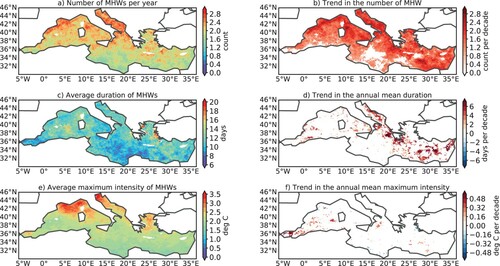
On average, the number of MHWs substantially increased in the whole Mediterranean Sea by approximately 1 event per decade (). The temporal evolution of MHW number per decade agrees very well between high-resolution satellite observations and both the global and regional reanalyses. The linear trend gives a 95% significant interval of 1.08 ± 0.10 MHWs per decade in the satellite observations, compared to about 1.06 ± 0.10 and 1.05 ± 0.10 MHWs per decade in the global and regional reanalyses, respectively ().

Figure 2.7.3. Annual changes (full lines) and linear trends (dashed lines) of MHW metrics averaged over the whole Mediterranean Sea comparing satellite-derived SST record (product ref. 2.7.1) and reanalyses (product 2.7.2 and 2.7.3). a MHW count, b MHW duration and c MHW maximum intensity. Trend values are given with a 95% confidence interval. d, e, f, trend of the MHWs metrics (d frequency per decade, e duration per decade and f maximum intensity per decade) over 1993–2019 for each product and each selected (sub)-region. Purple lines indicate the 95% confidence interval.

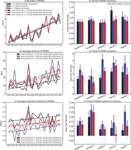
The number of MHWs increased significantly in distinct ways in the four sub-regions. Satellite observations show that the number of MHWs has increased the most in the Adriatic Sea (1.61 ± 0.17 per decade), followed by the Aegean Sea (1.30 ± 0.23 per decade), the western Mediterranean Sea (1.13 ± 0.12 per decade) and finally the eastern Mediterranean Sea (1.01 ± 0.14 per decade; ).

2.7.3.2. Duration of MHWs

Based on the satellite observations over the period 1993–2019, on average, MHWs lasted longer in the Balearic Sea, in the Levantine Basin and in the Aegean southeastern and northwestern coasts (between 10 and 20 days; ), than in the south-eastern Mediterranean Sea, the Alboran and the Adriatic seas (between 6 and 12 days; ).

On average, the duration of MHWs significantly increased in the Levantine Basin, the western Aegean, the Adriatic and the Balearic seas (between 2 and 7 days per decade; ). In the whole Mediterranean Sea the linear trend gives a 95% significant interval of 2.27 ± 0.35 days per decade in the satellite observations, compared to about 3.66 ± 0.65 and 2.79 ± 0.51 days per decade in the global and regional reanalyses, respectively ().

In the biological-defined sub-regions, satellite observations highlight that the duration of MHWs increased the most in the Adriatic Sea (3.36 per decade ± 0.51), followed by the Aegean Sea (3.28 per decade ± 0.86), the eastern Mediterranean Sea (2.41 per decade ± 0.37) and finally the western Mediterranean Sea (2.14 per decade ± 0.56; ).

The duration of moderate MHWs significantly increased in the whole Mediterranean Sea (16.97 ± 1.64 days per decade in satellite observations), compared to the duration of strong MHWs (1.94 ± 0.31 days per decade), severe MHWs (0.15 ± 0.08 days per decade) and extreme MHWs (0.50 ± 0.15 days per decade; ). Satellite observations reveal that the duration of moderate and strong MHWs increased the most in the Adriatic Sea (23.01 days ± 2.67 and 3.22 ± 0.53 days per decade, respectively), while the duration of severe and extreme MHWs increased the most in the Aegean Sea (0.59 ± 0.18 days per decade) and the western Mediterranean Sea (0.53 ± 0.15 days per decade; ), respectively.

Figure 2.7.4. Annual variability (full lines) and trend (dashed lines; trend values are given with a 95% confidence interval) in the duration of MHW in the whole Mediterranean Sea, and e, f, g, h, trend in the duration of MHW for each selected (sub)-region (referred in ), for different degrees of severity (as defined in section 2.7.2). Values compare satellite-derived SST record (product ref. 2.7.1) and reanalyses (product 2.7.2 and 2.7.3). Purple lines indicate the 95% confidence interval.

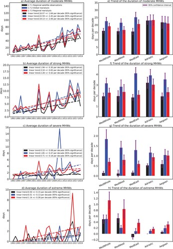
2.7.3.3. Maximum intensity of MHWs

Based on the satellite observations over the period 1993–2019, on average, the maximum intensity of MHWs were stronger in the western Mediterranean Sea, especially in the Gulf of Lion and the Ligurian Sea (more than 3.5°C; ), than elsewhere in the Mediterranean Sea (around 2°C).

The maximum intensity of MHWs significantly increased in the Alboran Sea and the Balearic Sea (between 0.3°C and 0.5°C per decade; ), and to a lesser extent in the Ionian Sea, the Adriatic Sea and the Levantine Sea. It significantly decreased in the Gulf of Sidra (extreme south-eastern Mediterranean Sea) and the Gulf of Lion. Temporal evolution of MHW maximum intensity is well correlated between each product, but biases remain between satellite observations and the reanalysis products (). The linear trend of maximum intensity is overall weak with a 95% significant interval of 0.11 ± 0.04 deg C per decade in the satellite observations, compared to about 0.16 ± 0.04 and 0.12 ± 0.04 deg C in product ref. 2.7.2 and product ref. 2.7.3, respectively.

In the biological-defined sub-regions, satellite observations show that the maximum intensity of MHWs increased the most significantly in the western Mediterranean Sea (0.20 deg C per decade ± 0.06), while it increased very slightly in the Adriatic Sea (0.08deg C per decade ± 0.08), the eastern Mediterranean Sea (0.07 deg C per decade ± 0.03) and the Aegean Sea (0.06 deg C per decade ± 0.06) ().

2.7.4. Conclusion and discussion

In this study, we present 1993–2019 trends of key MHW characteristics for sub-sections of the Mediterranean Sea, defined by their distinct patterns of biological productivity (). These regions are known to have very different levels of biodiversity, and therefore any changes in MHW occurrence will have a different range of impacts. We find that changes in MHW characteristics over the past 27 years are geographically inhomogeneous. Previous studies produced similar statistics on a basin-scale (e.g. Darmaraki et al., Citation2019a; Ibrahim et al. Citation2021), and we also identify increases in MHW frequency, duration and intensity. However, a direct comparison is not possible due to the different reference periods and different MHW thresholds. Interestingly the trend patterns identified here do not directly match the pattern of SST trends in the same time period (Pisano et al. Citation2020), implying that SST trends do not simply translate to equivalent trends in MWH characteristics. The drivers of MHW are therefore more complex, and vary between regions.

Changes in MHW events can affect ecosystem response in the sub-regions differently. For example, the Ionian Sea and the Levantine Basin are the most oligotrophic parts of the basin (), yet the MHWs in each area have evolved differently; the latter is home to more frequent, long-lasting and intense events, while the former is experiencing weaker events. Likewise, the western Adriatic Sea has experienced a greater increase in maximum intensity, while the eastern Adriatic Sea has instead experienced a greater increase in event duration. The Adriatic Sea and the western Mediterranean Sea – areas of rich biodiversity (Coll et al. Citation2010) – have experienced a similar increase in event severity, except that the former has suffered from the most extreme MHWs. This highlights the need for more local-scale risk-assessments, which can benefit from the historical MHW context provided here.

Variability in chl-a concentration in the Mediterranean Sea is typically very high, and there are few regions in the Mediterranean Sea where a significant trend can be detected over the satellite record (). The most notable significant trend shows a chl-a decrease in the eastern Mediterranean Sea (in particular, the Ionian Sea); it is an oligotrophic region which has become even more so since 1998. Coincidentally or not, this overlaps with one of the few parts of the basin in which MHW frequency has not significantly increased (). Likewise, duration and intensity have also experienced little to no increase in this area. It is not known yet if there is a link between changes in extreme warming and biological productivity, yet our results provide motivation to explore this.

This study also acts as an inter-comparison of two reanalysis products against the long-term satellite-derived climate data record. GREP (product 2.7.2) is an ensemble of ¼° reanalyses and acts here as a representative of eddy-permitting resolution, while the high-res regional reanalysis captures finer scale dynamics. The three datasets largely agree on the relative trends between regions (e.g. all datasets suggest the western Mediterranean Sea have the largest maximum intensity trends compared to the other regions), yet the magnitude of these changes varies between the datasets, in particular for GREP. GREP has a tendency to overestimate intensity and duration, as well as the occurrence of higher-category events (though not always outside the confidence intervals of other products). The regional high-resolution reanalysis, meanwhile, typically has MHW statistic values closer to the satellite-derived product. The agreement of the high-res reanalysis and the satellite-derived product implies higher resolution makes an important difference in studying MHWs.

While the datasets agree on the evolution of the duration of moderate and strong events (), there is greater disagreement on the severe and extreme MHWs. For example, the global reanalysis (product ref. 2.7.2) records longer severe events between 2007 and 2019, but none in the early 90s and 2000s. On the other hand the other datasets record severe and extreme events throughout the entire period (1993–2019). while the other datasets record severe and extreme events throughout the record. We note that the datasets have very different resolutions, and therefore different capabilities of incorporating mesoscale and sub-mesoscale drivers of MHWs. The level of agreement found here is nonetheless promising and will allow for further use of reanalyses, which will be necessary for study of the subsurface extent of MHWs and their role in mortality events (Garrabou et al. Citation2019).

The large confidence intervals in the trend calculations (purple ‘error bars’ in and ) are a result of the high variability in MHW characteristics over the past decades. For example, for the maximum intensity in the Adriatic Sea, the trend confidence interval is much larger than in the eastern Mediterranean Sea. Over the period studied, maximum intensity of MHWs is much more variable in the Adriatic Sea and is larger than in the eastern Mediterranean Sea (not shown); this is somewhat expected given the Adriatic Sea’s greater sensitivity to short-term atmospheric variability (Skliris et al. Citation2012; Zveryaev Citation2015).

Each MHW variable helps define potential ecological impacts, but their combined effect is key to a full understanding (Frölicher and Laufkötter Citation2018). For example, it is not known, and may depend on specific species, whether more frequent moderate events are more damaging than rare severe-extreme events. Ideally, datasets would agree on all MHW characteristic trends. However, to comment about the impacts on specific species would require the use of an absolute temperature threshold relevant to that species (e.g. Galli et al. Citation2017). Different species also have complex responses to extreme events, including the ability to recover from brief thermal stress (Hageunauer et al. Citation2013; Thompson et al. Citation2013). A constant barrage of weak events may be more hazardous than a single extreme event (e.g. Pitacco et al. Citation2018), and vice versa. The three datasets used here agree well on the increase in moderate and strong events, yet disagree on the occurrence of severe and extreme events (). The disagreement between datasets on severe MHWs would hinder any analysis on species more susceptible to extraordinary, singular events. This further highlights the need, in future ecological hazard studies, to use more than one product. In the face of climate change and its economic and biological impacts through a substantial increase in a diversity of MHWs, this study can contribute to push towards more research in these areas. In particular, it can support further specific studies to help local policy makers and stakeholders (e.g. aquaculture, fisheries) better identify the regions of the Mediterranean Sea that are strategic for the early implementation of relevant adaptation pathways.

Section 2.8. Long-term interannual changes in extreme winds and waves in the Black Sea

Authors: Joanna Staneva, Marcel Ricker, Adem Akpınar, Arno Behrens, Rianne Giesen, Karina von Schuckmann

Statement of main outcome: This study aims to analyse long-term interannual changes in extreme winds and waves in the Black Sea. Severe wave conditions from 1979 to 2020 are detected using the 99th percentile of the significant wave height (SWH). Long-term spatial wave statistics of the Black Sea are then obtained based on the annual trend of 99th percentile SWH and the number, lifetime, and intensity of extreme events occurring between 1979 and 2020. In addition, the variability of these extreme event characteristics is revealed. Wave reanalysis of the Black Sea is used to investigate intra-annual variation and long-term wave energy potential change. Wave power and wind statistics are shown for the Black Sea CMEMS multiyear products to identify the most suitable areas for wave energy exploitation and offshore wind power potential and to guide the safe and efficient design, installation and operation of marine energy sector assets. The results reveal that the average number of storm events is highest in the eastern basin. In contrast, the average lifetime reaches a maximum on the southwestern coast. Intensity peaks in the same region as the lifetime but is also high in the basin interior. Spatial mean extreme event analyses show a slight increase in event numbers and intensity but decreasing trends for the event lifetime and maximum area of storm events. In regions where wave conditions are strong, there have been increases in extremes relative to normal conditions in recent years. This can significantly affect designs. In terms of wave energy, mean wave power peaks in the southwestern area of the Black Sea. The wave power trend follows a pattern similar to that of the SWH with a pronounced east–west difference; its variation is higher, resulting in a coefficient of variation of ∼2.5.

Products used:

Table

2.8.1. Introduction

In the last decade, the European seas have been hit by severe storms, causing serious damage to offshore infrastructure and coastal zones and drawing public attention to the importance of having reliable and comprehensive wave forecasts/hindcasts, especially during extreme events. In addition, human activities such as the offshore wind power industry, the oil industry, and coastal recreation regularly require climate and operational information on maximum wave height at a high resolution in space and time (Benetazzo et al. Citation2021). Thus, there is a broad consensus that a high-quality wave climatology and predictions and a deep understanding of extreme waves caused by storms could substantially contribute to coastal risk management and protection measures, thereby preventing or minimising human and material damage and losses.

In addition, extreme waves can have serious impacts on the coastal environment and infrastructures (Benetazzo et al. Citation2021). Amarouche et al. (Citation2020) assessed storm events and their potential impacts on the West Mediterranean Sea coasts. The authors found a progressive increase in the number of storm events and their intensity over the last decade and noted the increased damage recently recorded on the Algiers coastlines and the nature of coastal storm damages at the local scale depend on several factors, mainly the power of these storms and their direction given the complex morphology of the Algiers coastlines. Sea state information impacts are directed towards the improvement of the definition of environmental loads over the lifetime of a ship or structure (e.g. wind energy turbines or oil and gas platforms). For example, long-term statistics and high-resolution predictions of SWH are necessary for planning the maintenance operations of offshore wind farms. Subject to wave forecasts, ‘go/no go’ decisions are made on all operations and maintenance activities in offshore wind farms in the days and hours preceding a mission. Indeed, a reduction in the uncertainties of metocean conditions will have a direct impact on structure and mooring loads (both for the ultimate limit state and fatigue design) and on warning criteria for ships. In addition, the design of coastal and offshore structures requires a reliable estimation of extreme wave parameters (Benetazzo et al. Citation2021; Le Traon et al. Citation2021). This information can be obtained through hindcast and forecast studies that apply extreme wave parameters, which are also aimed at expanding the wave CMEMS product catalogue by providing novel wave diagnostics.

Long-term wave statistics for the Black Sea are critical to the safe and efficient design, installation and operation of marine energy sector assets (Akpınar et al. Citation2016). High-resolution regional and coastal wave models can help improve the downscaling of general sea state forecasts, locate hotspots of different wave height properties and correctly prioritise maintenance jobs for offshore wind turbines, reducing their maintenance costs. Applications can further include initial resource assessment (wave power), environmental assessment, and planning (e.g. for installation and execution, operation and maintenance).

Spectral models have made significant improvements over the last decades in predicting bulk wave parameters, such as the SWH, wave periods and directions, and they continue to constitute an essential part of marine weather analysis (Álvarez Fanjul et al. Citation2019; Bingölbali et al. Citation2020; Cavaleri et al. Citation2020). As a result, SWH in the global seas (ECMWF Citation2019) and in the Mediterranean and Black Seas (see, e.g. Arkhipkin et al. Citation2014; Akpınar et al. Citation2016; Sartini et al. Citation2017) has been thoroughly assessed. Studies assessing wave energy potential in the Black Sea have been performed by Rusu (Citation2009), Akpınar and Kömürcü (Citation2012, Citation2013), Rusu (Citation2019), Akpınar et al. (Citation2017, Citation2019), Von Schuckmann et al. (Citation2020), Staneva et al. (Citation2020a), Le Traon et al. (Citation2021), and Bingölbali et al. (Citation2020, Citation2021). Previous studies of the Black Sea mostly focus on mean conditions or individual storms, whereas here, we analyse extreme conditions. Description and statistics of maximum wave parameters (maximum wave height Hm and crest height) of the 1993–2018 climatology of the Black Sea and the Mediterranean Sea in wave models WAM and WAVEWATCH III are shown in Benetazzo et al. (Citation2021) and Le Traon et al. (Citation2021). Here, analyses of extreme wind and wave conditions and wave power statistics are obtained from the recent CMEMS Black Sea long-term wave reanalysis (product ref 2.8.1; Staneva et al. Citation2020b).

2.8.2. Methodology

2.8.2.1. WAM model description

The Black Sea Wave Analysis and Forecasting System is based on the WAM Cycle 6 Black Sea model (spatial resolution of approximately 3 km), which replaced Cycle 4.6.2 (operational since April 2017) within the CMEMS in December 2020 (product ref. 2.8.1; Staneva et al. Citation2020b). The regional wave model for the semi-enclosed Black Sea runs in a shallow water mode with a spatial resolution of approximately 3 km. WAM calculates the two-dimensional energy density spectrum at each of the 44,699 active model grid points in frequency and directional space. The solution of the energy balance equation is provided for 24 directional bands at 15° each, starting at 7.5° and measured clockwise with respect to true north and with 30 frequencies logarithmically spaced from 0.042 to 0.66 Hz at intervals of Δf/f = 0.1. To include the important contribution of higher frequency waves to wave growth/dissipation processes and the output wave characteristics, a parametric tail is fitted for frequencies exceeding the spectral maximum (e.g. WAMDI Citation1988). Detailed descriptions are given by Komen et al. (Citation1994), Janssen and Bidlot (Citation2018), and Staneva et al. (Citation2019). The basic physics and numeric are maintained in the new release. The source function integration scheme developed by Hersbach et al. (Citation2000) and model updates by Bidlot et al. (Citation2007) are incorporated. Wave model performance is discussed in Staneva et al. (Citation2021). The parameterisation of the wave growth in the wind input source term has been adapted to the driving wind fields. The WAM model estimates sea state-dependent momentum and energy fluxes, and Stokes-Coriolis forcing diagnostics are needed to couple to ocean models (Staneva et al. Citation2017). Wave-induced processes have been shown to have a significant impact on drift estimations, e.g. Staneva et al. (Citation2021). WAM cycle 6.0 included the new extreme wave diagnostics (maximal wave height and wave crest, Benetazzo et al. Citation2021) in the new datasets. Wave breaking parameterisation is taken into account, but the time-dependent depth and current fields are not included in Black Sea wave reanalyses (product ref 2.8.1). A novel feature of the Black Sea reanalysis data is that radar altimeter data are assimilated. In addition to SWH, the assimilation includes wind speed data. The required radar altimeter data for this purpose are taken from AVISO (ftp-access.aviso.altimetry.fr; product ref. 2.8.4). The measurements are assimilated into the wave model using an optimal interpolation scheme. Due to a lack of available systematic in situ observations for the Black Sea, satellite data bring added value to wave simulations. The reanalysis simulation covers the period 1 January 1979 to 31 December 2020 (product ref. 2.8.1); that is, in total, trends for 42 years have been simulated with an hourly output time step. Reference Jason-1 data are available for the first period of 15/01/2002 to 21/06/2013, Jason-2 data are available for 22/06/2013 to 30/06/2019 and Jason-3 data are available for 01/07/2019 to 31/12/2019 (product ref. 2.8.4). Making use of the annual time scale provides enough samples to examine quantiles of even higher than the 99th percentile, supporting understanding of peak values in the western part of the Black Sea. A close match of the Black Sea CMEMS data to the satellite measurements for high waves is observed (Von Schuckmann et al. Citation2020).

2.8.2.2. Wind data

The driving forces for the wave model are the hourly ERA5 10-m wind reanalyses of ECMWF (Hersbach et al. Citation2020, product ref. 2.8.2). The quality of ERA5 data for the Black Sea was recently investigated in Çalışır et al. (Citation2021) against altimeter and scatterometer satellite data. It has been shown that ERA5 and Climate Forecast System Reanalysis (CFSR) underestimate wind speeds; however, ERA5 winds have less bias and are more scattered than CFSR winds against the satellite data. Here, wind forcing analyses are performed against the L3 satellite wind observations of METOP-A ASCAT with a spatial resolution of 0.125° (Stoffelen et al. Citation2017; product ref. 2.8.3). The available period of the METOP-A ASCAT data covers 2007–2020 and combines the ascending and descending satellite tracks by using their mean at each time step. To infer statistical quantities, the satellite wind observations are processed as in the ERA5 reanalyses. Changes in extreme ASCAT wind speeds over the Global Ocean are analysed in Giesen and Stoffelen (this issue).

2.8.2.3. Analysis of the storm events

Extreme wave characteristics are studied by analysing single storm events and their long-term means and trends. These storm events were detected using the method proposed by Weisse and Günther (Citation2007). The basis of the method is the definition of a severe event threshold (SET), which we define as the 99th percentile of the SWH ((a)). Then, the exceedance and shortfall of the SWH at every grid point was determined and counted as a storm event ((d)). The time period between each exceedance and shortfall of the SET is the lifetime of an event ((g)). The difference in the maximum SWH of each event and the SET is defined as the event intensity ((j)). The geographic area of storm events and exceedance of the SET are defined as the maximum event area. The number, lifetime, and intensity of events were averaged over the year. Finally, the yearly values were used to compute the long-term means presented in (left column). In addition, for these parameters, we estimated the anomaly of 2020 from the long-term mean (middle column) and the linear trend (right column). To show multiyear variability (), each event, fulfilling the above-described definition, is considered in the statistics. This was done independent of the events’ locations within the domain. To obtain long-term trends, a linear regression was applied to the yearly time series. Trends are computed using the nonparametric Sen's slope estimator for robust linear regression.

Figure 2.8.1. Long-term wave statistics of the Black Sea. Significant wave height (a) 1979–2019 99th percentile, (b) 2020 99th percentile anomaly, and (c) 1979–2020 linear trend of 99th percentile. (d), (g), and (j) yearly average number of storm events, (e), (h), and (k) lifetime of storm events, and (f), (i), and (l) intensity of storm events for the same periods as in (a)-(c). The analyses are based on yearly averages obtained from product ref. 2.8.1.

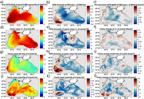
Figure 2.8.2. Long-term wind statistics of the Black Sea obtained from the METOP-A satellite (upper row; product ref. 2.8.3) as well as ERA5 (lower row; product ref. 2.8.2). The considered periods start in 2007 and 1979, respectively. (a) and (d) 99th percentile until 2019, (b) and (e) 2020 99th percentile anomaly, and (c) and (f) linear trend of 99th percentile until 2020. The analyses are based on yearly averages.

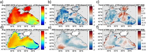
2.8.2.4. Wave power characterisation

The wave power was obtained as a prognostic model output using the following formula: $P = \frac{ρ g^{2}}{64 π} H_{s}^{2} T_{e} \approx 0.48 H_{s}^{2} T_{e},$ where ρ is water density, g is acceleration due to gravity, Hs is the significant wave height, and Te is the wave energy period. A variety of standard statistics, such as the standard deviation, specific percentiles, and the maximum were determined as yearly averages. In addition, the Coefficient of Variation (CoV) was computed and is defined as the standard deviation divided by the long-term mean.

2.8.3. Results

Long-term wave statistics of the Black Sea were derived by considering three important features (the mean, the 2020 anomaly, and the linear trend) of four characteristics described in the previous section (the 99th percentile SWH, yearly average number, lifetime, and intensity of storm events), and the results are presented in . The 99th SWH mean percentile for 1979–2019 ((a)) shows a similar pattern to that of previous analyses using the CMEMS wave products (Álvarez Fanjul et al. Citation2019; Staneva et al. Citation2020a), demonstrating that the highest values of the mean annual 99th percentile, above 3.5 m, occur in the western Black Sea, while the 99th percentile values of the eastern part of the basin are approximately 2.5 m. This pattern is also consistent with previous studies (Akpınar et al. Citation2016 and Van Vledder and Akpinar Citation2016). The anomaly of the 99th percentile for 2020 is mostly negative ((b)); the highest positive anomalies of the 99th percentile for 2020 (ca. 60 cm) are located in the southwestern section of the Black Sea. This result correlates well with the anomaly of the wind speed for 2020 (). The yearly mean lifetime of storm events ((g)) reached maximum values (approximately 20 h) in and around Burgas Bay and reached values of over 15 h in the coastal part of the southwestern Black Sea from the Gulf of Kavarna to Bosphorus. In the remaining areas, the average annual lifetime of storm events exceeds 7.5 h. (d) also shows that the yearly mean number of storm events is low in regions where the average annual lifetime and intensity of storms are high. In contrast, the number of events is high where their lifetime and intensity are low. The mean intensity of the events ((j)) reaches the highest values (approximately 1 m) in the Bosphorus and Sakarya canyons in the southwestern area of the Black Sea. While the southwest Black Sea is exposed to yearly mean storm event numbers of below the long-term averages ((d)), it is observed that the yearly mean lifetime of the events in the same region is higher than the long-term averages ((g)). As expected, the extreme wave statistics based on the 99th percentile threshold of the SWH are very similar to the wind sea wave parameter, and the swell contribution is much lower (not shown here). In terms of the mean intensity of events, in 2020, more severe waves occurred in the coastal region between Bosphorus and Burgas Bay and in the region narrowing and extending from this region to the open waters, more than 1 m over the long-term average ((k)). This in part explains the damage that has occurred in these regions in recent years.

To visualise the time behaviour of the wave extremes, we show spatially averaged 42-year time series of the number, lifetime, and intensity of extreme events (). Extreme wave heights were validated against the observations given in Staneva et al. (Citation2020a). Over the entire period, the number and intensity of events increased, while the lifetime and area of extreme events slightly decreased. This long-term development can be decomposed into a decrease in the frequency of severe wave events from 1979 until 1986, an increase between 2000–2005 and 2011–2016 and an attenuation in the intensity and duration of these events from approximately 2002–2010. This development is mainly due to the wind sea waves. In recent years, trends in the number of severe wave events closely correspond to the reported evolution of the annual 99th percentile of the SWH (Staneva et al. Citation2020a).

Figure 2.8.3. Yearly (a) number, (b) lifetime, (d) intensity, and (f) maximum event area. The dashed lines denote the linear regression (c), (e), and (g) are the respective histograms. The histograms have the following bin sizes: 5 h, 0.1 m, 0.05 km², respectively. The analyses take into account the whole model domain and are based on product ref. 2.8.1. Long-term spatial mean storm analyses of the Black Sea based on 42-year CMEMS wave reanalyses show almost no trend in event numbers (0.029 ± 0.275 events/year), a slight increase of their intensity (0.774 ± 2.938 cm/year) but decreasing trends in the event lifetime (−0.021 ± 0.061 h/year) and event area of extremes (−5.903 ± 169.676 km²/year).

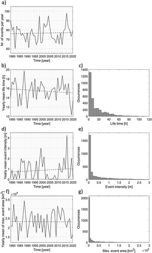
We also analyse the linear trends of 1979–2020 for different severe wave event characteristics. The SWH trend for 1979–2020 reveals an east–west difference with a dominant negative difference in the western region and a positive difference in the eastern region (not shown here). Along the western and southwestern coasts, the trend of the 99th percentile of the SWH is positive ((c)). Notably, this is also the area where the mean lifetime of events reaches a maximum ((h)). The yearly change in the frequency of events is positive overall except along the Crimean Peninsula and in the southern Black Sea ((f)). In contrast, the lifetime trend ((i)) is mostly negative (−10 min/year), and only in some areas along the northwestern and southern coasts and the eastern Black Sea is the lifetime of extreme events increasing. Along the southwestern Black Sea coast, the yearly mean lifetime and intensity of events reach their maxima, while the number of events is small relative to the rest of the basin. The analyses show that in the regions where wave conditions are strong, there have been increases in extremes relative to normal conditions in recent years. This can significantly affect designs for infrastructure.

Figure 2.8.4. Long-term wave power statistics of the Black Sea. (a) 1979–2019 99th percentile, (b) 2020 99th percentile anomaly, and (c) 1979–2020 linear trend of 99th percentile. (d) Standard deviation, (e) maximum, and (f) coefficient of variation of the period 1979–2020. The analyses are based on yearly averages derived from product ref. 2.8.1.

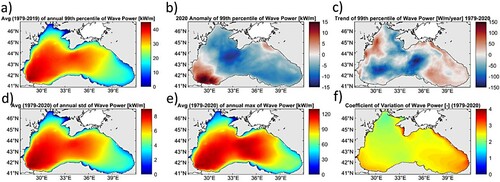
It can be inferred that the increase in the 99th percentile SWH in the southeastern part of the model domain is mainly caused by an increase in the number of extreme events, whereas their duration shows no significant change. Along the southwestern coast, all extreme statistics show a positive trend. In contrast, in the central Black Sea, there were no significant changes in the number of severe events, whereas the average duration of extreme events exhibited a slightly negative trend of up to 5 min/year, which was probably caused by wind changes. In summary, the analyses show that the average number of storm events is the highest in the eastern basin. In contrast, the average lifetime reaches its maximum on the southwestern coast. The intensity reaches its maximum in the same region as the lifetime but is also high in the basin interior. The different causes of the described changes in extreme wave climate may have implications for different applications. For example, coastal marine constructions (e.g. levees) are likely to be more sensitive to the duration than to the number of extreme wave events, whereas for navigation, the number of days with no or only restricted services due to heavy seas may be an issue.

The 99th percentiles of wave power mean patterns for 1979–2020 are overall consistent with the SWH ((a), and Staneva et al. Citation2020a). The spatial pattern of mean annual wave power echoes the findings of Valchev et al. (Citation2013), Rusu (Citation2019), and Akpınar et al. (Citation2017). The maximum 99th percentile of wave power is observed in the southwestern Black Sea. There are hardly any changes in wave power in the southeastern Black Sea (Figure 2.8.5(c)). The changes in wave power are positive in surrounding areas of the Danube Delta and along the western Black Sea coast. A slight and nonsignificant increasing trend is observed along the eastern Black Sea coastal areas. Offshore in the central Black Sea and west of the Crimean Peninsula, the 99th percentile of the wave power trend is decreasing. The pattern of the anomaly of the 99th percentile of wave power in 2020 (2.8.4b) correlates well with that of the wind speed anomaly in 2020 (), revealing a positive wave-power anomaly in the southwestern Black Sea and a negative anomaly in the central basin.

The long-term variability of the mean wave energy potential is critical for the wave energy sector. The overall economic profitability of a given site can be evaluated in terms of average energy production taking into account its distribution over wave heights, periods and directions. A significant factor in this evaluation is interannual fluctuation, demonstrated here with the mean pattern of the coefficient of variation ((f)). A lower variation coefficient, in combination with sufficiently high wave energy flux, can indicate that a specific area is promising for a stable wave energy production. The Crimean coast and the area along eastern coastline show to be the most pronounced inter-annual variability. It is important to notice here that in the regions with the highest average wave power, the inter-annual variability is relatively low. On the north-western shelf and along the southern coast the variability is very low.

2.8.4. Discussion and conclusions

Long-term changes in extreme wave conditions are difficult to detect and to analyse because of the rare occurrence of these events as well as their limited spatial and temporal extent. Analyses of long-term changes require long and homogeneous time series that cover the area of interest at high spatial and temporal detail, a requirement that is frequently not fulfilled by the available observational data. Wave reanalysis data produced by wave model simulations together with data assimilation have therefore become a common tool to complement existing observations and to analyse trends and variability of severe wave events at different scales (e.g. ERA-5 wave analyses, CMEMS products). Here we used a recent CMEMS wave reanalysis (Staneva et al. Citation2020b) for the Black Sea covering the past 42 years (1979–2020). The reanalysis are produced using the: (1) WAM Cycle 6.0 state-of-the-art wave model that includes new dissipation term parameterisations introduced by Ardhuin et al. (Citation2010) and ECMWF (Citation2020), (2) switching to highfrequency atmospheric analyses data of ECMWF ERA-5 and data assimilation of along-track SWH observations, (3) using satellite observation data assimilation The time evolution of the percentile-based storm indices closely follows that described for the 99th percentile of the significant wave height in the Black Sea area.

The major findings are as follows:

The average number of storm events is the highest in the eastern basin. In contrast, the average life time has its maximum at the southwestern coast. The Intensity has its maximum in the same region as the life time but is also high in the basin interior.
The different causes of the described changes in extreme wave climate may have different implications for different applications. For example, coastal marine constructions (e.g. levees) are likely to be more sensitive to the duration than to the number of extreme wave events, whereas for the navigations the number of days with no or only restricted services because of heavy seas may be an issue.
The impact statistics for events show no significant trends on the Black Sea basin scales. Only the 99th percentile trend is slightly negative.
The storm analyses show that the yearly average number of storm events is the highest in the eastern basin. In contrast, the average life time has its maximum at the southwestern coast. The intensity has its maximum in the same region as the life time but is also high in the basin interior.
Long-term spatial mean storm analyses for the Black Sea show based on the 42-year CMEMS reanalyses show slight increase of event numbers and intensity, but decreasing trends for event life time and maximum area.
The mean wave power has its maximum in the southwest of the Black Sea. Compared to the mean wave heights, its variation is much higher resulting in a CoV of ∼2.5 (∼0.75 for mean wave height). The wave power trend has a similar pattern compared to the one of the wave height with a pronounced east–west difference.

In the agreement signed between MOI and the ‘European Commission’ is stated that future Copernicus Marine Service will ‘aim to better support EU policies and directives, increase its user base beyond Europe and in emerging blue markets such as ocean energy, desalinisation or blue biotechnology and infrastructure (see the Blue Economy report 2021)’. The study here contributed to the ocean energy sector. We propose new OMIs that are the trend of the frequency and lifetime of the events and the CoV of wave power.

Funding

This research was funded by the Copernicus Marine Environment Monitoring Service for the Black Sea Monitoring and Forecasting Center (Contract 21002L4-COP-MFC BS-5400) and the EU H2020 Project ‘Developing Optimal and Open Research Support for the Black Sea’ (DOORS), grand agreement: 101000518.

Section 2.9. The Black Sea overturning circulation and its indicator of change

Authors: Mehmet Ilicak, Salvatore Causio, Stefania Ciliberti, Giovanni Coppini, Leonardo Lima, Ali Aydogdu, Diana Azevedo, Rita Lecci, Derin U. Cetin, Simona Masina, Elisaveta Peneva, Murat Gunduz, Nadia Pinardi

Statement of the main outcome: The Black Sea (BS) is the largest deep estuarine basin in the world. Its meridional overturning circulation (BS-MOC) is here described for the first time: in particular, the BS-MOC interannual variability in both depth and density space has been computed using a state-of-the-art ocean reanalysis provided in the framework of the Copernicus Marine Service for the Black Sea of 28 year-period (1993–2020) for the definition of a new climate index. The mean meridional streamfunction defined for the upper 150 m in the depth space reveals an anticlockwise cell in the southern part of the Black Sea coming from the injection of the Mediterranean waters through the Bosphorus Strait into the Black Sea and a clockwise cell in the northern part of the Black Sea as a manifestation of the Cold Intermediate Layer (CIL). The new index is then defined as maximum overturning circulation in density space between 22.45 and 23.85 kg m⁻³. For the overall period, the BS-MOC index weakened between 1993 and 2010 from 0.13 Sv down to 0.07 Sv, then it recovered and has equilibrated around 0.1 Sv. Additionally, it shows a very strong correlation with the CIL from observational data, supporting the concept of using such an indicator to understand and monitor the water mass formation in the Black Sea basin.

Product used:

Table

2.9.1. Introduction

The Black Sea is the largest deep estuarine basin in the world with a large shelf in the North-Western region dominated by the Danube River outflow. It interacts with the Mediterranean Sea through the Turkish Strait System, consisting of the Dardanelles Strait, the Marmara Sea, and the Bosphorus Strait. The warm and salty Mediterranean waters flow onto the Marmara Sea and enter the Black Sea. Then, the Black Sea exchanges its fresh and cold waters with the Mediterranean Water. A cyclonic circulation pattern (aka the Black Sea Rim Current) characterises the water mass circulation in the Black Sea leading isopycnals to rise in the central basin and depress over the continental slope (Oguz et al. Citation1993). A two-layer vertical structure due to salinity difference between the upper 250 m and deep part of the Black Sea limits the vertical motion. The Cold Intermediate Layer (CIL) is the intermediate water mass formation in the Black Sea. It forms on the vast continental shelf in the north, and ventilates the subsurface waters (up to 200–250 m). Strong atmospheric forcing in some winters combined with freshwater inputs induce formation of the CIL in the Black Sea, which regulates the vertical stratification, giving an indication on the thermohaline variability in the upper and intermediate waters. Below approximately 200 m, the Black Sea becomes homogeneous and anoxic, preventing marine life at all. The CIL and inflow of the Mediterranean Water (MW) flowing from the Bosphorus Strait are the main processes which ventilate the subsurface of the Black Sea (Özsoy et al. Citation1993; Özsoy and Ünlüata Citation1997). There is already some evidence of the recent environmental changes in the Black Sea due to anthropogenic climate change (Stanev et al. Citation2019; Capet et al. Citation2020). Observations show that the CIL has been disappearing over the last two decades. Understanding the impacts of changes of water mass properties such as the CIL and MW on the Black Sea circulation still remains a challenge.

Meridional overturning circulation (MOC) systems in the Atlantic and Mediterranean Sea are very crucial to setting the stratification in these basins (Cessi Citation2019). Generally, the MOC depends on intermediate and bottom water formation and their upwelling processes as a part of the ventilation of the basin. Although the Black Sea overturning is smaller than the Atlantic MOC and Mediterranean Sea overturning, we still believe it contains important information about the evolution of the intermediate water masses in the Black Sea. The proposed index could potentially be used to monitor decadal signals of the ecosystem health of the Black Sea due to anthropogenic induced climate change.

Previously, the deep circulation of the Black Sea has been studied using the barotropic stream function (Stanev Citation1990; Stanev et al. Citation2004), however to our knowledge the meridional overturning circulation has not been analyzed yet. Our aim in this study is to describe the time mean and evolution of the meridional overturning system in the Black Sea using an eddy-resolving model that assimilates an observational dataset. This is a unique opportunity since the Black Sea basin is significantly different from the Mediterranean Sea and Atlantic Ocean since the Black Sea basin is much closer to satisfying the so-called ‘horizontal convection’ theorem. Sandström (Citation1908, Citation1916) stated that there cannot be a sustainable circulation when the heating is at the level of the cooling source in a closed basin. Although, this ‘postulation’ is later proven wrong by numerical studies and lab experiments especially if there is a bottom-reaching deep convection (Coman et al. Citation2006; Scotti and White Citation2011), there is still evidence that an idealised overturning circulation should be weak and shallow (Ilıcak and Vallis Citation2012) provided that there is no additional mixing (such as due to internal tides and winds). The background diapycnal diffusivity in the Black Sea is an order of magnitude lower than its counterpart in the Atlantic Ocean (10⁻⁵ m²/s, Ledwell et al. Citation1998). This is probably due to a lack of tidal mixing over rough topography and deep water formation in the Black Sea. Thus, our hypothesis is that the MOC in the Black Sea should be smaller and shallower than the aforementioned larger basins. Our aim is to describe the interannual variability of the Black Sea overturning system using a state-of-the-art reanalysis ocean model simulation and try to understand the Black Sea intermediate water formation and ventilation mechanisms with newly developed meridional overturning index. The main reason undertaking the present study is to develop an index that is possible to assess a future climate change on the Black Sea circulation. The overturning index that gives information about surface, sub-surface and deep ocean circulation is unique. Therefore, this new index will trace possible buoyancy forcing changes in terms of the Bosphorus Strait inflow, river runoff into the Black Sea and sea surface temperature increase trend, and their impact onto the circulation.

2.9.2. Data and methods

The multi-year dataset used in this work is the CMEMS reanalysis for the Black Sea (BS-REA hereinafter, Lima et al. Citation2021, product ref. 2.9.1), which provided daily and monthly mean fields spanning 28 years of integration time from 1993 to 2020 (Lima et al. Citation2020). BS-REA is based on the NEMO v3.6 ocean general circulation model (Madec Citation2016) at the horizontal resolution of 1/36° × 1/27° and 31 vertical levels with partial steps. It is forced by ECMWF ERA5 atmospheric reanalysis fields at the horizontal resolution of 0.25° and 1-hour frequency in time. The model implements a closed boundary condition at the Bosporus Strait with damping of the vertical distribution of temperature and salinity at the Bosphorus Strait exit using the solution provided by a high-resolution unstructured model for the Marmara Sea (Aydogdu et al. Citation2018). The model is online coupled with OceanVar (Dobricic and Pinardi Citation2008; Storto et al. Citation2011), a 3D-Var scheme for the assimilation of in situ temperature and salinity quality-controlled profiles provided by CMEMS INS TAC and historical SeaDataNet and along track sea level anomaly satellite data provided by CMEMS SL TAC. The model solution is relaxed to sea surface temperature satellite data (product ref. 2.9.4) provided also by CMEMS.

To understand the overturning circulation of the Black Sea, we compute the time-mean meridional Eulerian (overturning stream function in the geopotential coordinate) and residual (overturning stream function in the density ( $σ_{2}$ ) coordinate) stream functions according to Pinardi et al. (Citation2019).

The Eulerian meridional stream function $Ψ$ is defined as function of latitude and depth, and calculated by integrating the meridional velocity as follows: $Ψ (y, z) \equiv - \frac{1}{T} \int_{t_{o}}^{t_{1}} \int_{x_{B 1}}^{x_{B 2}} \int_{- H}^{z} v (x, y, \tilde{z}, t) d \tilde{z} d x d t$ where $x_{B}$ is the meridional (east–west) boundary, T is the temporal averaging interval and H is the bottom bathymetry. Positive (negative) values represent clockwise (anticlockwise) circulation along the vertical direction. We also use residual stream function $Ψ^{*}$ in the density space ( $σ_{2}$ ) as follows: where $H$ is the Heaviside function. We used 100 density bins to remap the mass flux fields to compute the residual stream function.

2.9.3. Results and discussion

The time mean meridional Eulerian and residual stream functions for the Black Sea were evaluated for the entire BS-REA simulation period (1993–2020) for the whole basin. (a) shows the time-mean Eularian meridional overturning stream function, and three different isopycnal layers (22.45, 23.85, 25.7 kg/m³) as dashed lines in the Black Sea. We will discuss the importance of these isopycnals in the next section. Upward doming isopycnals indicate strong cyclonic circulation over the continental shelf (Rim Current). Note that the depth axis is non-linear. There is an anticlockwise (negative) circulation in the southern part of the Black Sea (south of 44°N) and a clockwise (positive) circulation centred around of 44.5°N at the upper 150 m. This surface circulation is a manifestation of the CIL coming from the continental shelves in the north and injection of the Bosphorus Strait water in the south. Observations show wider range for the penetration of the Bosphorus Strait overflow into the Black Sea (around 100–500 m, Özsoy et al. Citation1993; Özsoy and Beșiktepe Citation1995), but z-coordinate models generally suffer from additional numerical mixing which leads to shallower equilibrium depth for the gravity currents (Ilıcak et al. Citation2012). In the abyssal basin, there are three different cells; one of them is negative (anticlockwise), and the other two are positive (clockwise) cells. The time-mean values of these different cells are approximately around 0.1 Sv, however, day to day changes can be up to 5 Sv (not shown).

Figure 2.9.1. Time-mean Eulerian meridional overturning maximum of the absolute value of the stream function (isopycnal layers 22.45, 23.85, 25.7 kg m⁻³ as dashed lines) on the top; yearly maximum overturning stream function for the whole basin (blue line) and down to 250 m (red line) on the bottom with standard deviations as the bar plots.

Figure 2.9.1. Time-mean Eulerian meridional overturning maximum of the absolute value of the stream function (isopycnal layers 22.45, 23.85, 25.7 kg m−3 as dashed lines) on the top; yearly maximum overturning stream function for the whole basin (blue line) and down to 250 m (red line) on the bottom with standard deviations as the bar plots.

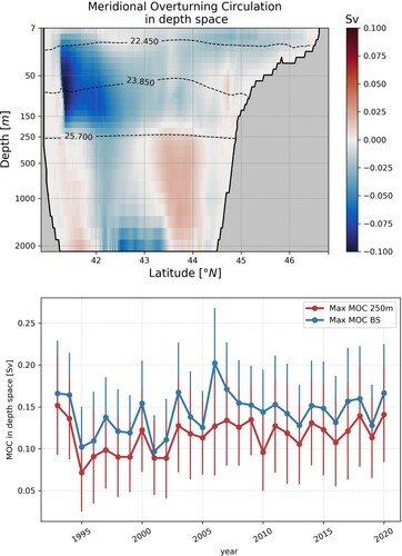
The yearly maximum meridional overturning stream function down to 250 m (red line) and the whole basin (blue line) and their respective standard deviations were computed between 1993 and 2020 and are shown in (b). There is a weakening in BS-MOC from 0.17 to 0.1 Sv in the first three years of the integration time (1993–1995), then there is an increasing trend between 1995 and 2005 in both BS-MOC values. After 2005, the BS-MOC values saturate with a mean of 0.114 and 0.142 Sv for the upper 250 m and the whole basin respectively over the rest of the simulation period. The correlation between maximum BS-MOC at the upper 250 m and the whole basin is very high (Pearson correlation coefficient, r = 0.83). High correlation between upper and whole basin BS-MOC strength indicates that the flow can be barotropic, and the bottom cell (below 250 m) is stronger than the upper cell.

Next, net meridional transports are computed in potential density anomaly with reference pressure of 2000 dbar ( $σ_{2}$ ) space. We believe that the MOC function of density better characterises water mass transports in the Black Sea than the MOC function of depth. (a) shows the time-mean overturning transport computed in density space. The Mediterranean Water coming from the Bosphorus Strait is the densest in the whole basin due to highly saline water coming from the Mediterranean Sea. There is an anticyclonic circulation at the density values larger than 26.5 kg m⁻³, indicating the Mediterranean Water injection. There are two dipole (positive–negative) circulations at two different density bins between 26.05 and 26.35 kg m⁻³. These two circulations correspond to the three deep cells in the $Ψ (y, z)$ . Here, we propose to use the maximum BS-MOC in density space between 22.45 and 23.85 kg m⁻³ for the Black Sea overturning circulation. In the BS-MOC depth space, these density values are at a depth interval between 25 and 80 m ((a)) which indicates the subsurface water properties.

Figure 2.9.2. Time-mean overturning transport in density space on the top; Time evolution of the maximum BS-MOC in density space between 22.45 and 23.85 kg m⁻³ (red line), volume of temperature below 8.35°C in the deep basin (blue line) and CIL cold content obtained using ship data and Argo floats (orange line, from Capet et al. Citation2020, product ref 2.9.3) on the bottom.

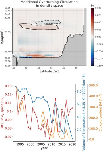
Zhang (Citation2010) argued that the variations in the MOC-density space are significantly different than those in the MOC-depth space especially close to the water formation regions. The Black Sea is very narrow in the north–south direction; thus, it would be important to study the evolution of the MOC-density space in the whole basin. (b) depicts the time evaluation of the maximum BS-MOC in density space between 22.45 and 23.85 kg m⁻³ (red line) together with the timeseries of the monthly model mean of volume of water masses below the temperature criteria (T < 8.35°C) where the bathymetry is deeper than 1000 m (blue line) and the CIL cold content computed using ship data and Argo floats (orange line) from Capet et al. Citation2020. The CIL cold content defined by the same temperature criteria above shows a significant reduction from 1993 to 2010 in the observations. The model captures this reduction well with a decrease of the volume of water mass in the deep basin. The maximum BS-MOC value has also decreased during this period from 0.13 to 0.07 Sv. After 2010, there were a couple of years of increasing of the CIL content accompanied with an increase in the maximum BS-MOC and volume of temperature fields. There was another peak in 2017 for the CIL cold content and maximum BS-MOC. Over the last 30 years, the Black Sea MOC has decreased indicating a climate shift possibly due to anthropogenic global warming (Stanev et al. Citation2019). The proposed maximum BS-MOC in density space can be potentially used as long-term climate monitoring index.

Finally, the temperature/salinity (T/S) diagram at a single grid point (43.5°N, 31°E) at the deep western basin of the Black Sea is shown in as a function of seven different periods (4 years averaged), together with climatology values obtained from SeaDataCloud dataset (product ref. 2.9.2). This open ocean location is away from coastal boundaries, CIL formation and MW injection sites. Thus, we can track the evolution of the background stratification in the Black Sea. The dashed red line represents the 8.35°C criterion of Capet et al. Citation2020 (product ref. 2.9.3) used to identify CIL waters. Four $σ_{2}$ values of 19.75, 22.45, 23.85 and 25.87 kg m⁻³ are also shown as black contours. The number of points below the critical temperature at each time interval are shown in the bottom left corner of each figure. In the first decade of the simulation, there were more 20,000 grid points below the critical temperature, then it reduces down to 15,594 between 2009 and 2012, 11,790 between 2013 and 2016, and finally down to 10,381 points between 2017 and 2020. Decrease (increase) of number points below (above) this line is a clear signal of the reduction of the CIL cold content (warming of the Black Sea mid-pycnocline). During the first 4 years of the simulation, the CIL cold content is higher as compared to the rest of the simulation period. In the second and third 4-years periods the CIL signal is weakening and is the lowest between 2009 and 2016. This is confirmed by observations as shown in for which at the increased temperature compromises the persistence of CIL which is correlated with the maximum BS-MOC evolution in density space (red line in ).

Figure 2.9.3. T–S diagrams from BS-REA for a 4-year period starting from 1993. Grey crosses show T–S climatological (1995–2020) data from SeaDataCloud (Myroshnychenko Citation2020, product ref. 2.9.2). Dashed line represents 8.35°C isothermal. The number of grid points below the 8.35 isothermal are shown in the bottom left corner of each figure.

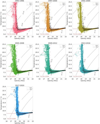
2.9.4. Conclusions

In this study, we analyzed for the first time the meridional overturning circulation in the Black Sea to describe the water mass properties, in particular the role of the vertical stratification which is strictly dependent on the Mediterranean inflow and the CIL. This analysis has been performed using an eddy-resolving reanalysis product for the Black Sea (Lima et al. Citation2021). Starting from a consolidated approach for the understanding of the global ocean overturning, recently applied also in the Mediterranean Sea, we computed the meridional overturning circulation for the Black Sea in both depth and density space. It revealed the presence of a clockwise circulation in the northern part up to 150 m connected to CIL cold content and an anticlockwise circulation in the southern part that could be connected to the influence of the Mediterranean Water inflow into the Black Sea.

The CIL has been represented by a cyclonic cell in the BS-MOC mean field. On the other hand, the Mediterranean Water from the Bosphorus Strait goes under the CIL and has an anticyclonic circulation. This counterclockwise cell might be considered as a ‘diffusive cell’. The MW mixes with ambient background waters due to double diffusion (Özsoy and Beșiktepe Citation1995). We do not find a statistically significant trend in the time evolution of the maximum value of the BS-MOC in depth space.

Next, we computed BS-MOC in density space. We propose a new index which is the maximum overturning circulation in density space between 22.45 and 23.85 kg m⁻³. This new index has a very strong correlation with the observed Cold Intermediate Layer cold content in the Black Sea (0.7 correlation coefficient with the Argo float data), and it can help us to monitor long-term climate variability in the Black Sea. We found that the BS-MOC has been weakened between 1993 and 2010 from 0.13 Sv down to 0.07 Sv, then it recovered and has equilibrated around 0.1 Sv. Time evolution of the BS-MOC values also overlap with warmer mixed layer temperature.

Next steps will focus on deepening the investigation of the role of the overturning circulation as a mechanism for understanding the Black Sea climate system and to supply oxygen in the upper 200–250 m of the basin. One of the limits of the current modelling approach is related to the implementation of the boundary conditions at the Bosphorus Strait: it is a closed boundary where the net outflow remains constant in time is governed by the imposition of a surface boundary condition able to balance the water budget at basin scale. Implementation of realistic lateral boundary conditions for the Mediterranean waters inflow into the Black Sea will be a future improvement in the reanalysis product. This could address significant findings in the general understanding of the overturning circulation in the Black Sea through a better representation of the interactions between the two marginal seas. Nevertheless, the role of rivers and atmospheric circulation at basin scale is considered a challenge to better understand the correlation between the BS-MOC and the CIL and for the monitoring of the climate properties of the basin. Another relevant recommendation is the link between observations and Black Sea MOC: enforcing the observing network for the overturning circulation as described for the AMOC in Frajka-Williams et al. Citation2019 could provide new insights for the monitoring of critical climate phenomena as well as extreme events in the Black Sea.

Supplemental material

Supplemental Material

Supplemental Material

References

Aboobacker VM, Shanas PR, Al-Ansari EMAS, Sanil Kumar V, Vethamony P. 2021. The maxima in northerly wind speeds and wave heights over the Arabian Sea, the Arabian/Persian Gulf and the Red Sea derived from 40 years of ERA5 data. Clim Dyn. 56:1037–1052. doi:10.1007/s00382-020-05518-6.
Web of Science ®Google Scholar
Belmonte Rivas M, Stoffelen A. 2019. Characterizing ERA-Interim and ERA5 surface wind biases using ASCAT. Ocean Sci. 15:831–852. doi:10.5194/os-15-831-2019.
Web of Science ®Google Scholar
Belmonte Rivas M, Stoffelen A, Bentamy A. 2019. Sea surface winds and Ekman pumping. In: Copernicus Marine Service Ocean state report, issue 3. J Oper Oceanogr. 12(Suppl. 1):S1–S123. doi:10.1080/1755876X.2019.1633075.
Google Scholar
Bevere L, Fan I, Holzheu T. 2020. Swiss Re Institute estimates USD 83 billion global insured catastrophe losses in 2020, the fifth-costliest on record, Swiss Re web article. [cited 27 Dec 2020]. https://www.swissre.com/media/news-releases/nr-20201215-sigma-full-year-2020-preliminary-natcat-loss-estimates.html.
Google Scholar
Bian G-F, Nie G-Z, Qiu X. 2021. How well is outer tropical cyclone size represented in the ERA5 reanalysis dataset? Atmos Res. 249:105339. doi:10.1016/j.atmosres.2020.105339.
Web of Science ®Google Scholar
Bourassa MA, Meissner T, Cerovecki I, Chang PS, Dong X, De Chiara G, Donlon C, Dukhovskoy DS, Elya J, Fore A, et al. 2019. Remotely sensed winds and wind stresses for marine forecasting and ocean modeling. Front Mar Sci. 6:443. doi:10.3389/fmars.2019.00443.
Web of Science ®Google Scholar
Collins M, Sutherland M, Bouwer L, Cheong S-M, Frölicher T, Jacot Des Combes H, Koll Roxy M, Losada I, McInnes K, Ratter B, et al. 2019. Extremes, abrupt changes and managing risk. In: IPCC special report on the ocean and cryosphere in a changing climate [H-O. Pörtner, DC Roberts, V Masson-Delmotte, P Zhai, M Tignor, E Poloczanska, K Mintenbeck, A Alegría, M Nicolai, A Okem, J Petzold, B Rama, NM Weyer, editors]. In press.
Google Scholar
Davies PA, McCarthy M, Christidis N, Dunstone N, Fereday D, Kendon M, Knight JR, Scaife AA, Sexton D. 2021. The wet and stormy UK winter of 2019/2020. Weather. doi:10.1002/wea.3955.
PubMed Web of Science ®Google Scholar
de Kloe J, Stoffelen A, Verhoef A. 2017. Improved use of scatterometer measurements by using stress-equivalent reference winds. IEEE J. Sel. Top. Appl. Earth Obs. Remote Sens. 10:2340–2347. doi:10.1109/JSTARS.2017.2685242.
Web of Science ®Google Scholar
Dong B, Sutton RT, Woollings T, Hodges K. 2013. Variability of the North Atlantic summer storm track: mechanisms and impacts on European climate. Environ Res Lett. 8:034037. doi:10.1088/1748-9326/8/3/034037.
Web of Science ®Google Scholar
Dullaart JCM, Muis S, Bloemendaal N, Aerts JCJH. 2020. Advancing global storm surge modelling using the new ERA5 climate reanalysis. Clim Dyn. 54:1007–1021. doi:10.1007/s00382-019-05044-0.
Web of Science ®Google Scholar
Earl N, Dorling S, Hewston R, von Glasow R. 2013. 1980–2010 variability in U.K. surface wind climate. J Clim. 26(4):1172–1191. doi:10.1175/JCLI-D-12-00026.1.
Web of Science ®Google Scholar
Hoskins BJ, Hodges KI. 2005. A new perspective on Southern hemisphere storm tracks. J Clim. 18(20):4108–4129. doi:10.1175/JCLI3570.1.
Web of Science ®Google Scholar
Hu S, Hu D, Guan C, Xing N, Li J, Feng J. 2017. Variability of the western Pacific warm pool structure associated with El Niño. Clim Dyn. 49:2431–2449. doi:10.1007/s00382-016-3459-y.
Web of Science ®Google Scholar
IPCC. 2021. Climate change 2021: the physical science basis. Contribution of working group I to the sixth assessment report of the intergovernmental panel on climate change [V Masson-Delmotte, P Zhai, A Pirani, SL Connors, C Péan, S Berger, N Caud, Y Chen, L Goldfarb, MI Gomis, M Huang, K Leitzell, E Lonnoy, JBR Matthews, TK Maycock, T Waterfield, O Yelekçi, R Yu, B Zhou, editors]. Cambridge University Press. In press.
Google Scholar
Knutson T, Camargo SJ, Chan JCL, Emanuel K, Ho C, Kossin J, Mohapatra M, Satoh M, Sugi M, Walsh K, Wu L. 2020. Tropical cyclones and climate change assessment: part II: projected response to anthropogenic warming. Bull Am Meteorol Soc. 101(3):E303–E322. doi:10.1175/BAMS-D-18-0194.1.
Web of Science ®Google Scholar
Laurila TK, Sinclair VA, Gregow H. 2021. Climatology, variability, and trends in near-surface wind speeds over the North Atlantic and Europe during 1979–2018 based on ERA5. Int J Climatol. 41:2253–2278. doi:10.1002/joc.6957.
Web of Science ®Google Scholar
Lee S-S, Lee J-Y, Wang B, Ha K-J, Heo K-Y, Jin F-F, Straus DM, Shukla J. 2012. Interdecadal changes in the storm track activity over the North Pacific and North Atlantic. Clim Dyn. 39:313–327. doi:10.1007/s00382-011-1188-9.
Web of Science ®Google Scholar
Marseille G-J, Stoffelen A, van den Brink H, Stepek A. 2019. WISC bias derivation and uncertainty assessment, C3S windstorm information service – copernicus (WISC), Doc. C3S_441_Lot3_WISC_SC2-D3.3-CGI-RP-17-0071, KNMI. Available from: https://wisc.climate.copernicus.eu/wisc/documents/shared/(C3S_441_Lot3_WISC_SC2-D3.3-CGI-RP-17-0071)%20(Final%20Bias%20Derivation)%20(v1.0).pdf.
Google Scholar
Moore GWK, Renfrew IA. 2005. Tip jets and barrier winds: a QuikSCAT climatology of high wind speed events around Greenland. J Clim. 18(18):3713–3725. doi:10.1175/JCLI3455.1.
Web of Science ®Google Scholar
Oliver EC, Lago V, Hobday AJ, Holbrook NJ, Ling SD, Mundy CN. 2018. Marine heatwaves off eastern Tasmania: trends, interannual variability, and predictability. Prog Oceanogr. 161:116–130.
Web of Science ®Google Scholar
Russell JL, Long DG, Chang PS, Cowell M, Curchitser E, Dinniman MS, Fellows C, Goodman PJ, Hofmann EE, Jelenak Z, et al. 2021. Measuring vector winds from space to reduce the uncertainty in the Southern Ocean carbon fluxes: science requirements and proposed mission. Geophys Res Lett, in review.
Google Scholar
Sampe T, Xie S. 2007. Mapping high sea winds from space: a global climatology. Bull. Am. Meteorol. Soc. 88:1965-1978. doi:10.1175/BAMS-88-12-1965.
Web of Science ®Google Scholar
Schreck CJS, Knapp KR, Kossin JP. 2014. The impact of best track discrepancies on global tropical cyclone climatologies using IBTrACS. Mon Weather Rev. 142(10):3881–3899. doi:10.1175/MWR-D-14-00021.1.
Web of Science ®Google Scholar
Shaw TA, Baldwin M, Barnes EA, Caballero R, Garfinkel CI, Hwang Y-T, Li C, O’Gorman PA, Rivière G, Simpson IR, Voigt A. 2016. Storm track processes and the opposing influences of climate change. Nat Geosci. 9:656–664. doi:10.1038/ngeo2783.
Web of Science ®Google Scholar
Stoffelen A, Mouche A, Polverari F, van Zadelhoff G-J, Sapp J, Portabella M, Chang P, Lin W, Jelenak Z. 2020. C-band high and extreme-force speeds (CHEFS) – final report, EUMETSAT project report, KNMI. Available from: https://www-cdn.eumetsat.int/files/2020-06/pdf_ss_chefs_final_rep.pdf.
Google Scholar
Tilburg CE, Hurlburt HE, O'Brien JJ, Shriver JF. 2001. The dynamics of the East Australian current system: the Tasman front, the East Auckland current, and the East Cape current. J Phys Oceanogr. 31(10):2917–2943.
Web of Science ®Google Scholar
Wang C, Wu K, Wu L, Zhao H, Cao J. 2021. What caused the unprecedented absence of western North Pacific tropical cyclones in July 2020? Geophys Res Lett. 48:e2020GL092282. doi:10.1029/2020GL092282.
Web of Science ®Google Scholar
Wang Z, Stoffelen A, Zhang B, He Y, Lin W, Li X. 2019. Inconsistencies in scatterometer wind products based on ASCAT and OSCAT-2 collocations. Remote Sens Environ. 225:207–216. doi:10.1016/j.rse.2019.03.005.
Web of Science ®Google Scholar
Yeasmin A, Chand S, Turville C, Sultanova N. 2021. Detection and verification of tropical cyclones and depressions over the South Pacific Ocean basin using ERA-5 reanalysis dataset. Int J Climatol. 41:5318–5330. doi:10.1002/joc.7131.
Web of Science ®Google Scholar
Young IR, Ribal A. 2019. Multiplatform evaluation of global trends in wind speed and wave height. Science. 364:548–552. doi:10.1126/science.aav9527.
PubMed Web of Science ®Google Scholar
Buckley MW, Marshall J. 2016. Observations, inferences, and mechanisms of the Atlantic Meridional Overturning Circulation: a review. Rev Geophys. 54(1):5–63. doi:10.1002/2015RG000493.
Web of Science ®Google Scholar
Caesar L, Rahmstorf S, Robinson A, Feulner G, Saba V. 2018. Observed fingerprint of a weakening Atlantic Ocean Overturning Circulation. Nature. 556(7700):191–196. doi:10.1038/s41586-018-0006-5.
PubMed Web of Science ®Google Scholar
Collins M, Sutherland M, Bouwer L, Cheong S-M, Frölicher T, Jacot Des Combes H, Koll Roxy M, Losada I, McInnes K, Ratter B, et al. 2019. Extremes, abrupt changes and managing risk, in H-O Pörtner; DC Roberts; V Masson-Delmotte; P Zhai; M Tignor; E Poloczanska; K Mintenbeck; A Alegría; M Nicolai; A Okem; J Petzold; B Rama, NM Weyer, editors. IPCC special report on the ocean and cryosphere in a changing climate.
Google Scholar
Danabasoglu G, Yeager SG, Kim WM, Behrens E, Bentsen M, Bi D, Biastoch A, Bleck R, Böning C, Bozec A, et al. 2016. North Atlantic simulations in coordinated Ocean-ice reference experiments phase II (CORE-II). Part II: inter-annual to decadal variability. Ocean Modell. 97:65–90. doi:10.1016/j.ocemod.2015.11.007.
Web of Science ®Google Scholar
Dee DP, Uppala SM, Simmons AJ, Berrisford P, Poli P, Kobayashi S, Andrae U, Balmaseda MA, Balsamo G, Bauer P, et al. 2011. The ERA-Interim reanalysis: configuration and performance of the data assimilation system. Q J R Metereol Soc. 137(656):553–597. doi:10.1002/qj.828.
Web of Science ®Google Scholar
Desbruyères DG, Mercier H, Maze G, Daniault N. 2019. Surface predictor of overturning circulation and heat content change in the subpolar North Atlantic. Ocean Sci. 15(3):809–817. doi:10.5194/os-15-809-2019.
Web of Science ®Google Scholar
Fu Y, Li F, Karstensen J, Wang C. 2020. A stable Atlantic Meridional Overturning Circulation in a changing North Atlantic Ocean since the 1990s. Sci Adv. 6(48):eabc7836. doi:10.1126/sciadv.abc7836.
PubMed Web of Science ®Google Scholar
Jackson LC, Dubois C, Forget G, Haines K, Harrison M, Iovino D, Köhl A, Mignac D, Masina S, Peterson KA, et al. 2019. The mean state and variability of the North Atlantic circulation: a perspective from ocean reanalyses. J Geophys Res Oceans. 124(12):9141–9170. doi:10.1029/2019JC015210.
Web of Science ®Google Scholar
Jackson L, Dubois C, Masina S, Storto A, Zuo H. 2018. Atlantic Meridional Overturning Circulation. In: von Schuckmann et al. the Copernicus Marine Service Ocean state report. J Operat Ocean. 11(Suppl. 1):S1–S142.
Google Scholar
Jackson LC, Peterson KA, Roberts CD, Wood RA. 2016. Recent slowing of Atlantic overturning circulation as a recovery from earlier strengthening. Nat Geosci. 9(7):518–522. doi:10.1038/ngeo2715.
Web of Science ®Google Scholar
Lellouche JM, Le Galloudec O, Drévillon M, Régnier C, Greiner E, Garric G, Ferry N, Desportes C, Testut CE, Bricaud C, et al. 2013. Evaluation of global monitoring and forecasting systems at Mercator Océan. Ocean Sci. 9(1):57–81. doi:10.5194/os-9-57-2013.
Web of Science ®Google Scholar
Li F, Lozier MS, Bacon S, Bower AS, Cunningham SA, de Jong MF, deYoung B, Fraser N, Fried N, Han G, et al. 2021. Subpolar North Atlantic western boundary density anomalies and the meridional overturning circulation. Nat Commun. 12(1):3002. doi:10.1038/s41467-021-23350-2.
PubMed Web of Science ®Google Scholar
Li F, Lozier MS, Johns WE. 2017. Calculating the meridional volume, heat, and freshwater transports from an observing system in the subpolar North Atlantic: observing system simulation experiment. J Atmos Ocean Technol. 34(7):1483–1500. doi:10.1175/JTECH-D-16-0247.1.
Web of Science ®Google Scholar
Lozier MS, Bacon S, Bower AS, Cunningham SA, De Jong MF, De Steur L, De Young B, Fischer J, Gary SF, Greenan BJW, et al. 2017. Overturning in the subpolar north Atlantic program: a new international ocean observing system. Bull Am Meteorol Soc. 98(4):737–752. doi:10.1175/BAMS-D-16-0057.1.
Web of Science ®Google Scholar
Lozier MS, Li F, Bacon S, Bahr F, Bower AS, Cunningham SA, De Jong MF, De Steur L, DeYoung B, Fischer J, et al. 2019. A sea change in our view of overturning in the subpolar North Atlantic. Science. 363(6426):516–521. doi:10.1126/science.aau6592.
PubMed Web of Science ®Google Scholar
MacLachlan C, Arribas A, Peterson KA, Maidens A, Fereday D, Scaife AA, Gordon M, Vellinga M, Williams A, Comer RE, et al. 2015. Global seasonal forecast system version 5 (GloSea5): a high-resolution seasonal forecast system. Q J R Metereol Soc. 141(689):1072–1084. doi:10.1002/qj.2396.
Web of Science ®Google Scholar
Menary MB, Jackson LC, Lozier MS. 2020. Reconciling the relationship between the AMOC and Labrador Sea in OSNAP observations and climate models. Geophys Res Lett. 47(18):e2020GL089793. doi:10.1029/2020GL089793.
Web of Science ®Google Scholar
Moffa-Sánchez P, Moreno-Chamarro E, Reynolds DJ, Ortega P, Cunningham L, Swingedouw D, Amrhein DE, Halfar J, Jonkers L, Jungclaus JH, et al. 2019. Variability in the Northern North Atlantic and Arctic Oceans across the last two millennia: a review. Paleoceanogr Paleoclimatol. 34(8):1399–1436. doi:10.1029/2018PA003508.
Web of Science ®Google Scholar
Rahmstorf S. 2015. Exceptional twentieth-century slowdown in Atlantic Ocean overturning circulation. Nat Clim Chang. 5(5):475–480. doi:10.1038/nclimate2554.
Web of Science ®Google Scholar
Robson J, Lohmann K, Smith D, Palmer MD. 2012. Causes of the rapid warming of the North Atlantic Ocean in the mid-1990s. J Clim. 25(12):4116–4134. doi:10.1175/JCLI-D-11-00443.1.
Web of Science ®Google Scholar
Srokosz M, Baringer M, Bryden H, Cunningham S, Delworth T, Lozier S, Marotzke J, Sutton R. 2012. Past, present, and future changes in the Atlantic Meridional Overturning Circulation. Bull Am Meteorol Soc. 93(11):1663–1676. doi:10.1175/BAMS-D-11-00151.1.
Web of Science ®Google Scholar
Storto A, Masina S, Navarra A. 2016. Evaluation of the CMCC eddy-permitting global ocean physical reanalysis system (C-GLORS, 1982–2012) and its assimilation components. Q J R Metereol Soc. 142(695):738–758. doi:10.1002/qj.2673.
Web of Science ®Google Scholar
Thornalley DJR, Oppo DW, Ortega P, Robson JI, Brierley CM, Davis R, Hall IR, Moffa-Sanchez P, Rose NL, Spooner PT, et al. 2018. Anomalously weak Labrador Sea convection and Atlantic overturning during the past 150 years. Nature. 556(7700):227–230. doi:10.1038/s41586-018-0007-4.
PubMed Web of Science ®Google Scholar
von Schuckmann K, Le Traon PY, Smith N, Pascual A, Brasseur P, Fennel K, Djavidnia S, Aaboe S, Fanjul EA, Autret E, et al. 2018. Copernicus Marine Service Ocean state report. J Oper Oceanogr. 11(Suppl. 1):S1–S142. doi:10.1080/1755876X.2018.1489208.
Google Scholar
Zuo H, Balmaseda MA, Tietsche S, Mogensen K, Mayer M. 2019. The ECMWF operational ensemble reanalysis-analysis system for ocean and sea ice: a description of the system and assessment. Ocean Sci. 15(3):779–808. doi:10.5194/os-15-779-2019.
Web of Science ®Google Scholar
Zuo H, Balmaseda MA, de Boisseson E, Tietsche S, Mayer M, de Rosnay P. 2021. The ORAP6 ocean and sea-ice reanalysis: description and evaluation. EGU General Assembly 2021. EGU21-9997. https://doi.org/10.5194/egusphere-egu21-9997.
Google Scholar
Zou S, Lozier MS, Li F, Abernathey R, Jackson L. 2020. Density-compensated overturning in the Labrador Sea. Nat Geosci. 13(2):121–126. doi:10.1038/s41561-019-0517-1.
Web of Science ®Google Scholar
Årthun M, Eldevik T. 2016. On anomalous ocean heat transport toward the Arctic and associated climate predictability. J Clim. 29(2):689–704.
Web of Science ®Google Scholar
Asbjørnsen H, Årthun M, Skagseth Ø, Eldevik T. 2019. Mechanisms of ocean heat anomalies in the Norwegian Sea. J Geophys Res Oceans. 124(4):2908–2923.
Web of Science ®Google Scholar
Asbjørnsen H, Johnson HL, Årthun M. 2021. Variable Nordic Seas inflow linked to shifts in North Atlantic circulation. J Clim. 34(17):7057–7071.
Web of Science ®Google Scholar
Berx B, et al. 2013. Combining in situ measurements and altimetry to estimate volume, heat and salt transport variability through the faroe–Shetland channel. Ocean Sci. 9:639–654.
Web of Science ®Google Scholar
Bosse A, Fer I, Søiland H, Rossby T. 2018. Atlantic water transformation along its poleward pathway across the Nordic Seas. J Geophys Res Oceans. 123(9):6428–6448.
Web of Science ®Google Scholar
Bringedal C, Eldevik T, Skagseth Ø, Spall MA, Østerhus S. 2018. Structure and forcing of observed exchanges across the Greenland–Scotland ridge. J Clim. 31(24):9881–9901.
Web of Science ®Google Scholar
Buckley MW, Marshall J. 2016. Observations, inferences, and mechanisms of the Atlantic Meridional Overturning Circulation: a review. Rev Geophys. 54(1):5–63.
Web of Science ®Google Scholar
Chafik L, Rossby T. 2019. Volume, heat, and freshwater divergences in the subpolar North Atlantic suggest the Nordic Seas as key to the state of the meridional overturning circulation. Geophys Res Lett. 46(9):4799–4808.
Web of Science ®Google Scholar
Curry JA, Schramm JL, Ebert EE. 1995. Sea ice-albedo climate feedback mechanism. J Clim. 8(2):240–247.
Web of Science ®Google Scholar
Hansen B, Østerhus S, Turrell WR, Jónsson S, Valdimarsson H, Hátún H, Olsen SM. 2008. The inflow of Atlantic water, heat, and salt to the Nordic seas across the Greenland–Scotland ridge. In: Arctic–Subarctic ocean fluxes. Dordrecht: Springer; p. 15–43.
Google Scholar
Hersbach H, Bell B, Berrisford P, Hirahara S, Horányi A, Muñoz-Sabater J, Nicolas J, Peubey C, Radu R, Schepers D, et al. 2020. The ERA5 global reanalysis. Q J R Metereol Soc. 146(730):1999–2049.
Web of Science ®Google Scholar
Jackson LC, Kahana R, Graham T, Ringer MA, Woollings T, Mecking JV, Wood RA. 2015. Global and European climate impacts of a slowdown of the AMOC in a high resolution GCM. Clim Dyn. 45(11):3299–3316.
Web of Science ®Google Scholar
Jónsson S, Valdimarsson H. 2012. Water mass transport variability to the North Icelandic shelf, 1994–2010. ICES J Mar Sci. 69:809–815.
Web of Science ®Google Scholar
Hansen B, Larsen KMH, Hátún H, Kristiansen R, Mortensen E, Østerhus S. 2015. Transport of volume, heat, and salt towards the Arctic in the Faroe Current 1993–2013. Ocean Sci. 11:743–757.
Web of Science ®Google Scholar
Hansen B, Østerhus S. 2000. North Atlantic-Nordic Seas exchanges. Prog Oceanogr. 45:109–208.
Web of Science ®Google Scholar
Hátún H, Sandø AB, Drange H, Hansen B, Valdimarsson H. 2005. Influence of the Atlantic subpolar gyre on the thermohaline circulation. Science. 309(5742):1841–1844.
PubMed Web of Science ®Google Scholar
Kobayashi S, Ota Y, Harada Y, Ebita A, Moriya M, Onoda H, Onogi K, Kamahori H, Kobayashi C, Endo H, Miyaoka, K, et al. 2015. The JRA-55 reanalysis: general specifications and basic characteristics. J Meteorol Soc Jpn Ser II. 93(1):5–48.
Web of Science ®Google Scholar
Loeb NG, Doelling DR, Wang H, Su W, Nguyen C, Corbett JG, Liang L, Mitrescu C, Rose FG, Kato S. 2018. Clouds and the earth’s radiant energy system (CERES) energy balanced and filled (EBAF) top-of-atmosphere (TOA) edition-4.0 data product. J Clim. 31(2):895–918.
Web of Science ®Google Scholar
Mauritzen C. 1996. Production of dense overflow waters feeding the North Atlantic across the Greenland-Scotland ridge. Part 1: evidence for a revised circulation scheme. Deep Sea Res Part I. 43(6):769–806.
Web of Science ®Google Scholar
Mayer J, Mayer M, Haimberger L. 2021. Consistency and homogeneity of atmospheric energy, moisture, and mass budgets in ERA5. J Clim. 34(10):3955–3974.
Web of Science ®Google Scholar
Mayer M, Haimberger L, Pietschnig M, Storto A. 2016. Facets of Arctic energy accumulation based on observations and reanalyses 2000–2015. Geophys Res Lett. 43(19):10–420.
Web of Science ®Google Scholar
Mayer M, Haimberger L, Edwards JM, Hyder P. 2017. Toward consistent diagnostics of the coupled atmosphere and ocean energy budgets. J Clim. 30(22):9225–9246.
Web of Science ®Google Scholar
Mayer M, Lien VS, Mork KA, von Schuckmann K, Monier M, Greiner E. 2021. Ocean heat content in the High North. In CMEMS ocean state report vol. 5, accepted in Journal of Operational Oceanography.
Google Scholar
Mayer M, Tietsche S, Haimberger L, Tsubouchi T, Mayer J, Zuo H. 2019. An improved estimate of the coupled Arctic energy budget. J Clim. 32(22):7915–7934.
Web of Science ®Google Scholar
Muilwijk M, Smedsrud LH, Ilicak M, Drange H. 2018. Atlantic Water heat transport variability in the 20th century Arctic Ocean from a global ocean model and observations. J Geophys Res Oceans. 123(11):8159–8179.
Web of Science ®Google Scholar
Oort AH, Yienger JJ. 1996. Observed interannual variability in the Hadley circulation and its connection to ENSO. J Clim. 9(11):2751–2767.
Web of Science ®Google Scholar
Østerhus S, Woodgate R, Valdimarsson H, Turrell B, de Steur L, Quadfasel D, Olsen SM, Moritz M, Lee CM, Larsen KMH, et al. 2019. Arctic Mediterranean exchanges: a consistent volume budget and trends in transports from two decades of observations. Ocean Sci. 15:379–399.
Web of Science ®Google Scholar
Polyakov IV, Pnyushkov AV, Alkire MB, Ashik IM, Baumann TM, Carmack EC, Goszczko I, Guthrie J, Ivanov VV, Kanzow T, et al. 2017. Greater role for Atlantic inflows on sea-ice loss in the Eurasian Basin of the Arctic Ocean. Science. 356(6335):285–291.
PubMed Web of Science ®Google Scholar
Richter K, Segtnan OH, Furevik T. 2012. Variability of the Atlantic inflow to the Nordic Seas and its causes inferred from observations of sea surface height. J Geophys Res. 117:C04004. doi:10.1029/2011JC007719.
Web of Science ®Google Scholar
Rudels B, Marnela M, Eriksson P. 2008. Constraints on estimating mass, heat and freshwater transports in the Arctic Ocean: an exercise. In: Robert R. Dickson, Jens Meincke, Peter Rhines, editors. Arctic–Subarctic ocean fluxes. Dordrecht: Springer; p. 315–341.
Google Scholar
Shu Q, Wang Q, Song Z, Qiao F. 2021. The poleward enhanced Arctic Ocean cooling machine in a warming climate. Nat Commun. 12(1):1–9.
PubMed Web of Science ®Google Scholar
Skagseth Ø, Eldevik T, Årthun M, Asbjørnsen H, Lien VS, Smedsrud LH. 2020. Reduced efficiency of the Barents Sea cooling machine. Nat Clim Change. doi:10.1038/s41558-020-0772-6.
Web of Science ®Google Scholar
Swift JH, Aagaard K. 1981. Seasonal transitions and water mass formation in the Iceland and Greenland Seas. Deep Sea Res A. 28(10). doi:10.1016/0198-0149(81)90050-9.
Web of Science ®Google Scholar
Trenberth KE, Fasullo JT. 2017. Atlantic meridional heat transports computed from balancing Earth’s energy locally. Geophys Res Lett. 44(4):1919–1927.
Web of Science ®Google Scholar
Tsubouchi T, Bacon S, Aksenov Y, Garabato ACN, Beszczynska-Möller A, Hansen E, de Steur L, Curry B, Leeet CM. 2018. The Arctic Ocean seasonal cycles of heat and freshwater fluxes: observation-based inverse estimates. J Phys Oceanogr. 48(9):2029–2055.
Web of Science ®Google Scholar
Tsubouchi T, Våge K, Hansen B, Larsen KMH, Østerhus S, Johnson C, Jónsson S, Valdimarsson H. 2021. Increased ocean heat transport into the Nordic Seas and Arctic Ocean over the period 1993–2016. Nat Clim Change. 11(1):21–26.
Web of Science ®Google Scholar
Von Schuckmann K, Palmer MD, Trenberth KE, Cazenave A, Chambers D, Champollion N, Hansen J, Josey SA, Loeb N, Mathieu P-P, et al. 2016. An imperative to monitor Earth's energy imbalance. Nat Clim Change. 6(2):138–144.
Web of Science ®Google Scholar
Williams RG, Roussenov V, Lozier MS, Smith D. 2015. Mechanisms of heat content and thermocline change in the subtropical and subpolar North Atlantic. J Clim. 28(24):9803–9815. [cited 2021 Nov 12]. Available from: https://journals.ametsoc.org/view/journals/clim/28/24/jcli-d-15-0097.1.xml.
Web of Science ®Google Scholar
Zuo H, Balmaseda MA, Tietsche S, Mogensen K, Mayer M. 2019. The ECMWF operational ensemble reanalysis–analysis system for ocean and sea ice: a description of the system and assessment. Ocean science. 15(3):779–808.
Web of Science ®Google Scholar
Barber DG, Hop H, Mundy CJ, Else B, Dmitrenko IA, Tremblay JE, Ehn JK, Assmy P, Daase M, Candlish LM, Rysgaard S. 2015. Selected physical, biological and biogeochemical implications of a rapidly changing Arctic Marginal Ice Zone. Prog. Oceanogr. 139:122-150. doi:10.1016/J.Pocean.2015.09.003.
Web of Science ®Google Scholar
Blanchard-Wrigglesworth E, Roach LA, Donohoe A, Ding Q. 2021. Impact of winds and Southern Ocean SSTs on Antarctic sea ice trends and variability. J Clim. 34:949–965. doi:10.1175/JCLI-D-20-0386.1.
Web of Science ®Google Scholar
Bintanja R, van Oldenborgh GJ, Drijfhout SS, Wouters B, Katsman CA. 2013. Important role for ocean warming and increased ice-shelf melt in Antarctic sea-ice expansion. Nat Geosci. 6:376–379. doi:10.1038/ngeo1767.
Web of Science ®Google Scholar
Comiso JC, Gersten RA, Stock LV, Turner J, Perez GJ, Cho K. 2017. Positive trend in the Antarctic sea ice cover and associated changes in surface temperature. J Clim. 30(6):2251–2267. doi:10.1175/JCLI-D-16-0408.1.
Web of Science ®Google Scholar
Dee DP, Uppala SM, Simmons AJ, Berrisford P, Poli P, Kobayashi S, Andrae U, Balmaseda MA, Balsamo G, Bauer P, et al. 2011. The ERA-Interim reanalysis: configuration and performance of the data assimilation system. Quart J Royal Meteorol Soc. 137(656):553–597. doi:10.1002/qj.828.
Web of Science ®Google Scholar
Dumont D, Kohout A, Bertino L. 2011. A wave-based model for the marginal ice zone including a floe breaking parameterization. J Geophys Res Ocean. 116:C04001. doi:10.1029/2010JC006682.
Web of Science ®Google Scholar
Eayrs C, Li X, Raphael MN, Holland DM. 2021. Rapid decline in Antarctic sea ice in recent years hints at future change. Nature Geosci. 14:460–464. doi:10.1038/s41561-021-00768-3.
Web of Science ®Google Scholar
Goosse H, Zunz V. 2014. Decadal trends in the Antarctic sea ice extent ultimately controlled by ice-ocean feedback. Cryosphere. 8:453–470. doi:10.5194/tc-8-453-2014.
Web of Science ®Google Scholar
Haid V, Iovino D, Masina S. 2017. Impacts of freshwater changes on Antarctic sea ice in an eddy-permitting sea-ice–ocean model. Cryosphere. 11:1387–1402. doi:10.5194/tc-11-1387-2017.
Web of Science ®Google Scholar
Hobbs WR, Massom R, Stammerjohn S, Reid P, Williams G, Meier W. 2016. A review of recent changes in Southern ocean sea ice, their drivers and forcings. Glob Planet Change. 143:228–250. doi:10.1016/j.gloplacha.2016.06.008.
Web of Science ®Google Scholar
Holland PR, Kwok R. 2012. Wind-driven trends in Antarctic sea-ice drift. Nat Geosci. 5:872–875. doi:10.1038/ngeo1627.
Web of Science ®Google Scholar
Holland PR, Bruneau N, Enright C, Losch M, Kurtz NT, Kwok R. 2014. Modeled trends in Antarctic sea ice thickness. J Clim. 27:3784–3801. doi:10.1175/JCLI-D-13-00301.1.
Web of Science ®Google Scholar
Ivanova N, Pedersen LT, Tonboe RT, Kern S, Heygster G, Lavergne T, Sørensen A, Saldo R, Dybkjær G, Brucker L, Shokr M. 2015. Inter-comparison and evaluation of sea ice algorithms: towards further identification of challenges and optimal approach using passive microwave observations. Cryosphere. 9:1797–1817. doi:10.5194/tc-9-1797-2015.
Web of Science ®Google Scholar
Lellouche JM, Le Galloudec O, Drevillon M, Regnier C, Greiner E, Garric G, Ferry N, Desportes C, Testut C-E, Bricaud C, et al. 2013. Evaluation of global monitoring and forecasting systems at Mercator Océan. Ocean Sci. 9(1):57–81. doi:10.5194/os-9-57-2013.
Web of Science ®Google Scholar
MacLachlan C, Arribas A, Peterson KA, Maidens A, Fereday D, Scaife AA, Gordon M, Vellinga M, Williams A, Comer RE, et al. 2015. Global Seasonal forecast system version 5 (GloSea5): a high-resolution seasonal forecast system. Quart J Royal Meteorol Soc. 141(689):1072–1084. doi:10.1002/qj.2396.
Web of Science ®Google Scholar
Maksym T. 2019. Arctic and Antarctic sea ice change: contrasts, commonalities, and causes. Ann Rev Mar Sci. 11:187–213. doi:10.1146/annurev-marine-010816-060610.
PubMed Web of Science ®Google Scholar
Maksym TE, Stammerjohn E, Ackley S, Massom R. 2012. Antarctic sea ice – a polar opposite? I. 25:140–151. doi:10.5670/oceanog.2012.88.
Google Scholar
Meehl GA, Arblaster JM, Bitz CM, Chung CTYY, Teng H. 2016. Antarctic sea-ice expansion between 2000 and 2014 driven by tropical Pacific decadal climate variability. Nature Geosci. 9:590–595. doi:10.1038/ngeo2751.
Web of Science ®Google Scholar
Meier WN, Fetterer F, Savoie M, Mallory S, Duerr R, Stroeve J. 2017. NOAA/NSIDC climate data record of passive microwave sea ice concentration, version 3. Boulder (CO): NSIDC: National Snow and Ice Data Center. https://nsidc.org/data/g02202/versions/3.
Google Scholar
Meier WN, Stewart JS. 2019. Assessing uncertainties in sea ice extent climate indicators. Environ Res Lett. 14:035005. doi:10.1088/1748-9326/aaf52c.
Web of Science ®Google Scholar
Meylan MH, Bennetts LG, Kohout AL. 2014. In situ measurements and analysis of ocean waves in the Antarctic marginal ice zone. Geophys Res Lett. 2(41):5046–5051. doi:10.1002/2014GL060809.
Google Scholar
Parkinson CL. 2019. A 40-y record reveals gradual Antarctic sea ice increases followed by decreases at rates far exceeding the rates seen in the Arctic. Proc Natl Acad Sci USA. 116:414–423. doi:10.1073/pnas.1906556116.
Web of Science ®Google Scholar
Paul F, Mielke T, Nisters C, Schröder J, Rampai T, Skatulla S, Audh R, Hepworth E, Vichi M, Lupascu DC. 2021. Brief communication: grease ice in the Antarctic marginal ice zone. Cryosphere Discuss. doi:10.5194/tc-2020-362.
Google Scholar
Pauling AG, Bitz CM, Smith IJ, Langhorne PJ. 2016. The response of the Southern Ocean and Antarctic sea ice to fresh water from ice shelves in an earth system model. J Climate. 29:1655–1672. doi:10.1175/JCLI-D-15-0501.1.
Web of Science ®Google Scholar
Peng G, Meier WN, Scott DJ, Savoie MH. 2013. A long-term and reproducible passive microwave sea ice concentration data record for climate studies and monitoring. Earth Syst Sci Data. 5:311–318. doi:10.5194/essd-5-311-2013.
Web of Science ®Google Scholar
Simmonds I. 2015. Comparing and contrasting the behaviour of Arctic and Antarctic sea ice over the 35-year period 1979–2013. Ann Glaciol. 56:18–28. doi:10.3189/2015AoG69A909.
Web of Science ®Google Scholar
Squire VA. 2007. Of ocean waves and sea-ice revisited. Cold Reg Sci Technol. 49:110–133. doi:10.1016/j.coldregions.2020.103042.
Web of Science ®Google Scholar
Storto A, Masina S, Simoncelli S, Iovino D, Cipollone A, Drevillon M, Drillet Y, von Schuckman K, Parent L, Garric G, et al. 2019. The added value of the multi-system spread information for ocean heat content and steric sea level investigations in the CMEMS GREP ensemble reanalysis product. Clim Dyn. 53:287–312. doi:10.1007/s00382-018-4585-5.
Web of Science ®Google Scholar
Stroeve JC, Jenouvrier S, Campbell GG, Barbraud C, Delord K. 2016. Mapping and assessing variability in the Antarctic marginal ice zone, pack ice and coastal polynyas in two sea ice algorithms with implications on breeding success of snow petrels. Cryosphere. 10:1823–1843. doi:10.5194/tc-10-1823-2016.
Web of Science ®Google Scholar
Sutherland BR, Balmforth NJ. 2019. Damping of surface waves by floating particles. Phys Rev Fluids. 4:014804. doi:10.1103/PhysRevFluids.4.014804.
Web of Science ®Google Scholar
Tonboe RT, Eastwood S, Lavergne T, Sørensen AM, Rathmann N, Dybkjær G, Pedersen LT, Høyer JL, Kern S. 2016. The EUMETSAT sea ice concentration climate data record. Cryosphere. 10:2275–2290. doi:10.5194/tc-10-2275-2016.
Web of Science ®Google Scholar
Venables HJ, Meredith MP. 2014. Feedbacks between ice cover, ocean stratifcation, and heat content in Ryder Bay, Western Antarctic Peninsula. J Geophys Res Oceans. 119:5323–5336. doi:10.1002/2013JC009669.
Web of Science ®Google Scholar
Vichi M. 2021. A statistical definition of the Antarctic marginal ice zone. Cryosphere. Discuss, in review. doi:10.5194/tc-2021-307
Google Scholar
Vichi M, Eayrs C, Alberello A, Bekker A, Bennetts L, Holland D, Jong E, Joubert W, MacHutchon K, Messori G, et al. 2019. Effects of an explosive polar cyclone crossing the Antarctic marginal ice zone. Geophys Res Lett. 46:5948–5958. doi:10.1029/2019GL082457.
Web of Science ®Google Scholar
Wadhams P. 2000. Ice in the Ocean. Amsterdam: Gordon and Breach Science Publishers, xii 351 p, illustrated, hard cover. ISBN 90-5699-296-1. £44.00; US$67.00. Polar Record, 38(206):269-270. doi:10.1017/S0032247400017848.
Google Scholar
Wadhams P, Martin S, Johannessen OM, Hibler WD, Campbell WJ. 1981. MIZEX, a program for mesoscale air-ice-ocean interaction experiments in arctic marginal ice zones. I. Research strategy. – US Army Cold Regions Res. & Engng. Lab., Hanover N.H. Special Rept, p. 81–19.
Google Scholar
Worby AP, Geiger CA, Paget MJ, Van Woert ML, Ackley SF, DeLiberty TL. 2008. Thickness distribution of Antarctic sea ice. J Geophys Res. 113:C05S92. doi:10.1029/2007JC004254.
Web of Science ®Google Scholar
Wright NC, Polashenski CM. 2018. Open-source algorithm for detecting sea ice surface features in high-resolution optical imagery. Cryosphere. 12:1307–1329. doi:10.5194/tc-12-1307-2018.
Web of Science ®Google Scholar
Zuo H, Balmaseda MA, Tietsche S, Mogensen K, Mayer M. 2019. The ECMWF operational ensemble reanalysis-analysis system for ocean and sea ice: a description of the system and assessment. Ocean Sci. 15(3):779–808. doi:10.5194/os-15-779-2019.
Web of Science ®Google Scholar
Baker J, Renshaw R, Jackson L, Dubois C, Iovino D, Zuo H. 2022. Overturning variations in thesubpolar North Atlantic in an ocean reanalyses ensemble. Copernicus Marine Service Ocean State Report, Issue 6, Journal of Operational Oceanography. Accepted.
Google Scholar
Buckley MW, Marshall J. 2016. Observations, inferences, and mechanisms of Atlantic Meridional Overturning Circulation variability: a review. Rev Geophys. 54:5–63. doi:10.1002/2015RG00049.
Web of Science ®Google Scholar
Carracedo LI, Gilcoto M, Mercier H, Pérez FF. 2014. Seasonal dynamics in the Azores–Gibraltar Strait region: a climatologically-based study. Prog Oceanogr. 122:116–130.
Web of Science ®Google Scholar
Cessi P. 2019. The global overturning circulation. Ann Rev Mar Sci. 11(1):249–270.
PubMedGoogle Scholar
Cunningham SA, Kanzow T, Rayner D, Baringer MO, Johns WE, Marotzke J, Longworth HR, Grant EM, Hirschi JJ, Beal LM, et al. 2007. Temporal variability of the Atlantic meridional overturning circulation at 26.5 degrees N. Science. 317(5840):935–938.
PubMed Web of Science ®Google Scholar
Danabasoglu G, Yeager SG, Kim WM, Behrens E, Bentsen M, Bi D, et al. 2016. North Atlantic simulations in coordinated ocean-ice reference experiments phase II (CORE-II). Part II: Inter-annual to decadal variability. Ocean Modell. 97:65–90. doi:10.1016/j.ocemod.2015.11.007.
Web of Science ®Google Scholar
Escudier R, Clementi E, Cipollone A, Pistoia J, Drudi M, Grandi A, Lyubartsev V, Lecci R, Aydogdu A, Delrosso D, et al. 2021. A high resolution reanalysis for the Mediterranean Sea. Front Earth Sci. 9:702285. doi:10.3389/feart.2021.702285.
Web of Science ®Google Scholar
Escudier R, Clementi E, Omar M, Cipollone A, Pistoia J, Aydogdu A, Drudi M, Grandi A, Lyubartsev V, Lecci R, et al. 2020. Mediterranean Sea physical reanalysis (CMEMS MED-Currents) (Version 1) [Data set]. Copernicus Monitoring Environment Marine Service (CMEMS). https://doi.org/10.25423/CMCC/MEDSEA_MULTIYEAR_PHY_006_004_E3R1.
Google Scholar
Ivanovic RF, Valdes PJ, Gregoire L, Flecker R, Gutjahr M. 2014. Sensitivity of modern climate to the presence, strength and salinity of Mediterranean-Atlantic exchange in a global general circulation model. Clim Dyn. 42(3):859–877.
Web of Science ®Google Scholar
Jaccard S, Galbraith E. 2012. Large climate-driven changes of oceanic oxygen concentrations during the last deglaciation. Nat Geosci. 5:151–156. doi:10.1038/ngeo1352.
Web of Science ®Google Scholar
Jackson LC, Dubois C, Forget G, Haines K, Harrison M, Iovino D, et al. 2019. The mean state and variability of the North Atlantic circulation: a perspective from ocean reanalyses. J Geophys Res Oceans. 124:9141–9170. doi:10.1029/2019JC015210.
Web of Science ®Google Scholar
Jia Y, Coward AC, De Cuevas BA, Webb DJ, Drijfhout SS. 2007. A model analysis of the behavior of the Mediterranean water in the North Atlantic. J Phys Oceanogr. 37(3):764–786.
Web of Science ®Google Scholar
Marshall J, Speer K. 2012. Closure of the meridional overturning circulation through Southern Ocean upwelling. Nat Geosci. 5(3):171–180.
Web of Science ®Google Scholar
McCarthy GD, Smeed DA, Johns WE, Frajka-Williams E, Moat BI, Rayner D, Baringer MO, Meinen CS, Collins J, Bryden HL. 2015. Measuring the Atlantic meridional overturning circulation at 26°N. Prog Oceanogr. 130:91–111. doi:10.1016/j.pocean.2014.10.006.
Web of Science ®Google Scholar
Pinardi N, Bonaduce A, Navarra A, Dobricic S, Oddo P. 2014. The mean sea level equation and its application to the Mediterranean Sea. J Clim. doi:10.1175/JCLI-D-13-00139.1.
Web of Science ®Google Scholar
Pinardi N, Cessi P, Borile F, Wolfe CL. 2019. The Mediterranean Sea overturning circulation. J Phys Oceanogr. 49(7):1699–1721.
Web of Science ®Google Scholar
Pinardi N, Zavatarelli M, Adani M, Coppini G, Fratianni C, Oddo P, Simoncelli S, Tonani M, Lyubartsev V, Dobricic S, et al. 2015. Mediterranean Sea large-scale low frequency ocean variability and water mass formation rates from 1987 to 2007: a retrospective analysis. Prog Oceanogr. 132:318–332. doi:10.1016/j.pocean.2013.11.003.
Web of Science ®Google Scholar
Rixen M, Beckers J-M, Levitus S, Antonov J, Boyer T, Maillard C, Fichaut M, Balopoulos E, Iona S, Dooley H, et al. 2005. The Western Mediterranean deep water: a proxy for climate change. Geophys Res Lett. 32:L12608. doi:10.1029/2005GL022702.
Web of Science ®Google Scholar
Soto-Navarro J, Criado-Aldeanueva F, Garci-Lafuente J, Sanchez-Roman A. 2010. Estimation of the Atlantic inflow through the Strait of Gibraltar from climatological and in situ data. J Geophys Res. 115. doi:10.1029/2010JC006302.
PubMed Web of Science ®Google Scholar
Storto A, Masina S, Simoncelli S, Iovino D, Cipollone A, Drevillon M, Drillet Y, von Schuckman K, Parent L, Garric G, et al. 2019. The added value of the multi-system spread information for ocean heat content and steric sea level investigations in the CMEMS GREP ensemble reanalysis product. Clim Dyn. 53:287–312.
Web of Science ®Google Scholar
Swingedouw D, Mignot J, Braconnot P, Mosquet E, Kageyama M, Alkama R. 2009. Impact of freshwater release in the North Atlantic under different climate conditions in an OAGCM. J Clim. 22(23):6377–6403.
Web of Science ®Google Scholar
Volkov DL, Baringer M, Smeed D, Johns W, Landerer FW. 2019. Teleconnection between the Atlantic meridional overturning circulation and sea level in the Mediterranean Sea. J Clim. 32(3):935–955.
Web of Science ®Google Scholar
Volkov DL, Fu L-L. 2011. Interannual variability of the azores current strength and eddy energy in relation to atmospheric forcing. J Geophys Res. 116:C11011. doi:10.1029/2011JC007271.
Web of Science ®Google Scholar
Von Schuckmann K, Le Traon P-Y, Smith N, Pascual A, Brasseur P, Fennel K, Djavidnia S. 2018. Copernicus Marine Service Ocean state report. J Oper Ocean. 11:S1–S142. doi:10.1080/1755876X.2018.1489208.
Web of Science ®Google Scholar
Von Schuckmann K, Le Traon P-Y, Smith N, Pascual A, Djavidnia S, Gattuso J-P, Grégoire M, Nolan G, Aaboe S, Fanjul EÁ, et al. 2020. Copernicus Marine Service Ocean ERA-interim state report, issue 4. J Oper Oceanogr. 13(suppl. 1):S1–S172. doi:10.1080/1755876X.2020.1785097.
Google Scholar
Waldman R, Brüggemann N, Bosse A, Spall M, Somot S, Sevault F. 2018. Overturning the Mediterranean thermohaline circulation. Geophys Res Lett. 45(16):8407–8415.
Web of Science ®Google Scholar
Wolfe CL, Cessi P. 2009. Overturning circulation in an eddy-resolving model: the effect of the pole-to-pole temperature gradient. J Phys Oceanogr. 39(1):125–142.
Web of Science ®Google Scholar
Wüst G. 1961. On the vertical circulation of the Mediterranean Sea. J Geophys Res. 66(10):3261–3271.
Web of Science ®Google Scholar
Brito AC, Garrido-Amador P, Gameiro C, Nogueira M, Moita MT, Cabrita MT. 2020. Integrating in situ and ocean color data to evaluate ecological quality under the water framework directive. Water (Basel). 12(12):3443.
Web of Science ®Google Scholar
Civitarese G, Gačić M, Lipizer M, Eusebi Borzelli GL. 2010. On the impact of the bimodal oscillating system (BiOS) on the biogeochemistry and biology of the Adriatic and Ionian Seas (Eastern Mediterranean). Biogeosciences. 7:3987–3997.
Web of Science ®Google Scholar
Cossarini G, Feudale L, Teruzzi A, Bolzon G, Coidessa G, Solidoro C, Di Biagio V, Amadio C, Lazzari P, Brosich A, Salon S. 2021. High-resolution reanalysis of the Mediterranean Sea biogeochemistry (1999–2019). Front Mar Sci. 8:741486. doi:10.3389/fmars.2021.741486.
Web of Science ®Google Scholar
Crise A, Allen JI, Baretta J, Crispi G, Mosetti R, Solidoro C. 1999. The Mediterranean pelagic ecosystem response to physical forcing. Prog Oceanogr. 44(1–3):219–243.
Web of Science ®Google Scholar
Crispi G, Mosetti R, Solidoro C, Crise A. 2001. Nutrients cycling in Mediterranean basins: the role of the biological pump in the trophic regime. Ecol Modell. 138(1–3):101–114.
Web of Science ®Google Scholar
Desmit X, Thieu V, Billen G, Campuzano F, Dulière V, Garnier J, Lassaletta L, Ménesguen A, Neves R, Pinto L, et al. 2018. Reducing marine eutrophication may require a paradigmatic change. Sci Total Environ. 635:1444–1466.
PubMed Web of Science ®Google Scholar
Di Biagio V, Cossarini G, Salon S, Lazzari P, Querin S, Sannino G, Solidoro C. 2019. Temporal scales of variability in the Mediterranean Sea ecosystem: insight from a coupled model. J Mar Sys. 197:103176.
Web of Science ®Google Scholar
Di Biagio V, Cossarini G, Salon S, Solidoro C. 2020. Extreme event waves in marine ecosystems: an application to Mediterranean Sea surface chlorophyll. Biogeosciences. 17(23):5967–5988.
Web of Science ®Google Scholar
D’Ortenzio F, Iudicone D, de Boyer Montegut C, Testor P, Antoine D, Marullo S, Santoleri R, Madec G. 2005. Seasonal variability of the mixed layer depth in the Mediterranean Sea as derived from in situ profiles. Geophys Res Lett. 32:12.
Web of Science ®Google Scholar
Escudier R, Clementi E, Omar M, Cipollone A, Pistoia J, Aydogdu A, Drudi M, Grandi A, Lyubartsev V, Lecci R, et al. 2020. Mediterranean Sea Physical Reanalysis (CMEMS MED-Currents) (version 1) [data set]. Copernicus Monitoring Environment Marine Service (CMEMS). Available from: https://doi.org/10.25423/CMCC/MEDSEA_MULTIYEAR_PHY_006_004_E3R1.
Google Scholar
Gačić M, Borzelli GLE, Civitarese G, Cardin V, Yari S. 2010. Can internal processes sustain reversals of the ocean upper circulation? The Ionian Sea example. Geophys Res Lett. 37:L09608. doi:10.1029/2010GL043216.
Web of Science ®Google Scholar
Gohin F, Van der Zande D, Tilstone G, Eleveld MA, Lefebvre A, Andrieux-Loyer F, Blauw AN, Bryère P, Devreker D, Garnesson P, et al. 2019. Twenty years of satellite and in situ observations of surface chlorophyll-a from the northern Bay of Biscay to the eastern English channel. Is the water quality improving? Remote Sens Environ. 233:111343.
Web of Science ®Google Scholar
Greenwood N, Devlin MJ, Best M, Fronkova L, Graves CA, Milligan A, Barry J, Van Leeuwen SM. 2019. Utilizing eutrophication assessment directives from transitional to marine systems in the Thames Estuary and Liverpool Bay, UK. Front Mar Sci. 6:116.
Web of Science ®Google Scholar
Hernandez F, Smith G, Baetens K, Cossarini G, Garcia-Hermosa I, Drevillon M, Maksymczuk J, Melet A, Regnier C, von Schuckman K. 2018. Measuring performances skill and accuracy in operational oceanography. New Front Oper Oceanogr. 2018:759–795.
Google Scholar
Hersbach H, Bell B, Berrisford P, Hirahara S, Horányi A, Muñoz.Sabater J, Nicolas J, Peubey C, Radu R, Schepers D. 2020. The ERA5 global reanalysis. Quarter J Royal Meteoro Soc. 146(730):1999–2049. doi:10.1016/j.piutam.2018.03.003.
Web of Science ®Google Scholar
Houpert L, Testor P, de Madron XD, Somot S, D’ortenzio F, Estournel C, Lavigne H. 2015. Seasonal cycle of the mixed layer, the seasonal thermocline and the upper-ocean heat storage rate in the Mediterranean Sea derived from observations. Prog Oceanogr. 132:333–352.
Web of Science ®Google Scholar
Huertas IE, Ríos AF, García-Lafuente J, Navarro G, Makaoui A, Sánchez-Román A, Rodriguez-Galvez A, Ruiz OJ, Pérez FF. 2012. Atlantic forcing of the Mediterranean oligotrophy. Global Biogeochem Cycles. 26:GB2022. doi:10.1029/2011GB004167.
Web of Science ®Google Scholar
Josey SA, Somot S, Tsimplis M. 2011. Impacts of atmospheric modes of variability on Mediterranean Sea surface heat exchange. J Geophys Res Oceans. 116:C2.
Web of Science ®Google Scholar
Lavigne H, Civitarese G, Gačić M, D’Ortenzio F. 2018. Impact of decadal reversals of the north Ionian circulation on phytoplankton phenology. Biogeosciences. 15:4431–4445. doi:10.5194/bg-15-4431-2018.
Web of Science ®Google Scholar
Lazzari P, Solidoro C, Ibello V, Salon S, Teruzzi A, Béranger K, Colella S, Crise A. 2012. Seasonal and inter-annual variability of plankton chlorophyll and primary production in the Mediterranean Sea: a modelling approach. Biogeosciences. 9(1):217–233.
Web of Science ®Google Scholar
Lazzari P, Solidoro C, Salon S, Bolzon G. 2016. Spatial variability of phosphate and nitrate in the Mediterranean Sea: A modeling approach. Deep Sea Res. Part I: Oceanogr. Res. Pap. 108:39-52. doi:10.1016/j.dsr.2015.12.006.
Web of Science ®Google Scholar
Lledó L, Cionni I, Torralba V, Bretonnière PA, Samsó M. 2020. Seasonal prediction of Euro–Atlantic teleconnections from multiple systems. Environ Res Lett. 15(7):074009.
Web of Science ®Google Scholar
Macias D, Garcia-Gorriz E, Stips A. 2018a. Major fertilization sources and mechanisms for Mediterranean Sea coastal ecosystems. Limnol Oceanogr. 63:897–914. doi:10.1002/lno.10677.
Web of Science ®Google Scholar
Macias D, Garcia-Gorriz E, Stips A. 2018b. Deep winter convection and phytoplankton dynamics in the NW Mediterranean Sea under present climate and future (horizon 2030) scenarios. Sci Rep. 8:6626. doi:10.1038/s41598-018-24965-0.
PubMed Web of Science ®Google Scholar
Manca B, Burca M, Giorgetti A, Coatanoan C, Garcia MJ, Iona A. 2004. Physical and biochemical averaged vertical profiles in the Mediterranean regions: an important tool to trace the climatology of water masses and to validate incoming data from operational oceanography. J Mar Sys. 48(1-4):83–116.
Web of Science ®Google Scholar
Mayot N, D’Ortenzio F, Taillandier V, Prieur L, de Fommervault OP, Claustre H, Bosse A, Testor P, Conan P. 2017. Physical and biogeochemical controls of the phytoplankton blooms in North Western Mediterranean Sea: a multiplatform approach over a complete annual cycle (2012–2013 DEWEX experiment). J Geophys Res Oceans. 122:9999–10019. doi:10.1002/2016JC012052.
Web of Science ®Google Scholar
Moutin T, Raimbault P. 2002. Primary production, carbon export and nutrients availability in western and eastern Mediterranean Sea in early summer 1996 (MINOS cruise). J Mar Sys. 33:273–288.
Web of Science ®Google Scholar
Papadopoulos VP, Josey SA, Bartzokas A, Somot S, Ruiz S, Drakopoulou P. 2012. Large-scale atmospheric circulation favoring deep-and intermediate-water formation in the Mediterranean Sea. J Clim. 25(18):6079–6091.
Web of Science ®Google Scholar
Pardo S, Sathyendranath S, Platt T. 2021. Chapter 2.4 eutrophic and oligotrophic indicators for the North Atlantic Ocean. In Ocean state report n. 5 edited by von Schuckmann. J Oper Oceanogr 14(sup1):1–185. doi:10.1080/1755876X.2021.1946240.
Google Scholar
Pinardi N, Zavatarelli M, Adani M, Coppini G, Fratianni C, Oddo P, Simoncelli S, Tonani M, Lyubartsev V, Dobricic S, Bonaduce A. 2015. Mediterranean Sea large-scale low-frequency ocean variability and water mass formation rates from 1987 to 2007: a retrospective analysis. Progress in Oceanography. 132:318–332.
Web of Science ®Google Scholar
Poikāne S, Alves MH, Argillier C, van den Berg M, Buzzi F, Hoehn E, de Hoyos C, Karottki I, Laplace-Treyture C, Solheim AL, et al. 2010. Defining chlorophyll -a reference conditions in European lakes. Environ Manag. 45(6):1286–1298. doi:10.1007/s00267-010-9484-4.
PubMed Web of Science ®Google Scholar
Reale M, Giorgi F, Solidoro C, Di Biagio V, Di Sante F, Mariotti L, Farneti R, Sannino G. 2020a. The regional earth system model RegCM-ES: evaluation of the Mediterranean climate and marine biogeochemistry. J Adv Model Earth Syst. 12(9):e2019MS001812.
Web of Science ®Google Scholar
Reale M, Salon S, Somot S, Solidoro C, Giorgi F, Crise A, Cossarini G, Lazzari P, Sevault F. 2020b. Influence of large-scale atmospheric circulation patterns on nutrient dynamics in the Mediterranean Sea in the extended winter season (October–March) 1961–1999. Clim Res. 82:117–136.
Web of Science ®Google Scholar
Richon C, Dutay JC, Dulac F, Wang R, Balkanski Y, Nabat P, Aumont O, Desboeufs K, Laurent B, Guieu C, et al. 2018a. Modeling the impacts of atmospheric deposition of nitrogen and desert dust-derived phosphorus on nutrients and biological budgets of the Mediterranean Sea. Prog Oceanogr. 163:21–39.
Web of Science ®Google Scholar
Richon C, Dutay JC, Dulac F, Wang R, Balkanski Y. 2018b. Modeling the biogeochemical impact of atmospheric phosphate deposition from desert dust and combustion sources to the Mediterranean Sea. Biogeosciences. 15(8):2499–2524.
Web of Science ®Google Scholar
Richon C, Dutay JC, Bopp L, Vu BL, Orr JC, Somot S, Dulac F. 2019. Biogeochemical response of the Mediterranean Sea to the transient SRES-A2 climate change scenario. Biogeosciences. 16(1):135–165.
Web of Science ®Google Scholar
Salon S, Cossarini G, Bolzon G, Feudale L, Lazzari P, Teruzzi A, Solidoro C, Crise A. 2019. Novel metrics based on biogeochemical argo data to improve the model uncertainty evaluation of the CMEMS Mediterranean marine ecosystem forecasts. Ocean Sci. 15:997–1022. doi:10.5194/os-15-997-2019.
Web of Science ®Google Scholar
Schroeder K, Josey SA, Herrmann M, Grignon L, Gasparini GP, Bryden HL. 2010. Abrupt warming and salting of the Western Mediterranean deep water: atmospheric forcings and lateral advection. J Geophys Res. 115:C08029. doi:10.1029/2009JC005749.
Web of Science ®Google Scholar
Siokou-Frangou I, Christaki U, Mazzocchi MG, Montresor M, Ribera d’Alcalá M, Vaqué D, et al. 2010. Plankton in the open Mediterranean Sea: a review. Biogeosciences. 7:1543–1586. doi:10.5194/bg-7-1543-2010.
Web of Science ®Google Scholar
Souvermezoglou Ε, Krasakopoulou Ε, Pavlidou A. 2014. Temporal and spatial variability of nutrients and oxygen in the North Aegean Sea during the last thirty years. Mediterranean Mar Sci. 15(4):805–822.
Web of Science ®Google Scholar
Teruzzi A, Di Biagio V, Feudale L, Bolzon G, Lazzari P, Salon S, Di Biagio V, Coidessa G, Cossarini G. 2021. Mediterranean Sea biogeochemical reanalysis (CMEMS MED-Biogeochemistry, MedBFM3 system) (version 1) [data set]. Copernicus Monitoring Environment Marine Service (CMEMS). https://doi.org/10.25423/CMCC/MEDSEA_MULTIYEAR_BGC_006_008_MEDBFM3.
Google Scholar
Ulbrich U, Lionello P, Belušic D, Jacobeit J, Knippertz P, Kuglitsch FG, Leckebusch GC, Luterbacher J, Maugeri M, Maheras P, et al. 2012. Climate of the Mediterranean: synoptic patterns, temperature, precipitation, winds, and their extremes. In: Lionello P, editor. The climate of the Mediterranean region. From the past to the future. Amsterdam: Elsevier; p. 301–346.
Google Scholar
Ullmann A, Fontaine B, Roucou P. 2014. Euro-Atlantic weather regimes and Mediterranean rainfall patterns: present-day variability and expected changes under CMIP5 projections. Int J Climatol. 34(8):2634–2650.
Web of Science ®Google Scholar
Bensoussan N, Chiggiato J, Buongiorno Nardelli B, Pisano A, Garrabou J. 2019. Insights on 2017 marine heat waves in the Mediterranean Sea. In: Copernicus Marine Service Ocean state report, issue 3. J Oper Oceanogr. 12(sup1):s26–s30. doi:10.1080/1755876X.2019.1633075.
Google Scholar
Berthon J-F, Zibordi G. 2004. Bio-optical relationships for the northern Adriatic Sea. Int J Remote Sens. 25:1527–1532. doi:10.1080/01431160310001592544.
Web of Science ®Google Scholar
Bianchi C, Morri C. 2000. Marine Biodiversity of the Mediterranean Sea: situation, problems and prospects for future research. Mar Pollut Bull. 40:367–376. doi:10.1016/S0025-326X(00)00027-8.
Web of Science ®Google Scholar
Bianchi CN, Morri C, Chiantore M, Montefalcone M, Parravicini V, Rovere A. 2012. Mediterranean Sea biodiversity between the legacy from the past and a future of change. In Life in the Mediterranean Sea: a look at habitat changes. Vol. 1:55. Hauppauge, NY: Nova Science Publishers, Inc.
Google Scholar
Buongiorno Nardelli B, Tronconi C, Pisano A, Santoleri R. 2013. High and ultra-high resolution processing of satellite sea surface temperature data over Southern European Seas in the framework of MyOcean project. Remote Sens Environ. 129:1–16. doi:10.1016/j.rse.2012.10.012.
Web of Science ®Google Scholar
Cadotte MW, Dinnage R, Tilman D. 2012. Phylogenetic diversity promotes ecosystem stability. Ecology. 93:S223–S233.
Web of Science ®Google Scholar
Cebrian E, Uriz MJ, Garrabou J, Ballesteros E. 2011. Sponge mass mortalities in a warming Mediterranean Sea: are cyanobacteria-harboring species worse off? PLoS One. 6(6):e20–e211.
Web of Science ®Google Scholar
Cerrano C, Bavestrello G, Bianchi CN, et al. 2000. A catastrophic mass-mortality episode of gorgonians and other organisms in the Ligurian Sea (northwestern Mediterranean), summer 1999. Ecol Lett. 3:284–293.
Web of Science ®Google Scholar
Coll M, Piroddi C, Steenbeek J, Kaschner K, Lasram BR, Aguzzi F, et al J. 2010. The biodiversity of the Mediterranean Sea: estimates, patterns, and threats. PLoS One. 5(8):e11842. doi:10.1371/journal.pone.0011842.
PubMed Web of Science ®Google Scholar
Colella S, Falcini F, Rinaldi E, Sammartino M, Santoleri R. 2016. Mediterranean ocean colour chlorophyll trends. PLoS One. 11(6):e0155756. doi:10.1371/journal.pone.0155756.
PubMed Web of Science ®Google Scholar
Cullen J. 1982. The deep chlorophyll maximum: comparing vertical profiles of chlorophyll A. Can J Fish Aquat Sci. 39(5):791–803. doi:10.1139/f82-108.
Web of Science ®Google Scholar
Darmaraki S, Somot S, Sevault F, Nabat P. 2019a. Past variability of Mediterranean Sea marine heatwaves. Geophys Res Lett. 46:9813–9823. doi:10.1029/2019GL082933.
Web of Science ®Google Scholar
Darmaraki S, Somot S, Sevault F, Nabat P, Narvaez WDC, Cavicchia L, Djurdjevic V, Li L, Sannino G, Sein DV. 2019b. Future evolution of marine heatwaves in the Mediterranean Sea. Clim Dyn. 53:1371–1392. doi:10.1007/s00382-019-04661-z.
Web of Science ®Google Scholar
Diaz-Almela E, Marba N, Duarte CM. 2007. Consequences of Mediterranean warming events in seagrass (posidonia oceanica) flowering records. Global Change Biol. 13(1):224–235.
Web of Science ®Google Scholar
D’Ortenzio F, Ribera d'Alcala M. 2009. On the trophic regimes of the Mediterranean Sea: a satellite analysis. Biogeosciences. 6:139–148. doi:10.5194/bg-6-139-2009.
Web of Science ®Google Scholar
Escudier R, Clementi E, Omar M, Cipollone A, Pistoia J, Aydogdu A, Drudi M, Grandi A, Lyubartsev V, Lecci R, et al. 2020. Mediterranean Sea physical reanalysis (CMEMS MED-currents) (version 1) [data set]. Copernicus Monitoring Environment Marine Service (CMEMS). Available from: https://doi.org/10.25423/CMCC/MEDSEA_MULTIYEAR_PHY_006_004_E3R1.
Google Scholar
Frölicher TL, Laufkötter C. 2018. Emerging risks from marine heat waves. Nat Commun. 9:650. doi:10.1038/s41467-018-03163-6.
PubMed Web of Science ®Google Scholar
Galli G, Solidoro C, Lovato T. 2017. Marine heat waves hazard 3D maps and the risk for low motility organisms in a warming Mediterranean Sea. Front Mar Sci. 4:136. doi:10.3389/fmars.2017.00136.
Web of Science ®Google Scholar
Garrabou J, Coma R, Bensoussan N, Bally M, Chevaldonné P, Cigliano M, et al. 2009. Mass mortality in Northwestern Mediterranean rocky benthic communities: effects of the 2003 heat wave. Global Change Biol. 15:1090–1103. doi:10.1111/j.1365-2486.2008.01823.x.
Web of Science ®Google Scholar
Garrabou J, Gómez-Gras D, Ledoux J-B, Linares C, Bensoussan N, et al. 2019. Collaborative database to track mass mortality events in the Mediterranean Sea. Front Mar Sci. 6. doi:10.3389/fmars.2019.00707.
Web of Science ®Google Scholar
Garrabou J, Perez T, Sartoretto S, Harmelin JG. 2001. Mass mortality event in red coral Corallium rubrum populations in Provence region (France, NW Mediterranean). Mar Ecol Prog Ser. 217:263–272.
Web of Science ®Google Scholar
Haguenauer A, Zuberer F, Ledoux JB, Aurelle D. 2013. Adaptive abilities of the Mediterranean red coral Corallium rubrum in a heterogeneous and changing environment: from population to functional genetics. J. Exp. Mar. Biol. Ecol. 449:349-357. doi:10.1016/j.jembe.2013.10.010.
Web of Science ®Google Scholar
Hobday AJ, Alexander LV, Perkins SE, Smale DA, Straub SC, Oliver ECJ, et al. 2016. A hierarchical approach to defining marine heatwaves. Prog Oceanogr. 141:227–238. doi:10.1016/j.pocean.2015.12.014.
Web of Science ®Google Scholar
Huete-Stauffer C, Vielmini I, Palma M, Navone A, Panzalis P, Vezzulli L, Misic C, Cerrano C. 2011. Paramuricea clavata (anthozoa, octocorallia) loss in the marine protected area of tavolara (Sardinia, Italy) due to a mass mortality event. Mar Ecol. 32:107–116.
Web of Science ®Google Scholar
Ibrahim O, Mohamed B, Nagy H. 2021. Spatial variability and trends of marine heat waves in the Eastern Mediterranean Sea over 39 years. J Mar Sci Eng. 9:643. doi:10.3390/jmse9060643.
Web of Science ®Google Scholar
Intergovernmental Panel on Climate Change. 2014. Climate change 2014 mitigation of climate change. doi:10.1017/cbo9781107415416.
Google Scholar
Kersting DK, Bensoussan N, Linares C. 2013. Long-term responses of the endemic reef-builder cladocora caespitosa to Mediterranean warming. PLoS One. 8:1–12. doi:10.1371/journal.pone.0070820.
Web of Science ®Google Scholar
Lee ZP, Carder KL, Arnone RA. 2002. Deriving inherent optical properties from water color: a multi- band quasi-analytical algorithm for optically deep waters. Appl Opt. 41:5755–5772. doi:10.1364/AO.41.005755.
PubMed Web of Science ®Google Scholar
Linares C, Coma R, Diaz D, Zabala M, Hereu B, Dantart L. 2005. Immediate and delayed effects of a mass mortality event on gorgonian population dynamics and benthic community structure in the NW Mediterranean Sea. Mar Ecol Prog Ser. 305:127–137.
Web of Science ®Google Scholar
Liquete C, Piroddi C, Macías D, et al. 2016. Ecosystem services sustainability in the Mediterranean Sea: assessment of status and trends using multiple modelling approaches. Sci Rep. 6:34162. doi:10.1038/srep34162.
PubMed Web of Science ®Google Scholar
Marba N, Duarte CM. 2010. Mediterranean warming triggers seagrass (Posidonia oceanica) shoot mortality. Global Change Biol. 16(8):2366–2375.
Web of Science ®Google Scholar
Martín-López B, Oteros-Rozas E, Cohen-Shacham E, Santos-Martin F, Nieto-Romero M, Carvalho-Santos C, González J, Garcia Llorente M, Klass K, Geijzendorffer IR, et al. 2016. Ecosystem services supplied by Mediterranean Basin ecosystems.
Google Scholar
Mélin F, Vantrepotte V. 2015. How optically diverse is the coastal ocean? Remote Sens Environ. 160:235–251. doi:10.1016/j.rse.2015.01.023.
Web of Science ®Google Scholar
Mori AS, Furukawa T, Sasaki T. 2013. Response diversity determines the resilience of ecosystems to environmental change. Biol Rev. 88:349–364.
PubMed Web of Science ®Google Scholar
Munari C. 2011. Effects of the 2003 European heatwave on the benthic community of a severe transitional ecosystem (Comacchio saltworks, Italy). Mar Pollut Bull. 62(12):2761–2770.
PubMed Web of Science ®Google Scholar
Naeem S. 2012. Ecological consequences of declining biodiversity: a biodiversity-ecosystem function (BEF) framework for marine systems. In: M Solan, RJ Aspden, DM Paterson, editors. Marine biodiversity and ecosystem functioning: frameworks, methodologies, and integration. Oxford: Oxford University Press; p. 34–51.
Google Scholar
Oliver ECJ, Benthuysen JA, Darmaraki S, Donat MG, Hobday AJ, Holbrook NJ, Schlegel RW, Sen Gupta A. 2021. Ann Rev Mar Sci. 13(1):313–342.
PubMedGoogle Scholar
Oliver ECJ, Donat MG, Burrows MT, Moore PJ, Smale DA, Alexander LV, Benthuysen JA, Feng M, Gupta AS, Hobday AJ, Holbrook NJ, et al. 2018. Longer and more frequent marine heatwaves over the past century. Nat Commun. 9:1324. doi:10.1038/s41467-018-03732-9.
PubMed Web of Science ®Google Scholar
Perez T, Garrabou J, Sartoretto S, Harmelin JG, Francour P, Vacelet J. 2000. Mortalité massive d’invertébrés marins: un événement sans précédent en Méditerranée nord-occidentale. Compt Rendus Acad Sci III Sci Vie. 323:853–865.
PubMed Web of Science ®Google Scholar
Pisano A, Buongiorno Nardelli B, Tronconi C, Santoleri R. 2016. The new Mediterranean optimally interpolated pathfinder AVHRR SST dataset (1982–2012). Remote Sens Environ. 176:107–116.
Web of Science ®Google Scholar
Pisano A, Marullo S, Artale V, Falcini F, Yang C, Leonelli FE, Santoleri R, Buongiorno Nardelli B. 2020. New evidence of Mediterranean climate change and variability from sea surface temperature observations. Remote Sens. 12:132.
Google Scholar
Pitacco V, Mistri M, Munari C. 2018. Long-term variability of macrobenthic community in a shallow coastal lagoon (Valli di Comacchio, northern Adriatic): Is community resistant to climate changes? Mar. Environ. Res. 137:73–87. doi:10.1016/j.marenvres.2018.02.026.
PubMed Web of Science ®Google Scholar
Schiaparelli S, Castellano M, Povero P, Sartoni G, Cattaneo-Vietti R. 2007. A benthic mucilage event in North-Western Mediterranean Sea and its possible relationships with the summer 2003 European heatwave: short-term effects on littoral rocky assemblages. Mar Ecol. 28(3):341–353.
Web of Science ®Google Scholar
Skliris N, Sofianos S, Gkanasos A, Mantziafou A, Vervatis V, Axaopoulos P, Lascaratos A. 2012. Decadal scale variability of sea surface temperature in the Mediterranean Sea in relation to atmospheric variability. Ocean Dyn. 62:13–30.
Web of Science ®Google Scholar
Storto A, Masina S, Simoncelli S, Iovino D, Cipollone A, Drevillon M, Drillet Y, von Schuckman K, Parent L, Garric G, et al. 2019. The added value of the multi-system spread information for ocean heat content and steric sea level investigations in the CMEMS GREP ensemble reanalysis product. Clim Dyn. 53:287–312.
Web of Science ®Google Scholar
Thompson RM, Beardall J, Beringer J, Grace M, Sardina P. 2013. Means and extremes: building variability into community-level climate change experiments. Ecology Letters, 16(6):799-806. doi:10.1111/ele.12095.
PubMed Web of Science ®Google Scholar
Volpe G, Colella S, Brando VE, Forneris V, Padula FL, Cicco AD, Sammartino M, Bracaglia M, Artuso F, Santoleri R. 2019. Mediterranean ocean colour level 3 operational multi-sensor processing. Ocean Sci. 15(1):127–146. doi:10.5194/os-15-127-2019.
Web of Science ®Google Scholar
Volpe G, Santoleri R, Vellucci V, d'Alcalà MR, Marullo S, d'Ortenzio F. 2007. The colour of the Mediterranean Sea: Global versus regional bio-optical algorithms evaluation and implication for satellite chlorophyll estimates. Remote Sens. Environ. 107(4):625-638. doi:10.1016/j.rse.2006.10.017.
Web of Science ®Google Scholar
Zveryaev II. 2015. Seasonal differences in intraseasonal and interannual variability of Mediterranean Sea surface temperature. J Geophys Res Oceans. 120:2813–2825.
Web of Science ®Google Scholar
Akpınar A, Bingölbali B, Van Vledder GP. 2016. Wind and wave characteristics in the Black Sea based on the {SWAN} wave model forced with the {CFSR} winds. Ocean Eng. 126:276–298. doi:10.1016/j.oceaneng.2016.09.026.
Web of Science ®Google Scholar
Akpınar A, Bingölbali B, Van vledder GP. 2017. Long-term analysis of wave power potential in the Black Sea, based on 31-year SWAN simulations. Ocean Eng. 130:482–497.
Web of Science ®Google Scholar
Akpınar A, Jafali H, Rusu E. 2019. Temporal variation of the wave energy flux in hotspot areas of the Black Sea. Sustainability. 11:562.
Web of Science ®Google Scholar
Akpınar A, Kömürcü Mİ. 2012. Wave energy potential along the south-east coasts of the Black Sea. Energy. 42:289–302.
Web of Science ®Google Scholar
Akpınar A, Kömürcü Mİ. 2013. Assessment of wave energy resource of the Black Sea based on 15-year numerical hindcast data. Appl Energy. 101:502–512.
Web of Science ®Google Scholar
Álvarez Fanjul E, de Pascual Collar Á, Gómez BP, De Alfonso M, Sotillo MG, Staneva J, Clementi E, Grandi A, Zacharioudaki A, Korres G, et al. 2019. Sea level, sea surface temperature and SWH extreme percentiles: combined analysis from model results and in situ observations. In: Copernicus Marine Service Ocean state report, issue 3. J Oper Oceanogr. 12(Suppl. 1):s31–s39. doi:10.1080/1755876X.2019.1633075.
Google Scholar
Amarouche K, Akpınar A, Çakmak RE, Houma F, Bachari NEI. 2020. Assessment of storm events along the Algiers coast and their potential impacts. Ocean Eng. 210:107432. doi:10.1016/j.oceaneng.2020.107432.
Web of Science ®Google Scholar
Ardhuin F, Rogers E, Babanin AV, Filipot J-F, Magne R, Roland A, Westhuysen A, van der Queffeulou P, Lefevre J-M, Aouf L, Collard F. 2010. Semiempirical Dissipation Source Functions for Ocean Waves. Part I: Definition, Calibration, and Validation. J Phys Oceanogr. 40(9):1917–1941. doi:10.1175/2010JPO4324.1
Web of Science ®Google Scholar
Arkhipkin VS, Gippius FN, Koltermann KP, Surkova GV. 2014. Wind waves in the Black Sea: results of a hindcast study. Nat Hazards Earth Syst Sci. 14:2883–2897. doi:10.5194/nhess-14-2883-2014.
Web of Science ®Google Scholar
Benetazzo A, Barbariol F, Pezzutto P, Staneva J, Behrens A, Davison S, Bergamasco F, Sclavo M, Cavaleri L. 2021. Towards a unified framework for extreme sea waves from spectral models: rationale and applications. Ocean Eng. 219:108263. doi:10.1016/j.oceaneng.2020.108263.
Web of Science ®Google Scholar
Bidlot J-R, Janssen P, Abdalla S. 2007. A revised formulation of ocean wave dissipation and its model impact (p. 27). https://doi.org/10.21957/m97gmhqze.
Google Scholar
Bingölbali B, Jafali H, Akpınar A, Bekiroğlu S. 2020. Wave energy potential and variability for the south west coasts of the Black Sea: the WEB-based wave energy atlas. Renew Energy. 154:136–150.
Web of Science ®Google Scholar
Bingölbali, B., Majidi, A.G., Akpınar, A., Inter- and intra-annual wave energy resource assessment in Southwestern Black Sea coast, Renewable Energy, 169, (2021) 809-819.
Google Scholar
Çalışır E, Soran MB, Akpınar A. 2021. Quality of the ERA5 and CFSR winds and their contribution to wave modelling performance in a semi-closed sea. J Oper Oceanogr. doi:10.1080/1755876X.2021.1911126.
Web of Science ®Google Scholar
Cavaleri L, Barbariol F, Benetazzo A. 2020. Wind–wave modeling: where we are, where to go. J Mar Sci Eng. 8:260. doi:10.3390/jmse8040260.
Web of Science ®Google Scholar
ECMWF. 2019. ECMWF severe event catalogue for evaluation of multi-scale prediction of extreme weather, Technical Memo No. 851, pp. 1–32.
Google Scholar
ECMWF. 2020. PART VII: ECMWF WAVE MODEL, IFS DOCUMENTATION – Cy47r1 Operational implementation 30 June 2020. https://www.ecmwf.int/sites/default/files/elibrary/2020/Part-VII-ECMWF_Wave_Model.pdf
Google Scholar
Hersbach H, Bell B, Berrisford P, Hirahara S, Horányi A, Muñoz-Sabater J, et al. 2020. The ERA5 global reanalysis. Quart J Royal Meteorol Soc. 146(730):1999–2049.
Web of Science ®Google Scholar
Janssen PAEM, Bidlot J-R. 2018. Progress in operational wave forecasting. Proc IUTAM. 26:14–29. doi:10.1016/j.piutam.2018.03.003.
Google Scholar
Komen GJ, Cavaleri L, Donelan M, Hasselmann K, Hasselmann S, Janssen PAEM. 1994. Dynamics and modelling of ocean waves. Cambridge University Press. doi:10.1017/CBO9780511628955.
Google Scholar
Le Traon PY, Abadie V, Ali A, Aouf L, Artioli Y, Ascione I, Autret E, Aydogdu A, Aznar R, Bahurel P, et al. 2021. The copernicus marine service from 2015 to 2021: six years of achievements. Mercator Océan J. 57:22. doi:10.48670/moi-cafr-n813.
Google Scholar
Rusu E. 2009. Wave energy assessments in the Black Sea. J Mar Sci Technol. 14:359e72. doi:10.1007/s00773-009-0053-6.
Web of Science ®Google Scholar
Rusu L. 2019. The wave and wind power potential in the western Black Sea. Renew Energy. 139:1146–1158. doi:10.1016/j.renene.2019.03.017.
Web of Science ®Google Scholar
Sartini L, Besio G, Cassola F. 2017. Spatio-temporal modelling of extreme wave heights in the Mediterranean Sea. Ocean Modell. 117:52–69. doi:10.1016/j.ocemod.2017.07.001.
Web of Science ®Google Scholar
Staneva J, Alari V, Breivik O, Bidlot J-R, Mogensen K. 2017. Effects of wave-induced forcing on a circulation model of the North Sea. Ocean Dynamics, 67(1):81–191. doi.org/10.1007/s10236-016-1009-0
Web of Science ®Google Scholar
Staneva J, Behrens A, Gayer G, Aouf L. 2019. Synergy between CMEMS products and newly available data from SENTINEL. In: Schuckmann, K., et al. (2019): Copernicus Marine Service Ocean state report, issue 3, chapter 3.3. J Oper Oceanogr. doi:10.1080/1755876X.2019.1633075.
Web of Science ®Google Scholar
Staneva J, Behrens A, Gayer G. 2020a. Predictability of large wave heights in the western Black Sea during the 2018 winter storms. In: Schuckmann, K., et al. (eds): Copernicus Marine Service Ocean state report, issue 4, J Oper Oceanogr. 13. Section 4.7. doi:10.1080/1755876X.2020.1785097
Google Scholar
Staneva J, Behrens A, Ricker M, Gayer G. 2020b. Black Sea waves reanalysis (CMEMS BS-waves) (version 2) [data set]. Copernicus monitoring environment marine service (CMEMS). doi:10.25423/CMCC/BLKSEA_MULTIYEAR_WAV_007_006.
Google Scholar
Staneva J, Ricker M, Carrasco Alvarez R, Breivik Ø, Schrum C. 2021. Effects of wave-induced processes in a coupled wave–ocean model on particle transport simulations. Water (Basel). 13:415. doi:10.3390/w13040415.
Web of Science ®Google Scholar
Stoffelen A, Verspeek J, Vogelzang J, Verhoef A. 2017. The CMOD7 geophysical model function for ASCAT and ERS wind retrievals. J Sel Topics Appl Earth Ob Rem Sens. 10(5):2123–2134. doi:10.1109/JSTARS.2017.2681806.
Web of Science ®Google Scholar
Valchev NN, Andreeva NK, Valcheva NN. 2013. Assessment of off-shore wave energy in the Black Sea on the basis of long-term wave hindcast. Proceedings of IMAM 2013. 15th international congress of the international maritime association of the mediterranean (IMAM).
Google Scholar
Van Vledder G, Akpinar A. 2016. Spectral partitioning and swells in the Black Sea. Coastal Eng Proc. 35:21–21. doi:10.9753/icce.v35.waves.21.
Google Scholar
Von Schuckmann K, Le Traon P-Y, Smith N, Pascual A, Djavidnia S, Gattuso J-P, Grégoire M, Nolan G, Aaboe S, Fanjul EÁ, et al. 2020. Copernicus Marine Service Ocean state report, issue 4. J Operat Ocean. 13(suppl. 1):S1–S172. doi:10.1080/1755876X.2020.1785097.
Google Scholar
WAMDI Group. 1988. The WAM model—a third generation ocean wave prediction model. J Phys Oceanogr. 18(12):1775–1810. doi:10.1175/1520-0485(1988)018<1775:TWMTGO>2.0.CO;2.
Web of Science ®Google Scholar
Weisse R, Günther H. 2007. Wave climate and long-term changes for the Southern North Sea obtained from a high-resolution hindcast 1958–2002. Ocean Dyn. 57:161–172.
Web of Science ®Google Scholar
Aydogdu A, Pinardi N, Özsoy E, Danabasoglu G, Gürses G, Karspeck A. 2018. Circulation of the Turkish straits system under interannual atmospheric forcing. Ocean Sci. 14:999–1019. doi:10.5194/os-14-999.
Web of Science ®Google Scholar
Buongiorno Nardelli B, Colella S, Santoleri R, Guarracino M, Kholod A. 2010. A re-analysis of Black Sea surface temperature. J Mar Sys. 79(1-2):50–64. doi:10.1016/j.jmarsys.2009.07.001.
Web of Science ®Google Scholar
Buongiorno Nardelli B, Tronconi C, Pisano A, Santoleri R. 2013. High and ultra-high resolution processing of satellite sea surface temperature data over Southern European Seas in the framework of MyOcean project. Rem Sens Env. 129:1–16. doi:10.1016/j.rse.2012.10.012.
Web of Science ®Google Scholar
Capet A, Vandenbulcke L, Grégoire M. 2020. A new intermittent regime of convective ventilation threatens the Black Sea oxygenation status. Biogeosciences. 17(24):6507–6525.
Web of Science ®Google Scholar
Coman MA, Griffiths RW, Hughes GO. 2006. Sandström's experiments revisited. J Mar Res. 64:783–796.
Web of Science ®Google Scholar
Dobricic S, Pinardi N. 2008. An oceanographic three-dimensional variational data assimilation scheme. Ocean Modell. 22:89–105.
Web of Science ®Google Scholar
Frajka-Williams, E., Ansorge, I. J., Baehr, J., Bryden, H. L., Chidichimo, M. P., Cunningham, S. A., Danabasoglu, G., Dong, S., Donohue, K. A., Elipot, S., et al. (2019). Atlantic meridional overturning circulation: observed transport and variability, Front Mar Sci. 6:260. doi:10.3389/fmars.2019.00260
Web of Science ®Google Scholar
Ilıcak M, Vallis GK. 2012. Simulations and scaling of horizontal convection. Tellus A. 64:183377.
Google Scholar
Ilıcak M, Adcroft A, Griffies SM, Hallberg R. 2012. Spurious dianeutral mixing and the role of momentum closure. Ocean Modell. 45-46:37–58.
Web of Science ®Google Scholar
Ledwell JR, Watson AJ, Law CS. 1998. Mixing of a tracer in the pycnocline. J Geophys Res. 103(C10):21499–21521.
Web of Science ®Google Scholar
Lima L, Aydogdu A, Escudier R, Masina S, Ciliberti SA, Azevedo D, Peneva EL, Causio S, Cipollone A, Clementi E, et al. 2020. Black Sea physical reanalysis (CMEMS BS-Currents) (version 1) [data set]. Copernicus monitoring environment marine service (CMEMS). https://doi.org/10.25423/CMCC/BLKSEA_MULTIYEAR_PHY_007_004.
Google Scholar
Lima L, Ciliberti SA, Aydoğdu A, Masina S, Escudier R, Cipollone A, Azevedo D, Causio S, Peneva E, Lecci R, et al. 2021. Climate signals in the Black Sea from a multidecadal eddy-resolving reanalysis. Front Mar Sci. doi:10.3389/fmars.2021.710973.
Web of Science ®Google Scholar
Madec G. 2016. NEMO ocean engine. In: Note du Pole de modélisation No. 27, Institut Pierre-Simon Laplace (IPSL), France.
Google Scholar
Myroshnychenko V. 2020. SeaDataCloud Black Sea temperature and salinity climatology V2. https://doi.org/10.12770/847f1627-f39f-40af-b3b0-a2f6d29ff4dc.
Google Scholar
Oguz T, Latun VS, Latif MA, Vladimirov VV, Sur HI, Markov AA, Özsoy E, Kotovshchikov BB, Eremeev VV, Ünlüata Ü. 1993. Circulation in the surface and intermediate layers of the Black Sea. Deep Sea Res I. 40(8):1597–1612.
Google Scholar
Özsoy E, Beșiktepe Ş. 1995. Sources of double diffusive convection and impacts on mixing in the Black Sea. Geophys Monogr Ser. 94:261–274.
Google Scholar
Özsoy E, Ünlüata Ü, Top Z. 1993. The evolution of Mediterranean water in the Black Sea: interior mixing and material transport by double diffusive intrusions. Prog Oceanogr. 31(3):275–320.
Web of Science ®Google Scholar
Özsoy E, Ünlüata Ü. 1997. Oceanography of the Black Sea: a review of some recent results. Earth-Sci Rev 42:231–272.
Web of Science ®Google Scholar
Pinardi N, Cessi P, Borile F, Wolfe CL. 2019. The Mediterranean Sea overturning circulation. J Phys Ocean. 49(7):1699–1721.
Web of Science ®Google Scholar
Sandström JW. 1908. Dynamische versuche mit meerwasser. Annalen der Hydrographie und Maritimen Meteorologie. 36:6–23.
Google Scholar
Sandström JW. 1916. Meteorologische studien im schwedischen hochgebirge. Göteborgs Kungl Vetenskaps- och Vitterhetssamhälles Handlingar. 17:1–48.
Google Scholar
Scotti A, White B. 2011. Is horizontal convection really ‘non-turbulent?’ Geophys Res Lett. 38:L21609. doi:10.1029/2011GL049701.
Web of Science ®Google Scholar
Stanev EV. 1990. On the mechanisms of the Black Sea circulation. Earth-Sci Rev. 28:285–319.
Web of Science ®Google Scholar
Stanev EV, Staneva J, Bullister JL, Murray JW. 2004. Ventilation of the Black Sea pycnocline. Parameterization of convection, numerical simulations and validations against observed chlorofluorocarbon data. Deep-Sea Res. 51/12:2137–2169.
Google Scholar
Stanev EV, Peneva E, Chtirkova B. 2019. Climate change and regional ocean water mass disappearance: case of the Black Sea. J Geophys Res Oceans. 124:4803–4819. doi:10.1029/2019JC015076.
Web of Science ®Google Scholar
Storto A, Dobricic S, Masina S, Di Pietro P. 2011. Assimilating along-track altimetric observations through local hydrostatic adjustment in a global ocean variational assimilation system. Mon Weather Rev. 139(3):738–754.
Web of Science ®Google Scholar
Zhang R. 2010. Latitudinal dependence of Atlantic meridional overturning circulation (AMOC) variations. Geophys Res Lett. 37:L16703.
Web of Science ®Google Scholar

Chapter 3: Ocean case studies with socio-economic relevance

Supplemental data for this article can be accessed online at https://doi.org/10.1080/1755876X.2022.2095169.

Funding

The work has been supported by JERICO-S3 project, funded by the European Commission’s H2020 Framework Programme under grant agreement No. 871153 and by the Academy of Finland (SEASINK: Evolving carbon sinks and sources in coastal seas – will ecosystem response temper or aggravate climate change?).

Section 3.1. Potential eutrophication of European waters using satellite derived chlorophyll following the UN Sustainable Development Goal 14 framework

Authors: Vittorio E. Brando, Silvia Pardo, Shubha Sathyendranath, Ben Howey, Peter Land, Thomas Jackson, Rosalia Santoleri, Michela Sammartino, Simone Colella, Karina von Schuckmann, Dany Ghafari, Emily Smail, Keith VanGraafeiland, Sathyadev Ramachandran, Veronica P. Lance, and Menghua Wang

Statement of main outcome: This section presents a satellite-based map of potential eutrophic and oligotrophic areas in the European Seas for the year 2020, together with time series of potential eutrophication in the past 23 years (1998–2020) averaged over Exclusive Economic Zones (EEZs) of each European country. The map and time series of potential eutrophication were generated on the basis of a comparison of the per-pixel chlorophyll-a data from remote sensing in the reporting year with the corresponding chlorophyll-a climatological 90th percentile (P90) established for a 20-year baseline (1998–2017). The results showed few scattered potential eutrophic areas, while extensive coastal and shelf waters indicate a potential oligotrophic status. The distributions point to localities that should be on a watch to determine the in situ nutrient levels and whether the chlorophyll-a trend is sustained into the future. The time series of the potential eutrophication at the EEZ level showed low percentages across the area with some remarkable high potential eutrophic events occurring in the first decade of the study period, followed by an overall reduction in potential eutrophication from 2013 onwards. Furthermore, for several European countries, the eutrophication indicator at the EEZ level was often nil or never exceeded 1% of the EEZ area. Results are then compared with those from the Sustainable Development Goal (SDG, set by the United Nations General Assembly) 14 global satellite-derived eutrophication indicator (target 14.1).

Products used:

Table

3.1.1. Introduction

Since the term eutrophication was first introduced in the middle of the twentieth century by Hutchinson (Citation1969), its definition and interpretation have evolved with time (Karydis and Kitsiou Citation2019; Malone and Newton Citation2020). At present, cultural eutrophication is understood to be a process (and not a state) by which ‘increases in the supply of organic matter to an ecosystem that is fuelled by anthropogenic inputs of inorganic nutrients where increases in organic matter are most often due to excess phytoplankton production’, as recently defined by Malone and Newton (Citation2020) elaborating and constraining the archetypal Nixon (Citation1995) definition.

Anthropogenic activities, such as farming, agriculture, aquaculture, industry and sewage discharge, are the main sources of excess nutrient input in problem areas (Jickells Citation1998; Schindler Citation2006; Galloway et al. Citation2008). Eutrophication is an issue particularly in coastal marine ecosystems (Malone and Newton Citation2020) as well as estuaries, lakes and rivers (Smith Citation2003; Howarth and Marino Citation2006). The impact of eutrophication on aquatic ecosystems is well known: nutrient availability boosts plant growth – particularly algal blooms – resulting in a decrease in water quality (Howarth et al. Citation2000; Anderson et al. Citation2002). This can, in turn, cause death by hypoxia of aquatic organisms (Breitburg et al. Citation2018), ultimately driving changes in community composition (Van Meerssche and Pinckney Citation2019) or overall decrease in the biomass that the system can support. Eutrophication has also been linked to changes in sea water pH (Cai et al. Citation2011; Wallace et al. Citation2014) and depletion of dissolved inorganic carbon in the aquatic environment (Balmer and Downing Citation2011). Oligotrophication, the opposite of eutrophication, occurs where reduction in some limiting resource leads to a decrease in photosynthesis by aquatic plants, which might in turn reduce the capacity of the ecosystem to sustain plants and higher organisms in it (Duarte et al. Citation2013; Williams et al. Citation2013; Agusti et al. Citation2017).

In Europe, eutrophication has been recognised as one of the problems to be addressed to improve water quality (e.g. OSPAR ICG-EUT Citation2017; Carvalho et al. Citation2019; EEA Citation2019a, Citation2019b). Various international conventions (e.g. OSPAR, Helsinki and Barcelona Conventions) and commissions (e.g. HELCOM) also highlight the importance of monitoring the ecological status of aquatic systems to enforce water directives, and the eutrophication status is one of the most basic properties to monitor over a long time series to quantify changes in water quality.

Whereas many methods and indices have been proposed to measure eutrophication, most methods adopt chlorophyll-a concentration by itself, or in combination with other variables, to estimate eutrophication (Anderson et al. Citation2017; Karydis and Kitsiou Citation2019). As a measure of phytoplankton biomass, the concentration of the pigment chlorophyll-a is one of the most commonly measured biological quantities in aquatic bodies, whether it be from in situ sampling methods or from satellite observations (Sathyendranath et al. Citation2019, Citation2020). If excess inorganic nutrients are delivered to a water body, any effect that might have on the ecosystem is likely to manifest itself first and foremost as an increase in phytoplankton abundance, and hence in chlorophyll-a concentration.

For European seas, long-term spatial and temporal trends of eutrophication of the Baltic Sea for the period 1901–2012 based on HEAT+ and a broad range of in situ-measured indicators are provided by Anderson et al. (Citation2017). This approach was then extended for the first integrated assessment of the eutrophication status in Europe’s seas (EEA Citation2019b). However, due to the low spatial coverage of in situ data, especially in the Mediterranean Sea and the Black Sea, a fully harmonised multi-metric indicator-based eutrophication assessment tool occurred only in the Baltic Sea. Hence, the extent of problem areas is likely to be underestimated using only in situ data, especially in the Mediterranean Sea and the Black Sea.

Remotely sensed ocean colour data have been exploited to assess the potential eutrophication status of European regional seas (e.g. Gohin et al. Citation2008, Citation2019; Coppini et al. Citation2012; Cristina et al. Citation2015; Harvey et al. Citation2015; Attila et al. Citation2018) and global waters (Maúre et al. Citation2021). Most of the eutrophication studies cited above use percentile-derived thresholds to classify water bodies according to their ecological status and emphasise the need for well-validated, high-quality satellite chlorophyll-a datasets (Baretta-Bekker et al. Citation2015; Van der Zande et al. Citation2019). Furthermore, following Maúre et al. (Citation2021), the use of the term potential eutrophication is adopted in this study to refer to methods adopting only chlorophyll-a concentration by itself.

Monitoring eutrophication on a regular basis has recently become a responsibility of member states within the United Nations. The Sustainable Development Goal 14 (life below water), includes a target, 14.1 that aims ‘by 2025, prevent and significantly reduce marine pollution of all kinds, in particular from land-based activities, including marine debris and nutrient pollution’. The indicator for this target is broken into two components: 14.1.1a ‘Index of Coastal Eutrophication (including ICEP)’ and the Indicator 14.1.1.b ‘Marine plastic debris’ (UNEP Citation2021). As the custodian agency for indicator 14.1.1a, UNEP published a report titled ‘Understanding the state of the ocean: a global manual on measuring SDG 14.1.1, SDG 14.2.1 and SDG 14.5.1’ to provide guidance on monitoring techniques and data for these indicators (UNEP Citation2021). The methodology for reporting on indicator 14.1.1a outlined by UNEP uses a progressive monitoring approach with three levels based on both globally and nationally derived data and supplemental data to report on SDG indicators () (UNEP Citation2021).

Figure 3.1.1. Summary of SDG 14.1.1a sub-indicators (reproduced with small modifications from UNEP Citation2021).

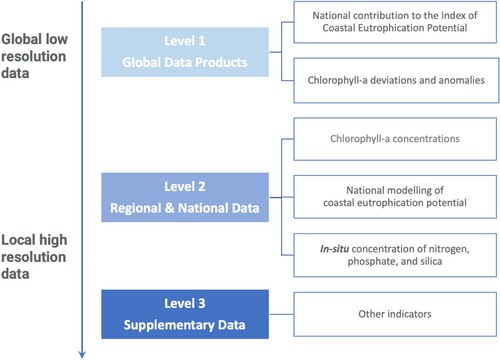
Level 1 sub-indicators utilise globally available data products and consist of a modelled indicator, the ‘Indicator for Coastal Eutrophication Potential (ICEP)’, and two remote sensing-based indicators, ‘Chlorophyll-a deviations and anomalies’ (UNEP Citation2021). The ICEP provides a modelled number indicating the risk of coastal eutrophication at a specific river mouth based on a global level analysis of basin level nutrient exports (total nitrogen, total phosphorus and dissolved silica) to river-mouths (Seitzinger and Mayorga Citation2016; UNEP Citation2021). Then, for Level 2 reporting, national level measurements of chlorophyll-a and other parameters (either in situ or satellite-derived) complement the global remote sensing and modelled data used in Level 1 to enable a more detailed assessment of eutrophication (UNEP Citation2021). Within UNEP SDG reporting context, eutrophication is defined as ‘excess nutrient loading into coastal environments from anthropogenic sources, resulting in excessive growth of aquatic plants, algae and phytoplankton’, hence reformulating the Malone and Newton (Citation2020) and the Nixon (1995) definitions. Furthermore, the Coastal Zone refers to ‘national Exclusive Economic Zone (EEZ) (200 nautical miles from the coast) as outlined by the United Nations Convention on the Law of the Sea’.

This work presents a method to supplement the SDG reporting for 14.1.1a Level 2 sub-indicator chlorophyll-a concentration for European countries in a harmonised, consistent and integrated manner. By using satellite-derived chlorophyll-a data to generate a single variable indicator, we circumvent an issue related to the lack of sufficient data that has plagued previous reporting attempts for European seas (EEA Citation2019b) and global waters (Estoque Citation2020; Alamanos and Linnane Citation2021; Maúre et al. Citation2021). A time series of global daily satellite observations at 1 km resolution extending from 1997 to 2020 (product references 3.1.1 to 3.1.6) minimises temporal and spatial biases in the reporting of coastal eutrophication.

The need for high spatial and temporal monitoring necessitates the use of satellite data to provide a synoptic view. This fundamental requirement underpins our choice of method as well as the one recently adopted by UNEP (Anderson et al. Citation2017; Masó et al. Citation2020; Alamanos and Linnane Citation2021). We compare our proposed methods and results with those obtained by UNEP to identify complementarity, highlight differences, and suggest synergies for further improvement.

3.1.2. Method

The method developed in Pardo et al. (Citation2021) for the North Atlantic Ocean in the 5^th issue of the Copernicus Ocean State Report was extended to derive indicator time series for reporting on potential ocean eutrophication and oligotrophication (PE and PO) in the European regional seas at the EEZ level for consistency with the UNEP progressive monitoring approach ((A)). Annual PE maps were derived for each year and basin using satellite-derived chlorophyll-a concentration from the corresponding CMEMS REP Ocean Colour datasets (product references 3.1.1 to 3.1.5).

Figure 3.1.2. Schematics of the derivation of the SDG14.1.1a sub-indicator on the state of coastal eutrophication. (A) Schematic of the Level 2 approach for the derivation of the annual PE and PO maps and of the chlorophyll-a concentration sub-indicator per Exclusive Economic Zone. (B) UNEP Level 1 approach reproduced with small modification from UNEP (Citation2021).

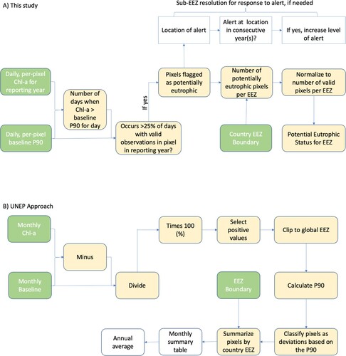
Pardo et al. (Citation2021) developed the PE and PO indicator suite based on the chlorophyll-a 10th and 90th percentiles (P10 and P90 henceforth). The metrics P10 and P90 are considered good indicators to define the baselines of the annual chlorophyll-a cycle, detect the bloom dynamics and to identify high chlorophyll-a episodes (e.g. Gohin et al. Citation2008; Park et al. Citation2010; Groetsch et al. Citation2016; Gohin et al. Citation2020; Pardo et al. Citation2021).

First, to derive the annual PE and PO maps using satellite-derived chlorophyll-a concentration provided in the CMEMS Ocean Colour regional products (product references 3.1.1–3.1.5), daily observations over the year were compared on a pixel-by-pixel basis with the corresponding P10 and P90 climatologies (1998–2017), as in Pardo et al. (Citation2021). For each reporting year, individual pixel values were checked to see if they were above the P90 threshold, below the P10 threshold, or within the [P10, P90] range. If 25% of valid observations within the reporting year for a given pixel were above the P90 threshold, the pixel was flagged as potentially eutrophic condition. Similarly, if 25% of the observations for a given pixel were below the P10 threshold, the pixel was flagged as potentially oligotrophic condition. The method, originally developed for the North Atlantic Ocean (Pardo et al. Citation2021), was extended to all European regional seas: the Mediterranean Sea, the Black Sea and the Baltic Sea, and corresponding PE and PO maps have been derived using the relevant CMEMS Ocean Colour regional products (product references 3.1.2–3.1.5).

Then, new to this work, the PE maps were aggregated for each EEZ per year to derive the 1998–2020 time series for each European country of the Level 2 SDG 14.1.1a chlorophyll-a concentration sub indicator. To this aim, values from the annual PE maps for each EEZ polygon (VLIZ Citation2019) were then extracted from every year ((A)). Annual EEZ mean values were then calculated by performing a spatial average (weighted by pixel area) over the extracted datasets. Finally, annual values for EEZ were presented as a 1998–2020 time series to show the development of the chlorophyll-a concentration sub indicator over time, with each data point representing a European country for a specific year. The EEZs for some countries lie across two basins and hence two different CMEMS regional products. In the case of France and Spain EEZs, the annual data point is a weighted average of the values computed with the North Atlantic and Mediterranean products (product references 3.1.1 and 3.1.3). The same approach was applied for Turkey across the Mediterranean and Black seas (product references 3.1.3 and 3.1.4). Instead, for Sweden the Baltic Product was used (product reference 3.1.5), while for Denmark and Germany only the North Atlantic product was selected (product references 3.1.1).

In the proposed level 2 chlorophyll-a concentration sub-indicator method for European waters, henceforth referred to as the ‘proposed level 2 method’, we have also specifically addressed the treatment of missing data ((A)). In the computation of the baseline climatological P90 and P10 values, we imposed the criterion that at least 5 years out of the 20-year baseline must contain valid data, for these metrics to be calculated. For a particular pixel and day of year, if the number of available observations fell below the threshold, then no further calculations were applied to that location. In computations for the reporting year, if no observations were available for a particular date and location, then it was not possible to calculate differences from the baseline P90 and P10 values for that location and date. In the reporting year, the number of anomalous observations (<P10 or >P90) and the number of valid observations at that pixel for that year were then used to calculate the percentage of occasions when the thresholds were breached. The coverage threshold was set at 50% (half a year) for the reporting year.

Several considerations with respect to the desirable traits of an eutrophication indicator went into designing the proposed Level 2 method presented here. Since eutrophication implies a change from a baseline, it is important to first establish a threshold against which change is measured. This threshold has to satisfy certain criteria. Most importantly, it has to account for natural variability at any given location, including seasonal and interannual variations, because of climate variability. Hence the threshold has to be based on a multi-year baseline, and we have chosen a 20-year baseline, to account for decadal variability. The threshold used here is site-specific, and varies with day of year. Since eutrophication implies an extreme event, we have not averaged over time (weekly or monthly), to avoid smoothing out of extreme events by the averaging process. Eutrophication is a reversible process: if the source of the excess nutrient is cut off, eutrophication can be reversed (EEA Citation2019a). Therefore, for monitoring the effectiveness of measures to improve water-quality, the observed level of eutrophication in one year must be compared against that in subsequent years. This requires a fixed threshold for every location, from one year to the next, and the threshold used here is invariant from one reporting year to the next. Eutrophication implies an increase, over and above the natural variability. Hence our threshold is the 90th percentile for each location, established for a fixed 20-year baseline. In a baseline-like year, we can expect 10% of the observations to exceed P90. Hence, we raise the potential eutrophication indicator flag for a location only if, in any given year, P90 is exceeded in 25% of the available observations. Since the method tests for deviations from the norm over the entire year, it captures both sporadic as well as sustained eutrophication events. We also had to decide whether eutrophication should be established over the growing season or over the entire year. We have opted to monitor for eutrophication over the whole year, to avoid any errors that might be caused from ambiguities in defining a growing season, which can of course vary with location and from year to year.

Within the context of the UN SDG 14.1.1, GEO Blue PlanetFootnote¹ contributed to the drafting of the methodology for calculating the SDG 14.1.1a sub-indicators on chlorophyll-a deviations and anomalies (GEO Blue Planet Citation2021; UNEP Citation2021). The UNEP (Citation2021) proposed method for the Level 1 chlorophyll-deviation sub-indicator based on satellite derived global chlorophyll-a (4 km OC-CCI data, product reference 3.1.6) is illustrated in a schematic manner in (B). The UNEP (Citation2021) method differs from the proposed Level 2 method in the basis and treatment of the P90 estimates and in several other details. Briefly, the UNEP (Citation2021) method uses a fixed 5-year baseline (2000–2004), from which monthly mean chlorophyll-a values are calculated for every satellite pixel. For the reporting year, all local deviations from the corresponding reference mean chlorophyll-a are calculated and noted as relative percent differences. The P90 is calculated for the distribution of positive relative percent deviations of all pixels from the global EEZ of all countries for the reporting month. Pixels with differences that exceed the global P90 for that month of the year are identified as having deviations. Monthly percentage of pixels within each country EEZ with chlorophyll relative percent difference values greater than P90 is then calculated, and averaged over the whole year, as the eutrophication index for that country for the reporting year. For comparison with the proposed Level 2 method, we present the UNEP (Citation2021) results for the European Seas.

3.1.3. Results

presents the annual PE and PO map for 2020 based on CMEMS Ocean Colour regional datasets, visualising where the daily observations over the year were above the P90 or below the P10 thresholds. The indicator map highlights few scattered potentially eutrophic areas in 2020: in the Baltic Sea, the annual PE indicator identified a wide offshore area in the central Bothnian Sea, and also highlighted the coastal waters of the Skagerrak and Kattegat straits, confirming previous trends reported for these problem areas (Andersen et al. Citation2016); in the North Atlantic, areas in the coastal waters of the Norwegian Sea, the Iberian Shelf waters and in the Gulf of Biscay and in Southern Brittany were detected; in the Mediterranean and Black Seas eutrophic status was mainly identified in a narrow coastal strip.

Figure 3.1.3. 2020 annual PE (red) and PO (blue) European method indicator map calculated using the CMEMS Ocean Colour regional products (product references 3.1.1–3.1.5). Active PE flags indicate pixels where more than 25% of the valid observations were above the 1998–2017 P90 climatological reference. Active PO flags indicate locations where more than 25% of the valid observations were below the 1998–2017 P10 climatological reference.

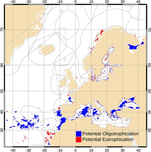
Extensive coastal and shelf waters showed active PO status for 2020: in the North Atlantic large potentially oligotrophication areas were identified in the Iberian Shelf waters, Bay of Biscay, Strait of Gibraltar and the northern coast of Morocco; most of the offshore waters in the Western Mediterranean basin, the Northern Aegean Sea, as well as the western open waters, and the northern and southern coastal waters of Black Sea are classified as potentially oligotrophic. These chlorophyll-a reductions are coherent with the negative trend and anomalies reported in the regional seas (North Atlantic, Mediterranean and Black Sea) for 2020 (CMEMS OMI Citation2020).

The time series of the proposed Level 2 chlorophyll-a concentration sub-indicator method for European waters based on CMEMS Ocean Colour regional products is presented in . The 1998–2020 PE time series shows low percentages across the EEZs with some remarkable PE events occurring in the first decade, with values ranging from 2–4% up to over 20%. In particular, Poland yielded 37.8% in 2008, Bulgaria 25.1% in 2001, Latvia yielded 17.1% in 2008, while Belgium was the only EEZ with two consecutive years above 5%, having reached 15.8% and 23.5% in 2001 and 2002 (). In 2008, four Baltic countries (Lithuania, Latvia, Poland and Sweden) yielded PE values above 7%, thus capturing the extended spring bloom that occurred across the central and southern Baltic Sea and that lasted more than 40 days as reported by Brando et al. (Citation2021).

Figure 3.1.4. Time series (1998–2020) of the PE for European waters based on CMEMS Ocean Colour regional products (product ref. 3.1.1–3.1.5), extending the time series 1998–2019 published in Eurostat (Citation2021). Annual EEZ mean values for each European country were calculated by performing for each year a spatial average (weighted by pixel area) of the annual PE map. AL: Albania, BE: Belgium, BG: Bulgaria, CY: Cyprus, DE: Germany, DK: Denmark, EE: Estonia, EL: Greece, ES: Spain, FI: Finland, FO: Faroe Islands, FR: France, GE: Georgia, GL: Greenland, HR: Croatia, IE: Ireland, IS: Iceland, IT: Italy, LT: Lithuania, LV: Latvia, MC: Monaco, ME: Montenegro, MT: Malta, NL: Netherlands, NO: Norway, PL: Poland, PT: Portugal, RO: Romania, SE: Sweden, SI: Slovenia, UK: United Kingdom.

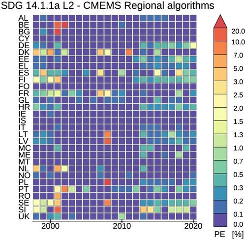
For several countries, the PE at the EEZ level was often nil or never exceeded 1% of the EEZ area (i.e. Albania, Croatia, Cyprus, Faroe Islands, Greece, Greenland, Iceland, Ireland, Italy, Malta, Monaco, Montenegro, Norway, and the United Kingdom, ). Furthermore, from 2013 onwards, most European countries yielded a PE lower than 2%, with the exceptions of Slovenia in 2013–2014 (3.7 and 2.7%) and Spain in 2018 (2.8%). The overall reduction in the PE observed in the second decade of the time series is consistent with the findings by Friedland et al. (Citation2021) based on ensemble analyses for all European seas. These PE results are also coherent with the improvement from 2008 to 2017 in eutrophication status across offshore and outer coastal waters of the Greater North Sea reported for the OSPAR Maritime Area (OSPAR ICG-EUT Citation2017), as well as with the decrease in eutrophication risk recently reported by Gohin et al. (Citation2019) using both in situ and satellite chlorophyll-a data. Furthermore, the PE results for the Baltic countries are consistent with the pattern reported in the integrated annual classification of eutrophication status in the Baltic Sea that described as a time of trend reversal, recovery and oligotrophication in the whole Baltic Sea-wide assessment, particularly in the last decade (Anderson et al. Citation2017; EEA Citation2019a, Citation2019b).

presents the time series (1998–2019) of the UNEP (Citation2021) Level 1 chlorophyll-a deviation sub-indicator computed from the OC-CCI global chlorophyll-a concentrations. The overall ranges differ substantially from as values of the sub-indicators are not directly comparable, but most of the patterns are coherent. Some remarkable chlorophyll-a-deviation events occurring are captured also in . In 2008, five Baltic countries (Poland, Lithuania, Latvia, Sweden and Denmark) yielded values above 8% (with Poland, Lithuania, Latvia exceeding 20%), thus capturing the extended spring bloom that occurred in the Baltic Sea (Brando et al. Citation2021) and already identified in . Furthermore, in 2001 Belgium and Romania yielded 17.1% and 13.9%, respectively, while Portugal reached 17.0% in 2002, and Spain 12.9% in 2015. Minimal chlorophyll-a deviations were identified with the UNEP (Citation2021) method for seven countries yielding less than 2% for most of the time-series (Albania, Cyprus, Croatia, Greece, Italy, Malta and Montenegro, ).

Figure 3.1.5. Time series (2000–2019) of the UNEP (Citation2021) SDG 14.1.1a Level 1 chlorophyll-a deviation sub-indicator based on OC-CCI global chlorophyll-a data (product ref. 3.1.6). Grey boxes identify missing data: reporting was not computed for 1998, 1999 and 2020 (list of countries as for ).

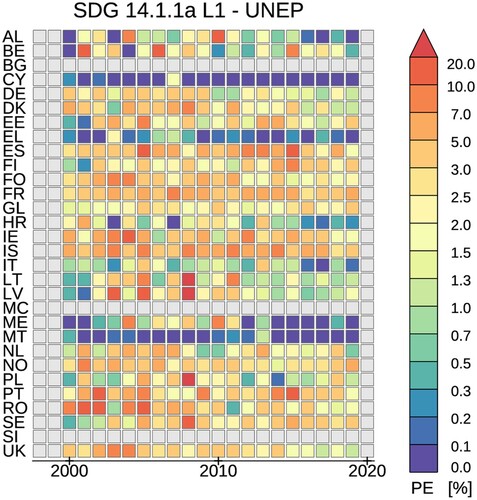
Consistent with and with the literature discussed above (Anderson et al. Citation2017; Gohin et al. Citation2019; EEA Citation2019a, Citation2019b; Friedland et al. Citation2021), also in , it is possible to observe a potential reduction of eutrophication status for the second decade across all European seas. However, it is important to note that the UNEP (Citation2021) method is based on percent differences from the baseline means, and P90 data are calculated from all positive percent differences. This implies that the indicator calculated in this manner may yield some positive values because of natural variability in the system. Therefore, the UNEP (Citation2021) method may identify more potential eutrophication events than the proposed Level 2 method for European waters.

3.1.4. Conclusions

This study presented the refinement and further developments for contributing to the reporting of eutrophication status in the European seas as introduced by Pardo et al. (Citation2021), harnessing the advantages in temporal and spatial coverage offered by remotely sensed ocean colour. We have also carried out some simple comparisons with the UNEP (Citation2021) method’s level 1 sub-indicators.

Several areas were identified as potentially eutrophic or oligotrophic in the 2020 indicator map. However, differentiating transient versus sustained eutrophication and oligotrophication processes may be of interest for management and policy decisions. The time series of the indicator is therefore important to evaluate whether long-term changes are occurring. The PE proposed here provides an estimate of yearly anomalies compared with the regional P90 and P10 climatologies for each EEZ, but it offers no information regarding the spatial location and significance of potential eutrophication and oligotrophication episodes. For understanding of spatial significance, the geographical distribution of the PE and PO, which are provided at the resolution of individual pixels, must be mapped.

The analysis of the time series of the PE over the period from 1998 to 2020 enabled the detection of several eutrophic events occurring mostly in the first decade, followed by an overall reduction in the PE from 2013 onwards. For several European countries, the PE at the EEZ level was often nil or never exceeded 1% of the EEZ area.

For comparison, the chlorophyll-a deviation sub-indicator described in the UNEP (Citation2021) method based on OC-CCI global chlorophyll-a data was calculated for European EEZs. The overall ranges and patterns differ substantially from those retrieved with the proposed level 2 method for European waters as the values of the sub-indicators are not directly comparable, but most of the patterns are coherent.

Reconciling with literature the time series of the PE (retrieved with either method presented here) at an individual EEZ level is problematic, as most papers report phytoplankton phenology, trends and occurrence of eutrophication at the basin or sub-basin level (Colella et al. Citation2016; Anderson et al. Citation2017; Malone and Newton Citation2020; Brush et al. Citation2021; Friedland et al. Citation2021) or for focused coastal marine ecosystems (Zingone et al. Citation2010; Agusti et al. Citation2017; Breitburg et al. Citation2018).

Attempting to monitor eutrophication using only remote sensing chlorophyll-a fields has several limitations. Eutrophication is a process resulting from the supply of excess nutrients, and the remote sensing does not measure nutrients but rather estimates phytoplankton concentration. For this reason, the use of the term potential eutrophication (Maúre et al. Citation2021), was adopted in this study to refer to satellite-derived eutrophication indicators. An increase in chlorophyll-a may indicate an early manifestation of the eutrophication process in the marine ecosystem. The proposed level 2 chlorophyll-a concentration sub-indicator method does not identify the cause of eutrophication, but does provide an alert that increased phytoplankton growth has occurred at the surface, which could indicate eutrophication. We suggest that agencies or organisations utilise the satellite eutrophication indicators to identify areas of potential eutrophication and follow up to investigate the occurrence further, to establish nutrient status and potential causes or sources of nutrient inputs. These methods are capable of providing information about where events occurred within the resolution of the satellite data, nominally 1 × 1 km in this instance. The benefit of satellite data is the ability to gain a synoptic view of potential eutrophication by examining changes in chlorophyll-a in space and time, and the ability to gather data in areas that lack sufficient in situ monitoring. The choice of exploring daily events leaves the method vulnerable to missing data. No analysis or reporting is possible when the number of observations is statistically insufficient either in the baseline years or in the reporting year.

Sustainable stewardship of EEZ may also require information on the level of deviation from P90 and not simply the exceedance of the P90 threshold. Mitigation efforts might also require higher temporal resolution in reporting, such that responsible agencies and organisations are alerted the instant the anomaly occurs. A benefit to using methods based on publicly available remotely sensed chlorophyll-a data from the world’s operational satellite missions is that low latency observations of chlorophyll-a concentrations can be monitored for supplemental information in the interim prior to the calculations of relative indicators.

We conclude that the potential eutrophication and oligotrophication indicators within the proposed level 2 chlorophyll-a concentration sub-indicator method for European waters are an essential component, but not sufficient in isolation, to meet our responsibilities towards sustainable ocean stewardship enshrined in the SDG 14 targets. We acknowledge that indicator methods should continue to evolve with potential improvements to the reporting structure that CMEMS might consider in the coming years. In particular, future work will need to assess the sensitivity of the proposed method to: (i) the monitoring time-window, i.e. over the whole year rather than just the growing season; (ii) the number of valid observations for each year used to calculate the percentage of occasions when the thresholds were breached; (iii) the spatial variability of the exceedance of the thresholds when integrating over EEZs; and (iv) the propagation of the chlorophyll-a concentrations retrieval uncertainties to the potential eutrophication and oligotrophication indicators.

Acknowledgements

The scientific results and conclusions, as well as any views or opinions expressed herein, are those of the author(s) and do not necessarily reflect those of NOAA or the U.S. Department of Commerce.

Section 3.2. Trends in nutrient and chlorophyll a concentrations from FerryBox transect time series in the Baltic Sea

Authors: Samu Elovaara, Sebastian Ehrhart, Seppo Kaitala, Petri Maunula, Jukka Seppälä

Statement of main outcome: The Baltic Sea is heavily eutrophicated because of high, mainly anthropogenic, nutrient inputs from the catchment area. Eutrophication causes ecological and socio-economic impacts so measures to reduce nutrient loads have been implemented. Such policies depend on accurate and abundant monitoring data to implement environmental status indicators reliably. Unattended FerryBox monitoring extends measurements of nutrient concentrations beyond fixed monitoring sites and alleviates the temporal bias of measurements caused by regular monitoring cruises. Our results from a FerryBox transect between Finland and Germany, crossing various sub-basins of the Baltic Sea, capture the seasonal cycle of nutrient concentrations, differences among major regions and individual anomalies on fine spatial and temporal scales. Our data show that inorganic nitrogen (N) and phosphorus (P) concentrations, the nutrients mainly controlling eutrophication, have not decreased during the monitoring period (2007–2020) despite nutrient load reduction efforts. Phosphate and total P concentrations have instead increased slightly in the Gulf of Finland. Dissolved silicate (DSi) concentrations have increased during the past four years in most of the observed sea areas. While DSi concentration does not control eutrophication as much as N and P, it is intimately related to diatom productivity, and through diatoms to sedimentation of organic matter. Thus, better incorporation of DSi into environmental indicators might be warranted. Monitoring the ecological status of the seas would benefit from a multi-platform sampling strategy, as not all scales can be adequately covered by a single platform. FerryBox measurements provide information on fine scale trends in surface waters, as shown here, and should be combined with more traditional monitoring data to better assess the state of our seas.

Products used:

Table

3.2.1. Introduction

Nutrient inputs into the Baltic Sea have been high for decades and most regions of the Baltic Sea are affected by eutrophication (Rönnberg and Bonsdorff Citation2004; Fleming-Lehtinen et al. Citation2008; Andersen et al. Citation2017). Eutrophication remains one of the main environmental problems, despite many measures attempting to reduce nutrient inputs (HELCOM Citation2018a). Conditions unaffected by eutrophication are not expected to be reached unless Baltic Sea Action Plan nutrient reduction targets are met. Even if targets were met some basins would remain eutrophicated for decades to hundreds of years (Murray et al. Citation2019). Therefore, a more detailed understanding of the regional differences, seasonality and long-term changes in the eutrophication process is needed.

Seasonal dynamics between surface water inorganic nutrient concentrations and phytoplankton biomass in the Baltic Sea follows a predictable pattern. Dissolved inorganic N, mainly nitrate (NO₃), inorganic P, mainly phosphate (PO₄), and DSi (SiO₄) accumulate during winter (Snoeijs-Leijonmalm et al. Citation2017). In spring, increased irradiance and stratification initiate propagation of phytoplankton which drains NO₃, PO₄ and DSi pools simultaneously as phytoplankton biomass, most handily measured using chlorophyll a (Chl a), starts to increase. In most parts of the Baltic Sea NO₃ is depleted first resulting in the decline of the spring bloom, leaving excess PO₄ in the water column (Raateoja et al. Citation2011). During the summer, NO₃, and PO₄ remain low, as the thermocline prevents nutrient transfer from deeper layers and abundant phytoplankton communities take up surplus N and P. Later, as irradiance and temperature decrease towards winter, the growing season is terminated and free NO₃, PO₄ and DSi start to accumulate again in the surface waters.

Phytoplankton production in the Baltic Sea is generally N-limited, with some exceptions like the northern low-saline regions (Tamminen and Andersen Citation2007) and freshwater lagoons (Pilkaityte and Razinkovas Citation2007), which are influenced by the high inorganic N:P ratio of riverine water (Savchuk Citation2018). Denitrification of inorganic N (Deutsch et al. Citation2010; Dalsgaard et al. Citation2013) and flux of inorganic P from anoxic sediments and deep waters (Conley et al. Citation2009) maintain low inorganic N:P ratios and N-limitation during the growing season in most regions.

DSi enters the sea mainly through weathering and is taken up by diatoms during the spring bloom. DSi concentrations in the Baltic Sea are assumed to have decreased significantly during the last century due to damming and eutrophication in the catchment area (Humborg et al. Citation2008). While DSi concentration decreases considerably during spring, diatom growth has not yet been considered Si-limited in the main basins of the Baltic Sea (Wasmund et al. Citation2013). However, parts of the Baltic Sea, like the Gulf of Finland and the Gulf of Riga, have been predicted to become silica limited based on previous measurements (Danielsson et al. Citation2008). Traditional diatom-dominated spring blooms have increasingly been substituted by blooms of non-siliceous dinoflagellates in the Gulf of Finland and the northernmost basins of the Baltic Sea (Klais et al. Citation2011) which may affect DSi cycling and have wide-reaching biogeochemical ecological consequences (Spilling et al. Citation2018).

During summer, low inorganic N:P ratios enhance the formation of blooms of filamentous diazotrophic cyanobacteria. These blooms are an annually occurring feature of the Baltic Sea, producing a peak of phytoplankton biomass after the spring bloom and yet another input of N in the surface water, by fixing atmospheric nitrogen (Ohlendieck et al. Citation2000). These blooms benefit from eutrophication and have in recent decades started to appear earlier and increased in intensity (Kahru and Elmgren Citation2014). They now contribute significantly to N-input even in the less eutrophicated Bothnian Sea (Olofsson et al. Citation2021). As some of these species produce toxins, cyanobacterial blooms are considered to be one of the primary nuisances of eutrophication.

To understand and mitigate eutrophication, nutrient dynamics must be examined at relevant spatial and temporal resolution and coverage. Traditional research vessel-based measurements are performed at fixed sampling sites, which enables the generation of long time series at those locations, but often with low temporal resolution. For example, the Finnish national monitoring cruises visit open sea stations four times per year at most (Rantajärvi et al. Citation2020) and timing of these cruises cannot easily be adjusted to match key events in pelagic ecosystems. To analyse shifts in the seasonality or areal patterns, more detailed observations are needed. Spatial coverage of measurements can be expanded cost-efficiently using automated FerryBox sampling systems installed on commercial vessels, so-called ships of opportunities (SOOP). SYKE Alg@line network, which is part of the Finnish national FINMARI RI consortium (https://www.finmari-infrastructure.fi/ferrybox), has been using SOOPs since 1993 (Rantajärvi Citation2003) and currently employs FerryBox systems on two regularly operating ferries; Finnmaid (Finnlines) operates between Helsinki and Travemünde twice a week and Silja Serenade (Tallink) operates between Helsinki and Stockholm daily. The nutrient measurement data collected by these ferries have been included in CMEMS products since June 2021 (product ref. 3.2.1).

In this study, we analysed climatologies of nutrient and Chl a concentrations and their trends in different regions of the Baltic Sea using data collected by FerryBox on the Finnmaid ferry (product ref. 3.2.1) during the period 2007–2020. We visualised the differences in seasonal nutrient and Chl a concentrations on a north–south gradient characterised by increasing salinity and average temperature. The study demonstrates the use of sustained FerryBox data in analysing spatial and temporal trends in nutrient concentrations, at scales unachievable using traditionally collected data.

3.2.2. Methods

Data (product ref. 3.2.1) were collected using the FerryBox installed on the ferry Finnmaid. The system consists of a thermosalinograph, fluorometers for chlorophyll, phycocyanin and chromophoric dissolved organic matter, taking measurements every 20 s, and a temperature-controlled water sampler (Ruokanen et al. Citation2003). The water inlet is at a nominal depth of 5 m. Discrete water samples (24 samples from pre-selected transects) are collected at predetermined locations (as the route is not always the same, water sampling is triggered at fixed longitudinal positions) approximately twice per month and analysed at the SYKE laboratory (Raateoja et al. Citation2018). Nutrient concentrations (Total N, Total P, NO₃, PO₄ and SiO₄) were measured approximately once per month using Lachat QuickChem 8000 flow injection analyser (up until 26.10.2020) and with Skalar SAN++ continuous flow analyser (26.10.2020 onwards) based on Grasshoff et al. (Citation1999). NO₂ concentration is included in NO₃ concentration. Chl a was measured from each sample, extracted using 96% ethanol, and measured fluorometrically, as described in HELCOM (Citation2017). Salinity and temperature were measured continuously within FerryBox using SBE45 MicroTSG thermosalinograph (Seabird) and SBE38 temperature sensor (Seabird), respectively, and the data corresponding to water sampling times was extracted.

Data consist of weekly to monthly sampling sets from 2007 to 2020 on a transect from Travemünde to Helsinki (, Product ref. 3.2.1). Finnmaid took different routes over the years. The route with the most measurement data, passing east of the island of Gotland, was selected. All other routes were discarded from this study. As the sampling positions were not exactly the same for all cruises, they were grouped into zones with a radius of roughly 5 km (hereafter referred to as zones). Zones were created by applying a nearest neighbour cluster search in python (DBSCAN from sklearn, https://github.com/scikit-learn/scikit-learn) resulting in 24 zones. The centres of the zones were assigned coordinates (). The total number of sampling events for each zone varies between 266 and 343, i.e. 19–25 samples per year for each zone.

Figure 3.2.1. Map of the Baltic Sea (excluding northern sea areas) and the shipping route of Finnmaid used for the transect (product ref. 3.2.1). Red points mark the centres of the zones into which sampling locations were pooled. Numbers refer to sub-basins of the Baltic Sea, which are separated by blue lines. 1: Kattegat, 2: Great Belt, 3: The Sound, 4: Kiel Bay, 5: Bay of Mecklenburg, 6: Arkona Basin, 7: Bornholm Basin, 8: Gdansk Basin, 9: Eastern Gotland Basin, 10: Western Gotland Basin, 11: Gulf of Riga, 12: Northern Baltic Proper, 13: Gulf of Finland, 14: Åland Sea.

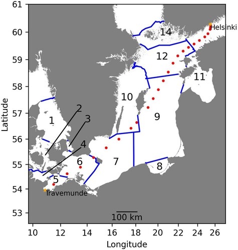
The seasonality within each zone was approximated by binning the values by month of the year and calculating the mean of each bin. This gave an average annual cycle that was subtracted from the 14-year time series of each zone, leaving the long-term trend per zone provided other cyclic effects are absent. The long-term trend within each zone was then fitted with a linear model to estimate the typical annual change of a variable in each zone.

3.2.3. Results

Monthly means of total N, total P, NO₃, PO₄, SiO₄, and Chl a concentrations, temperature and salinity in the surface water capture seasonality and the regional differences covered by the FerryBox transect (). The salinity gradient characterising the Baltic Sea is prominent with higher salinity at the Bay of Mecklenburg and Arkona Basin and lower salinity at the Gulf of Finland ((b)). Chl a concentrations ((h)) and winter accumulation of NO₃ ((e)) and PO₄ ((f)) are higher in the Gulf of Finland compared to the central and southern Baltic Sea, pointing to more severe eutrophication in the Gulf of Finland. NO₃ ((e)) is depleted after the spring Chl a peak (spring bloom), which occurs earlier in the southern part of the transect ((h)) and remains depleted throughout the transect until October-December. Spring consumption of PO₄ ((f)) and DSi ((g)) does not result in full depletion of their pools. Thus, the availability of DSi remains high throughout the year in most regions, especially in the southern Baltic Sea. Depleted NO₃ and availability of PO₄ and DSi suggest that the region covered by the transect is primarily N-limited during the growing season. Summer cyanobacterial blooms are visible in Chl a concentration in June–July especially in the Gulf of Finland ((h)). Based on the depletion and accumulation of NO₃, PO₄ and DSi, and the occurrence of Chl a peaks, the average growing season is approximately 2 months longer in the southernmost end of the transect than in the north.

Figure 3.2.2. Monthly means of temperature (a), salinity (b) and concentrations of total N (c), total P (d), NO₃ (e), PO₄ (f), DSi (g) and Chl a (h) during the entire measurement period (2007–2020) calculated using in situ data collected by Finnmaid FerryBox (product ref. 3.2.1). Observations were grouped into 24 zones (see methods and ) which are presented using the latitude of the centre of the zones.

Figure 3.2.2. Monthly means of temperature (a), salinity (b) and concentrations of total N (c), total P (d), NO3 (e), PO4 (f), DSi (g) and Chl a (h) during the entire measurement period (2007–2020) calculated using in situ data collected by Finnmaid FerryBox (product ref. 3.2.1). Observations were grouped into 24 zones (see methods and Figure 3.2.1) which are presented using the latitude of the centre of the zones.

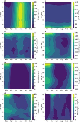
Based on the monthly means, anomalous years were detected showing both extreme events and general trends during 2007–2020 ( and ). The record warm summer of 2018 and beginning of 2020 are visible in the increased water temperature throughout the transect ((a)). Intrusions of high saline water are seen as spikes in the southernmost study area ((b)). Exceptionally high DSi concentrations were measured throughout the transect since 2017 ((g)). DSi concentrations increased at an average yearly rate of 0.3–0.5 µmol L⁻¹ y⁻¹ at each zone except zone 1 compared to the monthly means ((e)). Total P ((b)) and PO₄ ((d)) concentrations also increased during the period 2007–2020, especially in the northern zones. PO₄ concentrations showed high variation and extended periods (several months) of high and low anomalies were detected ((f)). Prominent extended anomalies in the PO₄ concentration can be seen in the southern Baltic Sea (a positive anomaly in 2012 followed by a negative anomaly in 2013–2014, (f)). Total N ((a)), nitrate ((c)) and Chl a concentrations ((f)) have not changed significantly during the period 2007–2020. Greater interannual variations in the concentrations in the northern area likely resulted in a tendency to higher standard errors of trends in that region.

Figure 3.2.3. Deviation of temperature (a), salinity (b) and concentrations of Total N (c), Total P (d), NO₃ (e), PO₄ (f), DSi (g) and Chl a (h) from the monthly means () of the total measurement period (2007–2020) calculated using in situ data collected by Finnmaid FerryBox (product ref. 3.2.1). Observations were grouped into 24 zones (see methods and ) which are presented using the latitude of the centre of the zones.

Figure 3.2.3. Deviation of temperature (a), salinity (b) and concentrations of Total N (c), Total P (d), NO3 (e), PO4 (f), DSi (g) and Chl a (h) from the monthly means (Figure 3.2.2) of the total measurement period (2007–2020) calculated using in situ data collected by Finnmaid FerryBox (product ref. 3.2.1). Observations were grouped into 24 zones (see methods and Figure 3.2.1) which are presented using the latitude of the centre of the zones.

Figure 3.2.4. The upper sub-panel in each panel shows the average annual change from the monthly mean of total N (a), total P (b), NO₃ (c), PO₄ (d), DSi (e) and Chl a (f) during the total measurement period (2007–2020) as a function of the latitude, calculated using in situ data collected by the Finnmaid FerryBox (product ref. 3.2.1). Error bars show the standard error of the fitted long term trend (linear model). The lower sub-panel shows the adjusted R² for the linear fit used to derive the annual change.

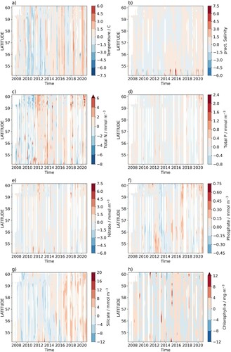
Figure 3.2.4. The upper sub-panel in each panel shows the average annual change from the monthly mean of total N (a), total P (b), NO3 (c), PO4 (d), DSi (e) and Chl a (f) during the total measurement period (2007–2020) as a function of the latitude, calculated using in situ data collected by the Finnmaid FerryBox (product ref. 3.2.1). Error bars show the standard error of the fitted long term trend (linear model). The lower sub-panel shows the adjusted R2 for the linear fit used to derive the annual change.

R² of the linear fits was quite low for all variables (), being highest for DSi (∼0.4 for mid-latitude stations) and total P and PO₄ (close to 0.2 at higher latitudes). R² values were low because there was high variation in the data. As we investigated annual means, i.e. pooled measurements from all the months, the difference in variation among the different seasons (e.g. high values and variation in NO₃ concentration in winter and low in summer) is not included in the model and may contribute to low R² values.

3.2.4. Discussion

Unattended sampling using FerryBox systems on SOOP ferry lines generate vast amounts of data, compared to research vessel-based monitoring cruises. Sampling is cost-efficient and flexible, as the timing, location and frequency of sampling is often adjustable (but constrained by the ferry timetable). On the other hand, SOOP data provides samples from the uppermost surface layer only. So far, SOOP data is not fully exploited in monitoring programmes when assessing the trends of the state of the seas. However, as the use of automated systems for aquatic monitoring is increasing, we need to reconsider how they are included in the monitoring programmes and how to optimise the use of multiplatform data (García-García et al. Citation2019).

FerryBox monitoring can contribute to near real-time diagnosis of changes in pelagic marine ecosystems. Sustained FerryBox data can provide an overview of the spatial extent, timing and duration of events, their interannual variability, as well as long-term trends. This information provides a background for more detailed studies, providing guidance on their timing and positioning to match the events to be studied, e.g. phytoplankton blooms. FerryBox methods do not replace traditional research vessel campaigns which produce much more detailed insight into the ecosystem but supply auxiliary information on the time–space scales.

This study estimated trends in nutrient concentrations using SOOP data in the Baltic Sea. Despite the recent mitigation measures taken these trends are not abating, an observation also supported by HELCOM (Citation2018b). We show that nutrient concentrations in the surface water have changed very little during the past 14 years, with two exceptions. First, there is an increase of total P and PO₄ in the Gulf of Finland, and second, there is an overall increase in the often overlooked DSi concentration.

The observed increase in DSi concentrations contradicts, in the short term, the prediction of decreasing DSi concentration in the Baltic Sea (Danielsson et al. Citation2008; Humborg et al. Citation2008). DSi concentration was very rarely below 2 µmol L⁻¹ which is considered to be growth limiting for diatoms (Egge and Aksnes Citation1992). As PO₄ concentration has also increased in the Gulf of Finland, the inorganic Si:P ratio has not changed much. However, DSi concentration has increased relative to NO₃, suggesting that the already N-limited Gulf of Finland has become relatively less silica limited. Changing Si:N ratios might affect relative nutrient limitation dynamics among diatom species (Spilling et al. Citation2010), thus affecting the composition of the phytoplankton community. We observed increased PO₄ concentrations mainly in the northern part of our study area and towards the end of our measurement period of 2007–2020. However, as shown by Kõuts, Maljutenko, Liu, et al. (Citation2021), PO₄ concentrations for the entire region increased from 1995 to 2000 and have remained high ever since, while nitrate concentrations have decreased. This continuously increased PO₄ concentration relative to NO₃ concentration suggests that cyanobacterial blooms will be an issue for a long time to come, as cyanobacteria gain a competitive advantage in low inorganic N:P ratios (Graneli et al. Citation1990; Stal et al. Citation2003).

It is tempting to link the ongoing decrease in the occurrence of diatom-dominated spring blooms (Klais et al. Citation2011) to the observed accumulation of free DSi. Estimating the magnitude of change in the DSi concentration potentially caused by the community shift is beyond the scope of this study. However, if increased DSi concentration is an indicator of reducing diatom-dominated spring blooms it may also indicate other consequences of reduced diatom dominance on C cycling, such as decreased organic matter sedimentation (Spilling et al. Citation2018), which have been pronounced during recent years.

The increase of both DSi and PO₄ in the Gulf of Finland might also be related to sedimentation processes and introduction of deep water to the surface layer, as variation in benthic DSi and PO₄ fluxes in the Gulf of Finland show similar patterns (Tallberg et al. Citation2017). This suggests a tentative connection between sediment hypoxia and DSi release from the sediments. Hypoxic conditions have been persistent in many regions of the Baltic Sea since 2000 and will possibly become more common in the Gulf of Finland (Kõuts, Maljutenko, Elken, et al. Citation2021). Hypoxia-related DSi and PO₄ release rates thus, cannot be expected to decrease soon. Since P may also be transported from the bottom water of the northern Baltic Proper to the Gulf of Finland, all the way to surface water (Lehtoranta et al. Citation2017), the increased PO₄ concentration in the Gulf of Finland should not be considered to have been caused solely by regional processes.

Throughout the study area, there has been no reduction in eutrophication, as shown by high Chl a concentrations and the lack of a trend in Chl a concentration. The data does not cover the most intense eutrophication period of the Baltic Sea as inputs of N and P have decreased since the 1980s (Gustafsson et al. Citation2012; HELCOM Citation2018a). Therefore, this data can primarily be used to assess how nutrient load reduction measures starting in the 1990s have affected surface water nutrient concentrations. However, nutrient residence times in the Baltic Sea are long, estimated at 9 years for total N and 49 years for total P (Gustafsson et al. Citation2017), and the interconnectivity among basins may compensate for local nutrient reductions (Savchuk Citation2018). This makes it difficult to connect specific nutrient load reduction measures to changes in nutrient concentrations. Long SOOP time series with high temporal resolution may aid in distinguishing these changes from high regional and interannual variation.

Still, the broad-scale spatial differences in nutrient concentrations agree with recent basin and drainage area-specific investigations. Since 1993 a slight decrease in phytoplankton primary production has been detected in the southern Baltic Sea, where Chl a concentrations are generally lower (Zdun et al. Citation2021). Despite nutrient load reduction efforts nutrient input from rivers to the Gulf of Finland remain high as do NO₃ and Chl a concentrations (Räike et al. Citation2020).

Alg@line FerryBox water sample data has been used in HELCOM spring bloom duration and biomass production indices for management purposes. HELCOM used Chl a, dissolved inorganic N and P, total N and P data from FerryBox to create vernal phytoplankton bloom intensity indices connecting them to dissolved inorganic N concentration in the winter (Fleming and Kaitala Citation2006; Raateoja et al. Citation2018). As DSi is generally not considered a limiting nutrient it has not been used as an indicator by HELCOM. However, if increased DSi concentration is partially due to reduced diatom populations, DSi concentration might be considered another potential indicator of the ecological status of the planktonic community. In this case, its possibility to strengthen the diatom/dinoflagellate index might be worth exploring (Wasmund et al. Citation2017). Given the connection between the benthic DSi and PO₄ fluxes (Tallberg et al. Citation2017), DSi concentration could also be used in support of present indicators of sediment hypoxia.

Other potential uses for the data include investigation of nutrient ratios and nutrient limitation, post-spring bloom excess PO₄ and its capacity to fuel summer cyanobacterial blooms (Raateoja et al. Citation2011), and nutrient depletion ratios during phytoplankton blooms. However, studying these may require adjustments in current sampling frequencies and automated nutrient analysis would be an optimal next step for increasing the frequency of FerryBox nutrient sampling.

As FerryBox systems collect high resolution multivariable in situ data in near real-time, they can be an asset to other research approaches. One common use is the provision of assimilation data for biogeochemical models and ocean colour applications. In addition, FerryBox data can be used in conjunction with stationary sampling data to increase data coverage (Raateoja et al. Citation2018). Such an approach could possibly be used to increase the confidence of eutrophication status assessments in the Baltic Sea (Fleming-Lehtinen et al. Citation2015). SOOPs are an integral part of future coastal observation systems to be used in conjunction with stationary sampling stations, other automated systems, remote sensing and modelling, as e.g. in the JERICO research infrastructure (Joint European Research Infrastructure for Coastal Observatories, Farcy et al. Citation2019). Such large-scale joint operations require good communication between the research fields to identify gaps in observation coverage. Within their route limits, SOOPs can modify their sampling programme providing an excellent method of fine-tuning the data collection required by the modelling, remote sensing and management communities.

3.2.5. Conclusions

Annual climatologies and long-term trends of nutrient and Chl a concentrations from 2007 to 2020 covering a north–south gradient from Helsinki to Travemünde were presented. Chl a concentration has remained the same throughout the transect, suggesting that eutrophication has not been alleviated in this area. Concentrations of PO₄ and especially DSi have increased over the past 4 years when compared to 2007–2020 monthly averages. Increased PO₄ concentrations demonstrate how slowly the surface water PO₄ concentrations react to nutrient load reduction efforts as new PO₄ is released from the sediments. Systematic increase of DSi concentrations in major basins of the Baltic Sea might be a reason to consider DSi concentration as a potentially important environmental indicator. This is especially important, because the changing DSi concentration may be related to a major ecological change in the Baltic Sea, the shift from diatom to dinoflagellate-dominated spring blooms. We consider the high spatial resolution and temporal coverage of FerryBox data to be an important component in the sustained analysis of nutrient concentrations and eutrophication.

Acknowledgements

The study utilised SYKE Alg@line FerryBox infrastructure as a part of the national FINMARI RI consortium. We thank two anonymous reviewers for their constructive comments and Danielle Bansfield for language editing.

Funding

The work has been supported by JERICO-S3 project, funded by the European Commission's H2020 Framework Programme under grant agreement No. 871153 and by the Academy of Finland (SEASINK: Evolving carbon sinks and sources in coastal seas - will ecosystem response temper or aggravate climate change?).

Section 3.3. Copernicus Marine Sea Surface Temperature and chlorophyll-a indicators for two Pacific Islands: a co-construction monitoring framework for an integrated, transdisciplinary, multi-scale approach

Authors: Alexandre Ganachaud, Karina von Schuckmann, Andra Whiteside, Cécile Dupouy, Pierre-Yves Le Meur, Maeva Monier, Simon Van Wynsberge, Antoine de Ramon N’Yeurt, Maria Mañez Costa, Jérôme Aucan, Annette Breckwoldt, Louis Celliers, Pascal Douillet, Sebastian Ferse, Elisabeth Holland, Heath Kelsey, Vandhna Kumar, Simon Nicol, Maraja Riechers, Awnesh Singh, David Varillon

Statement of main outcome: The ocean is an integral part for the three pillars of sustainable development: environment, society and economy. Pressures on the ocean from climate change, pollution, and over exploitation have increased over the past decades, posing unprecedented challenges, particularly for vulnerable communities such as the Large Ocean Island States, and these pressures need to be monitored. This study analyses the time series of Essential Ocean Variables sea surface temperature and chlorophyll-a in coastal reefs of two pilot regions in Fiji and New Caledonia. In situ measurements represent true local conditions, with a necessarily limited coverage in time and space. Remote sensing data have a broad coverage but are necessarily limited in terms of resolution and accuracy in the coastal zone. Our analysis points to the advantage in using these complementary data types for the same geographical areas at small spatial scales close to the coast, and in particular, for high frequencies and extreme events. We discuss the way forward for a co-constructed monitoring framework, drawing on ongoing initiatives in Oceania, and advocate a methodology for the use of ocean data to support society and economy. Co-construction with stakeholder involvement is paramount for this framework, including policy- and decision-makers, industry, scientists, local and indigenous, governmental and non-governmental organisations, all of whom need sound, multi-disciplinary science advice, targeted expertise, and reliable evidence-based information to make informed timely decisions for the right timescale. Such transdisciplinarity combines scientific, traditional, administrative, technical, and legal knowledge repertories.

Products used:

Table

3.3.1. Introduction

Pressures on the ocean from climate change, pollution, and over-exploitation have increased with a growing world population and over time. With continued environmental stress on the ocean in response to ongoing global warming (e.g. IPCC 2019b, Citation2021), as well as with the prospective development of new ocean-related economic activities, these problems are only expected to further exacerbate (OECD Citation2020). The ocean is integral to Small Island Developing States’ (SIDS) economies (Dornan et al. Citation2018; Keen et al. Citation2018) as their vast Exclusive Economic Zones are much larger than their actual land space (70-fold in Fiji, Gassner et al. Citation2019), and Pacific islanders have proposed to shift the terminology from SIDSs to Large Ocean Island States (LOIS) (Hau’ofa Citation2000; Morgan Citation2021). The SIDS/LOIS are particularly exposed to anthropogenic pressure on the ocean due to low elevation, small land area, narrow ecological zonation, climate sensitive ecosystems and natural resources; insufficient financial, scientific and technical capacities; unique social and political conditions, proportionally (compared to mainland countries) more limited human resources, and local and unique forms of bureaucracies (Magnan et al. Citation2019).

Globally, ocean knowledge is of great benefit to inform policy, decision making, governance and management and therefore to increase the likelihood of developing sustainability (Colglazier Citation2018; Hermes et al. Citation2019; Kaiser et al. Citation2019). The concept of Essential Ocean Variables (EOVs) as implemented by the Global Ocean Observing System (GOOS) is based on relevance for climate and ocean services, including ocean health (Le Cozannet et al. Citation2017; Le Traon et al. Citation2017), and considering feasibility, maturity of the science and measurement techniques, and cost effectiveness (Lindstrom et al. Citation2012). Similarly, the framework of Global Climate Indicators as introduced by the World Meteorological Organisation (WMO Citation2017) in the light of SDG 13 ‘Climate action’ includes a subset of key indicators – many of them ocean-related – designed to be comprehensive and understood by non-scientific audiences, and form the basis of their annual Statement of the State of the Global Climate (e.g. WMO Citation2020) used amongst others by the UN Framework Convention for Climate Change. Within the large scale or global processes, the need to include local and indigenous knowledge in adaptation planning and adaptive management remains a challenge (Celliers et al. Citation2021).

Sea Surface Temperatures (SST) and Chlorophyll-a (Chl-a) are EOVs for the Earth’s ocean system (O’Carroll et al. Citation2019; Sathyendranath et al. Citation2019). SST impacts marine ecosystems. Satellite derived SST anomalies, and derived indicators (e.g. degree heating weeks (DHW) coral bleaching alert) directly provide relevant information in near-real time that can be used by managers. Monitoring and forecasting local thermal regimes are important for understanding and protecting potential refugia for coral species (Foo and Asner Citation2020; Schoepf et al. Citation2020), or managing aquaculture activities (Van Wynsberge et al. Citation2020). For instance, a warning of abnormal conditions is useful to initiate more intensive in situ monitoring, or prepare for action in case of bleaching (Heron et al. Citation2016; Andréfouët et al. Citation2018; Sully et al. Citation2019; Skirving et al. Citation2020).

The EOV Chl-a is a proxy for the amount of photosynthetic plankton in the ocean, which is an indicator of carbon uptake, productivity and overall health of the ocean (e.g. Martinez et al. Citation2009; Mélin et al. Citation2017). Together with nutrients and suspended sediments, Chl-a is also an indicator of water quality, one of the pressures on vulnerable ecosystems such as the seagrass beds and coral reefs (Devlin et al. Citation2020; Vollbrecht et al. Citation2021). At the local scale, it is used to monitor changes in coastal lagoon water quality (Dupouy et al. Citation2018a; Vollbrecht et al. Citation2021); it also impacts larval recruitment (Wilson et al. 2018). For instance, Putra et al. (Citation2021) showed that most of the potential fishing ground in Riau Islands (Indonesia) were linked to Chl-a increases associated with different monsoon types. Understanding the drivers of Chl-a variations is therefore important to marine spatial planning efforts and managing marine ecosystems, but the access and ability to make use of such data around Fiji are not yet available to stakeholders (Gassner et al. Citation2019; MACBIO project – Marine and Coastal Biodiversity in the Pacific Island CountriesFootnote²).

Here we analyse SST and Chl-a, as measured at regional (remote sensing/CMEMS products) and local (in situ) scales in two Pacific Islands, Fiji and New Caledonia, to provide insights about CMEMS products’ usefulness and limitations for local ecosystem management. These products are often developed for broader applications and not designed for specific local needs. In our discussion, we, therefore, advocate the importance of a local, specific and transdisciplinary approach to co-construct data products that best serve scientists, administrations, authorities, managers, business, and local communities to support ocean sustainability in the long term. We discuss future ways to tackle the missing elements (plural knowledge and norm repertoires of various actors) in the construction of relevant indicators and monitoring frameworks.

3.3.2. Two EOV indicators in Fiji and New Caledonia

3.3.2.1. Data used

For SST, we used large-scale satellite observations from the ESA CCI project (product ref. 3.3.5). This satellite-derived SST product provides a bulk SST, equivalent to water temperature at 20 cm below the sea surface (Product ref. 3.3.5). We will refer to it as SSTSAT. The inputs to the system are SSTs at 10:30 am and pm local time which means that the SST provided by this product roughly corresponds to the daily average. SSTSAT anomalies are relative to the daily SSTSAT climatology from January 1st to December 31st of the ESA CCI data period. SSTSAT extracted from the product were used directly, without any further processing. The SSTSAT values from this product were compared to local in-situ SST observations for Fiji and New Caledonia using sites from the ReefTEMPS observing network (product ref. 3.3.6), which is part of the French Research Infrastructure for Coastal Oceans and Seashores (ILICO), and also known as the Pacific Insular Coastal Waters Observation Network. ReefTEMPS consists of a number of monitoring platforms at 6–60 m depth scattered around 20 Pacific Island countries, with 30 monitoring stations in New Caledonia, and 11 in Fiji (Cheype et al. Citation2015; Cocquempot et al. Citation2019; Varillon et al. Citation2021). For the purpose of the current analysis, one station in Fiji and four in New Caledonia were selected to maximise the mutual temporal coverage of remote sensing and in-situ measurements.

For Chl-a, we jointly use four different data products, i.e. a monthly gridded (product ref 3.3.1) and daily non-gridded CMEMS (product ref 3.3.2) remote sensing, the CMEMS Ocean Monitoring indicator (product ref 3.3.4). These Chl-a satellite products are designed for open ocean use – what are called Case 1 waters whose optical signal is dominated mainly by phytoplankton present at low concentrations – and are not designed to be used in optically complex coastal waters – called Case 2 waters (IOCCG Citation2000). Lagoon waters would require adapted algorithms such as the one issued from the comparison of MODIS and in situ Chl-a concentration coincidences all around New Caledonia (Case 1 and 2 waters, Wattelez et al. Citation2016) and that are yet to be applied to other lagoons. Therefore, only CMEMS data offshore (Case 1 waters) were selected for this study, and only the evolution of offshore waters is discussed. These are compared with in situ data collected during five oceanographic cruises South of Fiji from 2001 to 2004 (Bula programme, by IRD / UR CAMELIA, ANSTO and U. South Pacific, product ref. 3.3.3). In-situ Chl-a data were measured after filtration on a 0.7 µm GF/F filter and extraction of the phytoplankton retained in methanol (Chifflet et al. Citation2004). In addition, a Chl a data point south of the region (178.79° E, 18.48° S) was used to represent the ‘bluest water’ (product ref. 3.3.7).

3.3.2.2. Regional results from satellite products

3.3.2.2.1. Ocean temperatures

Over the periods that span available in situ data, SSTSAT changes are characterised by surface warming around Fiji and New Caledonia between 2013 and 2019 ((a)), and in the north-eastern part including Fiji between 1997 and 2019 with more than 0.02°C per year ((b)). For comparison, global mean SST increased at a rate of 0.015 ± 0.001°C per year over the period 1982–2019 (CMEMS Citation2021b). In contrast, the area north-east of New Caledonia ((b)) showed cooling conditions over the period 1997–2019 at rates of around −0.01°C per year, while the area south-west of New Caledonia showed surface warming conditions over this period, at rates between 0 and 0.02°C per year. Cravatte et al. (Citation2009) and Quinn et al. (Citation1998) found such strong spatial variability in ocean surface warming over many time scales (see also Sun et al. Citation2017). In the western tropical Pacific, SST vary strongly with the modes of the El Niño Southern Oscillation at interannual time scales, thereby influencing trend calculations over these short periods (e.g. Gouriou and Delcroix Citation2002).

Figure 3.3.1. SST & Chl-a: Trend of Sea Surface Temperature (average yearly anomalies) as derived from product ref. 3.3.5 over the period (a) 2013–2019 and (b) 1997–2019 (units: °C per year). The two periods have been chosen to overlap with the availability of in-situ records. Coloured circles indicate corresponding trend estimates as derived from in-situ observations (product ref. 3.3.6, see ). Note the difference in colour scales in the two plots (c) Chl-a trend (units: % per year) over the period 1997–2019 from product ref. 3.3.3. White pixels are not statistically significant.

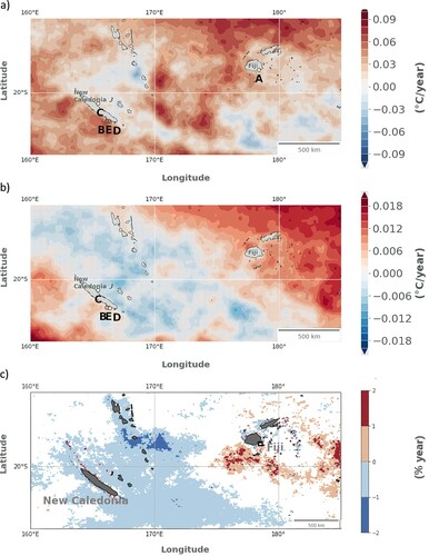
3.3.2.2.2. Chl-a

The Chl-a trend over the period 1997–2019 is characterised by a decrease between the New Caledonia and Vanuatu archipelagos of more than 1%, and an increase south of Fiji at rates of more than 1% per year ((c)). These trends in biomass of phytoplankton are weak relative to global ocean changes (− 6–10% per year, CMEMS Citation2021a) and regional Western Pacific changes (−3% to 3% for the same period, Holland et al. Citation2019). Observations of either a decrease or an increase of Chl-a towards an island in different archipelagoes of the Western tropical Pacific have been attributed to island mass effects (Dandonneau and Charpy Citation1985). Such variations in Chl-a may originate from a large range of triggering factors including physical environment changes altering the supply of essential nutrients, already found at a large scale in the Pacific Ocean (Dupouy et al. Citation2004; Martinez et al. Citation2009). Chl-a trends might also result from changes in phytoplankton species which have different optical properties (e.g. an increase in the proportion of diazotrophs vs picoplankton, a major component of phytoplankton in the region; Dupouy et al. Citation2018b). Evaluating phytoplankton composition change over this long period of time would require algorithms for discriminating phytoplankton groups based on CMEMS reflectance observations (IOCCG Citation2021).

3.3.2.3. Regional to local results: Comparison with in situ data

3.3.2.3.1. Ocean temperatures

SSTSAT trends compared well with in-situ observations during both overlapping study periods ( and ). However, pointwise examination of the time series reveals a small, systematic underestimation in satellite data. For example, the Suva Reef (Viti Levu Island, Fiji) recorded an in-situ warming rate of 0.024 ± 0.01°C per year (December 2012 to December 2019), whereas the satellite-derived estimate is barely significant at 0.009 ± 0.007 (). For New Caledonia at Poindimié, which is located in the north-eastern part of the country, the surface ocean warming trend is non-significant over the 25 years from both in situ and SSTSAT (). These in situ variations in local trends are related to the large spatial variability in trends () and to numerous local effects, combined with a high variability at interannual timescales (Quinn et al. Citation1998). At the southwestern part of New Caledonia, both stations Uitoe01 ((b)) and Anse Vata ((b)) show surface warming rates close to the global mean average, with Anse Vata covering the period February 1958 to early 2020. Rates of temperature change as derived from the satellite data underestimate the warming at these locations, in particular at Anse Vata (−36%) and Viti Levu (−62%).

Table 3.3.1. In situ temperature meta data and correlation coefficients for the comparison with SSTSAT. Station positions on regional scales, and overlapping time series lengths are provided in and , respectively. The significance level at 95% would be 0.55 if we had only 10 independent samples and 0.38 for 20 samples. Maps are based on Etopo5 in Fiji, and a high resolution SHOM DEM in New Caledonia.

Display Table

Table 3.3.2. Trend calculations during overlapping periods for SST time series from in situ reef loggers (ref 3.3.6) and the remote sensing product (ref 3.3.2).

Daily satellite and in situ time series correlations are all above 0.75, well above the significance level (). The maximum correlation was found for the logger deployed on the reef slope at Poindimié (0.87), which is of the same order of magnitude as correlations found between SSTSAT and coastal temperature reported by other coral reef studies (Smale and Wernberg Citation2009; Van Wynsberge et al. Citation2017; Gomez et al. Citation2020). With respect to extreme amplitudes, the coloured, regular peaks in with the overlain satellite series in grey shows a prominent underestimation by satellite products. For a ‘hot extreme’ definition at two standard deviation, SSTSAT is on average lower by 0.9°C (Uitoé); 0.7° (Vata); 0.4° (Prony); 0.4° (Viti Levu) and 0.3°C (Poindimié), with common excursions at 2°. Equivalently, SSTSAT can overestimate cold temperature by up to 4°C. Previous studies concluded that differences between SSTSAT and temperature recorded by in situ sensors deployed on outer reef slopes or in open and exposed lagoons were mostly due to vertical stratification (including a skin effect) of water and localised upwelling along the reef slope that generates lower in situ temperature than SSTSAT (Sheppard Citation2009; Castillo and Lima Citation2010; Claar et al. Citation2020). These processes are unlikely to generate an underestimation of satellite-derived products which, particularly during summer months, are likely to result from higher variability in shallow coastal waters (see, e.g. the shallower sensor D-NCL Anse Vata located near the coast). This higher variability of temperature at local scale could not be captured by the spatial resolution of SSTSAT products (Stobart et al. Citation2008; Van Wynsberge et al. Citation2017; Gomez et al. Citation2020; Van Wynsberge et al. Citation2020). The underestimation of extremes that we find here requires further analysis and needs to be adapted to relevant extreme indicators, e.g. DHW versus anomalies (see subsection 3.1 below) ().

Figure 3.3.2. Time series of daily in-situ SST anomalies at some measurement platforms (coloured lines) in Fiji and New Caledonia of the ReefTEMPS observing network (product ref. 3.3.6). Station locations (a) Suva Reef, Viti Levu, Fiji; (b) Uitoe01, New Caledonia; (c) Poindimié, New Caledonia; (d) Anse Vata, New Caledonia; (e) Prony, New Caledonia] are indicated in the maps of . Satellite derived daily SSTSAT (product ref. 3.3.5) anomalies closest to each measurement platform have been added, respectively (grey line). Anomalies were calculated with respect to the annual climatology over the overlap periods.

3.3.2.3.2. Chl-a

Just south of Fiji ((A)), daily ((B)) and monthly ((B)) images depict differences during the months of April and September within the same year. These two dates were chosen to illustrate a case of high Chl-a (> 0.6 mg.m-3) south of Fiji, extending as a large plume off the coast towards the South (April), and a case of low Chl-a (< 0.4 mg.m-3) and no plume (September). For comparison, tropical oligotrophic open ocean Chl-a ranges from 0 to 0.35 mg.m-3 (Dupouy et al. Citation2018b). For the dates of the Bula cruises, CMEMS daily data were available only on September 2, 2003. Very few daily non-gridded data (product ref 3.3.2, (B)) are available due to heavy cloud cover over this highly convective region, in particular over land and near coasts (Vincent et al. Citation2011). As a result, we had to rely on the monthly gridded composites (product ref 3.3.4) for our comparison with in-situ Chl-a observations.

Figure 3.3.3. Chl-a observations: (A) Study area (black outlined box) in proximity to the wider Fiji zone, with Chl-a change (from product ref 3.3.1) (B) Chl-a in the proximity of Fiji in April and September 2003 for the day of the Bula cruise (product ref 3.3.2). In situ data are represented by the coloured circles, on the same colour scale (product ref 3.3.3) (C) Same as (A) based on the monthly Chl-a product (product ref 3.3.1), for April 2003 and September 2003. The two off-shore stations discussed are station 29 and station 48. Station 54 was discarded because of the Rewa river influence. The black dot to the south (178.79°E, 18.48°S) in ‘bluest water’ corresponds to a station sampled on October 2009 (product 3.3.7).

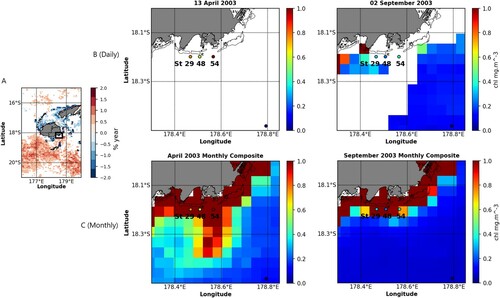
Among the Bula cruise data, two stations (St 29 and St 48) were sampled in open waters (Case 1 waters, behind the reef passages in (B,C)). April and September monthly CMEMS products show Case 2 waters (in brown) near the coast. To avoid contamination by land in the CMEMS Case 2 waters, we selected pixels directly to the south of those stations for our comparisons. Station 54 is at the same distance from the coast, but was discarded because it is under the influence of the Rewa river output (Singh and Aung Citation2008) with high variability in Chl-a values linked to heavy and episodic sediment loads (Fichez et al. Citation2006).

Monthly satellite and instantaneous in-situ Chl-a for stations 29 and 48 are correlated despite the high temporal and spatial interpolations or smoothing ((a)). The correlation is significant at 99% (r²= 0.47, N = 11) ((b)).

Figure 3.3.4. (a) Chl-a time series of monthly satellite-derived CMEMS Chl-a (product ref. 3.3.1) south of the position of the Bula stations 29 and 48 (grey bullets ‘Southern Pixels’), and in situ Chl-a (product ref. 3.3.3) measured by fluorimetry (open squares) for the 5 Bula cruises (Bula 1: 6–11 Nov 2001, Bula 2: 12–19 March 2002, Bula 3: 12–22 May 2003 Bula 4: August 30–September 9, 2003; Bula 5: 5–15 June 2004) and for the S288 Seamans October 2019 cruise (b) Linear regression graph for Bula + Seamans data.

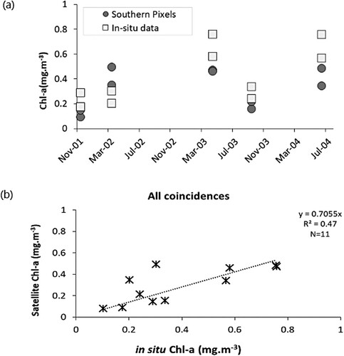
Temporal evolution of monthly satellite Chl-a at these stations during the 1997–2021 period shows. An increase in variability of Chl-a in 2007 and 2011 at all stations (). The generally higher mean Chl-a value at station 54 (mean Chl-a = 0.53 mg.m⁻³) confirms the impact of the Rewa river episodic runoffs. It superimposes with seasonal and interannual cycles observed at stations 29 (mean Chl-a = 0.37 mg.m⁻³) and 48 (mean Chl-a = 0.47 mg.m⁻³). The Rewa River also increases the number exceedances of a 0.53 mg.m⁻³ threshold: 33% of the time for station 54, 24% for station 48 and 5% for station 29. In contrast, the reference point far south of the 3 stations experiences low Chl-a and a more regular seasonal cycle.

Figure 3.3.5. Satellite-derived monthly Chl-a (ref. 3.3.1) at a pixel just south of the in-situ stations st 29, st 48, st 54 and our reference point to the south (see (B)). St 54 is heavily impacted by the Rewa river and therefore not included in the correlation analysis. Variability is much lower at the reference point to the south. The red and blue dots indicate in the Bula situ data (ref. 3.3.3).

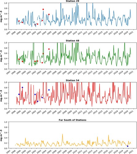
3.3.3. Discussion

3.3.3.1. Strengths and weaknesses of the EOV SST and chl-a products as indicators

We used five pilot sites in New Caledonia and Viti Levu in Fiji to provide insights about CMEMS SSTSAT and Chl-a products strengths and limitations (subsection 3.3.2.2.3 above) for potential application in an ecosystem monitoring and management framework. We found that the bias in SSTSAT products is important when considering extreme events, but acceptable when characterising long-term local changes, with respect to previous studies that find stronger biases (e.g. Sheppard Citation2009; Castillo and Lima Citation2010). This may be explained by the fact that these sites are either well-flushed with open-ocean waters (sites B-NCL, C-NCL, and A-Fiji), or face a lagoon that includes SSTSAT product pixels (sites D-NCL & E-NCL). Trend biases found here may therefore be unrepresentative of other reef and lagoon configurations that can be encountered in the Pacific region. Extreme warm ocean temperature, or ‘Marine Heat Waves’ (Holbrook et al. Citation2019; Oliver et al. Citation2021; Dayan et al. Citation2022; de Boisseson et al. Citation2022), which have major influences on ecosystems, are underestimated although their observation and predictions are essential for marine managers for adaptation and mitigation efforts. Specific analyses are necessary to assess precisely the relation between in situ and satellite-derived time series extremes (Holbrook et al. Citation2019).

SSTSAT products can provide gridded data on a quasi-real time basis, offering both adequate spatial and temporal resolution. The highest spatial resolution gridded product (L4) is 1 km (Merchant et al. Citation2019, product ref. 3.3.5), but its effective resolution is coarser. It is relevant for sufficiently wide water bodies (Van Wynsberge et al. Citation2020) but not for many coastal areas, in particular the complex lagoons and coral reefs relevant to the monitoring aspirations of this study. In contrast, in situ temperature loggers provide high accuracy on a small-scale local level. For coral bleaching applications, in-situ loggers can detect very localised temperature peaks caused by poor water circulation, local weather conditions, and water column stratification, or mass exchanges between inner lagoons and outer reef areas. Loggers, however, often provide short time series or series affected by gaps which limit their use for monitoring climate change. To properly describe a given coastal area for monitoring purposes, sensors must be deployed to capture a diversity of depth and reef locations, though very few have real-time transmission possibilities, which limits their practical use in many remote coral reefs. Modelling in situ temperature from SSTSAT on the basis of (shorter) temperature time series from loggers (Van Wynsberge et al. Citation2017) provides a promising downscaling approach to reconstruct long time series at the very local scale, but must be performed case-by-case to account for local specificities in hydrodynamics, reef configuration as well as lagoon size and depth (Van Wynsberge et al. Citation2017; Reid et al. Citation2020).

Our results have also explored the relevance of Chl-a products to environmental management. Ocean colour offshore the barrier reefs and south of the Fiji in-situ stations provides the decadal trends and responses of phytoplankton biomass through its Chl-a concentration. The observed increases in Chl-a may originate from the influence of terrestrial inputs such as sediment and dissolved organic matter transports, and ultimately can trace the dissemination of contaminants and responses of pelagic communities to increased nutrient inputs around Fiji (Fichez et al. Citation2006; Gassner et al. Citation2019), with potential effects on fish species and fish recruitments in offshore waters around the Fijian reefs. Chl-a increases can also indicate a change in phytoplankton composition (Dupouy et al. Citation2018a). As for temperatures, the biological activity and associated coastal water colour are influenced by many factors including small scale oceanic processes, human activities and sediment input, and it remains critical to relate satellite data to in situ data before any usage in a monitoring framework.

In situ Chl-a data are much harder to acquire than temperature data, and therefore rare. Our Fijian case study illustrates that a monthly CMEMS Case 1 product partially reproduces the in-situ, instantaneous data for the 5 dates considered here. Case 2 Chl-a pixels were not used as they require different and adapted algorithms. Despite its design for large scale applications, the monthly CMEMS product shows a significant relationship with the limited coastal in situ data set that is available ((b)), with some biases. It may therefore contain temporal and spatial information on oceanic variability around the islands, but its further use for monitoring is subject to validation with in situ Chl-a.

Our analyses of temperature and Chl-a time series therefore point to the advantage in having both in situ and remote sensing data for the same geographical areas. In-situ data are essential for accuracy monitoring at small spatial scales (e.g. local reef temperature, coastal ocean water quality), and in particular for extreme events. In situ measurements represent true local conditions, but with a necessarily limited coverage in time and space; whereas remote sensing data have broader coverage but are necessarily limited in terms of resolution and local accuracy. The corresponding data products and interfaces need therefore to be design according to local needs, as we discuss below.

3.3.3.2. A potential way forward: A co-construction monitoring framework using an integrated, transdisciplinary, multi-scale approach

Unprecedented and amplified impacts of ocean climate change occur at local scales, and adaptation measures (including socio-technical, political, cultural and or institutional innovations) and strategies need to be informed and designed at the regional and local levels. Actions need to be implemented in an integrated, transdisciplinary and multi-scale framework (Máñez Costa et al. Citation2017; Rölfer et al. Citation2020; Celliers et al. Citation2021). The UN Decade of Ocean Science for Sustainable Development provides a foundation to help achieve this objective and to ensure science responds to the needs of society ‘to reverse the decline in Ocean health’ by promoting codesign approaches (Ryabinin et al. Citation2019; GOOS Citation2022). Ocean products that are designed under global frameworks offer critical insights on general ocean change, variability and their drivers, but it may either be under-utilised or mis-utilised at local scales for various reasons: (1) other factors may need to be considered when working on mitigation or adaptation of an ecosystem (ecosystem/nexus approach); (2) the understanding by local actors about ocean climate change consequences may differ substantially from the scientific understanding underpinning the global monitoring frameworks; (3) local specificities challenge the downscaling or upscaling techniques; and (4) potential consequences can generate unanticipated and negative local effects.

To address these issues in Oceania and following Belmont Forum and Ocean Decade initiatives, we promote here the following considerations for stakeholders, including scientists, public officers and citizens of the Pacific Islands to share common objectives and actions in order to achieve environmental sustainability when designing monitoring systems:Footnote³

Ecosystem approach (Skern-Mauritzen et al. Citation2016; Liu et al. Citation2018): Consideration of an ensemble of stressors, including environmental, socio-economic, cultural and political aspects (Zhang et al. Citation2021).
Shared understanding: Local understanding and representation climate change impacts depends on knowledge, values, drivers, barriers and opportunities. The accessibility and utility of products for stakeholders needs to come with a shared understanding of climate change impacts and indicators (Kaiser et al. Citation2019; Mackenzie et al. Citation2019; Vargas-Nguyen et al. Citation2020).
Scalability in coastal areas: Globally based indicators may miss important issues as revealed by local experience and combining and matching needs and knowledges produced at different scales and from different ontological viewpoints entails combining heterogeneous elements that cannot be ‘added’ to one another in many cases (‘non-scalability’) (Tsing Citation2012, Citation2015), nor generalised to other places (see Bergthaller et al. Citation2014 on ‘the practice of environing’).Footnote⁴
Forecast ethics: Delivery of forecast products can have heavy consequences, given uncertainties, or generation of inequalities from unbalanced capacities to use it, and therefore needs to come with ethical considerations that include engagement and equity for end users (Hobday et al. Citation2019).

To produce those relevant indicators, extend existing EOVs (or implement new EOVs), and build interest and ability to use them, bottom-up driven consultations and developments are essential steps (e.g. Claudet et al. Citation2020). Such participative framework can foster an enriching dialogue, provide new insights about socio-ecological processes, and contribute to augment the perception of unprecedented ocean changes (Johannes Citation1981; Hviding Citation2005; Singh et al. Citation2021). Indigenous peoples and local communities (IPLC) can actively contribute to the process.Footnote⁵ For instance, IPLC knowledge in combination with remote sensing allowed efficient mapping of the tropical marine habitat of the Solomon Islands (Lauer and Aswani Citation2008). Combined analysis of fishermen’s local knowledge with remote sensing data for SSTSAT and Chl-a can lead to participatory mapping of fishing grounds (Rahimi bin Rosli Citation2017; Mason et al. Citation2019) and support marine conservation and management (Aswani and Hamilton Citation2004; Aswani and Lauer Citation2006). (See McNamara et al. (Citation2020) and Chambers et al. (Citation2021) for a review of such co-constructed projects for sustainability.) The identification and synthesis of data and knowledge sources by structured consultation with project partners, scientists, and stakeholders is therefore needed to take the next steps toward a co-designed monitoring framework (Vargas-Nguyen et al. Citation2020), including locally based and globally produced knowledge (Hviding Citation2003; Strang Citation2009; Sterling et al. Citation2017).

In Oceania, these efforts will come in support of ongoing projects, in particular, the SPC-lead Pacific Community Centre for Ocean Science (PCCOS) programmeFootnote⁶ for delivering integrated scientific services supporting ocean management, governance and observations; the Pacific Data HubFootnote⁷ as well as the Digital Earth PacificFootnote⁸ that aim at gathering available data and make it available for Pacific Member States to make more informed decisions and report their progress toward the United Nations SDGs,Footnote⁹ and the recent USP/UNC Master in sustainability.

Section 3.4. Consistent data set of coastal sea level: The synergy between tidal gauge data and numerical modelling

Authors: Sebastian Grayek, Emil Stanev, Nam Pham, Antonio Bonaduce, Joanna Staneva

Statement of main outcome: The multiannual (1993–2020) variability of sea level in the Baltic Sea is reconstructed by applying a Kalman filter approach. This technique learns how to generate data sets with the same statistics as the training data set, which in the studied case was taken from the CMEMS Baltic MFC operational model. It is demonstrated that using tide gauge data and statistical characteristics of the Baltic Sea from the model enables the generation of a high-resolution reconstruction of the sea surface height. Results obtained in this study demonstrated that the reconstruction method offers comprehensive high-resolution estimates (space and time) of sea level variability in the Baltic Sea based on tide gauge observations with high temporal resolution (e.g. hourly). The approach represents a valuable extension to the existing observing capabilities from altimetry, which do not capture sub-daily variations of sea level (e.g. storm surges). At the same time, the method consumes only a small fraction of the computational resources required by an assimilative model with comparable temporal/spatial resolution.

Product used:

Table

3.4.1. Introduction

Regional sea level variability and trends in the Baltic Sea have been largely studied using tidal gauge measurements. Satellite altimetry added critical additional information in the last 30 years (Madsen et al. Citation2015). However, different measurement techniques have different advantages and drawbacks. Satellite-derived sea level information, which has revolutionised oceanography and climate science, particularly addressing global and large-scale change, are of limited use when addressing the near-coastal short periodic variability. However, advancements are underway, and new satellite missions characterised by better spatial and temporal sampling pave the way for improvements of coastal sea level research (e.g. CCI Citation2020; Dieng et al. Citation2021; Prandi et al. Citation2021). The importance of enhanced altimetry for coastal and sea-ice covered areas in the Baltic is demonstrated by Passaro et al. (Citation2021).

Tidal gauges provide precise estimates with high resolution in time in specific locations at the coast, but do not provide information about the basin-wide patterns of sea level. Furthermore, these data are not continuous; different gauges do not always operate simultaneously; there are gaps in many of the records. Therefore, a question arises as to whether one can combine data from gauges and independent 2D maps of sea level (from models) with the aim of producing a consistent data set (covering all coastal locations at the same times and with high temporal resolution). A similar exercise has been undertaken recently by Zhang et al. (Citation2020) for the North Sea and by Madsen et al. (Citation2019) for the Baltic Sea. However, the reconstructions of Zhang et al. (Citation2020) covered rather short periods. The ones of Madsen et al. (Citation2019) were provided for the period 1900–2014, however their resolution was rather coarse. In the present paper, we use a Kalman filter technique and apply it for a thirty-year period, which is approximately the length of the available altimeter data series. This period is long enough to address climate modes such as the North Atlantic Oscillation (NAO), which are known to be a major driver of sea level variability in the Baltic Sea (Andersson Citation2002; Hünicke et al. Citation2015).

The Baltic Sea is a relatively shallow basin where dynamics are largely determined by wind-driven processes (Jacob and Stanev Citation2017; Hordoir et al. Citation2018; Placke et al. Citation2021). Another important driver of sea level in this basin comes from fresh water fluxes. Because of its small size and the rather narrow connection with the open ocean, tides are small and do not penetrate much further than into the straits connecting the North and Baltic Seas (Stanev et al. Citation2015). At short time scales, standing waves dominate the variability with approximate periods of 31, 26, 22, and 20 h (Wübber and Krauss Citation1979). These eigenfrequencies for the Baltic were confirmed by Meier (Citation1996). Jönsson et al. (Citation2008) demonstrated that basin oscillations can be regarded as an ensemble of weakly coupled ‘gulf modes’ or ‘harbor modes’ in the individual sub-basins.

The present study uses model data and tidal gauge observations as a basis for the analysis of sea level variability. The aim is to (1) illustrate the capabilities of the method used to reconstruct basic patterns of sea level variability, (2) identify the patterns of long-term variability of sea level in the Baltic Sea, (3) assess specific characteristics in the sea level variability in recent years, and (4) identify possible improvements for future estimates.

3.4.2 Methods and data used

The reconstruction method uses the techniques described by Schulz-Stellenfleth and Stanev (Citation2010) and is similar to the approach described by Frolov et al. (Citation2008). This method has been used by Grayek et al. (Citation2011) to derive basin scale estimates of surface temperature and salinity in the German Bight from FerryBox measurements. Recently, Zhang et al. (Citation2020) applied it to reconstruction of the basin-wide sea-level variability in the North Sea. They demonstrated that the method enables high skill, comparable to the skill of a method based on generative adversarial networks (Goodfellow et al. Citation2014; Gurumurthy et al. Citation2017).

The method estimates for the entire Baltic Sea comprehensive hourly maps of sea surface height (SSH) according to a priori information on spatial covariance of SSH using a linear combination of measurements from coastal stations (in our example up to 28 tidal gauges). The tide gauge data comes from the historical and near real-time data set of the Copernicus Marine Environment Monitoring Services (CMEMS) ‘Baltic Sea – In Situ Near Real Time Observations’ product (Copernicus Marine In Situ TAC Data Management Team Citation2020, product ref. 3.4.3). Another 46 tide-gauge stations from the same data set are used as independent data for validation. The original CMEMS data has a high temporal sampling (between 10 min and 1 h). In this study, we use hourly gauge data, hence higher frequency observations were subsampled to one hour. For a better reading, we will use in the following text the abbreviations ‘TGD-P28’ and ‘TGD-P46’ for the hourly data sets containing the 28 tide-gauges for reconstruction and the 46 tide-gauges for validation, respectively. The positions of the tide-gauge stations together with the names and abbreviations of the stations used for the reconstruction are shown in . The ‘Auxiliary Data’ section includes a complete list of all tide gauge station’s positions, names and their abbreviations.

Figure 3.4.1. Tide gauge locations in the Baltic Sea. The names of the tide gauges used for validation (blue circles) are given in the ‘Auxiliary Data’ section. The list of abbreviations and names of the tide gauges used for reconstruction TGD-P28, (pink diamonds) we show also here. Aa, Aarhus; De, Degerby; Fo, Forsmark; Fu, Furuogrund; Ham, Hamina; Han, Hanko; Hei, Heiligenhafen; Hel, Helsinki; Hes, Hesnaes; Kal, KalixStoron; Kas, Kaskinen; Kem, Kemi; Kol, Kolka; Kro, Kronstadt; Ku, Kungsholmsfort; La, LandsortNorra; Raa, Raahe; Rat, Ratan; Rau, Rauma; Ri, Ringhals; Sa, Sassnitz; Sim, Simrishamn; Skag, Skagen; Skan, Skanor; Sli, Slipshavn; So, Sonderborg; Ud, Udbyhoej; Vi, Visby. Products used: ref. 3.4.3 (TGD-P28, TGD-P46).

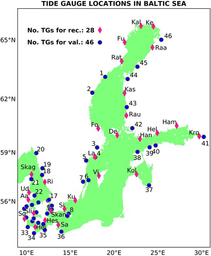
For the training of the reconstruction algorithm, we use as proxy data for the period 01/01/2019–31/12/2019 outputs from the operational model of the SMHI (Swedish Meteorological and Hydrological Institute) BAL MFC-NEMO (product ref. 3.4.1). These data are referred to as the ‘Baltic Sea Physics Analysis and Forecast’ product of the CMEMS Baltic Monitoring and Forecasting Centre (BAL MFC). We will use the abbreviation ‘ANL’ for this data set further on in the text. We define the global state vector x as the data set, which contains hourly maps of SSH over the entire Baltic Sea. The measurement vector y is assumed to represent the observations from the coastal stations (see ). In our training step, we use for the measurement vector proxy measurements from the model and postulate the following relationship. (3.4.1) $y = H x,$ (3.4.1) where H is called the linear measurement operator. These proxy measurements are without temporal gaps or measurement errors. In the following, it is assumed that the state vector $x$ and the measurement vector $y$ have their temporal mean removed, thus, they describe the departures of sea level $x^{'}$ from a reference sea level ${\bar{x}}_{t}$ , which is considered as the temporal mean over the training period (01 January 2019–31 December 2019).

The task for the training is to find a linear reconstruction matrix A, which applied to the data in the positions of observations (gauge stations), could reconstruct the Sea Level Anomaly (SLA) over the entire area. Such reconstruction would be optimal if the cost function (3.4.2) $J (A) = \sum_{j = 1}^{q} x (t_{j}) - A y (t_{j})^{2}$ (3.4.2) is minimum, where q is the number of hourly maps used for the training. This would ensure that the reconstruction error is as small as possible. Schulz-Stellenfleth and Stanev (Citation2010) showed that J(A) is minimum if A is the Kalman gain matrix (3.4.3) $A = P H^{T} (H P H^{T} + R)^{- 1}$ (3.4.3)

where P is the background covariance matrix for the state x and R is the observation error matrix for the measurements y. There are some limitations to the method and we refer to the work of Janjić et al. (Citation2018) for more details on how to overcome them. In the present work, we use for R a diagonal matrix with a constant observation error of 1 cm. For P we use empirical orthogonal functions (EOFs; Preisendorfer and Mobley Citation1988) of the entire Baltic Sea estimated during the training period. A well-known advantage of the described design is that only a few EOFs are needed to give a good approximation of the covariance information in P, which significantly reduces the dimension of the reconstruction problem and makes the calculation of A efficient. In order to catch the long-time variability over decades, which for the Baltic Sea represents a marginal part of the total variance, we build P from the leading 30 EOFs, which describe more than 99.5% of the total variance. An analyses of these EOFs can be found in the appendix of the study (Appendix A; Analyses of proxy data used for the training of the reconstruction method.).

illustrates the validation of the training, quantified as the mapped root mean square error (RMSE) of the reconstruction for the training period, (3.4.4) $RMS E_{i} = \sqrt{\frac{1}{q} \sum_{j = 1}^{q} {(x_{i} (t_{j}) - A_{i} y (t_{j}))}^{2}}$ (3.4.4) where i denotes the individual position. Because the design of the training provides perfect observations for the method (no measurement errors), the errors in the reconstruction emerge from the missing linear correlation between the observed and the remote positions in the training data set. It is not surprising that the lowest errors are found along the coast and close to the position of gauge stations because these regions can be expected to have higher linear correlation with the data in the gauge stations. RMSEs in the region of the Skagerrak, Kattegat, Great Belt, Sound and the eastern part of the Gulf of Finland are in general higher, due to limitations of the reconstruction approach to reproduce the complex dynamics in these regions. Higher errors in the Bornholm basin and along the Polish coast are due to the lack of observations there (compare ).

Figure 3.4.2. The performance of the reconstruction method expressed as the RMSE difference between the global state $x$ and its reconstruction during the training period. Product used: ref. 3.4.1 (ANL).

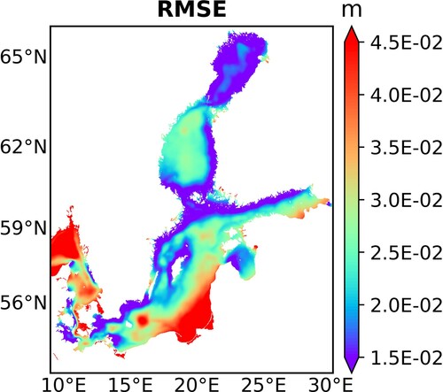
The application of the Kalman filter approach described above, as well as the application of generative adversarial networks to reconstructing basin wide sea level in the North Sea has been addressed in detail by Zhang et al. (Citation2020). Advantages and limitation of the method are described in that study, therefore, we will not repeat here the exercise of these authors but give a brief overview. One message of their study was that substituting the proxy (model gauges) by data from real observations decreases the quality of the reconstruction skill. One reason for this is that the correlation patterns of the training data set not necessarily mirror correlations between real observations, which limits the reproducibility of the real observations in the reconstruction. The decomposition of correlation patterns into EOFs is only partially able to overcome this limitation. In general, the method is better able to deal with missing or underestimated correlations than overestimated or spurious correlations, with smooth training data dominated by a few periodic signals with a limited number of frequencies (e.g. tides) giving more vulnerable EOFs. In the present work, we will propose an extended approach, which could be considered as an enhancement of model data by real observations. We build our approach on strengthening the synergy between observations and numerical simulations. Expressed in another way, the method can be considered as a posteriory ‘assimilation’ of coastal data. The advantage over the method described in Zhang et al. (Citation2020) is that, instead of reconstructing the observations, we reconstruct the misfit between the observations and the numerical simulations, which we believe to have a better chance to be representable by the correlation patterns of the training data than the observations themselves.

The reconstruction period (1993–2020), which we target is longer than the training period, that is the model solution and observations are independent data from the ones used in the training. We use the same reconstruction matrix $A$ as derived during the training phase. However, as mentioned above, instead of using proxy measurements, as we did during the training phase, we will use in the following real measurements from the data set TGD-P28. We will denote the real observation as $y_{o}$ . The subscript ‘o’ stands for ‘observations’. Our basic assumption is that the background covariance matrix P is representative not only for the training period, but also for the validation period. The algorithm uses SSH fields, not SLA, from numerical simulations as a first guess and calculates updated fields based on real measurements. Simulation data for the year 2020 is derived from the same CMEMS product (ANL, product ref. 3.4.1) as the training data set. The period from 1993 to 2018 is available from the ‘Baltic Sea Physics Reanalysis’ CMEMS product (product ref. 3.4.2), see Hordoir et al. (Citation2015) and Pemberton et al. (Citation2017), for which we will use the abbreviation ‘REA’, in the following. For the longer reconstruction period, the linear measurement operator H and the reconstruction matrix A have to be considered as time dependent because continuous observations over the whole validation period are not available from all gauges. Accordingly, the reconstructed state ( $x_{r}$ ) for the time $t_{j}$ (hourly maps during the reconstruction) is presented as (3.4.5) $x_{r} (t_{j}) = x (t_{j}) + A (t_{j}) [y_{o} (t_{j}) - H (t_{j}) x (t_{j})]$ (3.4.5) This equation can be regarded as correction of model estimate $x (t_{j})$ by the second term on the right-hand side. In the case of using proxy data from the model instead of real observations $y_{o} (t_{j}) - H (t_{j}) x (t_{j}) = 0$ , the solution is $x (t_{j}) .$ The deviation between coastal observations and model data on the coast tends to correct $x (t_{j})$ basin wide. As far as biases are concerned, because of the different training and reconstructing periods, they are in the range of few millimeters, which is far below the achievable accuracy for the reconstruction method (see ). Therefore, they are not considered. Quantifying the effect of possible biases in additional experiments (not presented here) showed little to no gain in the reconstruction’s performance. We will use in the following text the abbreviation ‘REC’ for the reconstructed state estimates (product ref. 3.4.5).

illustrates the availability of gauge measurements in the TGD-P28 data set and their consistency with the REA and ANL data from the Baltic Sea CMEMS numerical simulations. Basic SSH events during the period covered by REA (1993–2018) are coherent in the two data sets and no obvious bias is observed for this period. For the rest of the time (2019–2020), which is covert by the ANL data, we find a positive bias in comparison to the TGD-P28 data. To understand the reason for this, we performed experiments with an independent model that included the same region. These experiments showed a comparable bias in SSH after 2018. Subsequent analyses of the forcing data for the lateral open boundaries (CMEMS) and the surface (ERA5, product ref. 3.4.4) showed no suspicious changes in the spatial patterns or absolute values between 2017 and 2019, so we suspect that noise accumulation is the cause of the bias. However, a more detailed investigation in the future may prove otherwise. Another problem is that in the transition area between the North Sea and Baltic Sea, continuous observations are available only after 2013. Because of these two reasons, it is expected that the performance of the reconstruction will be inferior in that region for the period before 2013 and in the time after 2018.

Figure 3.4.3. Comparison between tide gauge observations (top) and numerical simulations (bottom) in the locations used for training (28 tide-gauge locations, compare ), but for the longer than training period. Products used: ref. 3.4.1 (ANL), ref. 3.4.2 (REA) and ref. 3.4.3 (TGD-P28).

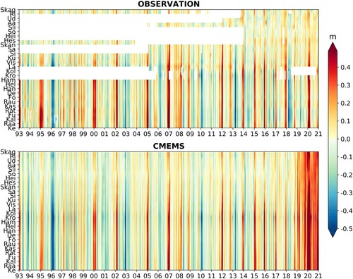
summarises for all data sets used during the training and application of the reconstruction algorithm the period covered, the intended use, and their abbreviation in the text. In addition, the corresponding product references are given in the table's caption where appropriate.

Table 3.4.1. Covered period and purpose for all data sets used during the training and application of the reconstruction algorithm. The abbreviation ‘ANL’ and ‘REA’ refer to the ‘Baltic Sea Physics Analysis and Forecast’ and ‘Baltic Sea Physics Reanalysis’ CMEMS products, respectively (product ref. 3.4.1 and ref. 3.4.2). ‘TGD-P28’ and ‘TGD-P46’ indicate the tide-gauge data sets including the 28 stations used for reconstruction and the 46 stations used for independent validation. Both data sets are derived from the ‘Baltic Sea – In Situ Near Real Time Observations’ CMEMS product (product ref. 3.4.3). ‘ERA5’ refers to the atmospheric data from the Fifth generation of ECMWF atmospheric reanalyses of the global climate product (product ref. 3.4.4) from the Copernicus Climate Change Service Climate Data Store (CDS). ‘REC’ stands for the SSH reconstruction based on Equation 3.4.5 (product ref. 3.4.5).

3.4.3. Results

The validation of the reconstruction is performed at the coastal station positions and takes into consideration the measurements, which are not used in the reconstruction. shows a comparison between the reconstructed sea-level signals and those retrieved from observation- and model-based data sets. In particular, we assess the reconstruction in terms of correlation with the observations (left), and skill compared to CMEMS simulations (right). The latter is defined as (3.4.6) $RMS E_{r} = \sqrt{\frac{1}{N} \sum_{j = 1}^{N} {[H_{j} x_{r} (t_{j}) - y_{o} (t_{j})]}^{2}}$ (3.4.6) (3.4.7) $RMS E_{c} = \sqrt{\frac{1}{N} \sum_{j = 1}^{N} {[H_{j} x (t_{j}) - y_{o} (t_{j})]}^{2}}$ (3.4.7) (3.4.8) $SKILL = 1 - \frac{RMS E_{r}}{RMS E_{c}}$ (3.4.8) where $RMS E_{r}$ and $RMS E_{c}$ are the errors obtained by comparing the observations with the reconstructed sea-level and CMEMS model outputs, respectively. N is the number of available observations during the investigated periods. Results are shown for two periods: 1993–2019 (top) and for 2020 (bottom). The first period is covered by the REA data set and the part of the ANL data (2019, product ref. 3.4.1) that was used for training. The second period is covered by the portion of the ANL data (2020) that is independent from the training. The diamond and circle symbols correspond to the gauge locations that were used (TGD-P28) or not used (TGD-P46) in the reconstruction, respectively. The general conclusion is that the correlation and the skill of reconstruction are good, except for the straits connecting the North and Baltic Seas. This is probably related to the limited ability of the reconstruction design to reproduce the dynamics in this region. We have already addressed this issue in the validation of the training period (see ). Another reason for the inferior performance is the lack of observations in the area. In general, the gaps in the time series of measurements during the period 1993–2019 (see ) affect the quality of the reconstructions. In contrast, if we consider a period when continuous in-situ records were available, the correlation between observations and reconstructions improves significantly (e.g. in 2020, (C)). Whereas we attribute the concurrent decrease of the skill for the region (compare (B) and (D)) to a better performance of the ANL simulation rather than to a lowered performance of the reconstruction. There are other regions, such as the Gulf of Riga, where the validation is rather poor in both periods (circle symbols in (B,D)). For this area, the data set of the only tide gauge station used for reconstruction, ‘Kolka’ (Kol), has significant gaps in both periods. However, high negative skills are found only for 2020 and at some stations in the transition zone between the North Sea and the Baltic Sea and the straits, where skills are generally low (see above). Further validation and statistics on the reconstructed data can be found in the appendix of the study (Appendix B; Extended validation and statistics of the reconstructed data).

Figure 3.4.4. Correlation against observations (left-hand side) and Skill against SMHI data (right-hand side) of the reconstructions for the periods 1993–2019 (top) and 2020 (bottom) at the 46 independent (circles) and 28 dependent (diamonds) tide gauge locations. Products used: ref. 3.4.1 (ANL), ref. 3.4.2 (REA), ref. 3.4.3 (TGD-P28, TGD-P46) and ref. 3.4.5 (REC).

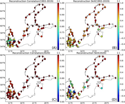
The panels in show SSH 99th percentiles obtained considering the data sets REC and TGD-P46, where colours of the circular symbols represent the 99th percentiles as seen in the tide gauge data. The basin-wide reconstruction agrees well at the coastal stations with the independent coastal observations. The results show that over the period 1993–2019, the SSH extreme values reach maximum in the easternmost part of the Bay of Finland, as well as in the northernmost part of the Bothnia Bay ((A)), which are even intensified in these areas in 2020 ((B,C)). In addition, the Swedish coast shows stronger-than-average values in 2020 ((B,C)).

Figure 3.4.5. Mean yearly 99% percentile of SSH for the period 1993–2019 (A), the year 2020 (B) and the anomalies of the values in 2020 from the values of the rest of the period (C). The coloured maps and dots show the values derived from the reconstructions (REC) and independent tide gauges (TGD-P46), respectively. Tide gauge locations with insufficient observations are not shown in the panels. Products used: ref. 3.4.3 (TGD-P46) and ref. 3.4.5 (REC).

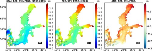
In the following, we address sea-level variations on interannual to longer time scales. Climate modes such as the NAO are known to be a major driver of sea level variability in this area and on these time scales. To further investigate the relationship between regional and global variability, we compare the reconstructed sea level anomaly over the period 1993–2020 with the NAO index at the regional scale during the winter season (December-January-February, DJF). As can be seen in (A), the correlation between the reconstructed sea level anomaly and the NAO index reaches values above 0.8 in the inner Baltic Sea, while lower values are observed in the transition area to the North Sea. Similar results are provided by the comparison between the NAO index and the independent tide gauge data (TGD-P46, circles in (A)) in the region, which generally supports the results obtained from the reconstruction. This regional change in the response to the NAO may be related to the complex dynamics in the region, which emerge from the interaction between the transport through the straits and the bathymetry (see e.g. Haid et al. Citation2020). Regions where the correlation coefficients derived from the tide gauge data and the values derived from the reconstruction differ are the Gulf of Riga and the Gulf of Finland. Here, the reconstruction slightly overestimates the correlation. The discrepancies along the southern coast and in the eastern part of the Gulf of Finland suggest that the spatial correlation patterns in this region may in fact be more complex than the reconstruction results suggest. In addition, we want to analyse the response of our reconstructed sea level anomaly to the NAO by evaluating the difference between the mean sea level anomaly at the southwestern opening of the Baltic Sea, the Arkona Basin, and the northern tip of the basin, the Bothnian Bay. Both regions are shown as green frames in the figure. The results of the reconstructed data (red solid line in (B)) show the agreement between the normalised reconstructed sea level differences and the NAO index for the winter season and emphasise the influence of the large-scale external wind conditions on the sea level variability in the Baltic Sea. This result is confirmed by comparing the climate index with the observed sea level records (black dashed line in (B)). The strong influence of the atmospheric patterns on the temporal evolution, shown in , indicates that the Baltic Sea can be considered as an almost perfect responder to the NAO, in line with the results of Andersson (Citation2002) and Passaro et al. (Citation2021).

Figure 3.4.6. Correlation coefficient of the reconstructed sea level anomaly (map) and tide gauge observation (coloured circles) with the North Atlantic Oscillation (NAO) index during winter season (DJF, December–January–February) for the period 1993–2020 (A). Time series of the normalised DJF NAO index and normalised mean SSH differences between the Bothnia Bay and Arkona Basin (B) from REC (red solid line) and from TGD-P46 observations (black dashed line). Observations in the northern box (‘Botnian Bay’) are represent by the measurements derived from the stations: Kemi, KalixStoron, Furuogrund, Ratan, Skagsudde, Vaasa, Pietarsaari, Raahe and Oulu; Observations in the southern box (‘Arkona Basin’) are represented by the measurements derived from the stations: Simrishamn, Skanor, Rodvig, Hesnaes, Sassnitz, Koserow and Tejn. Products used: ref. 3.4.3 (TGD-P46), ref. 3.4.4 (ERA5) and ref. 3.4.5 (REC).

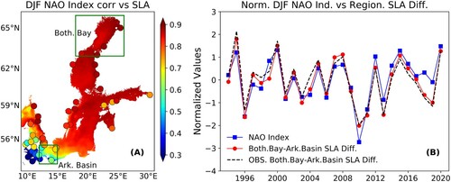
3.4.4. Conclusions

Multi-year (1993–2020) sea level variability in the Baltic Sea is reconstructed using a combination of tide gauge observations (TGD-P28) and model-based data (ANL and REA). The results have shown that the dynamic model simulation (ANL) are able to provide a reliable basis for describing the spatial sea level correlation patterns, which are needed as an initial assumption for the reconstruction process. In addition, our study has demonstrated the ability of the algorithm to reconstruct sea level anomalies on different space and time scales.

Validation of the reconstruction algorithm with training data from the model simulation showed that it has limited ability to compensate for the unfortunate lack of tide gauge data along the Polish coast. Lower reconstruction performance is expected here and in the Bornholm Basin region, but could not be evaluated due to lack of other validation options. In addition, reconstruction performance in the transition zone between the North Sea and the Baltic Sea was shown to decrease during periods of lower local data coverage. The low correlation in this area with observations in the rest of the basin may also indicate that the region is governed by complex dynamics (see also Zhang et al. Citation2016; Stanev et al. Citation2018; Haid et al. Citation2020).

Our results showed that the extreme sea level anomalies in 2020 reached unusually strong values compared to the 1993–2019 baseline, especially in the northernmost and easternmost parts of the basin. Moreover, the strong relationship between sea level change in the Baltic Sea and the NAO was quantified.

Large parts of the Baltic Sea coast are endangered by storm surges. Due to their potential to cause devastating damages, the precise prediction of form, timing and duration of storm surges has a high societal impact. In order to achieve this high forecast skill, state-of-the-art model systems rely on the practices of observation data assimilation. However, the temporal availability of altimeter observations is often not high enough to catch storm surges with duration of hours to days. The results obtained in this study demonstrated that: reconstruction methods offer comprehensive high-resolution estimates (space and time) of sea level variability in the Baltic Sea based on tide gauge observations at high temporal resolution (e.g. hourly). This approach can be a valuable extension of existing observational capabilities from remote sensing (Passaro et al. Citation2021), as it can be used to fill temporal gaps typical of any observing system and track the temporal evolution of sea level patterns at high resolution. At the same time, the method consumes only a fraction of the computational resources required by an assimilative model with comparable temporal and spatial resolution.

Acknowledgments

The production of the results presented in this study used computational resources of the MISTRAL cluster system of the Deutsches Klimarechenzentrum (DKRZ) granted by its Scientific Steering Committee (WLA) under project ID bu1213.

Section 3.5. Wave climate extremes in the Mediterranean Sea obtained from a wave reanalysis for the period 1993–2020

Authors: Anna Zacharioudaki, Michalis Ravdas, Gerasimos Korres

Statement of main outcome: Climate change can alter the extreme wave climate of the Mediterranean Sea and consequently modify the risk posed on maritime structures and coastal environments. The annual 99th percentile of Significant Wave Height (SWH) – a measure of extremes – has increased almost everywhere in the basin during the last 28 years at a maximum rate of 0.026 m/year. The most significant upward trends were found in the south-eastern Levantine and eastern Alboran Seas, followed by the Adriatic Sea and contained areas of the Tyrrhenian. The same areas were found to be prone in terms of changes in wave storm characteristics such as frequency, intensity and duration, embedding statistically significant positive trends over this period. Additional regions with consistent positive trends include the Catalan coast and its offshore and the coast of Valencia, around the western end of the island of Crete and the north-east Aegean. Negative trends are not uncommon in wave storm intensity and duration, yet not statistically significant. No negative trends have been identified in wave storm frequency. A large inter-annual variability is associated with the results. These findings are valuable to engineers and stakeholders towards alleviating any additional risk posed on the marine sector and coastal activities by climate change.

Data use:

Table

3.5.1. Introduction

The study of extreme wave climate and wave storms is very important and of great relevance to engineering practice. It is crucial for the design and safety control of marine vessels, of offshore and coastal structures (e.g. oil/gas platforms, aquaculture, wind and wave farms), as well as coastal infrastructure (e.g. ports, roads, touristic facilities) (e.g. Gouldby et al. Citation2014). They are responsible for coastal flooding and affect coastal erosion (e.g. Harley et al. Citation2017). Climate change results in long-term changes of the extreme wave climate (e.g. Lobeto et al. Citation2021). Thus, for long-term sustainable planning of marine and coastal activities, the understanding of inter-annual variability and of climatic trends is also very important. Historic and future wave climate changes may require adaptation measures. For example, an increase in the frequency, intensity, and/or duration of wave storm events over a certain region may require enhanced protection from coastal hazards, re-direction of shipping routes or re-enforcement of marine structures (e.g. Bitner-Gregersen et al. Citation2013; Kirezci et al. Citation2020). It may increase downtime of operations at sea and it might require advanced systems of alert (e.g. Reeve et al. Citation2011; Camus et al. Citation2019; Spinoni et al. Citation2020).

Several studies have examined the extreme wave climate of the Mediterranean Sea (e.g. Zacharioudaki et al. Citation2015; Sartini et al. Citation2017; Morales-Márquez et al. Citation2020; De Leo et al. 2020) with a number of them focusing on wave storm characteristics (e.g. Zacharioudaki et al. Citation2015; Besio et al. Citation2017; Amarouche and Akpinar Citation2021; Martzikos et al. Citation2021). The vast majority of these recent studies have relied on wave hindcasts that cover a long time period and have a high resolution. Nevertheless, coarser resolution global studies that use satellite observations (e.g. Young and Ribal Citation2019) or local studies that use buoy measurements (e.g. Martzikos et al. Citation2021) can be found. However, the time frequency of the satellite sampling is considered inadequate for well capturing storm peaks in the highly variable environment of the Mediterranean Sea whereas the spatial sampling of the in-situ observations is not appropriate for studying medium to large-scale wave climate. In addition, data inhomogeneities and gaps are often encountered in observational datasets. As a result, in-situ and satellite observations are mostly used to calibrate and validate the wave models.

In this paper, we study the extreme wave climate of the Mediterranean Sea focusing on wave storm characteristics such as wave storm frequency, intensity and duration. The long-term average statistics, climatic trends and inter-annual variability are examined. The focus is on the spatiotemporal distribution of wave extremes rather than the atmospheric conditions producing them (e.g. Sartini et al. Citation2017; Morales-Márquez et al. Citation2020; Amarouche et al. Citation2021). To this aim, we use a 28-year high resolution wave reanalysis, forced by the ERA5 reanalysis winds, and a peaks over threshold (POT) approach to indentify individual wave storm events. It is well known that the quality of a wave hindcast/reanalysis largely depends on the quality of the reanalysis wind forcing fields, which are continually improving. ERA5 is the most recent, publicly available, state-of-the-art global wind reanalysis dataset that has reached a time and space resolution that is adequately high so as to enable a proper assessment of the wave climate extremes in the highly variable environment of the Mediterranean Sea. In addition, the spatial resolution of the wave model, which is the highest used in similar studies involving the full Mediterranean Sea, is able to adequately resolve the fine bathymetric features in the basin caused by the presence of numerous islands, semi-enclosed sub-basins and bays. The assimilation of altimeter SWH, the consideration of wave-current interaction through the input of reanalysis surface currents along with the account of Atlantic swell through nesting to an Atlantic Ocean model are additional characteristics of the wave reanalysis used in this study that are expected to increase the accuracy of the computed extreme wave climate statistics.

3.5.2. Method

The wave reanalysis delivered by the Mediterranean Monitoring and Forecasting Centre (Med-MFC, product 3.5.1) provides hourly instantaneous fields of SWH at 0.041° horizontal resolution covering the Mediterranean Sea and extending up to −18.125°E into the Atlantic Ocean. It is based on the latest version of the state-of-the-art WAM wave model (WAMDI Group Citation1988; Komen et al. Citation1994). It is run in shallow water mode and is extensively tuned for the Mediterranean Sea. It is forced by hourly ERA5 reanalysis winds at about 30 km resolution. It inputs Med-MFC daily averaged surface currents to account for wave-current interaction, it is nested to a coarser resolution (1/6°) Atlantic model to properly account for swell passing in the Mediterranean Sea through the Strait of Gibraltar and assimilates all along-track satellite SWH observations available since 1993 (data are scarce before this year). It is noted that CMEMS has adopted year 1993 as the starting year for its reanalysis products so as to cover the period over which adequate inter-calibrated satellite observations exist for data assimilation.

A detailed description of the system can be found in the Product User Manual (PUM) and Quality Information Document (QUID) available in the CMEMS webpage (see product table). In the latter document, the product is thoroughly validated against in-situ and satellite data, products 3.5.2, 3.5.3 and 3.5.4, 3.5.5 respectively. In this work, a summary of the results is provided. In addition, yearly values of the agreement between collocated reanalysis and observed 99th percentile SWH will be presented for in-situ and satellite data respectively for the period 1993–2018. Observations from 53 wave buoys and 8 satellite altimetry missions have been used to perform the inter-comparisons. All the details of this procedure can be found in the QUID.

Different methodologies exist to isolate wave storms from a time-series of wave data (e.g. Besio et al. Citation2017; Amarouche and Akpinar Citation2021). Here, the methodology of Weisse and Günther (Citation2007), modified by Zacharioudaki et al. (Citation2015), is applied. In particular, the pointwise long-term 1993–2020 99th percentile SWH ((a)) is used as a threshold to determine severe wave conditions, referred to as wave storms. It is noted that there is not a largely accepted method for the selection of the threshold value (Ciavola and Coco Citation2017; Harley Citation2017). Values between the 90th and 99th percentile SWH are often encountered in the literature (e.g. Masselink et al. Citation2014; De Leo et al. Citation2020). In general, a high threshold is a valid choice when the data sample is sufficiently large and when the focus is on the most extreme events. Having set the threshold, the number of wave storm events is defined as the number of independent events that exceed this threshold. To assure the independency of the events, a spacing of 72 h between them has been adopted (e.g. Debernard and Røed Citation2008; Meucci et al. Citation2018). The intensity of each wave storm is defined as the difference between the maximum SWH that occurred during the storm and the local 99th percentile threshold. Finally, the wave storm duration is the time the storm’s SWH remained above the threshold. Based on annual values over the period 1993–2020, maps of average climate statistics and trends of the aforementioned quantities are obtained. Trends are computed using the non-parametric Sen's slope estimator for robust linear regression and are tested for statistical significance using the non-parametric Mann-Kendall test at the 5% significance level (i.e. p-value ≤ 0.05). These estimators are much less sensitive to outliers and skewed distributions compared to simple linear regression methods.

In addition to the long-term pointwise approach, described above, the inter-annual variability of the aforementioned quantities were investigated for a number of Mediterranean sub-regions giving us the possibility to identify sub-trends present within the 28-year period. In this case, the hourly modelled SWH was averaged over pre-defined sub-regions. The resulting regionally averaged time-series was then used to apply the methodology outlined in the previous paragraph.

3.5.3. Results and discussion

Overall, the significant wave height is accurately simulated by the model (QUID, product 3.5.2). Considering the Mediterranean Sea as a whole, the typical difference with in-situ and satellite observations (RMSE) is 0.23 ± 0.012 m (mean of yearly values ± standard deviation) and 0.24 ± 0.01 m respectively, the BIAS is −0.06 ± 0.022 m and −0.05 ± 0.011 m, the Scatter Index (SI) is 0.27 ± 0.015 and 0.17 ± 0.006 whilst the Correlation Coefficient (R) is 0.95 ± 0.001 and 0.96 ± 0.004 respectively. Spatially, the model performs optimally at offshore wave buoy locations and well-exposed Mediterranean sub-regions. Within enclosed basins and near the coast, unresolved topography by the wind and wave models and fetch limitations cause the wave model performance to deteriorate. To put the above results into context, the model skill of this study is compared to the high resolution study of Amarouche and Akpinar (Citation2021). Specifically, they used a SWAN wave model hindcast (Amarouche et al. Citation2019) at an horizontal resolution of 0.033°, forced by reanalysis winds at a resolution similar to that of ERA5, to study the storm wave climate and trends in the Western Mediterranean Sea. Their model skill was evaluated against in-situ observations resulting in an average SI of 0.3 and an average R of 0.93 for their full domain. Qualification metrics at individual buoy locations indicate that our reanalysis performs better at all common offshore locations used. In the nearshore, the two studies produce very similar statistics with the study of Amarouche and Akpinar (Citation2021) occasionally having a small advantage over our study. This is attributed to the higher resolution of their wave hindcast that better resolves the coast.

Focusing on the extremes, shows a very good agreement between reanalysis and first-guess 99th percentile SWH and collocated wave buoy and satellite observations respectively, merged over the Mediterranean Sea. The depicted differences do not exceed 0.3 m with the model mostly underestimating extreme wave heights. A higher model underestimation appears to occur in the period 1993–2000, mostly for the model-buoy comparison.

Figure 3.5.1. Yearly values of collocated reanalysis (product 3.5.1) and observed 99th percentile of SWH computed by merging wave buoy (left panel; products 3.5.2, 3.5.3) and satellite (right panel; products 3.5.4, 3.5.5) observations respectively in the Mediterranean Sea.

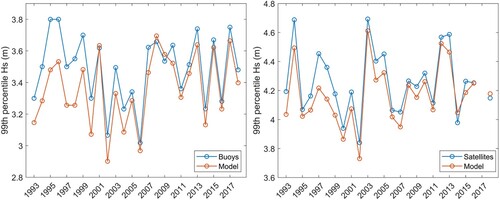
The 1993–2020 long-term 99th percentile SWH (hereafter referred to as threshold) and the climatic averages of the annual wave storm characteristics are shown in the left panels of . The 99th percentile SWH ((a)) is in alignment with previous studies (e.g. Sartini et al. Citation2017; Álvarez Fanjul et al. Citation2019; Morales-Márquez et al. Citation2020) where the reader may also find information on the atmospheric drivers related to the observed patterns. The average annual number of events exceeding the threshold ((b)) is 4–7 in most of the Mediterranean Sea. The highest number of wave storms (9–13) predominantly occur within regions that are characterised by a mild wave climate. Regions which are characterised by a stronger extreme wave climate and are additionally affected with a relatively high frequency of wave storms occur west of the island of Corsica (8–9 events) as well as offshore from the Catalan coast, in the Strait of Sicily and northern Ionian Sea (6–8 events). Martzikos et al. (Citation2021) and Amarouche and Akpinar (Citation2021) used lower thresholds and different methods for wave storm analysis and computed values of 10–14 at coastal locations and 10–16 over the western Mediterranean Sea respectively. The average annual wave storm intensities ((c)) have a range of 0.03–1.4 m. In general, high intensities are found over areas of high thresholds ((a)). An obvious exception is observed seawards from the Gulf of Lion, where the maximum intensities (1.2–1.4 m) are shifted southwards relative to the maximum thresholds, below about 42°N. Enhanced intensities (≈ 1 m) in relation to the threshold are observed in a number of regions including the area east of the Strait of Gibraltar, along the coast of Valencia, Liguria and southern Italy, south of Crete and in the eastern Levantine. The average annual wave storm duration ((d)) has a range of 8–27 h. Most of the aforementioned regions, showing enhanced intensities relative to the threshold, also appear to have high wave storm durations (except Liguria). The results on wave storm intensity and duration fall in line with those in Martzikos et al. (Citation2021) whilst similar durations are stated by Lionello et al. (Citation2006) in relation to Mediterranean cyclones. On the other hand, Zacharioudaki et al. (Citation2015) report higher values of wave storm intensities and durations in the Hellenic Seas which might be because their wave model was found to overestimate wave extremes.

Figure 3.5.2. (a) POT threshold: 1993–2020 long-term 99th percentile of SWH (m) and 1993–2020 average of (b) annual number of events exceeding the 99th percentile, (c) their average intensity (m) and (d) their average duration (hours); (e) 1993–2020 trends of the annual 99th percentile SWH, (f) the annual number of events exceeding the long-term 1993–2020 99th percentile, (g) their average intensity and (h) their average duration. Areas of statistically significant trends at the 5% significance level are within grey contours. The numbers shown in plot (a) denote regions and are used in .

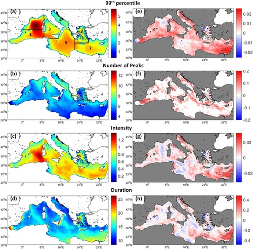
The 1993–2020 trends of the annual values of the 99th percentile SWH are shown in (e). The annual 99th percentile SWH shows widespread positive trends over the period 1993–2020. The trend slope reaches values up to 0.026 m/year with maximum values over the south-eastern Levantine Sea, followed by the eastern Alboran Sea. High values are also found over the south-western Mediterranean Sea between 5° W and 12° W, in the Adriatic Sea, and in other parts of the Levantine. Statistically significant trends (within grey contours in (e–,h)) are also found within these regions. These trends are spatially extended in the eastern Alboran Sea, between Corsica and Italy, along the western Adriatic, and over the eastern Levantine basin. Negative trends in the north-west Aegean Sea, around the Strait of Gibraltar, in the eastern part of the Gulf of Lion moving offshore towards the southeast, and in a small part of the western Ionian do not exceed −0.018 m/year and are not statistically significant. Comparison with previous studies revealed the sensitivity of trend estimates on the chosen percentile and on the underlying long-term time-period and/or short-term sub-annual period (e.g. only winters) selected for the analysis. Young and Ribal (Citation2019) also found mostly positive trends at similar rates in the Mediterranean Sea over the period 1985–2018. Also, trend estimates of the winter annual mean SWH (not shown) are in very good agreement with those presented in Timmermans et al. (Citation2020) when using the same period. Nevertheless, Morales-Márquez et al. (Citation2020) found extreme waves trends that are predominantly negative in the Mediterranean Sea for the period 1979–2009. Similarities and differences are found between our results and those of De Leo et al. (Citation2020) produced for the period 1979–2018. As mentioned in the introduction, this study is mostly interested on the wave climate rather than the forcing wind statistics. Nevertheless, it is worth noticing that an equivalent analysis on the forcing wind speeds (U10) produced 99th percentile U10 trends (not shown) that are in very good alignment with those shown in (e). The agreement is both on the spatial pattern of trend values and on their statistical significance. In the case of U10, maximum positive trends of statistical significance, found in the south-eastern Levantine, the Alboran Sea and the Adriatic Sea, reach values of about 0.05–0.06 m/s/year. Also, the statistically significant positive trends are more spatially extended in the case of U10 in relation to the area covered in the case of SWH.

(f–h) shows the 1993–2020 trends of the wave storm characteristics whose climatic averages were shown in the corresponding left panels of . Regarding the annual number of wave storm events, this is mostly unchanged or has increased within the examined period ((f)). Statistically significant positive slopes are few and largely localised. The most spatially extended region of statistically significant increase is the eastern Alboran Sea, i.e. the area of maximum slope at 0.2 events/year. On the other hand, Cavicchia et al. (Citation2014) and González-Alemán et al. (Citation2019), focusing on Medicanes, found that their frequency is projected to decrease in future climate change scenarios whilst a moderate increase is projected for their intensity. In , wave storm intensity and duration have maximum positive slopes in the eastern Levantine Sea with values of 0.032 m/year ((g)) and 0.482 h/year ((h)) respectively. These are statistically significant. Somewhat smaller but significant rates are also observed in the western part of the Levantine basin. The Adriatic Sea, the area between Corsica and mainland Italy, and the west coast of Tunisia also show statistically significant positive trends. Intensity alone is increasing significantly (≈ 0.03 m/year) along the coast of Valencia while duration does so along the south Tyrrhenian exit. In general, statistically significant positive trends in wave storm characteristics do translate to significant trends in the overall extreme wave climate ((e)). Also, there are regions where all wave storm characteristics do show positive trends, even if not statistically significant, such as the Catalan coast and offshore, over the southern extremity of the Tyrrhenian Sea, a considerable part of the Adriatic Sea, around the western end of Crete island, in the north-east Aegean as well as in parts of the Levantine Sea. Negative trends in intensity and duration reach −0.024 m/year and −0.43 h/year respectively and are not statistically significant. The greatest decrease in wave storm severity is found in the north-east Aegean Sea. Widespread decrease is also seen west of Corsica and Sardinia in the offshore, in the western Ionian Sea and Sicily Strait, and east of the island of Crete. Despite using different methodologies, the wave storm intensity trend directions obtained herein have a lot of similarities with those obtained in Amarouche and Akpinar (Citation2021) for the western Mediterranean Sea for the period 1979–2019; the most apparent discrepancy is found in the Tyrrhenian Sea. Comparing the results in (f–h) to equivalent results obtained for U10 (not shown), a correspondence between U10 and SWH trends is mostly observed, corroborating the causal relationship of wind speed and SWH. In the case of U10, the annual number of storm events shows more widespread positive trends that are statistically significant over more regions compared to those found for SWH. In terms of intensity and duration, a similar spatial pattern of trends is found for the two variables. The Levantine Sea shows the most significant positive trends reaching values of 0.06 m/s/year and 0.3 h/year in U10 storm intensity and duration respectively.

shows the inter-annual variation of the wave storm characteristics after averaging SWH over the regions defined in (a). The sub-regions generally show large inter-annual variability in wave storm characteristics (also the case for Regions 1, 6, not shown). Strong positive trends in the annual 99th percentile SWH (not shown) are found for the Tyrrhenian and Levantine Seas (p-value ≈ 1) and for the Adriatic (p-value = 0.03). In the Tyrrhenian, an enhanced positive trend in wave storm duration is found whilst in the Levantine both intensity and duration show statistically significant positive trends. In the Adriatic Sea, it is the frequency of occurrence and the duration of the wave storms that show statistically significant increases. For the north west Mediterranean and the Ionian Sea, although the 1993–2020 trend slopes are not statistically significant, statistically significant sub-trends are encountered. In both regions, a turning point occurs around year 2000. Thus, in the former region, a significant positive trend is found in the number of peaks since year 2000 accompanied by a significant decrease in wave storm intensity. In the latter region, significant negative sub-trends are found in the earlier years in wave storm intensity and duration that become significantly positive in the period 1998–2017.

Figure 3.5.3. 1993–2020 inter-annual variability of the annual number of events exceeding the long-term 1993–2020 99th percentile SWH, their average intensity and duration, computed for the sub-regions of the Mediterranean Sea defined in (a) (relevant numbers in (a) are shown in front of the name of the sub-region on the right side of the panels in ).

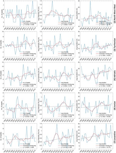
3.5.4. Conclusions

The present study assessed the extreme wave climate of the Mediterranean Sea over the last 28 years, using a high resolution wave reanalysis forced by the ERA5 high resolution global reanalysis. Adopting a Peaks over Threshold approach, the study focused on the characteristics of the most extreme wave storms and on their climatic trends and inter-annual variability.

It was found that the annual 99th percentile SWH, a measure of the overall extreme wave conditions of an area, exhibits an increasing trend almost over the entire Mediterranean Sea. The maximum trend slopes (0.026 m/year), significant at the 5% significance level, occur in the east Levantine Sea and eastern Alboran Sea. In the former basin, the increase could be linked to a statistically significant increase in wave storm intensity (up to 0.032 m/year) and duration (up to 0.48 h/year), also present in other, more localised, areas of the basin. In the latter, it is the wave storm frequency that increased significantly (up to 0.2 events/year) in the last 28 years. The Adriatic Sea also exhibits, spatially extended, statistically significant positive slopes in the 99th percentile SWH, wave storm intensity and duration. The Tyrrhenian Sea, mainly its north and south ends, is also active in terms of significant increases in wave extremes. In general, wave storm frequency exhibited only zero or positive slopes but mostly statistically insignificant. Negative slopes were computed for wave storm intensity and duration but, again, of no statistical significance. Nevertheless, considering the northwest Mediterranean Sea as a whole, statistically significant negative trends in wave storm intensity were computed for the period since year 2000. The same year was also found to be a turning point between negative and positive trends of statistical significance for the wave storminess of the Ionian Sea. Generally, the inter-annual variability of the wave storm characteristics was found to be large.

The estimated changes in the extreme wave regime of the basin are important for the identification of areas that are more vulnerable to hazards linked to climate change and a valuable tool for engineers and stakeholders in terms of sustainable development of maritime activities. For example, it is along the eastern Spanish coast – where a positive slope in all wave storm characteristics is computed in this study and is statistically significant in terms of wave storm intensity at the coast of Valencia – that Storm Gloria, a record breaking storm in terms of SWH, occurred in January of 2020, causing great damage to the coast (Amores et al. Citation2020; de Alfonso et al. Citation2021; Alvarez-Fanjul et al., Citation2022). By extrapolation, there is a higher probability of occurrence of similar events over regions where a significant increase in wave storminess is estimated over the last 28 years. This, in combination with a broader evaluation of a region in terms of topography, socio-economic activity, sea-level changes etc, can help prescribe a vulnerability index, and, in accordance, the degree and type of intervention in terms of protective measures.

Section 3.6. Surface warming of the Tyrrhenian Sea and local extreme events over the last four decades

Authors: Naomi Krauzig, Enrico Zambianchi, Pierpaolo Falco, Pieter Groenemeijer, Karina von Schuckmann

Statement of main outcome: The Tyrrhenian Sea, one of the most potentially vulnerable sub-basins of the Mediterranean Sea, experienced continuous warming since the early 1980s with increasing occurrences of extreme warm surface conditions during recent years. These conditions enhance the likelihood of ecological impacts with economic consequences, especially during strong marine heatwaves in summer. Our overview provides new insight into seasonal changes and anomalies of the surface warming in the Tyrrhenian Sea, addressing crucial information for aquaculture management and marine conservation efforts. Additionally, this section presents for the first time reported extreme weather events that led to damages, injuries, or fatalities in the highly populated area surrounding the Tyrrhenian Sea. These events are already among the most serious challenges to society in coping with a changing climate. Systematic monitoring of the amplifying socio-economic and environmental impacts is therefore critical for risk assessments and the development of feasible adaptation strategies.

Products used:

Table

3.6.1. Introduction

The Intergovernmental Panel on Climate Change (IPCC) fifth Assessment Report (AR5) of 2014 already affirmed that our climate and its extremes are changing and that associated projected risks will continue to increase as global mean temperature rises (IPCC AR5 Citation2014). The latest IPCC Special Reports concerning the impacts of climate change on land (IPCC SRCCL Citation2019) and on the ocean and cryosphere (IPCC SROCC Citation2020) emphasise the severity of impacts from extreme events for human systems and ecosystems.

While IPCC AR5 provided evidence that the surface and upper ocean has warmed significantly since 1970 (IPCC AR5 Citation2014), SROCC and the newest Assessment Report (AR6) confirmed that the occurrence of extreme ocean temperatures poses an even higher risk than long-term warming (IPCC SROCC Citation2020; IPCC AR6 Citation2021). Events of warm temperature anomalies in the ocean prompt substantial disruptions to marine ecosystems and their services (Mills et al. Citation2013; Rivett et al. Citation2014; Hobday et al. Citation2016; Frölicher and Laufkötter Citation2018; Smale et al. Citation2019). Known as marine heatwaves (MHW, Hobday et al. Citation2016), these extreme events describe abrupt but prolonged periods of high sea surface temperatures (SSTs) that have the potential to extend, or even intensify deeper in the water column (e.g. Schaeffer and Roughan Citation2017; Bensoussan et al. Citation2019; Elzahaby and Schaeffer Citation2019; Darmaraki et al. Citation2019; see also De Boisseson et al. in Section 3.3) through processes like detrainment and subduction (Holbrook et al. Citation2020; Elzahaby et al. Citation2021), the action of downwelling favourable winds (Schaeffer and Roughan, 2107) or possibly by the classically investigated mechanisms of internal wave- and tide- induced mixing (e.g. Wunsch and Ferrari Citation2004).

MHWs have become more frequent, extensive and intense (Frölicher and Laufkötter Citation2018; Oliver et al. Citation2018) with detrimental impacts on organism distributions, ecosystem functions and fisheries productivity with cascading impacts on economies and societies (e.g. Oliver et al. Citation2018; Darmaraki et al. Citation2019; IPCC SROCC Citation2020). Whereas MHWs have received considerable attention in recent years, much less has been documented on their cold equivalent, known as marine cold-spells (MCSs, Schlegel et al. Citation2017; Feng et al. Citation2020) that also have the potential to severely impact organisms and ecosystems (Lirman et al. Citation2011; Szekeres et al. Citation2016; Wakelin et al. Citation2021).

As in the ocean, extreme events in the atmosphere such as heatwaves, heavy precipitation and floods, droughts and storms have been shown to affect human societies and ecosystems in a fundamental manner (Parmesan et al. Citation2000; IPCC AR5 Citation2014; IPCC SRCCL Citation2019). The latest IPCC reports provide overwhelming evidence that several extreme weather events are already changing under global warming, increasing the risk of pervasive and in some cases irreversible impacts such as loss of life, damages to buildings, agricultural production and natural capital (IPCC SRCCL Citation2019).

Due to the intensification of extreme atmospheric and oceanic events (Hirabayashi et al. Citation2013; IPCC AR5 Citation2014; Kundzewicz et al. Citation2017; IPCC SRCCL Citation2019; IPCC AR6 Citation2021), relevant studies at global scale have increased significantly in the last few years. However, the impacts on ecosystems and human societies depend primarily on regional trends and the local manifestation of global-scale changes (IPCC SROCC Citation2020). In addition, science-based information and monitoring at regional and local scales is necessary for sufficient risk assessment and the development of feasible adaptation strategies (Cheng et al. Citation2021). Thus, in Mediterranean context, it is critical to focus on individual sub-basins, especially those with very high population density along their surrounding coasts. The target of our investigation, the Tyrrhenian basin, is the most populated semi-enclosed one (UNEP/MAP Citation2012) and therefore one of the most potentially vulnerable basins in the Mediterranean Sea (Smith et al. Citation2014). Furthermore, the Tyrrhenian Sea stands out because its response to global warming differs from that of the Mediterranean Sea as a whole (Krauzig et al. Citation2020) even though it interacts hydrologically and dynamically with the central Mediterranean in the south (Poulain and Zambianchi Citation2007; Rinaldi et al. Citation2010) and with the Ligurian Sea in the north (e.g. Astraldi and Gasparini Citation1994; Marullo et al. Citation1994; Vignudelli et al. Citation2000; Pisano et al. Citation2020). Even though the necessity of local studies has become evident, specific assessments of extreme atmospheric and oceanic events are still missing. To this end, our section provides insights into the prevalence of MHWs and MCSs in the Tyrrhenian Sea and serves as a constructive first step to understand the increasing risks of extreme weather events in the surrounding area.

3.6.2. Methodology

This study takes advantage of the longest freely available high-resolution satellite-derived L4 SST dataset from the Copernicus Marine Environment Monitoring Service (CMEMS product Ref. No. 3.6.1 and 3.6.2), as well as the fifth generation of ECMWF atmospheric reanalysis (ERA5 product Ref. No. 3.6.3) from the Copernicus Climate Change Service Climate Data Store in order to analyse them together with reports of extreme weather events from the European Severe Weather Database (ESWD product Ref. No. 3.6.4) over a period of nearly four decades (1982–2020).

The spatio-temporal variability of the mentioned SST and atmospheric data was studied by analysing the intra- and inter-annual geographical and climatological distributions of averages, anomalies and trends within the geographical boundaries of the Tyrrhenian Sea. If not indicated otherwise, all mentioned time series (daily, monthly, seasonal, yearly) were based on the spatial average of this area over the entire 39-year study period whereas the anomalies were computed against the 1982–2014 core climatology. Hot extremes were defined as the top 10% (90th percentile) of the daily SSTs and cold extremes as the daily SSTs at the bottom 10% (10th percentile).

Accordingly, following Hobday et al. (Citation2016) and Schlegel et al. (Citation2017), MHWs and MCSs were categorised as anomalous warm and cold events that last at least five days, with temperatures exceeding the seasonally varying threshold computed for each day based on the climatological period 1982–2014. Two events with a temporal gap of less than 2 days were treated as a single joint event. After the events were defined, a set of metrics was calculated including maximum and mean intensity (measured as anomalies relative to the climatological mean, in °C), duration (time from start to end dates, in days), total number of MHW/MCS days, and cumulative intensity (the integrated intensity over the duration of the event, analogous to degree-heating-days; °C days). MCS intensities are calculated as negative values (i.e. anomalies) and are reported in the text as such. When comparing MHW and MCS intensities the absolute values for these metrics were used.

The intra-annual warming was investigated by analysing the SST data over the winter (DJF), spring (MAM), summer (JJA) and autumn (SON) months, while metrics of SST phenology were used to assess changes in the seasonal cycle. More specifically, summer transition and duration metrics for each year were derived from daily SST data based on the first day and the number of days that exceeded the climatological summer mean, respectively. Hereinafter the duration of the warm summer refers to the length of the within-year period with SST higher than the selected threshold.

For the same time span, all available quality-controlled reports of extreme weather events in the area within 0.5 degrees from the coastline of the Tyrrhenian Sea were investigated. The events consist of 9 main types (avalanches, funnel clouds, severe hail, lightning, heavy precipitation and snow, tornadoes, whirlwinds and windstorms) that were associated with private and public damages, registered injuries and fatalities. The data from these reports were used solely as an indication since the number of reported events that lead to significant impacts does not correspond necessarily to exact the occurrence of extreme weather events. In addition, the available information concerning the 10 deadliest events was investigated, while changes in the lower tropospheric moisture content (specific humidity at 700 hPa), convective available potential energy (CAPE) and convective inhibition (CIN) were analysed for the same time span. All trend estimates were based on ordinary least squares linear regression. The corresponding uncertainties were defined by standard errors, whereas the statistical significance (at least 95% level) of the trends was examined through the Mann-Kendall test (Mann Citation1945; Kendall Citation1962).

3.6.3. Results

3.6.3.1. Long-term surface warming

The SST of the Tyrrhenian Sea has been rising significantly (95% confidence range) during the period 1982–2020. The long-term SST trend (0.037 ± 0.003°C/year) during the last four decades led to a mean cumulative warming of 1.443 ± 0.117°C over the entire basin. However, the warming is not uniform throughout the different time periods and displays significant spatial dependence () as the SST in the Tyrrhenian Sea experiences large interannual and long-term variability driven by local and large-scale processes (Krauzig et al. Citation2020).

Figure 3.6.1. (a) Spatial distribution of the SST warming during the periods: 1982–1993, 1994–2005, 2006–2017 and 2017–2020. The uneven length of the periods was chosen so as to highlight the different phases in the change. Note the temporal difference in the colourbar. (b) Yearly values of the spatially averaged SST anomaly with trends (at 95% confidence level) per individual period (coloured lines) and for the whole-time span (black dotted line). (c) Boxplot representing the SST anomaly variation for each year: on each box, the central mark indicates the median, and the bottom and top edges of the box indicate the 25th and 75th percentiles, respectively. The whiskers extend to the most extreme data points not considered outliers, and the outliers are plotted individually using the ‘+’ symbol. All graphical representations are based on the satellite-derived SST CMEMS products (Ref. No. 3.6.1 and 3.6.2).

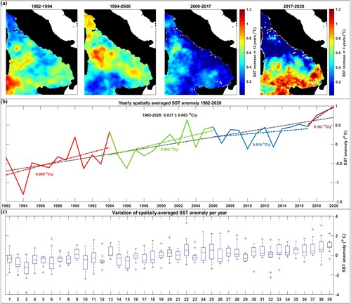
The basin-wide averaged temperature change during 2006–2017 was much lower than the long-term trend ((b)). Whereas, during the following years 2018, 2019 and 2020 an unprecedented strong surface warming was reported (the different phases are highlighted in ), leading to record values of basin-wide annual mean SSTs of 19.49°C, 19.61°C and 19.71°C, respectively. These record values surpassed even the annual mean SST of 2003 (19.38°C) which had held the title of the warmest year due to the extreme high summer SSTs that occurred during the well-known European heatwave in 2003 (Olita et al. Citation2007; Hobday et al. Citation2018).

Figure 3.6.2. (a) Hovmöller diagram (left) and intra-annual variations (right) of the spatially averaged SST per year, indicating significant changes in the seasonal cycle during 1982–2020. The monthly SST variations of the coldest year (1984), the three warmest years (2018, 2019, 2020) and the year of the European heatwave (2003) are highlighted for comparison with blue, shades of red and yellow, respectively. (b) SST phenology changes over the study area for the 39-year study period, showing the trend (at 95% confidence level) of the summer days (top), the summer onset (middle) and the trend of the summer end (bottom) based on the satellite-derived SST CMEMS product (Ref. No. 3.6.1 and 3.6.2).

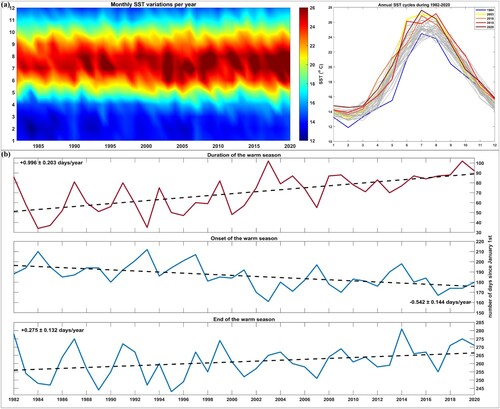
By analysing further the intra-annual characteristics of the observed surface warming, changes in the seasonal cycle became evident. While the basin-wide SST trends are generally stronger in summer (0.054 ± 0.003°C/year), a continuous tendency towards longer warm summer periods was found (see ). More specifically, the duration of the warm season has increased from 1982 to 2020 by more than a month (trends in (b)) as the season is starting ∼21 days earlier and ending ∼11 days later. These findings are alarming since even smaller changes in the seasonal SST cycle have been shown to influence the behaviour, growth, reproduction and survival of marine species (Edwards and Richardson Citation2004).

3.6.3.2. Extreme thermal events

The persistence of extreme thermal events in the Tyrrhenian Sea was additionally investigated. MHW events occurred on average at least twice a year, with maximum intensities of 2.44°C that lasted almost 14 days during 1982–2020. The strongest MHW occurred in 2003 and was characterised by an averaged maximum intensity of 5.64°C that lasted the entire summer. The corresponding highest daily SST ever measured occurred on 23^rd August 2003 with an exceptional basin-wide temperature of 28.7°C. Whereas their cold equivalent, MCS events, occurred on average once a year with maximum intensities of -2.17°C that persisted ∼11 days. The most intense individual MCS reached a basin-wide maximum intensity of -4.32°C in 1984. Respectively, the coldest basin-wide daily SST ever measured occurred on 29^th February of 1984 with record low SST of 11.8°C.

Moreover, as assessed in IPCC SROCC and AR6 for the global ocean (IPCC SROCC Citation2020; IPCC AR6 Citation2021), also the Tyrrhenian Sea showed significant changes in the magnitude and frequency of MHWs and MCSs over the past 4 decades. The results in reveal an increase in the frequency of MHWs with almost 5 additional events and exceeding anomalies of +0.59°C that last approximately 7 days longer. Moreover, the total number of annual MHW days has been increasing by almost 2 days each year, leading to a cumulative number of ∼74 more extreme warm days whilst more than half (54.25%) of the days with MHWs occurred in the last decade alone.

Figure 3.6.3. Time series of the annual basin-wide-averaged MHW (red) and MCS (blue) metrics together with their linear trends for the whole-time span (dotted line). These metrics were calculated following Hobday et al. (Citation2016) and Schlegel et al. (Citation2017) based on the daily satellite-derived SST CMEMS products (Ref. No. 3.6.1 and 3.6.2). Mean values are in units of annual event count (frequency), days (duration and total number of days with anomalous temperatures) and °C days for the integrated temperature anomaly during the event, equivalent to the sum of all daily intensity values (cumulative intensity). Trends (at 95% confidence level) are in the same units as the mean, per year.

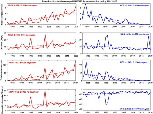
The frequency of MCSs, on the other hand, has been decreasing over the last 4 decades, leading to 4 fewer annual events which are characterised by less intense cold anomalies (+0.14°C) and approximately 4 days shorter durations. The total number of annual MCS days has been decreasing by more than 1 day each year, leading to a cumulative number of ∼51 fewer extreme cold days.

3.6.3.3. Extreme weather events

As in the ocean, extreme events in the atmosphere are also expected to have changed during the last decades with significant effects on human societies and ecosystems (IPCC SRCCL Citation2019; IPCC AR6 Citation2021). In the coastal area surrounding the Tyrrhenian Sea, 5445 extreme weather events have been reported in the last 39 years. The events consist of 9 main types () that were associated with numerous private and public damages, 541 registered injuries and 249 fatalities (based on the analysis of ESWD Ref. No. 3.6.4).

Figure 3.6.4. (a) Reported occurrences of extreme weather events (ESWD Ref. No. 3.6.4) in the coastal area (up to 0.5 degrees from the coastline) of the Tyrrhenian Sea. (b) Yearly values of the spatially averaged SST anomaly (CMEMS Ref. No. 3.6.1 and 3.6.2) indicating negative and positive anomalies with blue and red colours, respectively. (c) Yearly values of the spatially averaged convective available potential energy (CAPE) indicating the evolution of the mean atmospheric instability that can be used to assess the potential for the development of convection leading to severe weather events (ERA 5 Ref. No. 3.6.3). (d) Spatial distribution of the ESWD severe weather events associated with fatalities during the last 4 decades. Each circle represents the geographic location of an extreme event that caused fatalities, while the size indicates the severity (number of fatalities) and the colour the specific type of the event (ESWD Ref. No. 3.6.4). (e) Percentage of each extreme weather type that caused fatalities across the selected area during 1982–2020 based on reports from the European Severe Weather Database (ESWD Ref. No. 3.6.4).

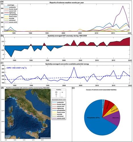
Using these reports as an indication of severe socio-economic impacts, it seems that the most catastrophic event type was heavy precipitation as it caused most (67%) of the registered fatalities ((d,e)) and frequently represented the main cause of severe damages. Reports of these extreme precipitation events and the resulting flash floods have shown an amplification of their frequency as well as of their severity, which can be attributed to the fact that more events were reported over time. In addition, 9 out of the top 10 deadliest events occurred in the last 12 years and were all caused by heavy precipitation.

3.6.4. Discussion and conclusions

Human communities in close connection with the ocean environment are particularly exposed to the occurring changes in the ocean and more than ever a long term, comprehensive and systematic monitoring, assessment and reporting of the ocean are required to ensure a sustainable science-based management for societal benefit (IPCC SROCC Citation2020).

Taking advantage of the longest freely available high-resolution satellite-derived SST dataset from the Copernicus Marine Environment Monitoring Service, we have shown that the surface temperatures in the Tyrrhenian Sea have been rising over the last 39 years with an average rate of 0.037°C/y which led to an accumulated warming of more than 1.44°C throughout the entire basin. The strong warming trend agrees with recent estimates concerning the Western Mediterranean Sea (0.036°C/y) during the period 1982–2018 (Pisano et al. Citation2020). The significant difference in the temporal SST variability of the two regions however (Krauzig et al. Citation2020), underlines the importance of local studies on sub-basin scales.

The long-term warming of the Tyrrhenian Sea was dominated by high increases of SST during the warm seasons, leading to significantly earlier and longer warm summer periods with an average extension of roughly 1 day every year. Given that the seasonal cycle accounts for the majority of the total SST variance, a lengthening of the warm summer season by more than a month is expected to have profound climatological and socio-ecological impacts (Kushnir et al. Citation2002; Keeling et al. Citation2010; Liu et al. Citation2020).

Additionally, as surface temperatures have been rising significantly during the last four decades, cold spells have become rarer and less severe, while marine heatwaves have become more severe, prolonged, and frequent. Even though changes in MHW/MCS frequency, intensity and duration are not simply a result of increasing mean SSTs (see also the discussion in section 1.7 by Dayan et al.), the projected SST warming under current greenhouse gas emission levels is expected to have a strong effect on MHW events (Collins et al. Citation2019; Oliver Citation2019).

Wakelin et al. (Citation2021) pointed out, that the impact of MHWs on marine ecosystems depends on the duration and amplitude of each event compared with the timescales of the ecological response and the susceptibility of the various components of the ecosystem. While some species might be able to gradually acclimatise to increasing temperatures in the presence of a long-term warming trend, species that are already living in the warmer end of their thermal preference spectrum are likely to exceeded critical temperature thresholds during MHW events (e.g. Marba and Duarte Citation2010). Furthermore, as warming trends favour a more stratified upper ocean (Li et al. Citation2020), impacts from accumulated heat stress and stratification are expected to surpass the coping capability of pelagic marine ecosystems and primary production (Cavole et al. Citation2016; Jacox et al. Citation2016; Smale et al. Citation2019).

At the same time, increasing numbers of extreme weather events with catastrophic impacts have been reported in the highly populated area surrounding the Tyrrhenian Sea. According to the latest IPCC reports (IPCC SROCC Citation2020; IPCC AR6 Citation2021), confidence has increased that some extremes will become even more frequent, widespread and intense during the twenty-first century at global scale. These events are among the most serious challenges to society in coping with a changing climate. In the Tyrrhenian Sea, the amplification of magnitude and frequency of reported extreme weather events led to significantly more damages, injuries and fatalities throughout the last 4 decades. Especially the increasing extreme precipitation events and the resulting flash floods have had catastrophic socio-economic impacts, costing at least 166 people their lives and leaving severe damages behind. Whilst flash floods are already considered the most frequent and among the costliest and deadliest natural disasters worldwide (Munich RE, NatCat Service; Swiss RE, 2015) the corresponding extreme precipitation events are expected to almost double per degree of further global warming (Myhre et al. Citation2019).

Several studies (Trenberth et al. Citation2015; Volosciuk et al. Citation2016; Dittus et al. Citation2018; Pastor et al. Citation2018) have shown that extreme precipitation events can be influenced by high SST through the recharge of moisture and heat and its contribution to increased conditional convective instability (i.e. Pastor et al. Citation2001; Lebeaupin et al. Citation2006; Alexander et al. Citation2009; Rebora et al. Citation2013; Messmer et al. Citation2017). Indeed, the overall trends in lower tropospheric moisture content (Specific humidity at 700 hPa: +6.16 ± 1.49×10–6 kg kg^-1/y) and convective available potential energy (CAPE: +1.54 ± 0.63 J kg^-1/y, (d)) could be a first indication that changes in thermodynamic instability and factors leading to convective initiation (following Taszarek et al. Citation2021) have become more favourable for heavy precipitation events. Further research into the potential role of SST changes in the occurrence of extreme precipitation events is therefore a promising avenue.

Our study provides insights into the prevalence of anomalous thermal events in the Tyrrhenian Sea and serves as a constructive first step to understand the risks of extreme weather events in the surrounding area. In the framework of climate change, these extremes and their nature need to be periodically monitored and analysed for future scenario projections that could help stakeholders in the establishment of mitigation and adaptation policies.

Section 3.7. Winter nutrient content as a basic proxy of ocean fertility

Authors: Donata Melaku Canu, Ginevra Rosati, Gianpiero Cossarini, Célia Laurent, Giorgio Bolzon, Cosimo Solidoro

Statement of main outcome: The capability of the oceans to sustain a productive and healthy ecosystem is one of the most important ecosystem services provided by the sea. Indeed, society is increasingly asking for indicators able to capture and deliver quantitative information on the spatial and year-to-year variability of these important ocean properties, also in order to support the implementation of sustainable approaches to marine spatial planning and to exploitation of biotic ocean resources.

Here we propose to compute ecosystem indicators related to trophic status and ocean fertility, derived from combinations of nutrient availability, primary productivity, chlorophyll, and fish landings. In particular, the abundance of nutrients in surface layers just after the winter mixing determines how fertile a region can be in the following spring and summer, since primary productivity relies on nutrient assimilation from the photic layer.

Several indices can be used to assess the trophic level of a water body and as a proxy of ocean fertility, from total chlorophyll concentration to multivariate indices such as TRIX and data on fish landings. Here we compute some of those indices and test whether or not they can be predicted in advance, as a function of the winter conditions described by CMEMS products.

Our results highlight that for most of the Mediterranean sub-basin the winter surface nutrient content, defined as the integral of nutrient concentration between the surface and the typical pycnocline depth of the sub-basin, can be used to predict months in advance the total amount of phytoplankton biomass to be developed in the following warm seasons, and in some cases provide some indications also on fish landings. This measure can therefore be considered as a first order index, and a predictor, of ocean fertility.

Products used in the analysis and documentation links:

Table

3.7.1. Introduction

In mid-latitude seas, often the plankton blooms start at the end of winter, as soon as light and temperature are suitable for photosynthesis and proceed as long as the inorganic nutrient dissolved in the upper part of the water column -originally homogenous because of winter mixing- is depleted. Indeed, the surface warming brought by the incoming spring creates a stratification which prevents – or strongly reduces- the vertical supply of nutrients from below the pycnocline up to the surface layers. At the same time, the stratification keeps the planktonic organisms in the upper part of the water column and if the critical depth (sensu Sverdrup, see Sverdrup Citation1953) is deeper than the pycnocline, the bloom develops as a subsurface spring bloom and lasts until the concentration of the most limiting nutrient in the upper part of the water column is close to zero. Meantime, part of the phytoplankton biomass is grazed by zooplankton and channelled along the food webs up to fishes (Mann and Lazier Citation2006; Libralato and Solidoro Citation2009). Therefore one might consider that, every year, all the nutrient in the upper part of the water column is later on assimilated by autotrophic organisms, and that the total amount of plankton biomass grown in a year is somehow constrained by the availability of nutrient in winter, computed as the sum of nutrients from the surface to the depth of the pycnocline (that will develop in the spring). Note that -as long as surface nutrient concentration during summer is close to zero- the surface concentration of winter can also be seen as the amount of nutrient brought to the surface during the cold season, and therefore as a winter nutrient fertilization index.

Here we tested this hypothesis by checking of the existence of a significant correlation between such a winter surface nutrient index, hereafter labelled ‘wsnc’ and the total amount of phytoplankton developed in spring and summer, by analysing the time series of those variables provided by 21 years long reanalysis of biogeochemical properties in the Mediterranean Sea, MEDSEA_MULTIYEAR_BGC_006_008, for each of 8 Mediterranean sub-basins (Cossarini et al. Citation2021).

We also test the possibilities of predicting yearly fish biomass estimates provided by FAO (www.fao.org/fishery/statistics/global-production/en), as a function of winter environmental variables, again for different Mediterranean sub-basins.

Other approaches can be used to explore the relationships between environmental properties and sea productivities (e.g. Rose et al. Citation2010; Béjaoui et al. Citation2018; Peck et al. Citation2018). Here we chose to focus our analysis only on the existence of the above-mentioned correlations, in order to test if, and to what extent, simple and easy to compute indices (such as wsnc) can capture and provide useful and important information on ocean productivity.

3.7.2. Methods

We based our analysis on the CMEMS reanalysis of biogeochemical and physical variables in the Mediterranean Sea (Data Ref #: 3.7.1, 3.7.2). Starting from the monthly mean profiles, we computed monthly values of integrated chlorophyll and integrated nutrients over the upper layers (from surface to a cut-off depth) from 1999 to 2019 (21 years providing 252 data points for each variable) and for each of the 8 Mediterranean sub-basins normally considered in CMEMS, i.e. Alboran Sea (ALB) the South Western Mediterranean (SWM), the North Western Mediterranean (NWM), the Tyrrhenian Sea (TYR), the Adriatic Sea (ADR), the Aegean Sea (AEG), the Ionian Sea (ION), the Levantine Sea (LEV). The cut-off depths for the integration of variables were evaluated by inspecting the time evolution of chlorophyll profiles and identifying the depth above which the time variability of chlorophyll concentration became very low, and much lower than above. In this way, we set the cut-off depth to 150 m in the Western Mediterranean Sea and to 200 m in the Eastern Mediterranean Sea, with the exception of the Adriatic Sea, where biogeochemical dynamics are mostly occurring in the top 100 m. The spatially integrated monthly values were then aggregated to derive seasonal values.

As an example, the winter surface nutrient index, wsnc, is defined as (3.7.1) $wsnc = \sum_{i = jan}^{march} \sum_{j = 1}^{z c} n u t_{i, j}$ (3.7.1) where zc is the cut-off depth introduced above, and nut_i,j is the concentration of the nutrient limiting phytoplankton growth at depth j.

A correlation matrix has then been computed among all couples of integrated variables, and simple and multiple linear regression models developed for synthetising annual biogeochemical variability.

The data set was then integrated with FAO fishery landings data from 1999 to 2018 (Data Ref #: 3.7.3) available for subbasins NWM, TYR, ION, LEV, ADR, and AEG, and used to investigate relationships between winter nutrient fertilization, plankton dynamics and fish landings, through the use of multiple linear regression models.

Finally, the climatology of wsnc is produced, in order to highlight standard reference behaviour and year-to-year variability.

3.7.3. Results

The correlation plots for the Mediterranean sub-basins show parameter distribution and correlation for each variable pair. depicts the plot for one of the sub-basins (ION) as an example. provides a summary of the results. The analysis shows that phytoplankton biomasses and chlorophyll concentrations were significantly correlated to PO4 and NOx concentrations in most cases (), except the ALB subbasin where no relation was found, likely because of the strong influence of the Gibraltar Strait. For the SWM and TYR the correlations coefficients for phytoplankton biomasses are about 0.4, but in the SWM the correlation is significant only for PO4 and not for NOx. In the NWM, AEG, ION and LEV coefficients are higher and significant. The correlations coefficients for chlorophyll tend to be lower than those for biomasses, except for the Adriatic Sea where chlorophyll seems to be better predicted. We note that while chlorophyll is frequently used as an indicator of productivity, chlorophyll is only a proxy of plankton biomass, which remains a much more direct and meaningful indicator of plankton productivity. Indeed, the Carbon to Chlorophyll ratio in plankton can vary quite a lot, as a function of nutrient limitation, light, and cell state (Geider et al. Citation1998; Lazzari et al. Citation2012).

Figure 3.7.1. Correlation plot for the biogeochemical dynamics in the Ionian Sea. ‘Summ’ is computed as the sum of June, July and August concentrations, while ‘Wint’ is the sum of January, February and March values. Chl is for chlorophyll (mg/m3), phy is for phytoplankton carbon biomasses (mgC/m3), PO4 is for phosphate (mgP/m3), NOx is for nitrate and nitrite (mgN/m3), TRIX is a trophic index calculated as $TRIX = \frac{1}{1.2} (\log NO x + \log PO 4 + \log Chl + 1.5)$ (Vollenweider et al. Citation1988), Temp is water temperature and Sal is salinity. Significance levels: ‘***’ = 0, ‘**’< 0.001, ‘*’< 0.01, ‘▪’< 0.05, ‘·’ n.s.

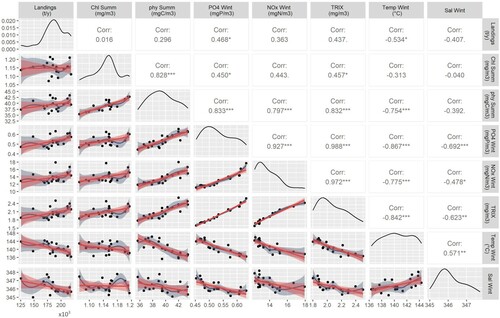
Table 3.7.1. Synthesis of the correlation coefficients between winter nutrient concentrations and summer phytoplankton biomasses and chlorophyll concentrations, and fish landings for Mediterranean Sea sub-basins. Grey numbers indicate non-significant correlations.

As for biomass, factors others than nutrients can contribute to defining plankton dynamics, including irradiance and water transparency, vertical diffusion, the sinking rate of planktonic cells, and grazing pressure (Jamar et al. Citation1977; Mann and Lazier Citation2006), so that it is not surprising to see that different regions present different correlations between nutrients and plankton biomass. In particular, the correlation can decrease whenever horizontal processes become as significant as vertical processes, as well as in spatially highly heterogenous regions, where a single spatially averaged value cannot provide a sufficiently detailed picture of the system. The relationships between nutrients and fish abundance is even more complex, since different species of fish feed on different preys and have different trophic levels and therefore some species are more loosely related to plankton biomass than others. Furthermore, in this study we used the FAO landings data, that are fishery dependent observations bound to overestimate commercially valuable species relative to others.

The analysis of correlations including fish landing data, where available, shows weak or no linear correlation, in most sub-basins ().

Taking into account more than one predictor, the results of the multiple regressions indicate that in the eastern part of the Mediterranean, EMED (sum of LEV, AEG, ADR, ION subbasins), 65% of the variation of summer chlorophyll and 69% of the variation of summer phytoplankton biomasses can be explained taking into account winter nutrients, salinity and/or temperature, while in the western Mediterranean, WMED, the variability explained amounts to 85% for chlorophyll and 90% for biomasses.

The resulting regression equations are given in , together with the best models for fish landing data. Multiple regression analyses have the capability to significantly predict fish landings when past dynamics are included. In particular, we found that a model (model M1, Equation 3.7.2) taking into account the landing of the previous year and the summer temperature of the current year is a good predictor for NWM, TYR, AEG, ION and LEV (). However, in NWM, TYR, and LEV, the relation with temperature is not significant, and thus the equation is reduced to a simple linear model ().

Table 3.7.2. Significant regressions for Mediterranean Sea sub-basins from the multiple regression analysis carried out with Chlorophyll, Phytoplankton biomass, landings data and CMEMS biogeochemical variables.

Display Table

For the ADR sub-basin, a more complex model (M2, Equation 3.7.3) has to be used, taking into account winter temperature and the zooplankton biomass observed two years in advance, but no landings of previous years. This regression model is also a better predictor than the previous one in the LEV subbasin, but in this case the catches of the previous year remain relevant and winter temperature is not important. If those models are combined, temperature becomes less significant. (3.7.2) $M 1 F i s h L_{y} = f (F i s h L_{y - 1}, T e m p_{s u m})$ (3.7.2) (3.7.3) $M 2 F i s h L_{y} = f (F i s h L_{y - 1}, Z o o_{y - 2}, T e m p_{w i n})$ (3.7.3)

Other significant correlations used as predictors the winter surface nutrient content observed two years in advance, possibly suggesting that fish dynamics depend on biogeochemical properties over longer time intervals, as well as the TRIX index (Vollenweider et al. Citation1998) of the previous summer, again stressing the relevance of taking into consideration the importance of the trophic level over time scales longer than a year, and possibly related to the lifespan of fish. In all of these models, however, the contribution of nutrient (or TRIX) predictors is lower than the contribution of previous year catches. These results offer further support to the conclusion that fish population dynamics is affected by environmental conditions through the superposition of different processes, including nutrient availability and temperature, but the relationships among these variables are complex and possibly mediated by intermediate variables, such as zooplankton biomass. (3.7.4) $M 3 F i s h L_{y} = f (F i s h L_{y - 1}, N O x_{w i n - 2}, T e m p_{s u m})$ (3.7.4) (3.7.5) $M 4 F i s h L_{y} = f (F i s h L_{y - 1}, T r i x_{y - 1}, T e m p_{w i n})$ (3.7.5)

Finally, provides the evolution of the anomaly of such indices for each of the basins over 1999–2019 highlighting the prevalence of positive anomaly in the first years of this period and negative anomalies in the last decade.

Figure 3.7.2. Annual variability of winter surface contents in the different Mediterranean sub-basins, relative to each sub-basin climatological value.

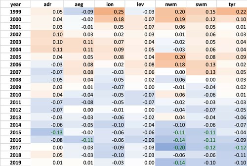
3.7.4. Conclusion

For most of the Mediterranean sub-basins, the winter surface nutrient content index, defined as the integral of nutrient concentration between the surface and the typical euphotic depth of a sub-basin and over winter months (see Equation (3.7.1)), is significantly correlated to the plankton productivity, captured by the total summer chlorophyll concentration or, even better, by the total phytoplankton biomass. In some cases, fish biomass landing can also be predicted. Therefore, this index can be seen as a basic predictor able to provide indications on the productivity expected in the upcoming spring and summer seasons. The capability to predict chlorophyll and phytoplankton biomass increases when using multiple regression models (i.e. more than one predictor) using both nitrogen and phosphorus but also temperature and salinity values. The use of multiple regression models, however, does not increase the capability of predicting fish landings, unless fish past abundance is considered, in some cases also in conjunction with the winter nutrient concentration of 2 years before. These facts, while confirming that the dynamic underpinning the relationship between fishes and nutrient mixing is more complex than the one between nutrients mixing and plankton, also confirm that such a relationship exists, and that indices based on winter properties can also be informative for sea productivity at the fish level. However, more complex relationships should be considered, and possibly spanning longer time windows. The use of the simpler winter surface nutrient content index therefore appears appropriate as a first order index, and predictor, of ocean fertility.

Supplemental material

Supplemental Material

Supplemental Material

References

Agusti S, Martinez-Ayala J, Regaudie-de-Gioux A, Duarte CM. 2017. Oligotrophication and metabolic slowing-down of a NW Mediterranean coastal ecosystem. Front Mar Sci. 4:432. doi:10.3389/fmars.2017.00432.
Web of Science ®Google Scholar
Alamanos A, Linnane S. 2021. Estimating SDG indicators in data-scarce areas: the transition to the use of new technologies and multidisciplinary studies. Earth. 2:635–652. doi:10.3390/earth2030037.
Google Scholar
Anderson DM, Glibert PM, Burkholder JM. 2002. Harmful algal blooms and eutrophication: nutrient sources, composition, and consequences. Estuaries. 25:704–726. doi:10.1007/BF02804901.
Google Scholar
Andersen JH, Kallenbach E, Murray C, Ledang AB. 2016. Eutrophication in the Danish parts of the North Sea, Skagerrak and Kattegat 2006–2014. A literature-based status assessment. NIVA Denmark Report. https://brage.bibsys.no/xmlui/handle/11250/2406499.
Google Scholar
Anderson K, Ryan B, Sonntag W, Kavvada A, Friedl L. 2017. Earth observation in service of the 2030 agenda for sustainable development. Geo Spatial Inf Sci. 20:77–96. doi:10.1080/10095020.2017.1333230.
Google Scholar
Attila J, Kauppila P, Kallio KY, Alasalmi H, Keto V, Bruun E, Koponen S. 2018. Applicability of earth observation chlorophyll-a data in assessment of water status via MERIS – with implications for the use of OLCI sensors. Remote Sens Environ. 212:273–287. doi:10.1016/j.rse.2018.02.043.
Web of Science ®Google Scholar
Balmer MB, Downing JA. 2011. Carbon dioxide concentrations in eutrophic lakes: undersaturation implies atmospheric uptake. Inland Waters. 1(2):125–132. doi:10.5268/IW-1.2.366.
Web of Science ®Google Scholar
Baretta-Bekker H, Sell A, Marco-Rius F, Wischnewski J, Walsham P, Malin Mohlin L, Wesslander K, Ruiter H, Gohin F, Enserink L. 2015. The chlorophyll case study in the JMP NS/CS project. Document produced as part of the EU project: ‘Towards joint Monitoring for the North Sea and Celtic Sea’ (Ref: ENV/PP 2012/SEA).
Google Scholar
Brando VE, Sammartino M, Colella S, Bracaglia M, Di Cicco A, D’Alimonte D, Kajiyama T, Kaitala S, Attila J. 2021. Phytoplankton bloom dynamics in the Baltic Sea using a consistently reprocessed time series of multi-sensor reflectance and novel chlorophyll-a retrievals. Remote Sens. 13:3071.
Google Scholar
Breitburg D, Levin LA, Oschlies A, Grégoire M, Chavez FP, Conley DJ, Garçon V, Gilbert D, Gutiérrez D, Isensee K, Jacinto GS. 2018. Declining oxygen in the global ocean and coastal waters. Science. 359(6371):eaam7240.
PubMed Web of Science ®Google Scholar
Brush MJ, Giani M, Totti C, Testa JM, Faganeli J, Ogrinc N, Kemp MW, Fondi-Umani S. 2020. Eutrophication, harmful algae, oxygen depletion, and acidification. Coastal Ecosystems in Transition: A Comparative Analysis of the Northern Adriatic and Chesapeake Bay, 75–104.
Google Scholar
Cai W, Hu X, Huang W. 2011. Acidification of subsurface coastal waters enhanced by eutrophication. Nature Geosci. 4:766–770. doi:10.1038/ngeo1297.
Web of Science ®Google Scholar
Carvalho L, Mackay EB, Cardoso AC, Baattrup-Pedersen A, Birk S, Blackstock KL, Borics G, Borja A, Feld CK, Ferreira MT, et al. 2019. Protecting and restoring Europe’s waters: an analysis of the future development needs of the water framework directive. Sci Total Environ. 658:1228–1238. doi:10.1016/j.scitotenv.2018.12.255.
PubMed Web of Science ®Google Scholar
CMEMS OMI catalogue. 2020. ATLANTIC_OMI_HEALTH_OceanColour_anomalies https://resources.marine.copernicus.eu/?option=com_csw&view=details&product_id=ATLANTIC_OMI_HEALTH_OceanColour_anomalies.
Google Scholar
Colella S, Falcini F, Rinaldi E, Sammartino M, Santoleri R. 2016. Mediterranean ocean colour chlorophyll trends. PLoS One. 11(6):e0155756.
PubMed Web of Science ®Google Scholar
Coppini G, Lyubartsev V, Pinardi N, Colella S, Santoleri R, Christiansen T. 2012. Chl-a trends in European seas estimated using ocean-colour products. Ocean Science Discussions. 9:1481–1518. doi:10.5194/osd-9-1481-2012.
Google Scholar
Cristina S, Icely J, Goela PC, DelValls TA, Newton A. 2015. Using remote sensing as a support to the implementation of the European Marine Strategy Framework Directive in SW Portugal. Cont Shelf Res. 108:169–177.
Web of Science ®Google Scholar
Duarte CM, Regaudie-de-Gioux A, Arrieta JM, Delgado-Huertas A, Agusti S. 2013. The oligotrophic ocean is heterotrophic. Ann Rev Mar Sci. 5:551–569.
PubMed Web of Science ®Google Scholar
Estoque RC. 2020. A review of the sustainability concept and the state of SDG monitoring using remote sensing. Remote Sens. 12:1770. doi:10.3390/rs12111770.
Google Scholar
Eurostat. 2021. Sustainable development in the European Union. Monitoring report on progress towards the SDGs in an EU context. ISBN 978-92-76-30698-6, Cat. No: KS-03-21-096-EN-N. doi:10.2785/195273.
Google Scholar
European Environment Agency. 2019a. Marine Messages II’ Navigating the course towards clean, healthy and productive seas through implementation of an ecosystem-based approach. EEA Report No 17/2019 ISSN 1977-8449.
Google Scholar
European Environment Agency. 2019b. Nutrient enrichment and eutrophication in Europe's seas. Moving towards a healthy marine environment EEA Report No 14/2019 ISSN1977-8449.
Google Scholar
Friedland R, Macias DM, Cossarini G, Daewel U, Estournel C, Garcia-Gorriz E, Grizzetti B, Grégoire M, Gustafson B, Kalaroni S, et al. 2021. Effects of nutrient management scenarios on marine eutrophication indicators: a Pan-European, multi-model assessment in support of the Marine Strategy Framework Directive. Front Mar Sci. 8. doi:10.3389/fmars.2021.596126.
PubMed Web of Science ®Google Scholar
Galloway JN, Townsend AR, Erisman JW, Bekunda M, Cai Z, Freney JR, Martinelli LA, Seitzinger SP, Sutton MA. 2008. Transformation of the nitrogen cycle: recent trends, questions, and potential solutions. Science. 320(5878):889–892. doi:10.1126/science.1136674.
PubMed Web of Science ®Google Scholar
GEO Blue Planet. 2021. Global eutrophication monitoring in support of SDG 14. [accessed 2021 Jul 30]. https://geoblueplanet.org/blue-planet-activities/eutrophication/.
Google Scholar
Gohin F, Bryère P, Lefebvre A, Sauriau P-G, Savoye N, Vantrepotte V, Bozec Y, Cariou T, Conan P, Coudray S, et al. 2020. Satellite and in situ monitoring of chl-a, turbidity, and total suspended matter in coastal waters: experience of the year 2017 along the French coasts. J Mar Sci Eng. 8(9):665. doi:10.3390/jmse8090665.
Web of Science ®Google Scholar
Gohin F, Saulquin B, Oger-Jeanneret H, Lozac’h L, Lampert L, Lefebvre A, Riou P, Bruchon F. 2008. Towards a better assessment of the ecological status of coastal waters using satellite-derived chlorophyll-a concentrations. Remote Sens Environ. 112:3329–3340.
Web of Science ®Google Scholar
Gohin F, Van der Zande D, Tilstone G, Eleveld MA, Lefebvre A, Andrieux-Loyer F, Blauw AN, Bryère P, Devreker D, Garnesson P, et al. 2019. Twenty years of satellite and in situ observations of surface chlorophyll-a from the northern Bay of Biscay to the eastern English Channel. Is the water quality improving? Remote Sens Environ. 233:111343. doi:10.1016/j.rse.2019.111343.
Web of Science ®Google Scholar
Groetsch PMM, Simis SGH, Eleveld MA, Peters SWM. 2016. Spring blooms in the Baltic Sea have weakened but lengthened from 2000 to 2014. Biogeosciences. 13(17):4959–4973. doi:10.5194/bg-13-4959-2016.
Web of Science ®Google Scholar
Harvey ET, Kratzer S, Philipson P. 2015. Satellite-based water quality monitoring for improved spatial and temporal retrieval of chlorophyll-a in coastal waters. Remote Sens Environ. 158:417–430. doi:10.1016/j.rse.2014.11.017.
Web of Science ®Google Scholar
Howarth RW, Anderson D, Cloern J, Elfring C, Hopkinson C, Lapointe B, Malone T, Marcus N, McGlathery K, Sharpley A, Walker D. 2000. Nutrient pollution of coastal rivers, bays and seas. Issues Ecol. 7:1–16.
Google Scholar
Howarth RW, Marino R. 2006. Nitrogen as the limiting nutrient for eutrophication in coastal marine ecosystems: evolving views over three decades. Limnol Oceanogr. 51(1, part 2). doi:10.4319/lo.2006.51.1_part_2.0364.
PubMed Web of Science ®Google Scholar
Hutchinson GE. 1969. Eutrophication, past and present. In: Eutrophication: Causes, Consequences, Correctives, p. 17-26. National Academy of Sciences, Washington, DC.
Google Scholar
Jickells TD. 1998. Nutrient biogeochemistry of the coastal zone. Science. 281:217–222. doi:10.1126/science.281.5374.217.
PubMed Web of Science ®Google Scholar
Karydis M, Kitsiou D. 2019. Marine eutrophication: a global perspective. Boca Raton, FL: CRC Press. 193 pp.
Google Scholar
Malone TC, Newton A. 2020. The globalization of cultural eutrophication in the coastal ocean: causes and consequences. Front Mar Sci. 7:670. doi:10.3389/fmars.2020.00670.
Web of Science ®Google Scholar
Masó J, Serral I, Domingo-Marimon C, Zabala A. 2020. Earth observations for sustainable development goals monitoring based on essential variables and driver-pressure-state-impact-response indicators. Int J Digital Earth. 13(2):217–235. doi:10.1080/17538947.2019.1576787.
Web of Science ®Google Scholar
Maúre EDR, Terauchi G, Ishizaka J, Clinton N, DeWitt M. 2021. Globally consistent assessment of coastal eutrophication. Nat Commun. 12:6142. doi:10.1038/s41467-021-26391-9.
PubMed Web of Science ®Google Scholar
Nixon SW. 1995. Coastal marine eutrophication: a definition, social causes, and future concerns. Ophelia, 41:199-219.
Web of Science ®Google Scholar
OSPAR ICG-EUT. Axe P, Clausen U, Leujak W, Malcolm S, Ruiter H, Prins T, Harvey ET. (2017). Eutrophication status of the OSPAR Maritime Area. Third integrated report on the eutrophication status of the OSPAR Maritime Area.
Google Scholar
Pardo S, Sathyendranath S, Platt T. 2021. 2.4 eutrophic and oligotrophic indicators for the North Atlantic Ocean. J Oper Oceanogr. 14(S1):1–185. doi:10.1080/1755876X.2021.1946240.
Google Scholar
Park Y, Ruddick K, Lacroix G. 2010. Detection of algal blooms in European waters based on satellite chlorophyll data from MERIS and MODIS. Int J Remote Sens. 31:6567–6583.
Web of Science ®Google Scholar
Sathyendranath S, Brewin RJW, Brockmann C, Brotas V, Calton B, Chuprin A, Cipollini P, Couto AB, Dingle J, Doerffer R, et al. 2019. An ocean-colour time series for use in climate studies: the experience of the ocean-colour climate change initiative (OC-CCI). Sensors. 19:4285. doi:10.3390/s19194285.
Web of Science ®Google Scholar
Sathyendranath S, Platt T, Kovač Ž, Dingle J, Jackson T, Brewin RJW, Franks P, Marañón E, Kulk G, Bouman HA. 2020. Reconciling models of primary production and photoacclimation. Appl Opt. 59:C100–C114. doi:10.1364/AO.386252.
PubMed Web of Science ®Google Scholar
Schindler DW. 2006. Recent advances in the understanding and management of eutrophication. Limnol Oceanogr. 51:356–363.
Web of Science ®Google Scholar
Smith VH. 2003. Eutrophication of freshwater and coastal marine ecosystems a global problem. Environ Sci Pollut Res. 10:126–139. doi:10.1065/espr2002.12.142.
PubMed Web of Science ®Google Scholar
Seitzinger S, Mayorga E. 2016. Nutrient inputs from river systems to coastal waters. In IOC-UNESCO and UNEP, editors. Large marine ecosystems: status and trends. United Nations Environment Programme. Chapter 7.3. p. 179–195. http://www.geftwap.org/publications/lmes-technical-report.
Google Scholar
UNEP. 2021. Understanding the State of the Ocean: a global manual on measuring SDG 14.1.1, SDG 14.2.1 and SDG 14.5.1. Nairobi: UNEP.
Google Scholar
Van der Zande D, Lavigne H, Blauw A, Prins T, Desmit X, Eleveld M, Gohin F, Pardo S, Tilstone G, Cardoso Dos Santos J. 2019. Enhance coherence in eutrophication assessments based on chlorophyll, using satellite data as part of the EU project ‘Joint monitoring programme of the eutrophication of the North Sea with satellite data’ (Ref: DG ENV/MSFD Second Cycle/2016). Activity 2 Report.
Google Scholar
Van Meerssche E, Pinckney JL. 2019. Nutrient loading impacts on estuarine phytoplankton size and community composition: community-based indicators of eutrophication. Estuaries Coasts. 42:504–512. doi:10.1007/s12237-018-0470-z.
Web of Science ®Google Scholar
VLIZ. 2019. Maritime boundaries geodatabase: maritime boundaries and exclusive economic zones (200NM), version 11. Flanders Marine Institute. doi:10.14284/386.
Google Scholar
Wallace RB, Baumann H, Grear JS, Aller RB, Gobler CJ. 2014. Coastal ocean acidification: the other eutrophication problem. Estuarine Coastal Shelf Sci. 148:1–13. doi:10.1016/j.ecss.2014.05.027.
Web of Science ®Google Scholar
Williams PJLB, Quay PD, Westberry TK, Behrenfeld MJ. 2013. The oligotrophic ocean is autotrophic. Ann Rev Mar Sci. 5:535–549.
PubMed Web of Science ®Google Scholar
Zingone A, Phlips EJ, Harrison PJ. 2010. Multiscale variability of twenty-two coastal phytoplankton time series: a global scale comparison. Estuaries Coasts. 33:224–229. doi:10.1007/s12237-009-9261-x.
Web of Science ®Google Scholar
Andersen JH, Carstensen J, Conley DJ, Dromph C, Fleming-Lehtinen V, Gustafsson BG, Josefson AB, Norkko A, Villnäs A, Murray C. 2017. Long-term temporal and spatial trends in eutrophication status of the Baltic Sea. Biol Rev. 92:135–149. doi:10.1111/brv.12221.
PubMed Web of Science ®Google Scholar
Conley DJ, Björck S, Bonsdorff E, Carstensen J, Destouni G, Gustafsson BG, Hietanen S, Kortekaas M, Kuosa H, Meier HEM, et al. 2009. Hypoxia-related processes in the Baltic Sea. Environ Sci Technol. 43(10):3412–3420. doi:10.1021/es802762a.
PubMed Web of Science ®Google Scholar
Dalsgaard T, De Brabandere L, Hall POJ. 2013. Denitrification in the water column of the central Baltic Sea. Geochim Cosmochim Acta. 106:247–260. doi:10.1016/j.gca.2012.12.038.
Web of Science ®Google Scholar
Danielsson Å, Papush L, Rahm L. 2008. Alterations in nutrient limitations – scenarios of a changing Baltic Sea. J Mar Sys. 73(3–4):263–283. doi:10.1016/j.jmarsys.2007.10.015.
Web of Science ®Google Scholar
Deutsch B, Forster S, Wilhelm M, Dippner JW, Voss M. 2010. Denitrification in sediments as a major nitrogen sink in the Baltic Sea: an extrapolation using sediment characteristics. Biogeosciences. 7(10):3259–3271. doi:10.5194/bg-7-3259-2010.
Web of Science ®Google Scholar
Egge JK, Aksnes DL. 1992. Silicate as regulating nutrient in phytoplankton competition. Mar Ecol Prog Ser. 83(2–3):281–289. doi:10.3354/meps083281.
Web of Science ®Google Scholar
Farcy P, Durand D, Charria G, Painting SJ, Tamminen T, Collingridge K, Grémare AJ, Delauney L, Puillat I. 2019. Toward a European coastal observing network to provide better answers to science and to societal challenges; the JERICO research infrastructure. Front Mar Sci. 6:529. doi:10.3389/fmars.2019.00529.
Web of Science ®Google Scholar
Fleming-Lehtinen V, Andersen JH, Carstensen J, Łysiak-Pastuszak E, Murray C, Pyhälä M, Laamanen M. 2015. Recent developments in assessment methodology reveal that the Baltic Sea eutrophication problem is expanding. Ecol Indic. 48:380–388. doi:10.1016/j.ecolind.2014.08.022.
Web of Science ®Google Scholar
Fleming-Lehtinen V, Laamanen M, Kuosa H, Haahti H, Olsonen R. 2008. Long-term development of inorganic nutrients and chlorophyll α in the open Northern Baltic Sea long-term development of inorganic nutrients and chlorophyll a in the open Northern Baltic Sea. Ambio. 37:86–92. doi:10.1579/0044-7447.
PubMed Web of Science ®Google Scholar
Fleming V, Kaitala S. 2006. Phytoplankton spring bloom intensity index for the Baltic Sea estimated for the years 1992 to 2004. Hydrobiologia. 554:57–65. doi:10.1007/s10750-005-1006-7.
Web of Science ®Google Scholar
García-García LM, Sivyer D, Devlin M, Painting S, Collingridge K, van der Molen J. 2019. Optimizing monitoring programs: a case study based on the OSPAR eutrophication assessment for UK waters. Front Mar Sci. 5:503. doi:10.3389/fmars.2018.00503.
Web of Science ®Google Scholar
Graneli E, Wallstrom K, Larsson U, Graneli W, Elmgren R. 1990. Nutrient limitation of primary production in the Baltic Sea area. Ambio. 19(3):142–151. doi:10.2307/4313680.
Web of Science ®Google Scholar
Grasshoff K, Kremling K, Ehrhardt M. 1999. Methods of seawater analysis. 3rd ed. New York: Wiley-VCH.
Google Scholar
Gustafsson BG, Schenk F, Blenckner T, Eilola K, Meier HEM, Müller-Karulis B, Neumann T, Ruoho-Airola T, Savchuk OP, Zorita E. 2012. Reconstructing the development of Baltic Sea eutrophication 1850–2006. Ambio. 41(6):534–548. doi:10.1007/s13280-012-0318-x.
PubMed Web of Science ®Google Scholar
Gustafsson E, Savchuk OP, Gustafsson BG, Müller-Karulis B. 2017. Key processes in the coupled carbon, nitrogen, and phosphorus cycling of the Baltic Sea. Biogeochemistry. 134(3):301–317. doi:10.1007/s10533-017-0361-6.
Web of Science ®Google Scholar
HELCOM. 2017. Manual for marine monitoring in the COMBINE program of HELCOM. Last updated: July 2017. https://helcom.fi/action-areas/monitoring-and-assessment/monitoring-guidelines/combine-manual/.
Google Scholar
HELCOM. 2018a. State of the Baltic Sea – Second HELCOM holistic assessment, 2011–2016. Baltic Sea Environment Proceedings 155. http://stateofthebalticsea.helcom.fi/pressures-and-their-status/hazardous-substances/.
Google Scholar
HELCOM. 2018b. HELCOM thematic assessment of eutrophication 2011–2016. Baltic Sea Environment Proceedings 156. http://www.helcom.fi/baltic-sea-trends/holistic-assessments/state-of-the-baltic-sea-2018/reports-and-materials/.
Google Scholar
Humborg C, Smedberg E, Medina MR, Mörth CM. 2008. Changes in dissolved silicate loads to the Baltic Sea – the effects of lakes and reservoirs. J Mar Sys. 73(3–4):223–235. doi:10.1016/j.jmarsys.2007.10.014.
Web of Science ®Google Scholar
Kahru M, Elmgren R. 2014. Multidecadal time series of satellite-detected accumulations of cyanobacteria in the Baltic Sea. Biogeosciences. 11:3619–3633. doi:10.5194/bg-11-3619-2014.
Web of Science ®Google Scholar
Klais R, Tamminen T, Kremp A, Spilling K, Olli K. 2011. Decadal-scale changes of dinoflagellates and diatoms in the anomalous Baltic Sea spring bloom. PLoS One. 6(6):e21567. doi:10.1371/journal.pone.0021567.
PubMed Web of Science ®Google Scholar
Kõuts M, Maljutenko I, Elken J, Liu Y, Hansson M, Viktorsson L, Raudsepp U. 2021. Recent regime of persistent hypoxia in the Baltic Sea. Environ Res Commun. 3:075004. doi:10.1088/2515-7620/ac0cc4.
Google Scholar
Kõuts M, Maljutenko I, Liu Y, Raudsepp U. 2021. 2.5 Nitrate, ammonium and phosphate pools in the Baltic Sea. In: Copernicus Marine Service Ocean State Report, Issue 5. J Oper Oceanogr. 14(suppl. 1). doi:10.1080/1755876X.2021.1946240.
Google Scholar
Lehtoranta J, Savchuk OP, Elken J, Dahlbo K, Kuosa H, Raateoja M, Kauppila P, Räike A, Pitkänen H. 2017. Atmospheric forcing controlling inter-annual nutrient dynamics in the open Gulf of Finland. J Mar Sys. 171:4–20. doi:10.1016/j.jmarsys.2017.02.001.
Web of Science ®Google Scholar
Murray CJ, Müller-Karulis B, Carstensen J, Conley DJ, Gustafsson BG, Andersen JH. 2019. Past, present and future eutrophication status of the Baltic Sea. Front Mar Sci. 6:2. doi:10.3389/fmars.2019.00002.
Web of Science ®Google Scholar
Ohlendieck U, Stuhr A, Siegmund H. 2000. Nitrogen fixation by diazotrophic cyanobacteria in the Baltic Sea and transfer of the newly fixed nitrogen to picoplankton organisms. J Mar Sys. 25(3–4):213–219. doi:10.1016/S0924-7963(00)00016-6.
Web of Science ®Google Scholar
Olofsson M, Klawonn I, Karlson B. 2021. Nitrogen fixation estimates for the Baltic Sea indicate high rates for the previously overlooked Bothnian Sea. Ambio. 50(1):203–214. doi:10.1007/s13280-020-01331-x.
PubMed Web of Science ®Google Scholar
Pilkaityte R, Razinkovas A. 2007. Seasonal changes in phytoplankton composition and nutrient limitation in a shallow Baltic lagoon. Boreal Environ Res. 12(5):551–559.
Web of Science ®Google Scholar
Raateoja M, Kuosa H, Hällfors S. 2011. Fate of excess phosphorus in the Baltic Sea: a real driving force for cyanobacterial blooms? J Sea Res. 65(2):315–321. doi:10.1016/j.seares.2011.01.004.
Web of Science ®Google Scholar
Raateoja M, Hällfors H, Kaitala S. 2018. Vernal phytoplankton bloom in the Baltic Sea: intensity and relation to nutrient regime. J Sea Res. 138:24–33. doi:10.1016/j.seares.2018.05.003.
Web of Science ®Google Scholar
Räike A, Taskinen A, Knuuttila S. 2020. Nutrient export from Finnish rivers into the Baltic Sea has not decreased despite water protection measures. Ambio. 49(2):460–474. doi:10.1007/s13280-019-01217-7.
PubMed Web of Science ®Google Scholar
Rantajärvi E. 2003. Alg@line in 2003: 10 years of innovative plankton monitoring and research and operational information service in the Baltic Sea. Meri Report Series of the Finnish Institute of Marine Research. 48.
Google Scholar
Rantajärvi E, Pitkänen H, Korpinen S, Nurmi M, Ekebom J, Liljaniemi P, Cederberg T, Suomela J, Paavilainen P, Lahtinen T. 2020. Manual for marine monitoring in Finland 2020–2026. Suomen ympäristökeskuksen raportteja. 47 (in Finnish), 219 pages.
Google Scholar
Rönnberg C, Bonsdorff E. 2004. Baltic Sea eutrophication: area-specific ecological consequences. Hydrobiologia. 514(2002):227–241. doi:10.1023/B:HYDR.0000019238.84989.7f.
Google Scholar
Ruokanen L, Kaitala S, Fleming V, Maunula P. 2003. Alg@line-joint operational unattended phytoplankton monitoring in the Baltic Sea. In: Dahlin H, Flemming NC, Nittis K, Petersson SE, editors. Elsevier oceanography series. Vol. 69. Elsevier; p. 519–522. doi:10.1016/S0422-9894(03)80083-1.
Google Scholar
Savchuk OP. 2018. Large-scale nutrient dynamics in the Baltic Sea, 1970–2016. Front Mar Sci. 5:1–20. doi:10.3389/fmars.2018.00095.
PubMed Web of Science ®Google Scholar
Snoeijs-Leijonmalm P, Schubert H, Radziejewska T. 2017. Biological oceanography of the Baltic Sea. Springer Science & Business Media, Dordrecht.
Google Scholar
Spilling K, Olli K, Lehtoranta J, Kremp A, Tedesco L, Tamelander T, Klais R, Peltonen H, Tamminen T. 2018. Shifting diatom – dinoflagellate dominance during spring bloom in the Baltic Sea and its potential effects on biogeochemical cycling. Front Mar Sci. 5:327. doi:10.3389/fmars.2018.00327.
Web of Science ®Google Scholar
Spilling K, Tamminen T, Andersen T, Kremp A. 2010. Nutrient kinetics modeled from time series of substrate depletion and growth: dissolved silicate uptake of Baltic Sea spring diatoms. Mar Biol. 157(2):427–436. doi:10.1007/s00227-009-1329-4.
Web of Science ®Google Scholar
Stal LJ, Albertano P, Bergman B, Von Bröckel K, Gallon JR, Hayes PK, Sivonen K, Walsby AE. 2003. BASIC: Baltic Sea cyanobacteria. An investigation of the structure and dynamics of water blooms of cyanobacteria in the Baltic Sea – responses to a changing environment. Cont Shelf Res. 23(17–19):1695–1714. doi:10.1016/j.csr.2003.06.001.
Web of Science ®Google Scholar
Tallberg P, Heiskanen AS, Niemistö J, Hall POJ, Lehtoranta J. 2017. Are benthic fluxes important for the availability of Si in the Gulf of Finland? J Mar Sys. 171:89–100. doi:10.1016/j.jmarsys.2017.01.010.
Web of Science ®Google Scholar
Tamminen T, Andersen T. 2007. Seasonal phytoplankton nutrient limitation patterns as revealed by bioassays over Baltic Sea gradients of salinity and eutrophication. Mar Ecol Prog Ser. 340(1971):121–138. doi:10.3354/meps340121.
Google Scholar
Wasmund N, Kownacka J, Göbel J, Jaanus A, Johansen M, Jurgensone I, Lehtinen S, Powilleit M. 2017. The diatom/dinoflagellate index as an indicator of ecosystem changes in the Baltic Sea 1. Principle and handling instruction. Front Mar Sci. 4:1–13. doi:10.3389/FMARS.2017.00022.
Web of Science ®Google Scholar
Wasmund N, Nausch G, Feistel R. 2013. Silicate consumption: an indicator for long-term trends in spring diatom development in the Baltic Sea. J Plankton Res. 35(2):393–406. doi:10.1093/plankt/fbs101.
Web of Science ®Google Scholar
Zdun A, Stoń-Egiert J, Ficek D, Ostrowska M. 2021. Seasonal and spatial changes of primary production in the Baltic Sea (Europe) based on in situ measurements in the period of 1993–2018. Front Mar Sci. 7. doi:10.3389/fmars.2020.604532.
Web of Science ®Google Scholar
Andréfouët S, Van Wynsberge S, Kabbadj L, Wabnitz CC, Menkès C, Tamata T, Pahuatini M, Tetairekie I, Teaka I, Scha TA, et al. 2018. Adaptive management for the sustainable exploitation of lagoon resources in remote islands: lessons from a massive El Niño-induced giant clam bleaching event in the Tuamotu atolls (French Polynesia). Environ Conserv. 45(1):30–40.
Web of Science ®Google Scholar
Aswani S, Hamilton RJ. 2004. Integrating indigenous ecological knowledge and customary sea tenure with marine and social science for conservation of bumphead parrotfish (Bolbometopon muricatum) in the Roviana Lagoon, Solomon Islands. Environ Conserv. 31:69–83.
Web of Science ®Google Scholar
Aswani S, Lauer M. 2006. Incorporating fishermen's local knowledge and behavior into geographical information systems (GIS) for designing marine protected areas in Oceania. Hum Organ. 65:81–102.
Web of Science ®Google Scholar
Bambridge T, editor. 2016. The Rahui: legal pluralism in Polynesian traditional management of resources and territories. Canberra: ANU Press.
Google Scholar
Bambridge T, D’Arcy P, Mawyer A. 2021. Oceanian sovereignty: rethinking conservation in a sea of islands, Pacific conservation biology. CSIRO Publishing. doi:10.1071/PC20026.
Google Scholar
Bambridge T, Le Meur P-Y. 2018. Savoirs locaux et biodiversité aux îles Marquises: don, pouvoir et perte. Revue D’anthropologie des Connaissances. 12(1):29–55.
Google Scholar
Behera SK, Doi T, Luo J-J. 2021. 3 – air–sea interaction in tropical Pacific: the dynamics of El Niño/southern oscillation (SKBT-T and EA-SI Behera, editors). Elsevier; p. 61–92. doi:10.1016/B978-0-12-818156-0.00005-8.
Google Scholar
Bergthaller H, Emmett R, Johns-Putra A, Kneitz A, Lidström S, McCorristine S, Pérez Ramos I, Phillips D, Rigby K, Robin L. 2014. Mapping common ground: ecocriticism, environmental history, and the environmental humanities. Environ Human. 5:261–276.
Google Scholar
de Boisseson E, Balmaseda M, Mayer M, Zuo H. 2022. Section 3.3: a series of marine heatwave events in the northeast Pacific in 2020, in Copernicus Ocean State Report, issue 6. J Oper Oceanogr, this issue.
Google Scholar
Castillo KD, Lima FP. 2010. Comparison of in situ and satellite-derived (MODIS-aqua/terra) methods for assessing temperatures on coral reefs. Limnol Oceanogr Methods. 8:107–117.
Web of Science ®Google Scholar
Celliers L, Costa M, Williams D, Rosendo S. 2021. The ‘last mile’ for climate data supporting local adaptation. Global Sustain. 4:E14. doi:10.1017/sus.2021.12.
Google Scholar
Chambers JM, Wyborn C, Ryan ME, Reid RS, Riechers M, Serban A, Bennett NJ, Cvitanovic C, Fernández-Giménez ME, Galvin KA, Goldstein BE. 2021. Six modes of co-production for sustainability. Nat Sustain. 4:983–996. doi:10.1038/s41893-021-00755-x.
Web of Science ®Google Scholar
Cheype A, Fiat S, Pelletier B, Ganachaud A, Grelet J, Varillon D, Magron F, Hocdé R. 2015. Système d'information de l'observatoire ReefTEMPS: données de température côtière du Pacifique Sud et Sud-Ouest. JDEV 2015: Journées Nationales du DEVeloppement Logiciel de l'Enseignement Supérieur et Recherche, Juin 2015, Bordeaux, France.
Google Scholar
Chifflet S, Gérard P, Fichez R. 2004. Sciences de la Mer. Biologie Marine N°6. Manuel d'analyses chimiques dans l'eau de mer, Nouméa: IRD, 2004, multigr. (Sciences de la Mer. Biologie Marine. Notes Techniques; 6, 82 pages).
Google Scholar
Claar DC, Cobb KM, Baum JK. 2020. In situ and remotely sensed temperature comparisons on a central Pacific atoll. Coral Reefs. 38(6):1343–1349.
Web of Science ®Google Scholar
Claudet J, Bopp L, Cheung WWLL, Devillers R, Escobar-Briones E, Haugan P, Heymans JJ, Masson-Delmotte V, Matz-Luck N, Miloslavich P, et al. 2020. A roadmap for using the UN decade of ocean science for sustainable development in support of science, policy, and action. One Earth. 2:34–42.
Google Scholar
Cocquempot L, Delacourt C, Paillet J, Riou P, Aucan J, Castelle B, Charria G, Claudet J, Conan P, Coppola L, et al. 2019. Coastal ocean and nearshore observation: a French case study. Front Mar Sci. 6(324):17. doi:10.3389/fmars.2019.00324.
Google Scholar
CMEMS. 2021a. Copernicus marine service ocean monitoring indicator framework: global map of chl-a trend for 1997-2019, GLOBAL_OMI_HEALTH_OceanColour_oligo_spg_area_mean. https://marine.copernicus.eu/access-data/ocean-monitoring-indicators/global-ocean-chlorophyll-trend.
Google Scholar
CMEMS. 2021b. Global mean sea surface temperature, Copernicus Marine Service (CMEMS) Ocean Monitoring Indicator Framework. https://marine.copernicus.eu/access-data/ocean-monitoring-indicators/global-ocean-anomaly-time-series-sea-surface-temperature.
Google Scholar
Colglazier EW. 2018. The sustainable development goals: roadmaps to progress. Sci Dipl. 7. http://www.sciencediplomacy.org/editorial/2018/sdg-roadmaps.
Google Scholar
Cravatte S, Delcroix T, Zhang D, McPhaden M, Jeloup J. 2009. Observed freshening and warming of the western Pacific warm pool. Clim Dyn. doi:10.1007/s00382-009-0526-7.
Web of Science ®Google Scholar
Dandonneau Y, Charpy L. 1985. An empirical approach to the island mass effect in the south tropical Pacific based on sea surface chlorophyll concentration. Deep-Sea Res A. 29:953–965.
Google Scholar
Dayan H, McAdam R, Masina RS, Speich S. 2022. Section 1.7: diversity of marine heatwave trends across the Mediterranean Sea over the last decades, in Copernicus Ocean State Report, issue 6. J Oper Oceanogr, this issue.
Google Scholar
Devlin M, Smith A, Graves CA, Petus C, Tracey D, Maniel M, Hooper E, Kotra K, Samie E, Loubser D, Lyons BP. 2020. Baseline assessment of coastal water quality, in Vanuatu, South Pacific: insights gained from in-situ sampling. Mar Pollut Bull. 160:111651. doi:10.1016/j.marpolbul.2020.111651.
PubMed Web of Science ®Google Scholar
Dornan M, Morgan W, Newton Cain T, Tarte S. 2018. What’s in a term? “Green growth” and the “blue-green economy” in the Pacific islands. Asia Pacific Policy Stud. 5:408–425. doi:10.1002/app5.258.
Web of Science ®Google Scholar
Dupouy C, Frouin R, Tedetti M, Maillard M, Rodier M, Duhamel S, Guidi L, Lombard F, Picheral M, Neveux J, et al. 2018b. Diazotrophic trichodesmium impact on UV VIS radiance and pigment composition in the South West Tropical Pacific. Biogeosciences. 15:5249–5269. doi:10.5194/bg-2017-570.
Web of Science ®Google Scholar
Dupouy C, Lefèvre J, Wattelez G, Martias C, Andreoli R, Lille D. 2018a. A satellite view of corals. A satellite view of lagoons. In: Claude P, editor, Mattio L, trad. New Caledonia: a world of corals. Nouméa: IRD; Solaris; p. 33–38.
Google Scholar
Dupouy C, Neveux J, Le Bouteiller A. 2004. Spatial and temporal analysis of SeaWIFS sea surface chlorophyll, temperature, winds and sea level anomalies in the South Tropical Pacific Ocean (10°S-25°S, 150°E-180°E). In Proceedings “6th Pan Ocean Remote Sensing Conference”, 29 Nov.–3 Dec., Gayana, Conception (Chili), Gayana 68(2) supl. t.I. Proc. 161-1662004. doi:10.4067/S0717-65382004000200030.
Google Scholar
Fichez R, Douillet P, Chevillon C, Torréton JP, Aung TH, Chifflet S, Fernandez JM, Gangaiya P, Garimella S, Gérard P, et al. 2006. The Suva lagoon environment: an overview of a joint IRD Camelia research unit and USP study, at the crossroads science and management of the Suva lagoon, Proceedings of a Symposium, USP March 30–Apr 1 2005, The Suva lagoon environment: an overview of a joint IRD Camélia Research Unit and USP study. p. 93–105.
Google Scholar
Foo SA, Asner GP. 2020. Sea surface temperature in coral reef restoration outcomes. Environ Res Lett. 15:074045.
Web of Science ®Google Scholar
Gassner P, Yakub N, Kaitu’u J, Wendt H, Westerveld L, Macmillan-Lawler M, Davey K, Baker E, Clark M, Fernandes L. 2019. Marine atlas: maximizing benefits for Fiji. GIZ/IUCN/SPREP publication. Secretariat of the Pacific Regional Environment Programme (SPREP), Suva, Fiji.
Google Scholar
Gomez AM, McDonald KC, Shein K, DeVries S, Armstrong RA, Hernandez WJ, Carlo M. 2020. Comparison of satellite-based sea surface temperature to in situ observations surrounding coral reefs in La Parguera, Puerto Rico. J Mar Sci Eng. 2020(8):453. doi:10.3390/jmse8060453.
Google Scholar
GOOS. 2002. https://www.goosocean.org/index.php?option=com_oe&task=viewDocumentRecord&docID=29422.
Google Scholar
Gouriou Y, Delcroix T. 2002. Seasonal and ENSO variations of sea surface salinity and temperature in the South Pacific Convergence Zone during 1976–2000. J Geophys Res. 107:8011.
Web of Science ®Google Scholar
Hau’ofa E. 2000. The ocean in US. In: Hooper A, editor. Culture and sustainable development in the Pacific. Canberra: ANU E Press and Asia Pacific Press; p. 32–43. https://library.oapen.org/bitstream/id/85daac72-ad3a-4f6c-ac8b-e96f7a6b60a0/458927.pdf.
Google Scholar
Hermes JC, Masumoto Y, Beal LM, Roxy MK, Vialard J, Andres M, Annamalai H, Behera S, D’Adamo N, Doi T, et al. 2019. A sustained ocean observing system in the Indian Ocean for climate related scientific knowledge and societal needs. Front Mar Sci. 6:1–21. doi:10.3389/fmars.2019.00355.
Web of Science ®Google Scholar
Heron SF, Maynard JA, van Hooidonk R, Eakin CM. 2016. Warming trends and bleaching stress of the world’s coral reefs 1985–2012. Sci Rep. 6:38402. doi:10.1038/srep38402.
PubMed Web of Science ®Google Scholar
Hobday AJ, Hartog JR, Manderson JP, Mills KE, Oliver MJ, Pershing AJ, Siedlecki S. 2019. Ethical considerations and unanticipated consequences associated with ecological forecasting for marine resources. ICES J Mar Sci. doi:10.1093/icesjms/fsy210.
Web of Science ®Google Scholar
Holland E, von Schuckmann K, Monier M, Legeais J-F, Prado S, Sathyendranath S, Dupouy C. 2019. The use of Copernicus Marine Service products to describe the state of the tropical western Pacific Ocean around the islands: a case study in: Copernicus Marine Service Ocean State Report, issue 3. J Oper Oceanogr. 12(suppl. 1):s26–s30. doi:10.1080/1755876X.2019.1633075.
Google Scholar
Holbrook NJ, Scannell HA, Gupta AS, Benthuysen JA, Feng M, Oliver ECJ, Alexander LV, Burrows MT, Donat MG, Hobday AJ, et al. 2019. A global assessment of marine heatwaves and their drivers. Nat Commun. 10:2624. doi:10.1038/s41467-019-10206-z.
PubMed Web of Science ®Google Scholar
Hviding E. 2003. Between knowledges: Pacific studies and academic disciplines. Contemp Pac. 15(1):43–73.
Web of Science ®Google Scholar
Hviding E. 2005. Reef and rainforest: an environmental encyclopedia of Marovo Lagoon, Solomon Islands. Paris: UNESCO.
Google Scholar
IOCCG Report 3. 2000. Remote sensing of ocean colour in coastal, and other optically-complex. Waters. Edited by Shubha Sathyendranath. 140 pp.
Google Scholar
IOCCG Report 20. 2021. Observation of harmful algal blooms with ocean colour radiometry. In: Bernard S, Kudela R, Robertson Lain L, Pitcher GC, editors, 165 pp.
Google Scholar
IPCC. 2021. Summary for policymakers. In: MassonDelmotte V, Zhai P, Pirani A, Connors SL, Péan C, Berger S, Caud N, Chen Y, Goldfarb L, Gomis MI, Huang M, Leitzell K, Lonnoy E, Matthews JBR, Maycock TK, Waterfield T, Yelekçi O, Yu R, Zhou B, editors. Climate change 2021: the physical science basis. Contribution of Working Group I to the Sixth Assessment Report of the Intergovernmental Panel on Climate Change. Cambridge University Press.
Google Scholar
Johannes RE. 1981. Words of the lagoon: fishing and marine lore in the Palau district of Micronesia. Berkeley: University of California Press.
Google Scholar
Kaiser BA, Hoeberechts M, Maxwell KH, Eerkes-Medrano L, Hilmi N, Safa A, Horbel C, Kim Juniper S, Roughan M, Lowen NT, Short K, et al. 2019. The importance of connected ocean monitoring knowledge systems and communities. Front Mar Sci. 6:1–17. doi:10.3389/fmars.2019.00309.
Web of Science ®Google Scholar
Keen MR, Schwarz A-M, Wini-Simeon L. 2018. Towards defining the blue economy: practical lessons from Pacific Ocean governance. Mar Policy. 88:333–341. doi:10.1016/j.marpol.2017.03.002.
Web of Science ®Google Scholar
Lauer M, Aswani S. 2008. Integrating indigenous ecological knowledge and multi-spectral image classification for marine habitat mapping in Oceania. Ocean Coast Manag. 51(6):495–504. doi:10.1016/j.ocecoaman.2008.04.006.
Web of Science ®Google Scholar
Le Cozannet G, Nicholls R, Hinkel J, Sweet W, McInnes K, Van de Wal R, Slangen ABA, Lowe JA, White K. 2017. Sea level change and coastal climate services: the way forward. J Mar Sci Eng. 5(4):49. doi:10.3390/jmse5040049.
Web of Science ®Google Scholar
Le Traon PY, Ali A, Fanjul EA, Aouf L, Axell L, Aznar R, Ballarotta M, Behrens A, Benkiran M, Bentamy A, et al. 2017. The Copernicus marine environmental monitoring service: main achievements and future prospects. Mercat Ocean J. 56:1–52.
Google Scholar
Lindstrom E, Gunn J, Fischer A, McCurdy A, Glover LK. 2012. Members, a framework for ocean observing, Paris. doi:10.5270/OceanObs09-FOO.
Google Scholar
Liu J, Hull V, Godfray HCJ, Tilman D, Gleick P, Hoff H, Pahl-Wostl C, Xu Z, Chung MG, Sun J, Li S. 2018. Nexus approaches to global sustainable development. Nat Sustain. 1:466–476. doi:10.1038/s41893-018-0135-8.
Web of Science ®Google Scholar
Mackenzie B, Celliers L, de Freitas Assad LP, Heymans JJ, Rome N, Thomas JJO, Terrill E. 2019. The role of stakeholders and actors in creating societal value from coastal and ocean observations. Front Mar Sci. 6:137. doi:10.3389/FMARS.2019.00137.
Web of Science ®Google Scholar
Magnan AK, Garschagen M, Gattuso J-P, Hay JE, Hilmi N, Holland E, Isla F, Kofinas G, Losada IJ, Petzold J, et al. 2019. Cross-chapter box 9: integrative cross-chapter box on low-lying islands and coasts. In: Portner H-O, Roberts DC, MassonDelmotte V, Zhai P, Tignor M, Poloczanska E, Mintenbeck K, Alegría A, Nicolai M, Okem A, Petzold J, Rama B, Weyer NM, editors. IPCC special report on the ocean and cryosphere in a changing climate; p. 657–674. https://www.ipcc.ch/srocc/.
Google Scholar
Máñez Costa M, Shreve C, Carmona M. 2017. How to shape climate risk policies after the Paris agreement? The importance of perceptions as a driver for climate risk management. Earth’s Future. 5:1027–1033. doi:10.1002/2017EF000597.
Web of Science ®Google Scholar
Martinez E, Antoine D, D’Ortenzio F, Gentili B. 2009. Climate-driven basin-scale decadal oscillations of oceanic phytoplankton. Science. 326(5957):1253–1256. doi:10.1126/science.1177012.
PubMed Web of Science ®Google Scholar
Mason JG, Alfaro-Shigueto J, Mangel JC, Brodie S, Bograd SJ, Crowder LB, Hazen EL. 2019. Convergence of fishers’ knowledge with a species distribution model in a Peruvian shark fishery. Conserv Sci Practice. 1:e13. doi:10.1111/csp2.13.
Google Scholar
McNamara KE, Clissold R, Westoby R, Piggott-McKellar AE, Kumar R, Clarke T, Namoumou F, Areki F, Joseph E, Warrick O, et al. 2020. An assessment of community-based adaptation initiatives in the Pacific Islands. Nat Clim Chang. 10:628–639. doi:10.1038/s41558-020-0813-1.
Web of Science ®Google Scholar
Mélin F, Vantrepotte V, Chuprin A, Grant M, Jackson T, Sathyendranath S. 2017. Assessing the fitness-for-purpose of satellite multi-mission ocean color climate data records: a protocol applied to OC-CCI chlorophyll-a data. Remote Sens Environ. 203:139–151. doi:10.1016/j.Rse.2017.03.039.
PubMed Web of Science ®Google Scholar
Merchant CJ, Embury O, Bulgin CE, Block T, Corlett GK, Fiedler E, Good SA, Mittaz J, Rayner NA, Berry D. 2019. Satellite-based time-series of sea-surface temperature since 1981 for climate applications. Sci Data. 6:223. doi:10.1038/s41597-019-0236-x.
PubMed Web of Science ®Google Scholar
Morgan W. 2021. Large ocean states: Pacific regionalism and climate security in a new era of geostrategic competition. East Asia. doi:10.1007/s12140-021-09377-8.
Google Scholar
O’Carroll AG, Armstrong EM, Beggs HM, Bouali M, Casey KS, Corlett GK, Dash P, Donlon CJ, Gentemann CL, Høyer JL, Ignatov A, et al. 2019. Observational needs of sea surface temperature. Front Mar Sci. doi:10.3389/fmars.2019.00420.
PubMed Web of Science ®Google Scholar
OECD. 2020. Sustainable ocean for all: harnessing the benefits of sustainable ocean economies for developing countries, the development dimension. Paris: Éditions OCDE. doi:10.1787/bede6513-en.
Google Scholar
Oliver ECJ, Benthuysen JA, Darmaraki S, Donat MG, Hobday AJ, Holbrook NJ, Schlegel RW, Sen Gupta A. 2021. Marine heatwaves. Ann Rev Mar Sci. 13:313–342. doi:10.1146/annurev-marine-032720-095144.
PubMed Web of Science ®Google Scholar
Putra RD, Yunianto AH, Prayetno E, Suhana MP, Nusyirwan D, Nugraha S, Ritonga R, Kusuma A, Setyono DED. 2021. AACL Bioflux, 2021. The spatial distribution of potential fishing grounds in Riau Archipelago, identified with MODIS-AQUA, based on monsoon seasons differences. AACL Bioflux. 14:3. http://www.bioflux.com.ro/docs/2021.1383-1395.pdf.
Google Scholar
Quinn TM, Crowley TJ, Taylor FW, Henin C, Joannot P, Join Y. 1998. A multicentury stable isotope record from a New Caledonia coral: interannual and decadal sea surface temperature variability in the southwest Pacific since 1657 A.D. Paleoceanography. 13(4):412–426. doi:10.1029/98PA00401.
Google Scholar
Rahimi bin Rosli M. 2017. Identification of fishing ground using local knowledge and remote sensing data [MSc thesis]. eprints.utm.my/id/eprint/78812/1/MohamadRahimiRosliMFGHT2017.pdf.
Google Scholar
Reid C, Lentz SJ, DeCarlo TM, Cohen AL, Davis KA. 2020. Physical processes determine spatial structure in water temperature and residence time on a wide reef flat. J Geophys Res Oceans. 125(12). doi:10.1029/2020JC016543.
Web of Science ®Google Scholar
Richards P. 1993. Cultivation: knowledge or performance? In: Hobart M, editor. An anthropological critique of development. The growth of ignorance. London: Routledge; p. 61–78.
Google Scholar
Rölfer L, Winter G, Máñez Costa M, Celliers L. 2020. Earth observation and coastal climate services for small islands. Clim Serv. 18:100168. doi:10.1016/j.cliser.2020.100168.
Google Scholar
Ryabinin V, Barbière J, Haugan P, Kullenberg G, Smith N, McLean C, Troisi A, Fischer A, Aricò S, Aarup T, et al. 2019. The UN decade of ocean science for sustainable development. Front Mar Sci. 6:470. https://www.frontiersin.org/article/10.3389/fmars.2019.00470.
Web of Science ®Google Scholar
Sathyendranath S, Brewin RJW, Brockmann C, Brotas V, Calton B, Chuprin A, Cipollini P, Couto AB, Dingle J, Doerffer R, et al. 2019. An ocean-colour time series for use in climate studies: the experience of the ocean-colour climate change initiative (OC-CCI). Sensors. 19(19):4285.
Web of Science ®Google Scholar
Schoepf V, Jung MU, McCulloch MT, White NE, Stat M, Thomas L. 2020. Thermally variable, macrotidal reef habitats promote rapid recovery from mass coral bleaching. Front Mar Sci. 7. doi:10.3389/fmars.2020.00245.
Web of Science ®Google Scholar
Sheppard C. 2009. Large temperature plunges recorded by data loggers at different depths on an Indian Ocean atoll: comparison with satellite data and relevance to coral refuges (2009). Coral Reefs. 28:399–403.
Web of Science ®Google Scholar
Singh A, Aung T. 2008. Salinity, temperature and turbidity structure in the Suva Lagoon, Fiji. Am J Environ Sci. 4(4):266–275.
Google Scholar
Singh GG, Oduber M, Cisneros-Montemayor AM, Ridderstaat J. 2021. Aiding ocean development planning with SDG relationships in small island developing states. Nat Sustain. 4:573–582. doi:10.1038/s41893-021-00698-3.
Web of Science ®Google Scholar
Skern-Mauritzen M, Ottersen G, Handegard NO, Huse G, Dingsr GE, Stenseth NC, Kjesbu OS. 2016. Ecosystem processes are rarely included in tactical fisheries management. Fish Fish. 17:165–175. doi:10.1111/faf.12111.
Web of Science ®Google Scholar
Skirving W, Marsh B, De La Cour J, Liu G, Harris A, Maturi E, Geiger E, Eakin CM. 2020. Coraltemp and the coral reef watch coral bleaching heat stress product suite version 3.1. Remote Sens. 12:3856. doi:10.3390/rs12233856.
Google Scholar
Smale DA, Wernberg T. 2009. Satellite-derived SST data as a proxy for water temperature in nearshore benthic ecology. Mar Ecol Prog Ser. 387:27–37.
Web of Science ®Google Scholar
Sterling E, Ticktin T, Kipa Kepa M, Cullman G, Alvira D, Andrade P, Wali A. 2017. Culturally grounded indicators of resilience in social-ecological systems. Environ Soc. 8:63–95.
Google Scholar
Stobart B, Downing N, Buckley R, Teleki K. 2008. Comparison of in situ temperature data from the southern Seychelles with SST data: can satellite data alone be used to predict coral bleaching events? Proceedings of the 11th International Coral Reef Symposium, Ft. Lauderdale, Florida, 7–11 July, Session number 17.
Google Scholar
Strang V. 2009. Integrating the social and natural sciences in environmental research: a discussion paper. Environ Dev Sustain. 11:1–18.
Google Scholar
Sully S, Burkepile DE, Donovan MK, Hodgson G, van Woesik R. 2019. A global analysis of coral bleaching over the past two decades. Nat Commun. 10:1264. doi:10.1038/s41467-019-09238-2.
PubMed Web of Science ®Google Scholar
Sun C, Kucharski F, Li J, Jin F-F, Kang I-S, Ding R. 2017. Western tropical Pacific multidecadal variability forced by the Atlantic multidecadal oscillation. Nat Commun. 8:15998. doi:10.1038/ncomms15998.
PubMed Web of Science ®Google Scholar
Torréton J-P, Pringault O, Jacquet S, Chifflet S, Moreton B, Panché J-Y, Rodier M, Gérard P, Blanchot J. 2004. Rapport des missions BULA 3 (mars 2002) et BULA 4 (août 2003) dans lagon de Suva (Fidji). Nouméa: IRD, 45 pmultigr (Sciences de la Mer.Biologie marine. Rapports de Missions).
Google Scholar
Tsing AL. 2012. On nonscalability: the living world is not amenable to precision-nested scales. Common Knowledge. 18(3):505–524.
Web of Science ®Google Scholar
Tsing AL. 2015. The mushroom at the end of the world on the possibility of life in capitalist ruins. Princeton (NJ). Princeton University Press.
Google Scholar
Van Wynsberge S, Menkes C, Le Gendre R, Passfield T, Andréfouët S. 2017. Are sea surface temperature satellite measurements reliable proxies of lagoon temperature in the South Pacific? Estuar Coast Shelf Sci. 199:117–124.
Web of Science ®Google Scholar
Van Wynsberge S, Le Gendre R, Sangare N, Aucan J, Menkes C, Liao V, Andréfouët S. 2020. Monitoring pearl farming lagoon temperature with global high resolution satellite-derived products: an evaluation using Raroia Atoll, French Polynesia. Mar Pollut Bull. 160:111576. doi:10.1016/j.marpolbul.2020.111576.
PubMed Web of Science ®Google Scholar
Vargas-Nguyen V, Kelsey RH, Jordahl H, Nuttle W, Somerville C, Thomas J, Dennison WC. 2020. Using socioenvironmental report cards as a tool for transdisciplinary collaboration. Integr Environ Assess Manag. 16(4):494–507. doi:10.1002/ieam.4243.
PubMed Web of Science ®Google Scholar
Varillon D, Fiat S, Magron F, Allenbach M, Hoibian T, de Ramon N'Yeurt A, Ganachaud A, Aucan J, Pelletier B, Hocdé R. 2021. ReefTEMPS: the Pacific Island coastal ocean observation network. Seanoe. doi:10.17882/55128.
Google Scholar
Vincent EM, Lengaigne M, Menkes CE, Jourdain NC, Marchesiello P, Madec G. 2011. Interannual variability of the South Pacific Convergence Zone and implications for tropical cyclone genesis. Clim Dyn. 36:1881–1896. doi:10.1007/s00382-009-0716-3.
Web of Science ®Google Scholar
Vollbrecht C, Moehlenkamp P, Gove J, Neuheimer AB, McManus MA. 2021. Long-term presence of the island mass effect at Rangiroa Atoll, French Polynesia. Front Mar Sci. 7. doi:10.3389/fmars.2020.595294.
Web of Science ®Google Scholar
Wattelez G, Dupouy C, Mangeas M, Lefèvre J, Touraivane, Frouin R. 2016. A statistical algorithm for estimating chlorophyll concentration in the New Caledonian lagoon. Remote Sens. 8(1):45 (IF: 3.278, open access). doi:10.3390/rs8010045.
Google Scholar
Whiteside A, Dupouy C, Andreoli R, Singh A. 2021. Investigating the relationship of turbid waters post-cyclone Yasa and chlorophyll plumes South of Fiji [Conference presentation]. Pacific Islands GIS and RS Conference 2021, November 22–23. Port-Vila, Vanuatu.
Google Scholar
Whittaker KA. 2020. Final report for S.E.A. Woods Hole (MA): Cruise S-288 Sea Education Association. www.sea.edu.
Google Scholar
WMO. 2017. Ready, climate smart – supporting the 2030 agenda for sustainable development. Geneva. https://public.wmo.int/en/resources/library/bulletin-66-2-weather-ready-climate-smart-supporting-2030-agenda-sustainable.
Google Scholar
WMO. 2020. WMO state of the global climate in 2020 (WMO-No. 1264). World Meteorological Organization (WMO) WMO- No. 1264.
Google Scholar
Zhang H, Liu C, Wang C. 2021. Extreme climate events and economic impacts in China: a CGE analysis with a new damage function in IAM. Technol Forecast Soc Change. 169:120765.
Web of Science ®Google Scholar
Andersson HC. 2002. Influence of long-term regional and large-scale atmospheric circulation on the Baltic Sea level. Tellus A Dyn Meteorol Oceanogr. 54(1):76–88.
Web of Science ®Google Scholar
The Climate Change Initiative Coastal Sea Level Team. 2020. Coastal sea level anomalies and associated trends from Jason satellite altimetry over 2002–2018. Sci Data. 7:357. doi:10.1038/s41597-020-00694-w.
PubMed Web of Science ®Google Scholar
Copernicus Marine In Situ TAC Data Management Team. 2020. Product user manual for multiparameter copernicus in situ TAC (PUM). doi:10.13155/43494.
Google Scholar
Dieng HB, Cazenave A, Gouzenes Y, Sow BA. 2021. Trends and inter-annual variability of altimetry-based coastal sea level in the Mediterranean Sea: comparison with tide gauges and models. Adv Space Res. doi:10.1016/j.asr.2021.06.022.
PubMed Web of Science ®Google Scholar
Frolov S, Baptista A, Wilkin M. 2008. Optimizing fixed observational assets in a coastal observatory. Cont Shelf Res. 28:2644–2658.
Web of Science ®Google Scholar
Goodfellow IJ, Pouget-Abadie J, Mirza M, Xu B, Warde-Farley D, Ozair S, et al. 2014. Generative adversarial nets. In: Ghahramani Z, Welling M, Cortes C, Lawrence ND, Weinberger KQ, editors. Advances in neural information processing systems 27 (NIPS 2014). Montreal: Curran Associates, Inc; p. 2672–2680.
Google Scholar
Grayek S, Staneva J, Schulz-Stellenfleth W, Stanev EV. 2011. Use of FerryBox surface temperature and salinity measurements to improve model based state estimates for the German Bight. J Mar Sys. 88(1):45–59.
Web of Science ®Google Scholar
Gurumurthy S, Kiran Sarvadevabhatla R, Venkatesh Babu R. 2017. Deligan: generative adversarial networks for diverse and limited data. In Proceedings of the IEEE Conference on Computer Vision and Pattern Recognition, Bangalore, India. p. 166–174.
Google Scholar
Haid V, Stanev EV, Pein J, Staneva J, Chen W. 2020. Secondary circulation in shallow ocean straits: observations and numerical modeling of the Danish Straits. Ocean Modell. 148:101585.
Web of Science ®Google Scholar
Hordoir R, Höglund A, Pemberton P, Schimanke S. 2018. Sensitivity of the overturning circulation of the Baltic Sea to climate change, a numerical experiment. Clim Dyn. 50(3):1425–1437.
Web of Science ®Google Scholar
Hordoir R, Axell L, Löptien U, Dietze H, Kuznetsov I. 2015. Influence of sea level rise on the dynamics of salt inflows in the Baltic Sea. J Geophys Res Oceans. 120. doi:10.1002/2014JC010642.
Web of Science ®Google Scholar
Hünicke B, Zorita E, Soomere T, Madsen KS, Johansson M, Suursaar Ü. 2015. Recent change—sea level and wind waves. In: The BACC II Author Team, editors. Second assessment of climate change for the Baltic Sea basin. Regional Climate Studies. Springer, Cham. doi:10.1007/978-3-319-16006-1_9.
Google Scholar
Jacob B, Stanev EV. 2017. Interactions between wind and tidally induced currents in coastal and shelf basins. Ocean Dyn. 67(10):1263–1281.
Web of Science ®Google Scholar
Janjić T, Bormann N, Bocquet M, Carton JA, Cohn SE, Dance SL, Losa SN, Nichols NK, Potthast R, Waller JA, Weston P. 2018. On the representation error in data assimilation. Q J R Metereol Soc. 144(713):1257–1278.
Web of Science ®Google Scholar
Jönsson B, Döös K, Nycander J, Lundberg P. 2008. Standing waves in the Gulf of Finland and their relationship to the basin-wide Baltic seiches. J Geophys Res. 113(C3):C03,004.
Web of Science ®Google Scholar
Madsen KS, Høyer JL, Fu W, Donlon C. 2015. Blending of satellite and tide gauge sea level observations and its assimilation in a storm surge model of the North Sea and Baltic Sea. J Geophys Res Oceans. 120(9):6405–6418.
Web of Science ®Google Scholar
Madsen KS, Høyer JL, Suursaar Ü, She J, Knudsen P. 2019. Sea level trends and variability of the Baltic Sea from 2D statistical reconstruction and altimetry. Front Earth Sci. 7:243. doi:10.3389/feart.2019.00243.
Web of Science ®Google Scholar
Meier HEM. 1996. Ein regionales modell der westlichen Ostsee mit offenen randbedingungen und datenassimilation [Dissertation]. Kiel: Christian Albrechts University. 117 pp.
Google Scholar
Passaro M, Müller FL, Oelsmann J, Rautiainen L, Dettmering D, Hart-Davis MG, Abulaitijiang A, Andersen OB, Høyer JL, Madsen KS, et al. 2021. Absolute Baltic Sea level trends in the satellite altimetry era: a revisit. Front Mar Sci. 8:647607. doi:10.3389/fmars.2021.647607.
Web of Science ®Google Scholar
Pemberton P, Löptien U, Hordoir R, Höglund A, Schimanke S, Axell L, Haapala J. 2017. Sea-ice evaluation of NEMO-Nordic 1.0: a NEMO–LIM3.6-based ocean-sea-ice model setup for the North Sea and Baltic Sea. Geosci Model Dev. 10:3105–3123. doi:10.5194/gmd-10-3105-2017.
Web of Science ®Google Scholar
Placke M, Meier HM, Neumann T. 2021. Sensitivity of the Baltic Sea overturning circulation to long-term atmospheric and hydrological changes. J Geophys Res Oceans. 126(3):e2020JC016079.
Web of Science ®Google Scholar
Prandi P, Meyssignac B, Ablain M, Spada G, Ribes A, Benveniste J. 2021. Local sea level trends, accelerations and uncertainties over 1993–2019. Sci Data. 8(1). doi:10.1038/s41597-020-00786-7.
PubMed Web of Science ®Google Scholar
Preisendorfer RW, Mobley CD. 1988. Principal component analysis in meteorology and oceanography. Dev Atmos Sci. 17:1–425.
Google Scholar
Schulz-Stellenfleth J, Stanev EV. 2010. Statistical assessment of ocean observing networks – a study of water level measurements in the German bight. Ocean Modell. 33(3–4):270–282.
Web of Science ®Google Scholar
Stanev EV, Pein J, Grashorn S, Zhang YJ, Schrum C. 2018. Dynamics of the Baltic Sea straits via numerical simulation of exchange flows. Ocean Modell. 131:40–58.
Web of Science ®Google Scholar
Stanev EV, Xi L, Grashorn S. 2015. Physical processes in the transition zone between North Sea and Baltic Sea. numerical simulations and observations. Ocean Modell. 93:56–74.
Web of Science ®Google Scholar
Wübber C, Krauss W. 1979. The two-dimensional seiches of the Baltic Sea. Oceanol Acta. 2:435–446.
Google Scholar
Zhang YJ, Stanev EV, Grashorn S. 2016. Unstructured-grid model for the North Sea and Baltic Sea: validation against observations. Ocean Modell. 97:91–108.
Web of Science ®Google Scholar
Zhang Z, Stanev EV, Grayek S. 2020. Reconstruction of the basin-wide sea-level variability in the North Sea using coastal data and generative adversarial networks. J Geophys Res Oceans. 125:e2020JC016402.
Web of Science ®Google Scholar
Álvarez Fanjul E, Pascual Collar A, Pérez Gómez B, De Alfonso M, García Sotillo M, Staneva J, Clementi E, Grandi A, Zacharioudaki A, Korres G, et al. 2019. Sea level, sea surface temperature and SWH extreme percentiles: combined analysis from model results and in situ observations, section 2.7, p:31. In: Schuckmann, K., Le Traon, P-Y., Smith, N., Pascual, A., Djavidnia, S., Gattuso, J-P., Grégoire, M., Nolan, G., et al., 2019. Copernicus Marine Service Ocean State Report, Issue 3. J Oper Oceanogr. 12(suppl. 1):S1–S123. doi:10.1080/1755876X.2019.1633075.
Google Scholar
Alvarez-Fanjul E, Pérez Gómez B, de Alfonso Alonso-Muñoyerro M, Lorente P, García Sotillo M, Lin-Ye J, Aznar Lecocq R, Ruíz Gil de la Serna M, Pérez Rubio S, Clementi E, Coppini G, García-León M, Fernandes M, García Valdecasas J, García Valdecasas JM, D. Santos Muñoz D, Luna Rico MY, Mestres M, Molina R, Tintoré J, Mourre B, Masina S, Mosso C, Reyes E, Santana A., 2022. Western Mediterranean record-breaking storm Gloria: An integrated assessment based on models and observations. J Oper Oceanogr. https://doi.org/10.1080/1755876X.2022.2095169.
Google Scholar
Amarouche K, Akpinar A. 2021. Increasing trend on stormwave intensity in the Western Mediterranean. Climate. 9:1–17. doi:10.3390/cli9010011.
Web of Science ®Google Scholar
Amarouche K, Akpınar A, Bachari NEI, Çakmak RE, Houma F. 2019. Evaluation of a high-resolution wave hindcast model SWAN for the West Mediterranean basin. Appl Ocean Res. 84:225–241. doi:10.1016/j.apor.2019.01.014.
Web of Science ®Google Scholar
Amarouche K, Bingölbali B, Adem A. 2021. New wind-wave climate records in the Western Mediterranean Sea. Rev Clim Dyn. 55:1899–1922.
Google Scholar
Amores A, Marcos M, Carrió DS, Gomez-Pujol L. 2020. Coastal impacts of Storm Gloria (January 2020) over the north-western Mediterranean. Nat Hazards Earth Syst Sci. 20:1955–1968. doi:10.5194/nhess-20-1955-2020.
Web of Science ®Google Scholar
Besio G, Briganti R, Romano A, Mentaschi L, De Girolamo P. 2017. Time clustering of wave storms in the Mediterranean Sea. Nat Hazards Earth Syst Sci. 17:505–514. doi:10.5194/nhess-17-505-2017.
Web of Science ®Google Scholar
Bitner-Gregersen EM, Eide LI, Hørte T, Skjong R. 2013. Ship and offshore structure design in climate change perspective, Springer Briefs in climate studies. Berlin: Springer. doi:10.1007/978-3-642-34138-0.
Google Scholar
Camus P, Tomás A, Díaz-Hernández G, Rodríguez B, Izaguirre C, Losada IJ. 2019. Probabilistic assessment of port operation downtimes under climate change. Coast Eng. 147:12–24. doi:10.1016/J.COASTALENG.2019.01.007.
Web of Science ®Google Scholar
Cavicchia L, Von Storch H, Gualdi S. 2014. Mediterranean tropical-like cyclones in present and future climate. J Clim. 27:7493–7501. doi:10.1175/JCLI-D-14-00339.1.
Web of Science ®Google Scholar
Ciavola P, Coco G. 2017. Coastal storms: processes and impacts. First Edition, Wiley-Blackwell, pp. 288. ISBN: 978-1-118-93707-5.
Google Scholar
de Alfonso M, Lin-Ye J, García-Valdecasas JM, Pérez-Rubio S, Luna MY, Santos-Muñoz D, Ruiz MI, Pérez-Gómez B, Álvarez-Fanjul E. 2021. Storm Gloria: sea state evolution based on in situ measurements and modeled data and its impact on extreme values. Front Mar Sci. 8:1–17. doi:10.3389/fmars.2021.646873.
PubMed Web of Science ®Google Scholar
De Leo F, De Leo A, Besio G, Briganti R. 2020. Detection and quantification of trends in time series of significant wave heights: an application in the Mediterranean Sea. Ocean Eng. 202. doi:10.1016/j.oceaneng.2020.107155.
Web of Science ®Google Scholar
Debernard JB, Røed LP. 2008. Future wind, wave and storm surge climate in the Northern Seas: a revisit. Tellus A. 60:427–438. doi:10.1111/j.1600-0870.2008.00312.x.
Google Scholar
González-Alemán JJ, Pascale S, Gutierrez-Fernandez J, Murakami H, Gaertner MA, Vecchi GA. 2019. Potential increase in hazard from Mediterranean hurricane activity with global warming. Geophys Res Lett. 46:1754–1764. doi:10.1029/2018GL081253.
Web of Science ®Google Scholar
Gouldby B, Méndez FJ, Guanche Y, Rueda A, Mínguez R. 2014. A methodology for deriving extreme nearshore sea conditions for structural design and flood risk analysis. Coast Eng. 88:15–26. doi:10.1016/J.COASTALENG.2014.01.012.
Web of Science ®Google Scholar
Harley M. 2017. Coastal storm definition. In: Coastal Storms. Chichester: John Wiley & Sons; p. 1–21. doi:10.1002/9781118937099.ch1.
Google Scholar
Harley MD, Turner IL, Kinsela MA, Middleton JH, Mumford PJ, Splinter KD, Phillips MS, Simmons JA, Hanslow DJ, Short AD. 2017. Extreme coastal erosion enhanced by anomalous extratropical storm wave direction. Sci Rep. 7:6033. doi:10.1038/s41598-017-05792-1.
PubMed Web of Science ®Google Scholar
Kirezci E, Young IR, Ranasinghe R, Muis S, Nicholls RJ, Lincke D, Hinkel J. 2020. Projections of global-scale extreme sea levels and resulting episodic coastal flooding over the 21st century. Sci Rep. 10:11629. doi:10.1038/s41598-020-67736-6.
PubMed Web of Science ®Google Scholar
Komen GJ, Cavaleri L, Donelan M, Hasselmann K, Hasselmann S, Janssen P. 1994. Dynamics and modelling of ocean waves. Cambridge University Press, Cambridge. 532 pp. ISBN 0-521-47047-1.
Google Scholar
Lionello P, Rizzoli PM, Boscolo R. 2006. Mediterranean climate variability, developments in earth and environmental sciences. Elsevier, Elsevier. pp. 488. ISBN 9780080460796.
Google Scholar
Lobeto H, Menendez M, Losada IJ. 2021. Future behavior of wind wave extremes due to climate change. Sci Rep. 11:7869. doi:10.1038/s41598-021-86524-4.
PubMed Web of Science ®Google Scholar
Martzikos NT, Prinos PE, Memos CD, Tsoukala VK. 2021. Statistical analysis of Mediterranean coastal storms. Oceanologia. 63:133–148. doi:10.1016/j.oceano.2020.11.001.
Web of Science ®Google Scholar
Masselink G, Austin M, Scott T, Poate T, Russell P. 2014. Role of wave forcing, storms and NAO in outer bar dynamics on a high-energy, macro-tidal beach. Geomorphology. 226:76–93. doi:10.1016/J.GEOMORPH.2014.07.025.
Web of Science ®Google Scholar
Meucci A, Young IR, Breivik Ø. 2018. Wind and wave extremes from atmosphere and wave model ensembles. J Clim. 31:8819–8842. doi:10.1175/JCLI-D-18-0217.1.
Web of Science ®Google Scholar
Morales-Márquez V, Orfila A, Simarro G, Marcos M. 2020. Extreme waves and climatic patterns of variability in the eastern North Atlantic and Mediterranean basins. Ocean Sci. 16:1385–1398. doi:10.5194/os-16-1385-2020.
Web of Science ®Google Scholar
Reeve DE, Chen Y, Pan S, Magar V, Simmonds DJ, Zacharioudaki A. 2011. An investigation of the impacts of climate change on wave energy generation: the Wave hub, Cornwall, UK. Renew Energy. 36. doi:10.1016/j.renene.2011.02.020.
Web of Science ®Google Scholar
Sartini L, Besio G, Cassola F. 2017. Spatio-temporal modelling of extreme wave heights in the Mediterranean Sea. Ocean Model. 117:52–69. doi:10.1016/j.ocemod.2017.07.001.
Web of Science ®Google Scholar
Spinoni J, Formetta G, Mentaschi L, Forzieri G, Feyen L. 2020. Global warming and windstorm impacts in the EU JRC PESETA IV project-Task 13. doi:10.2760/039014.
Google Scholar
Timmermans BW, Gommenginger CP, Dodet G, Bidlot JR. 2020. Global wave height trends and variability from new multimission satellite altimeter products, reanalyses, and wave buoys. Geophys Res Lett. 47. doi:10.1029/2019GL086880.
PubMed Web of Science ®Google Scholar
WAMDI Group, 1988. The WAM model – a third generation ocean wave prediction model. J Phys Oceanogr. 18, 1775–1810. doi:10.1175/1520-0485(1988)018<TWMTGO>2.0.CO;2
Web of Science ®Google Scholar
Weisse R, Günther H. 2007. Wave climate and long-term changes for the Southern North Sea obtained from a high-resolution hindcast 1958–2002. Ocean Dyn. 57:161–172. doi:10.1007/s10236-006-0094-x.
Web of Science ®Google Scholar
Young IR, Ribal A. 2019. Multiplatform evaluation of global trends in wind speed and wave height. Science (80-). 364:548–552. doi:10.1126/science.aav9527.
PubMed Web of Science ®Google Scholar
Zacharioudaki A, Korres G, Perivoliotis L. 2015. Wave climate of the Hellenic Seas obtained from a wave hindcast for the period 1960–2001. Ocean Dyn. 65:795–816. doi:10.1007/s10236-015-0840-z.
Web of Science ®Google Scholar
Alexander LV, Uotila P, Nicholls N. 2009. Influence of sea surface temperature variability on global temperature and precipitation extremes. J Geophys Res. 114:D18116. doi:10.1029/2009JD012301.
Web of Science ®Google Scholar
Astraldi M, Gasparini GP. 1994. The seasonal characteristics of the circulation in the Tyrrhenian Sea, in seasonal and interannual variability of the Western Mediterranean Sea. Coastal Estuarine Stud Ser. 46:115–134.
Google Scholar
Bensoussan N, Chiggiato J, Buongiorno Nardelli B, Andrea Pisano A, Garrabou J. 2019. Insights on 2017 Marine heat waves in the Mediterranean Sea. In: Copernicus Marine Service Ocean State Report, Issue 3. J Operat Oceanogra. 12(sup1):s26–s30. doi:10.1080/1755876X.2019.1633075.
Google Scholar
Buongiorno Nardelli B, Tronconi C, Pisano A, Santoleri R. 2013. High and ultra-high resolution processing of satellite sea surface temperature data over Southern European Seas in the framework of MyOcean project. Remote Sens Environ. 129:1–16. doi:10.1016/j.rse.2012.10.012.
Web of Science ®Google Scholar
Cavole LM, Demko AM, Diner RE, Giddings A, Koester I, Pagniello CMLS, Paulsen M-L, Ramirez-Valdez A, Schwenck SM, Yen NK, Zill ME, Franks PJS. 2016. Biological impacts of the 2013–2015 warm-water anomaly in the Northeast Pacific: Winners, losers, and the future. Oceanography 29(2):273–285. doi:10.5670/oceanog.2016.32.
Web of Science ®Google Scholar
Cheng LJ, Abraham J, Trenberth KE, Fasullo J, Boyer T, et al. 2021. Upper ocean temperatures hit record high in 2020. Adv Atmos Sci. 38(4):523–530. doi:10.1007/s00376-021-0447-x.
Web of Science ®Google Scholar
Collins M, Sutherland M, Bouwer L, Cheong S-M, Frölicher T, Jacot Des Combes H, Koll Roxy M, Losada I, McInnes K, Ratter B, et al. 2019. Extremes, abrupt changes and managing risk. In: Pörtner H-O, Roberts DC, MassonDelmotte V, Zhai P, Tignor M, Poloczanska E, Mintenbeck K, Alegría A, Nicolai M, Okem A, Petzold J, Rama B, Weyer NM, editors, IPCC special report on the ocean and cryosphere in a changing climate. In press. https://www.ipcc.ch/srocc/.
Google Scholar
Darmaraki S, Somot S, Sevault F, Nabat P. 2019. Past variability of Mediterranean Sea marine heat-waves. Geophys Res Lett. 46:9813–9823. doi:10.1029/2019GL082933.
Web of Science ®Google Scholar
Dittus A, Karoly D, Donat M. 2018. Understanding the role of sea surface temperature-forcing for variability in global temperature and precipitation extremes. Weather Clim Extremes. 21:1–9.
Web of Science ®Google Scholar
Dotzek N, Groenemeijer P, Feuerstein B, Holzer AM. 2009. Overview of ESSL’s severe convective storms research using the European Severe Weather Database (ESWD). Atmos Res. 93:575–586.
Web of Science ®Google Scholar
Elzahaby Y, Schaeffer A. 2019. Observational insight into the subsurface anomalies of marine heatwaves. Front Mar Sci. 6:745. doi:10.3389/fmars.2019.00745.
Web of Science ®Google Scholar
Elzahaby Y, Schaeffer A, Roughan M, Delaux S. 2021. Oceanic circulation drives the deepest and longest marine heatwaves in the East Australian current system. Geophys Res Lett. 48:e2021GL094785. doi:10.1029/2021GL094785.
Web of Science ®Google Scholar
Edwards M, Richardson A. 2004. Impact of climate change on marine pelagic phenology and trophic mismatch. Nature. 430:881–884. doi:10.1038/nature02808.
PubMed Web of Science ®Google Scholar
Feng M, Caputi N, Chandrapavan A, Chen M, Hart A, Kangas M. 2020. Multi-year marine cold-spells off the west coast of Australia and effects on fisheries. J Mar Syst. 214:103473. doi:10.1016/j.jmarsys.2020.103473.
Web of Science ®Google Scholar
Frölicher TL, Laufkötter C. 2018. Emerging risks from marine heat waves. Nat Commun. 9:650. doi:10.1038/s41467-018-03163-6.
PubMed Web of Science ®Google Scholar
Hirabayashi Y, Mahendran R, Koirala S, Konoshima L, Yamazaki D, et al. 2013. Global flood risk under climate change. Nature Clim Change. 3:816–821. doi:10.1038/nclimate1911.
Web of Science ®Google Scholar
Hobday AJ, Alexander LV, Perkins SE, Smale DA, Straub SC, et al. 2016. A hierarchical approach to defining marine heatwaves. Prog Oceanogr. 141:227–238. doi:10.1016/j.pocean.2015.12.014.
Web of Science ®Google Scholar
Hobday AJ, Eric C.J. Oliver, Alex Sen Gupta, Jessica A. Benthuysen, Michael T. Burrows, Markus G. Donat, Neil J. Holbrook, et al. 2018. Categorizing and Naming MARINE HEATWAVES. Oceanography 31(2):162–73. https://www.jstor.org/stable/26542662.
Web of Science ®Google Scholar
Holbrook NJ, Sen Gupta A, Oliver ECJ, Hobday AJ, Benthuysen JA, Scannell HA, Smale DA, Wernberg T. 2020. Keeping pace with marine heatwaves. Nat Rev Earth Environ. 1:482–493. doi:10.1038/s43017-020-0068-4.
Google Scholar
IPCC AR5. 2014. Climate change 2014: synthesis report. Contribution of Working Groups I, II and III to the Fifth Assessment Report of the Intergovernmental Panel on Climate Change. Pachauri RK and Meyer LA, editors. Geneva: IPCC; 151 pp. https://www.ipcc.ch/report/ar5/.
Google Scholar
IPCC AR6. 2021. Climate change 2021: the physical science basis. Contribution of Working Group I to the Sixth Assessment Report of the Intergovernmental Panel on Climate Change. Masson-Delmotte VP, Zhai A, Pirani SL, Connors C, Péan S, Berger N, et al., editors. Cambridge University Press. in press. https://www.ipcc.ch/report/sixth-assessment-report-working-group-i/.
Google Scholar
IPCC SRCCL. 2019. IPCC special report on climate change and land. Shukla PR, Skea J, Calvo Buendia E, Masson-Delmotte V, Pörtner HO et al., editors. in press. https://www.ipcc.ch/srccl/.
Google Scholar
IPCC SROCC. 2020. IPCC special report on the ocean and cryosphere in a changing climate. Pörtner HO, Roberts DC, Masson-Delmotte V, Zhai P, Tignor M, et al., editors. in press. https://www.ipcc.ch/srocc/.
Google Scholar
Jacox MG, Hazen EL, Bograd SJ. 2016. Optimal environmental conditions and anomalous ecosystem responses: constraining bottom-up controls of phytoplankton biomass in the California current system. Sci. Rep. 6:27612. doi:10.1038/srep27612
PubMed Web of Science ®Google Scholar
Keeling RE, Körtzinger A, Gruber N. 2010. Ocean deoxygenation in a warming world. Ann Rev Mar Sci. 2:199–229. doi:10.1146/annurev.marine.010908.163855.
PubMed Web of Science ®Google Scholar
Kendall M. 1962. Rank correlation methods. New York (NY): Hafner Publishing Company.
Google Scholar
Krauzig N, Falco P, Zambianchi E. 2020. Contrasting surface warming of a marginal basin due to large-scale climatic patterns and local forcing. Sci Rep. 10:17648. doi:10.1038/s41598-020-74758-7.
PubMed Web of Science ®Google Scholar
Kundzewicz ZW, Krysanova V, Dankers R, Hirabayashi Y, Kanae S, et al. 2017. Differences in flood hazard projections in Europe – their causes and consequences for decision making. Hydrol Sci J. 62(1):1–14. doi:10.1080/02626667.2016.1241398.
Web of Science ®Google Scholar
Kushnir Y, Robinson WA, Bladé I, Hall NMJ, Peng S, Sutton R. 2002. Atmospheric GCM response to extratropical SST anomalies: synthesis and evaluation. J Clim. 15(16):2233–2256. doi:10.1175/1520-0442(2002)015<2233:AGRTES>2.0.CO;2.
Web of Science ®Google Scholar
Lebeaupin C, Ducrocq V, Giordani H. 2006. Sensitivity of torrential rain events to the sea surface temperature based on high-resolution numerical forecasts. J Geophys Res. 111:D12110. doi:10.1029/2005JD006541.
Web of Science ®Google Scholar
Li G, Cheng L, Zhu J, Trenberth KE, Mann ME, Abraham JP. 2020. Increasing ocean stratification over the past half-century. Nat. Clim. Chang. 10:1116–1123. doi:10.1038/s41558-020-00918-2.
Web of Science ®Google Scholar
Lirman D, Schopmeyer S, Manzello D, Gramer LJ, Precht WF, et al. 2011. Severe 2010 cold-water event caused unprecedented mortality to corals of the Florida reef tract and reversed previous survivorship patterns. PLoS One. 6(8):Article e23047. doi:10.1371/journal.pone.0023047.
PubMed Web of Science ®Google Scholar
Liu F, Lu J, Luo Y, Huang Y, Song F. 2020. On the oceanic origin for the enhanced seasonal cycle of SST in the midlatitudes under global warming. J Clim. 33(19):8401–8413. https://journals.ametsoc.org/view/journals/clim/33/19/jcliD200114.x.
Web of Science ®Google Scholar
Mann H. 1945. Nonparametric tests against trend. Econometrica. 13(3):245–259.
Web of Science ®Google Scholar
Marbà N, Duarte CM. 2010. Mediterranean warming triggers seagrass (Posidonia oceanica) shoot mortality. Global Change Biology, 16:2366-2375. doi:10.1111/j.1365-2486.2009.02130.x
Web of Science ®Google Scholar
Marullo S, Santoleri R, Bignami F. 1994. The surface characteristics of the Tyrrhenian Sea: historical satellite data analysis. In seasonal and interannual variability of the western Mediterranean Sea. Coast Estuarine Stud. 46:135–154.
Google Scholar
Messmer M, Gómez-Navarro JJ, Raible CC. 2017. Sensitivity experiments on the response of Vb cyclones to sea surface temperature and soil moisture changes. Earth Syst Dynam. 8:477–493. doi:10.5194/esd-8-477-2017.
Web of Science ®Google Scholar
Mills KE, Pershing AJ, Brown CJ, Chen Y, Chiang FS, Holland DS, Lehuta S, Nye JA, Sun JC, Thomas AC, Wahle RA. 2013. Fisheries management in a changing climate: lessons from the 2012 ocean heat wave in the Northwest Atlantic. Oceanography. 26(2):191–195.
Web of Science ®Google Scholar
Myhre G, Alterskjær K, Stjern CW, Hodnebrog Ø, Marelle L, Samset BH, Sillmann J, Schaller N, Fischer E, Schulz M, Stohl A. 2019. Frequency of extreme precipitation increases extensively with event rareness under global warming. Sci Rep. 9:16063. doi:10.1038/s41598-019-52277-4.
PubMed Web of Science ®Google Scholar
Olita A, Sorgente R, Natale S, Gaberšek S, Ribotti A, Bonanno A, Patti B. 2007. Effects of the 2003 European heatwave on the Central Mediterranean Sea: surface fluxes and the dynamical response. Ocean Sci. 3:273–289. doi:10.5194/os-3-273-2007.
Web of Science ®Google Scholar
Oliver ECJ, Donat MG, Burrows MT, Moore PJ, Smale DA, Alexander LV, Benthuysen JA, Feng M, Sen Gupta A. 2018. Longer and more frequent marine heatwaves over the past century. Nat Commun. 9(1):1324. doi:10.1038/s41467-018-03732-9.
PubMedGoogle Scholar
Oliver ECJ. 2019. Mean warming not variability drives marine heatwave trends. Clim Dyn. 53:1653–1659. doi:10.1007/s00382-019-04707-2.
Web of Science ®Google Scholar
Parmesan C, Root TL, Willig MR. 2000. Impacts of extreme weather and climate on terrestrial biota. Bull Am Meteorol Soc. 81:443–450.
Web of Science ®Google Scholar
Pastor F, Estrela MJ, Penarrocha D, Millán MM. 2001. Torrential rains on the Spanish Mediterranean coast: Modelling the effects of the sea surface temperature. J. Appl. Meteorol. 40:1180–1195. doi:10.1175/1520-0450(2001)0401180:trotsm2.0.CO;2.
Google Scholar
Pastor F, Valiente J, Palau J. 2018. Sea surface temperature in the Mediterranean: trends and spatial patterns (1982–2016). Pure Appl Geophys. 11:4017–4029.
Google Scholar
Pisano A, Buongiorno Nardelli B, Tronconia C, Santoleria R. 2016. The new Mediterranean optimally interpolated pathfinder AVHRR SST dataset (1982–2012). Remote Sens Environ. 176:107–116. doi:10.1016/j.rse.2016.01.019.
Web of Science ®Google Scholar
Pisano A, Marullo S, Artale V, Falcini F, Yang C, Leonelli FE, Santoleri R, Buongiorno Nardelli B.. 2020. New evidence of Mediterranean climate change and variability from sea surface temperature observations. Remote Sens. 12(1):132. doi:10.3390/rs12010132.
Google Scholar
Poulain PM, Zambianchi E. 2007. Surface circulation in the central Mediterranean Sea as deduced from Lagrangian drifters in the 1990s. Cont Shelf Res. 27(7):981–1001.
Web of Science ®Google Scholar
Rebora N, Molini L, Casella E, Comellas A, Fiori E, Pignone F, Siccardi F, Silvestro F, Tanelli S, Parodi A. 2013. Extreme rainfall in the Mediterranean: what can we learn from observations? J Hydrometeorol. 14:906–922.
Web of Science ®Google Scholar
Rinaldi E, Buongiorno Nardelli B, Zambianchi E, Santoleri R, Poulain PM. 2010. Lagrangian and Eulerian observations of the surface circulation in the Tyrrhenian Sea. J Geophys Res Oceans. 115(7):C04024.
Google Scholar
Rivett I, Fraschetti S, Lionello P, Zambianchi E, Boero F. 2014. Global warming and mass mortalities of benthic invertebrates in the Mediterranean Sea. PLoS One. 9:e115655. doi:10.1371/journal.pone.0115655.
PubMed Web of Science ®Google Scholar
Schaeffer A, Roughan M. 2017. Subsurface intensification of marine heatwaves off southeastern Australia: the role of stratification and local winds. Geophys Res Lett. 44(10):5025–5033.
Web of Science ®Google Scholar
Schlegel RW, Oliver ECJ, Wernberg T, Smit AJ. 2017. Nearshore and offshore co-occurrence of marine heatwaves and cold-spells. Prog Oceanogr. 151:189–205. doi:10.1016/j.pocean.2017.01.004.
Web of Science ®Google Scholar
Smale DA, Wernberg T, Oliver ECJ, Thomsen M, Harvey BP, Straub SC, Burrows MT, Alexander LV, Benthuysen JA, Donat MG, Feng M. 2019. Marine heatwaves threaten global biodiversity and the provision of ecosystem services. Nat Clim Chang. 9:306–312. doi:10.1038/s41558-019-0412-1.
Web of Science ®Google Scholar
Smith K, Woodward A, Campbell-Lendrum D, Chadee D, Honda Y, et al. 2014. IPCC AR5 climate change 2014: impacts, adaptation, and vulnerability Ch. 11. Cambridge: Cambridge University Press; p. 709–754.
Google Scholar
Szekeres P, Eliason EJ, Lapointe D, Donaldson MR, Brownscombe JW, Cooke SJ. 2016. On the neglected cold side of climate change and what it means to fish. Clim Res. 69:239–245. doi:10.3354/cr01404.
Web of Science ®Google Scholar
Taszarek M, Allen JT, Brooks HE, Pilguj N, Czernecki B. 2021. Differing trends in United States and European severe thunderstorm environments in a warming climate. Bull Am Meteorol Soc. 102(2):E296–E322. doi:10.1175/BAMS-D-20-0004.1.
Web of Science ®Google Scholar
Trenberth K, Fasullo J, Shepherd T. 2015. Attribution of climate extreme events. Nat Clim Change. 5(8):725–730.
Web of Science ®Google Scholar
UNEP/MAP. 2012. State of the Mediterranean marine and coastal environment. United Nations Environment Programme/ Mediterranean action plan (Barcelona convention, Athens).
Google Scholar
Vignudelli S, Cipollini P, Astraldi M, Gasparini GP, Manzella GMR. 2000. Integrated use of altimeter and in situ data for understanding the water exchanges between the Tyrrhenian and Ligurian seas. J Geophys Res. 105:19649–19663.
Web of Science ®Google Scholar
Volosciuk C, Maraun D, Semenov V, Tilinina N, Gulev S, Latif M. 2016. Rising Mediterranean Sea surface temperatures amplify extreme summer precipitation in Central Europe. Sci Rep. 6:32450.
PubMed Web of Science ®Google Scholar
Wakelin S, Townhill B, Engelhard G, Holt J, Renshaw R. 2021. Marine heatwaves and cold-spells, and their impact on fisheries in the North Sea. In: Copernicus Marine Service Ocean State Report, Issue 5. J Operat Oceanogr. 14(sup1):s140–s148. doi:10.1080/1755876X.2021.1946240.
Google Scholar
Wunsch C, Ferrari R. 2004. Vertical mixing, energy, and the general circulation of the oceans. Annu Rev Fluid Mech. 36:281–314.
Web of Science ®Google Scholar
Béjaoui B, Ottaviani E, Barelli E, Ziadi B, Dhib A, Lavoie M, Gianluca C, Turki S, Solidoro C, Aleya L. 2018. Machine learning predictions of trophic status indicators and plankton dynamic in coastal lagoons. Ecol Indic. 95:765–774.
Web of Science ®Google Scholar
Cossarini G, Feudale L, Teruzzi A, Bolzon G, Coidessa G, Solidoro C, DiBIagio V, Amadio C, Lazzari P, Brosich A, Salon S. 2021. High-resolution reanalysis of the Mediterranean Sea biogeochemistry (1999–2019). Front Mar Sci. 8:741486. doi:10.3389/fmars.2021.741486.
Web of Science ®Google Scholar
Geider RJ, Maclntyre HL, Kana TM. 1998. A dynamic regulatory model of phytoplanktonic acclimation to light, nutrients, and temperature. Limnol Oceanogr. 43(4):679–694.
Web of Science ®Google Scholar
Jamar BM, Winter DF, Banse K, Anderson GC, Lam RK. 1977. A theoretical study of phytoplankton growth and nutrient distribution in the Pacific Ocean off the North-Western U.S. coasts. Deep-Sea Res. 24:753–773.
Google Scholar
Lazzari P, Solidoro C, Ibello V, Salon S, Teruzzi A, Béranger K, Colella S, Crise A. 2012. Seasonal and inter-annual variability of plankton chlorophyll and primary production in the Mediterranean Sea: a modelling approach. Biogeosciences. 9(1):217–233.
Web of Science ®Google Scholar
Libralato S, Solidoro C. 2009. Bridging biogeochemical and food web models for an end-to-end representation of marine ecosystem dynamics: the Venice lagoon case study. Ecol Modell. 220(21):2960–2971.
Web of Science ®Google Scholar
Mann KH, Lazier JRN. 2006. Dynamic of marine ecosystems. Blackwell. doi:10.1002/97811186879.
Google Scholar
Peck MA, Arvanitidis C, Butenschön M, Canu DM, Chatzinikolaou E. 2018. Projecting changes in the distribution and productivity of living marine resources: a critical review of the suite of modelling approaches used in the large European project VECTORS. Estuarine Coastal Shelf Sci. 201:40–55.
Web of Science ®Google Scholar
Rose KA, Allen JI, Artioli Y, Barange M, Blackford J, Carlotti F, Cropp R. 2010. End-to-end models for the analysis of marine ecosystems: challenges, issues, and next steps. Mar Coast Fish. 2(1):115–130.
Web of Science ®Google Scholar
Sverdrup HU. 1953. On conditions for the vernal blooming of phytoplankton. ICES J Mar Sci. 18(3):287–295.
Google Scholar
Vollenweider RA, Giovanardi F, Montanari G, Rinaldi A. 1998. Characterization of the trophic conditions of marine coastal waters with special reference to the NW Adriatic Sea: proposal for a trophic scale, turbidity and generalized water quality index. Environmetrics. 9:329–357. doi:10.1002/(SICI)1099-095X(199805/06)9:<329::AID-ENV308>3.0.CO;2-9.
Web of Science ®Google Scholar

Chapter 4: Specific events during the year 2020

Supplemental data for this article can be accessed online at https://doi.org/10.1080/1755876X.2022.2095169.

Funding

This study was partially funded by the European Union’s Horizon 2020 Research and Innovation Program under grant agreement No 862626.

Section 4.1. Western Mediterranean record-breaking storm Gloria: An integrated assessment based on models and observations

Authors: E. Alvarez-Fanjul, B. Pérez Gómez, M. de Alfonso Alonso-Muñoyerro, P. Lorente, M. García Sotillo, J. Lin-Ye, R. Aznar Lecocq, M. Ruíz Gil de la Serna, S. Pérez Rubio, E. Clementi, G. Coppini, M., García-León, M. Fernandes, J. García Valdecasas, J. M. García Valdecasas, D. Santos Muñoz, M. Y. Luna Rico, M. Mestres, R., Molina, J. Tintoré, B. Mourre, S. Masina, C. Mosso, E. Reyes, A. Santana

Statement of main outcome: The storm Gloria impacted the Spanish Mediterranean coast during the days spanning 19 to 24 January 2020. The event was record-breaking, both in terms of the associated coastal damage (estimated to be more than 200 million Euros), loss of life (14 casualties) and the unprecedented high magnitudes achieved by waves, sea level and currents. The international ocean monitoring coverage provided by CMEMS (Copernicus Marine Service) systems opened up a unique opportunity to explore in detail the dynamics of this extraordinary event. This paper consolidates previously published studies by the authors, but with unique insights relevant to the Copernicus Ocean State Report, and explores in detail this exceptional storm, describing the impact, relevance and physical evolution of the event.

Products used:

Table

4.1.1. Introduction

The storm Gloria wreaked havoc on the Spanish Mediterranean coastline. The combination of strong winds and heavy rain caused storm surge and inland flooding, leaving 14 casualties and 3 more missing. Total economic losses were estimated to be around 200 million Euros, mainly in the Catalonia and Valencia regions. The unusual weather system ruined crops, destroyed seaside infrastructures, and damaged beachfront buildings along the 518 kilometres of coastline in the Valencia region (Rodríguez et al. Citation2020). Storm Gloria also affected 699 km of coastline in Catalonia, as well as many parts of the Balearic Islands. For example, damage estimation near the town of Deltebre, where water penetrated 3 km inland and 3000 hectares of rice fields destroyed, was estimated in the range of 9.5 million Euros. Every beach in the Barcelona Metropolitan Area sustained the worst damage seen in the last 30 years. The insurance sector received more than 11,600 claims, worth 76 million Euros. Gandía and Valencia harbours were closed to shipping traffic. Finally, wave overtopping was the main source of problems at the Balearic Islands, where the magnitude of the storm surge was minor (Pérez-Gómez et al. Citation2021).

During the storm, the Portus observing and forecasting system, integrated into CMEMS, remained fully operational. All components of the observing systems (buoys, sea level gauges and HF radars) worked smoothly, recording the event without any loss of data. Additionally, several CMEMS forecasting systems, as well as others nested in them, provided insight on the evolution of the storm. This framework has given an opportunity to study the storm in detail. The primary objective of this study is to analyze this singular event in the light of data from a full and comprehensive observation and forecasting system, as well as to assess the fitness for purpose of the operational oceanography systems, revealing their strengths and limitations in describing and alerting for such extreme events.

4.1.2. Marine observing and forecasting system in the region employed in the study

The CMEMS operational global ocean analysis and forecasting system (product ref-4.1.3., Lellouche et al. Citation2013, Citation2018), the CMEMS IBI regional solution (Sotillo et al. Citation2021) for the European Atlantic façade (product ref-4.1.4.) and the CMEMS MedMFC (Pinardi and Coppini Citation2010) (product ref-4.1.5. and product ref-4.1.2) were used for exploring the impact of the storm on both sea level and currents.

The ocean impact of Gloria was additionally monitored and successfully forecast by the Portus system (product ref-4.1.7), fully integrated into CMEMS, and consisting of several integrated subsystems:

Portus Observing subsystem (see ): consisting of (1) the Spanish Deep Water Buoy Network, formed by 15 measuring positions in open waters (Alvarez-Fanjul et al. Citation2003), (2) the Spanish Coastal Buoy Network, with 9 measurement positions closer to the coast, (3) the REDMAR sea-level network, composed today of 40 stations, 16 of which are on the Spanish Mediterranean coast (Pérez-Gómez Citation2014) and (4) the Portus HF-radar network consisting of 8 stations, 3 of them located in the Ebro Delta region, located at the core of the Gloria event. All Portus Observing subsystem data are integrated into product ref-4.1.5.
Portus forecasting subsystem: Consisting of:
1. The Portus wave forecasting system, based on the WAM model (Günther et al. Citation1992) and formed by a four-step nesting scheme, going from 1/4° in remote Atlantic waters to 1/36° spatial resolution near the continental shelf. AEMET’s Harmonie-Arome (Bengtsson et al. Citation2017), a non-hydrostatic convection-permitting model, in employed as forcing. The resolution is 2.5 km, and the forecast length is 48 h. To expand geographic and temporal coverage to 72 h, fields from the HRES model of the ECMWF (European Centre for Medium-Range Weather Forecasts) are used. This is a hydrostatic atmosphere global model with a resolution of 10 km.
2. The multi-model system named ENSURF (ENsemble SURge Forecast) has been operational in PdE since 2018. First implemented by Deltares in the North Sea for integration of operational sea level forecasts in the region, PdE combined the Nivmar system (Álvarez-Fanjul et al. Citation2001), a classical vertically integrated barotropic storm surge forecast system, with operational baroclinic models for the first time in 2012 (Pérez-Gómez Citation2014). Today, the system combines sea level from Nivmar and the CMEMS regional operational models in the region, to generate a probabilistic sea level forecast at the main harbours (Pérez González et al. Citation2017; Pérez-Gómez et al. Citation2019). ENSURF employs the Bayesian Model Average (BMA) technique (Beckers et al. Citation2008) to generate improved forecasts and their confidence interval at locations with tide gauges: the individual forecasts obtained from existing operational models at a particular site are combined with different weights obtained from its performance assessment results in a recent training period (7 days in this case). This requires near-real-time access to tide gauge data and automatic quality control of these data (as required for the Nivmar system), and specific data tailoring of model outputs as will be described below. ENSURF is also a valuable operational validation tool that allows a detailed assessment of the skills of different models to forecast coastal sea levels.
Additionally, data from the SOCIB’s WMOP circulation forecasting system are also used in this study (product ref-4.1.6.). WMOP is a high-resolution ocean forecasting system implemented over the Western Mediterranean Sea. It is run operationally daily, producing 72-hour forecasts of ocean temperature, salinity, sea level and currents (Juza et al. Citation2016; Mourre et al. Citation2018). It is based on a configuration of the Regional Ocean Modelling System (ROMS, Shchepetkin and McWilliams Citation2005), with spatial coverage from Gibraltar strait to Sardinia Channel and Spatial resolution varying from 1.8 to 2.2 km. Boundary conditions are taken from the CMEMS Mediterranean model. Finally, SOCIB’s HF radars (R4 and R5 in ) are also employed.

Figure 4.1.1. Portus in-situ station in the Gloria’s impact region. M stands for sea level gauge, B for Buoy and R for HF-radar. Codes stand for M1-Gandía, M2-Valencia, M3-Sagunto, M4-Tarragona, M5-Barcelona, M6-Formentera, M7-Ibiza, M8-Palma de Mallorca, M9-Alcudia, R1-Vinaroz, R2-Alfacada, R3-Salou, B1-Valencia, B2-Tarragona (coastal), B3- Tarragona (deep water), B4-Begur, B5-Dragonera, and B6-Mahón. SOCIB’s HF radars are marked as R4 and R5. CMEMS data product ref-4.1.5.

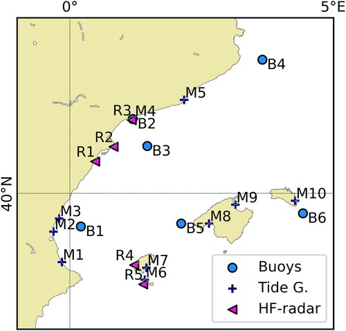
4.1.3. Description of the event

4.1.3.1. Synoptic description of the meteorological situation

Storm Gloria impacted the study area () from 19 to 24 January 2020. A surface low developed over the entire western basin (de Alfonso et al. Citation2021), because of the so-called Rex Block, a large-scale blocking pattern characterised by two adjacent (northern) high and (southern) low pressure systems in upper atmospheric levels (Rex Citation1950). Rather than the relatively deep system of low pressures over the western Mediterranean, the primary source of Gloria was the anomalously powerful anticyclone that governed central Europe, with sea level pressure exceeding 1050 hPa.

This persistent dipole was visible for the whole investigation period, following a clockwise rotation. During the first stage of the developing surface cyclone (19th–20th), an intense pressure gradient gave rise to very strong northeasterly winds (above 20 m·s^–1) that affected broad areas of the eastern coast of Spain. On January 19th and 20th, wind gusts reached 108 km h⁻¹ in Barx (Province of Valencia, Community of Valencia) and 115 km h⁻¹ in Oliva (same province as Barx).

Afterwards, during the 21st, the atmospheric pattern evolved towards a north–south-oriented dipole, triggering a change to predominant easterlies blowing over the entire study area. The dipole-like sea level pressure structure weakened during the 22nd and mostly vanished by the 23rd, with Sea level pressure differences over the region affected by Gloria presenting values similar to pre-storm conditions. The northern high-pressure system fully dissipated by 24 January, while the weakened low remained for a few days at lower latitudes.

This extreme meteorological situation induced a strong response in the ocean, generating extreme values of the main ocean variables as shown in , the details of which will be described in the rest of section 4.4.

Figure 4.1.2. Maximum values recorded during the Gloria event for the different ocean variables. Upper left panel shows significant wave data, upper centre Mean wave period, upper right current speed, lower left sea level residual and lower right high frequency sea level oscillations amplitude. CMEMS data product ref-4.1.5.

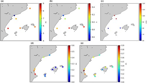
4.1.3.2. Waves

shows the forecasted significant wave height fields provided by the Portus wave model at different times. The figures coincide with the storm peak at Dragonera (a), Valencia (b), Tarragona (c) and Begur (d). The maximum value, over 8 m, was reached in Gulf of Valencia, on January 20th (see the Complementary Material for a description of the temporal evolution).

Figure 4.1.3. Map of the significant wave height field provided by the forecast wave system during Gloria at: 2020-01-20 02 UTC (a), 2020-01-20 06 UTC (b), 2020-01-20 13 UTC (c) and 2020-01-21 00 UTC (d). They coincide with the storm peak measured at Dragonera, Valencia, Tarragona and Begur respectively. Product ref-4.1.7.

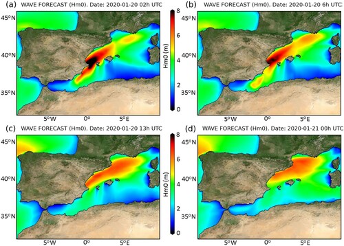
The evolution of the storm is consistent with the magnitude and direction of the wind during the event. These spatial wind fields produced the highest waves () in the region at the north of Cape de la Nao, where the buoy M1 is located (see ). At this position, and for an along-shore wind as generated by Gloria, the whole Catalan-Balear Sea acts as an effective fetch area, explaining the location of the highest wave height observations and the exceptional long wave periods.

New records of significant wave height were observed on five of the six buoys in the region affected by the storm, on occasion with drastic increments (de Alfonso et al. Citation2021). The Valencia buoy’s highest historical measurement increased to 8.4 m (see ) from the previous 6.2 m. The associated mean wave period (Tm02), recorded at the peak of the storm, shows extraordinarily high values. It exceeded 9 s in four of the six locations. These values set new records for the Valencia, Tarragona, Tarragona coastal and Begur buoys. At the Tarragona deep water and coastal buoys, the maximum value for Tm02 arrived some hours after the storm peak, reaching 9.1 and 8.7 s, respectively. This is consistent with previous studies of the region, where the significant wave height (Hm0), peak period (Tp) and duration present a significant interdependence (Lin-Ye et al. Citation2016).

Significant wave heights beat the record for duration. Significant wave height was above 5 m for 39 h, while the usual duration of such high waves is around 12 h. This was a critical factor in Gloria being so destructive. This extraordinary length is linked to the duration of the winds over the area, associated with the slow evolution of the dipole of the pressure gradient and very strong from the 19th to 22nd. Analysis of the wind maps derived from the numerical models shows that most of the Catalan-Balear Sea suffered winds over 15 m s⁻¹ for a period longer of at least 50 h, and winds over 6 m s⁻¹ for three consecutive days (de Alfonso et al. Citation2021). Mean wind regime analysis in the region shows that only around 7% of the storm events have similar durations.Footnote¹

Portus tide gauges measure at 2 Hz frequency, monitoring waves inside the ports. During Gloria, local significant wave height Hm0 reached 2.11 m at Valencia (new historical record), 1.03 m at Gandía, 1.74 m at Tarragona and 1.36 m at Sagunto. Peak periods (Tp) were, as mentioned, very long for the area, reaching 12.89 s at Valencia and 12.68 s at Tarragona. Note that these local measurements depend strongly on the instrument location inside the harbour. Valencia, Tarragona and Sagunto are the most exposed to the open ocean wave conditions (de Alfonso et al. Citation2021). In any case, these high values demonstrate that wave contributions to inundation processes must be considered.

4.1.3.3. Sea level

The largest increase of sea level during Gloria was recorded at Valencia, Gandía, and Sagunto tide gauges, followed by Carboneras and Tarragona (Pérez-Gómez et al. Citation2021). The sea level increase was small or even negligible at the rest of ports (Balearic Islands and Barcelona) (see ), confirmed by the magnitude of the non-tidal residual. De-tiding hourly data, the surge component reached 54 cm above Mean Sea Level (MSL) at Gandía, 47 cm at Valencia, 43 cm at Sagunto, 35 cm at Tarragona and 15 cm at Barcelona. Surge values were <10 cm above MSL in the Balearic Islands (Ibiza, Palma, Alcudia, Mahón, and Formentera). Hourly total sea level achieved an historical record only at Gandía (64 cm), well above the second highest value (59 cm) recorded in 2010 (time series 2007–2020), while in Valencia and Sagunto the maximum hourly value was the third highest since 2007. Interestingly, in Barcelona, the maximum reached only 55 cm above the tide gauge datum, far from the historical records at this harbour (81.2 cm in 2019). Sea level was over the 99th percentile for at least two days at Gandía, Valencia and Sagunto.

This behaviour of sea level is consistent both with the wind fields and the current fields (see ). Theory states that the vertically integrated wind-induced transport in shelf areas tends to be more aligned with the wind than in open waters (where it is expected to be perpendicular, following Ekman’s theory), due to the effect of the bottom spiral (Pugh Citation1996). As a result, the wind piled water in all the coastal domain south of Ebro’s Delta, but particularly against Cabo de la Nao (at the M1 sea level gauge region), which became a natural barrier for water transport explaining, the maximum amplitude measured at Gandía. This also explains the much smaller surge at Barcelona and at the Balearic Islands (see ).

Apart from waves and hourly sea level, it was found that High Frequency Sea Level Oscillations (HFSLO), with periods within 30–300 s, had significant magnitude and were relevant for understanding coastal damages (Pérez-Gómez et al. Citation2021). Again, the Portus high frequency sampling makes such an assessment possible. Maximum HFSLO amplitude (Hmax: maximum oscillation amplitude in one hour) reached record values for the period since the installation of the new radar sensors in Valencia (90 cm), Sagunto (57 cm) and Ibiza (60 cm). Gandía and Tarragona recorded their 5th highest maximum Hmax in their time series.

Spectral analysis of the time series shows that, during this event, the HFSLO energy was mainly concentrated in the infragravity band (30–300 s). The well-known origin of these oscillations, very frequent on the Iberian Peninsula Atlantic coast, but unnoticed before on the Mediterranean one, is transfer of energy from long period waves. This is reinforced by two facts: (1) in all cases, the energy evolution of the 30–300 s band is highly correlated in time with the height of the waves measured by the tide gauges and (2) there is a clear correlation between the presence of long wave periods and activity in the infragravity band (see ).

Figure 4.1.4. Infragravity band energy (30 s – 5 min band) at the tide gauge vs T_m02 at the closest buoy for the historical tide gauges record. The historical maximum energy in this band was recorded in Valencia, Sagunto and Ibiza during Gloria (circles). Colour code represents the significant wave height. All data from product ref-4.1.5., except 2 Hz data from ref-4.1.7.

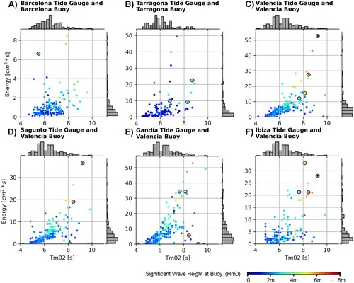
4.1.3.4. Currents

The circulation models illustrate the impact on the currents of the shelf region (see with results from the WMOP system). The winds created a strong along-shore current in the region, affecting mainly the shelf and, to a lesser extent, the slope. This pattern induced a transport that is consistent with the areas of maximum surge, as shown in . Nevertheless, the model information about the values of the currents at a specific point and time cannot be given with the same reliability as is the case for the waves, as will be shown in the validations presented as complementary material.

Figure 4.1.5. Daily average WMOP surface currents (cm/s) for the pre-storm (18 January 2020), storm (20 January 2020) and post-storm (23 January 2020) conditions. The arrows and the colour indicate the direction and the magnitude of the currents, respectively. Data product 4.1.6.

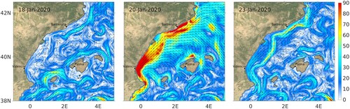
The Ebro delta region is monitored by a buoy (B3 in ) with a current meter, and by HF radar stations (R1, R2 and R3 in ). Results of both systems can be seen in . Both the HF-radar system and the deep-water buoys measured high values of sea current magnitude in the region, as a clear response to the wind. The impact of Gloria is evident on the surface maps obtained by the HF-radar (see , upper panels). Before the arrival of Gloria, the Ligurian-Provençal-Catalan current is visible, but with moderate velocity. Observations during the event show both a perceptible intensification of the surface currents and a broadening of the strong current area, as a direct response to the intense winds. These observations are consistent with the model results shown in (see complementary material section for further considerations on the model performance).

Figure 4.1.6. Upper panel shows the observations of the HF radar during Gloria event (daily means). Lower panels the comparison of hourly surface current speed (A) and direction (B) provided by B3 buoy (red) and HF radar (blue) at the closest grid point, for January 2020. CMEMS data product ref-4.1.5.

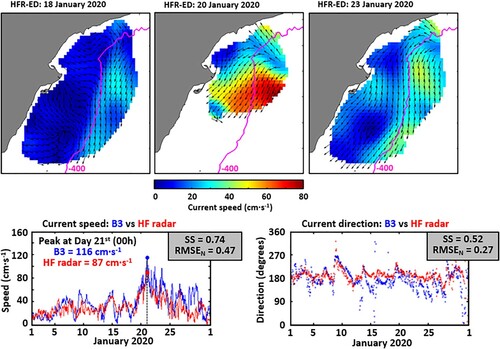
It is remarkable that at the position near Valencia, where the B1 buoy is located, the currents generated by the model are confined to the shelf. This explains the relatively low maximum velocities observed at this position (), since the buoy is located at the shelf break. In any case, as will be shown in the annex on models validation, the details of the solution for currents provided by the numerical models at a specific point at time must be considered with caution.

Hourly B3 buoy time series of current speed and direction were compared with HF radar data estimations at the closest grid point (see , lower panels). Both devices captured the timing of the peak in the current speed (January 21st at 00 h), although the HF-radar undermeasured the exceptional value recorded by the Tarragona deep water buoy (116 cm s⁻¹). This measurement is over the 99.9 percentile and the 15-year historical record, previously established at 79 and 98 cm/s, respectively. Note that the highest current speed registered during another severe event in January 2017 was 53 cm.s⁻¹ (half of Gloria event´s top speed), highlighting the exceptionality of Gloria.

Additionally, Gloria's effect in an adjacent area, less affected by the event as evidenced by the model results, could be seen on the anomalous surface circulation patterns measured by the HFR systems in the Ibiza Channel (R4 and R5 on ). On the 19th of January, the analysis of the HFR derived surface currents in the Ibiza Channel revealed the intensification of the surface flow (reaching 60 cm/s), with a clockwise veering from NE to SW during the storm, abruptly interrupting the well-known Balearic current (Lorente et al. Citation2021).

4.1.4. Discussion

The spatial coverage and temporal sampling of the ocean observing system has been exploited to monitor the impacts of the Gloria event, except in the case of the HF radar. For the latter, the low number of stations only permits monitoring of surface currents for limited regions. All available instrumentation produced timely critical data. This is a result of best practices applied on the maintenance of these instruments. Nevertheless, it is important to highlight that this is not the case for all storms. On some occasions, instrumentation is under maintenance or repair. The deep-water buoys of Puertos del Estado employed in this paper are typically available 90% of the time during a normal year. Looking at it is obvious that the level of spatial redundancy of the system is low, and this could have consequences. For example, one of the most important reasons to measure waves is for obtaining long time series that can be used for extreme analysis, something mandatory when designing maritime infrastructures, such as piers. Note that the cost of these public works range typically from tens to hundreds of millions of Euros. The impact of Gloria on these works is clear when computing return periods. For instance, in Valencia, the Hm0 of 8.44 m was associated with a return period of 707.7 years before Gloria but is reduced to 37.2 years when considering the new data. Similarly, in Dragonera, the Hm0 of 7.97 m (544.4 years) has changed to a new return period of 40.3 years, whereas in Tarragona, a Hm0 of 7.62 m (414.7 years) corresponds to a new return period of 48.7 years. This demonstrated that losing the data from one storm due to a malfunction of an instrument can have important consequences when designing new infrastructures, something that will affect both their construction cost and safety. Obviously, numerical modelling came as a help here to fill the gaps, but considering the costs associated with the creation and repair of coastal infrastructures, it is valuable to have reliable measurements. Additionally, a higher level of redundancy would contribute to reduce gaps in the data and, therefore, to help in the study of trends of extremes in climate change studies. Therefore, more stress should be placed in the future on the redundancy of instrumentation, even if the maintenance costs are increased.

All the forecasts and measurements were distributed to the community through the Portus web page (product ref-4.1.7.) and, in the case of the Ports, via the specific SAMOA (Sistema de Apoyo Meteorológico y Oceanográfico a las Autoridades Portuarias) service, a series of downscaled models and downstream applications designed to provide the information required for safe Port operation (Alvarez-Fanjul et al. Citation2018). Thanks to this information, all major Ports at Spain in the affected area took contingency actions, like closing to maritime traffic in advance, reducing the possibilities of fatal accidents. A good example of these preventive actions can be found at Barcelona Port. At this location, the SAMOA service includes an overtopping forecast service. The first overtopping alert was issued on 16 January 2020 12 h (72 h forecast), and the last overtopping alert was on 23 January 2020 00 h (12 h forecast). The overtopping was successfully predicted, with an error below 3 h of the first recorded event, within 72 h of anticipation. This gave time to the Port Police to close certain areas of the pier to pedestrians and road traffic, preventing possible accidents. It is noteworthy that the forecast horizon of 72 h was sufficient to implement mitigation actions. Real time validation of the models, based on the Portus observing component, was also important to generate confidence in the forecasting systems. During the event, and in the previous days, the real time validation system was critical to increase the confidence of the stakeholders at the Ports that, alarmed by the unprecedent forecasts, contacted Puertos del Estado, seeking additional confirmation.

Finally, the observations of the Portus system are demonstrating that climate change is also playing its role in the devastation. According to the relative mean sea level trends obtained from Barcelona, Valencia and Ports, the overall relative sea level rise in 27 years may have reached up to 15 cm at some coastal locations of the Spanish Mediterranean coast. Over this higher mean sea level, all relevant sea level oscillations discussed here have taken place. In simpler words, the same surge magnitude would generate total extreme sea levels up to 15 cm higher today than in 1993.

In summary, this study has illustrated that local operational oceanography services in the area, providing integrated information with CMEMS services, are ready to generate useful information for decision making during extreme events. The coastal damages and human life losses produced by Gloria highlight the importance of investing in a state-of-the-art monitoring and forecasting system. In this case, international collaboration at the European level was of paramount importance, and thanks to the CMEMS service, several aspects of the storm were properly forecast, and mitigation actions were taken in advance.

Section 4.2. Oceanic response to the 2020 Siberian heatwave

Authors: V. S. Lien, S. Aaboe, E. J. Down, L. Bertino, S. Hendricks, T. Lavergne, J. Xie, A. Mangin, M. Bretagnon

Statement of main outcome: 2020 stands out as one of the years with the least sea ice in the Arctic since satellite records started in the late 1970s. For each of the months July to December, the sea-ice cover was either at its lowest or second lowest on record. Most remarkable was the one month earlier melting and one-month later freeze-up in the Kara and Laptev seas, giving rise to prolonged ice-free seas along the Siberian shelf. The sea-ice anomalies followed the record-breaking heatwave in northern Siberia. We find that anomalous, wind-driven sea-ice drift in the Laptev Sea basin in July 2020, preconditioned by anomalously thin sea ice, exposed the ocean to prolonged heating from incoming shortwave radiation. Moreover, higher surface salinities in the Laptev Sea basin due to the lack of local ice melt, combined with large SST anomalies and subsequent vertical mixing, reduced the upper 100 m water column stability by more than 50% compared with the climatological average. Consequently, 2020 has experienced a positive anomaly in primary production in the Arctic shelf regions, due to the relatively higher supply in nutrients within the surface layer, and a decrease for the global Arctic By December, the sea-ice thickness in the Laptev Sea increased to climatological values through a combination of freezing and regional convergence. Below the sea-ice cover, a reduced stability persisted in the upper 100 m of the water column.

Products used:

Table

4.2.1. Introduction

The Arctic climate is undergoing warming that is unprecedented in the historical record (e.g. Polyakov et al. Citation2012; Polyakov, Bhatt, et al. Citation2013; IPCC Citation2019; Overland et al. Citation2019), that, among other things, has been manifested in a shrinking sea-ice cover (Serreze et al. Citation2007; Comiso et al. Citation2017; Onarheim et al. Citation2018; Landrum and Holland Citation2020). This reduction in sea-ice cover induces positive feedback mechanisms through increased coupling between wind, sea ice and surface currents (e.g. Alkama et al. Citation2020; Polyakov, Rippeth, Fer, Baumann, et al. Citation2020). The result is more energetic inertial oscillations and a weakening of the cold halocline of the Arctic Ocean leading to enhanced ventilation and increased vertical heat fluxes, as well as a shoaling of the underlying warm and saline Atlantic Water (e.g. Polyakov et al. Citation2017; Polyakov, Rippeth, Fer, Alkire, et al. Citation2020; Polyakov, Rippeth, Fer, Baumann, et al. Citation2020; Aaboe et al. Citation2021). Subsequently, the increased vertical heat fluxes lead to delayed and reduced sea-ice growth (e.g. Polyakov, Pnyushkov, et al. Citation2013; Ivanov et al. Citation2016; Polyakov, Rippeth, Fer, Alkire, et al. Citation2020). Moreover, the decreased sea-ice cover allows for more absorption of shortwave radiation, increasing further the heat content of the surface layer and thus delaying the re-freeze and extending the ice-free season (e.g. Serreze et al. Citation2009; Stroeve and Notz Citation2018). As the primary production in the water column is controlled by nutrients and light availability, an extended sea-ice free season may foster primary production (Arrigo and van Dijken Citation2015). Primary production is further regulated by the water column stratification that limits the upward fluxes of nutrient rich water into the surface layer and by inflow of nutrients into the Arctic Ocean from adjacent seas (Lewis et al. Citation2020). The biological carbon pump may be affected by the modifications in primary production amplitude and induce positive or negative feedback mechanisms on climate change.

An exceptional warm event occurred over Siberia in 2020, with monthly air temperature anomalies exceeding 5°C. The event was caused by an anomalously strong stratospheric polar vortex and tropospheric jet stream (ESOTC Citation2020; Overland and Wang Citation2020). Moreover, the temperature anomalies were 2–3 degrees Celsius warmer than during comparable anomalies in the stratospheric polar vortex in 1989 and 1990 due to Arctic amplification (Ciavarella et al. Citation2021; Overland and Wang Citation2020). While the stratospheric polar vortex weakened in May, southwesterly winds carried warm air towards the Siberian coast in June (Overland and Wang Citation2020).

Subsequent to the extreme heat wave, the extent of the Arctic sea ice was remarkably low in 2020 with monthly record-lows in July and October and monthly ice extents from April to December were individually among the lowest four on record for each month, according to the OSI SAF Sea Ice Index (v2.1, Citation2020) which is based on product 4.2.1. Most striking was the vast ice loss along the Siberian coast with the record-low and rapid break-up of sea ice in the Laptev Sea starting approximately one month earlier than the 2010–2019 average and the extraordinary late freeze-up in the Kara and Laptev seas, giving rise to prolonged ice-free seas along the entire Siberian shelf regions (, bottom; ESOTC Citation2020).

Here, we provide analyses of the ocean and cryosphere states following the Siberian heat wave in 2020, based on both numerical ocean model simulations and satellite remote sensing products.

4.2.2. Data and methods

In this contribution, we mainly present monthly averaged fields and their corresponding monthly anomalies relative to the reference period of 2010–2019 (referred to in the following as ‘reference period’). The products used are presented below.

The sea-ice properties have been monitored with satellite remote sensing since the 1970s. The Ocean and Sea Ice Satellite Application Facility (OSI SAF) global sea-ice concentration climate data record (product 4.2.1, Lavergne et al. Citation2019) is computed from the long series of passive microwave radiometers (SMMR, SSM/I, and SSMIS) and covers the period from 1979 to present. From the concentration data, we derive the regional sea-ice extent for the Laptev Sea defined within the region of 70–80°N and 100–145°E (see grey box outlined in (A)). The sea-ice extent is computed as the cumulative ocean surface covered by at least 15% sea-ice concentration.

Figure 4.2.1. Arctic Ocean sea-ice conditions (concentration, thickness, and drift) in selected months during 2020. In the left column is shown the monthly averaged sea-ice values and in the right column is shown the monthly anomalies of each of the sea-ice properties with respect to the reference period 2010–2019. In the left column, the SST anomaly (red-blue scale, product 4.2.4) is included over the ice-free regions. (A, B) Sea-ice concentration (greyscale, product 4.2.1) with sea-ice drift (arrows, product 4.2.2) superimposed, July 2020. (C, D) Same as (A, B), but for September 2020. (E, F) Sea-ice drift (product 4.2.2) on top of the sea-ice thickness (blue scale, product 4.2.3), October 2020. (G, H) Same as (E, F), but for December 2020. The grey box indicates the Laptev Sea region for computation of the sea-ice extent index in . The grey line indicates the position of the Laptev transect for .

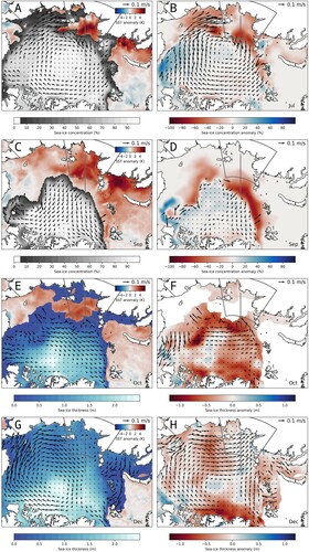
The OSI SAF sea-ice drift near-real-time product (product 4.2.2) is a multi-sensor product based on passive microwave and scatterometer measurements and has been operational since the end of 2009 (Lavergne et al. Citation2010).

The sea-ice thickness (SIT) data record is based on merged radar altimeter data from CryoSat-2 and L-Band passive microwave measurements from SMOS (Ricker et al. Citation2017) in the winter months of October through April since November 2010 (provided by Copernicus Marine Service (CMEMS), product 4.2.3). The SIT information is based on optimal interpolation of SIT fields from the two methods with an observation period of 7 days and contains gap-less SIT information on a 25 km grid.

The Operational Sea Surface Temperature and Ice Analysis (OSTIA) system is run by the UK's Met Office. The OSTIA data (product 4.2.4) is a Level-4 interpolated product from multiple sensors (Good et al. Citation2020). The same product has been used for 2020 and for the reference period 2010–2019. OSTIA uses satellite data provided by the GHRSST project together with in-situ observations to determine the sea surface temperature. A high resolution (1/20° – approx. 6 km) daily analysis of sea surface temperature (SST) is produced for the global ocean.

The Arctic Monitoring and Forecasting Center (Arc MFC) model is the TOPAZ4 system based on a North Atlantic and Arctic configuration of the HYCOM ocean model coupled to a modified version of the CICE3 sea-ice model at a horizontal resolution of 12 km, assimilating various ocean and sea-ice observations once a week, including sea-ice concentrations from OSI SAF and ice thickness from the merged CS2SMOS product (since 2014) with an Ensemble Kalman Filter (Xie et al. Citation2016). The model data for the reference period are based on the Arc MFC re-analysis (product 4.2.5), while the best-estimate output from the analysis and forecast, the average of a 100-members ensemble, is used for 2020 (product 4.2.6). For further information about the model system and data assimilation, see Sakov et al. (Citation2012).

Based on Arc MFC outputs, we compute the mixed-layer depth (MLD) by applying the threshold method (e.g. Peters et al. Citation1989). Defining the potential density difference, Δσ_Θ, between the surface z₀ and the depth z as: (1) $Δ σ_{Θ} (z) = σ_{Θ} (z) - σ_{Θ} (z_{0})$ (1) the MLD is defined as the depth z at which Δσ_Θ exceeds a specified threshold value, here set to Δσ_Θ = 0.03 kg m⁻³, (2) $MLD : Δ σ_{Θ} (MLD) = 0.03 kg m^{- 3}$ (2)

In order to analyse the stability of the water column, we have estimated the Brunt-Väisälä frequency, N, by calculating N² following the equation: (3) $N^{2} = \frac{- g}{ρ_{0}} \frac{δ ρ (z)}{δ z}$ (3) where g is the gravitational constant, ρ is the density of seawater, ρ₀ is the density of the surface layer, and z is the depth. The higher values of N² represent a stronger water column stratification.

The modelled oceanographic results are shown for a section crossing the Laptev Sea and into the Eurasian basin between (74.13°N, 127.33°E–84.42°N, 112.56°E), see outline in . In the following this section is referred to as the ‘Laptev transect’. Our motivation for studying this specific section is to focus on the area of the largest sea-ice anomalies during the melting season (). Moreover, the section was found to be representative of the anomalous oceanographic conditions in the central Laptev Sea in summer 2020 (). A comparison with a CTD transect obtained in the same area in 2015 and 2018 under the NABOS-project (Nansen and Amundsen Basins Observational System, https://uaf-iarc.org/nabos/) showed that the modelled hydrography in the surface and halocline layers compared fairly well with observations. The mixed-layer depth, however, tended to be somewhat deeper in the model (around 20 m) compared to 10–20 m in the observations. More general and weekly updated validation of the model results against observations are available at https://cmems.met.no/ARC-MFC/V2Validation/index.html. Specifically, the model and the observations agreed with respect to the type of sea ice present in the Laptev Sea in April 2020, and the average sea-ice thickness bias in the model was close to zero, with an RMS difference of 0.3 m, when comparing with SMOS thin-ice thickness data (i.e. areas where sea-ice thickness is less than 1 m). The reason for comparing model and SMOS data in April is the lack of availability of SMOS data in May–September (see above). The weekly model validation also shows that modelled sea-ice drift is generally in good agreement with the observations, both in terms of magnitude and direction.

Figure 4.2.2. (A) Modelled sea-ice thickness anomalies in June 2020 (in standard deviations from the reference period 2010–2019), based on product 4.2.5 (2010–2019) and 4.2.6 (2020). (B) 10 m wind divergence (colour) and wind speed and direction (arrows) in July 2020, from ERA5. (C) Net downward shortwave radiation anomaly in July 2020 relative to the reference period 2010–2019 (in standard deviations), from ERA5. (D) Modelled surface layer salinity anomaly in August 2020 relative to the reference period 2010–2019, based on product 4.2.5 (2010–2019) and product 4.2.6 (2020). Grey box shows the area used to calculate the sea-ice extent index in (). Grey line shows the Laptev transect.

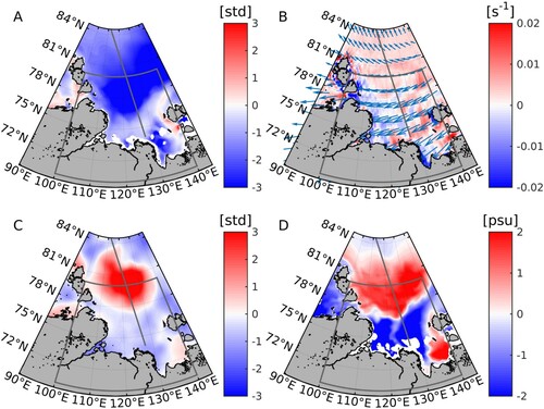
Wind divergence based on monthly averaged U- and V-10 m winds and hourly net surface shortwave radiation obtained from the ERA5 reanalysis (Hersbach et al. Citation2020) were also included.

In addition to physical properties, remote sensing observations allow us to investigate biological activity. Based on the work by Antoine and Morel (Citation1996), primary production is estimated from ocean colour data (chlorophyll concentration and photosynthetically available radiation) and sea surface temperature. These observations at a spatial resolution of 4 km give a full coverage of the region of interest on a monthly basis. Note that primary production evolution can only be assessed from May to September, since the polar night prevents satellite passive optical sensor observations. Satellite observations of primary production above 80°N are also limited by the sun's low zenith angle.

4.2.3. Results and discussion

The anomalous sea-ice conditions in 2020 were observed together with extraordinary warm surface temperatures in the Arctic region as a whole () but especially they followed the exceptionally strong and long-lasting atmospheric heat wave in the Arctic Siberia in spring/early summer and autumn (ESOTC Citation2020). (A and C) show the monthly sea-ice concentration combined with monthly SST anomalies over open water (less than 5% ice concentration) for July and September, respectively. The SST anomalies exceeded 4 degrees in the Kara Sea to the Laptev Sea and a thousand kilometres off the Siberian coastline. The corresponding monthly sea-ice anomalies are given in (B and D), showing coincident regions with warm SST anomalies and reduced sea-ice cover. Already by the end of July the whole area of the Laptev Sea was virtually ice free ( and ).

Unfortunately, no remote sensing estimates exist for sea-ice thickness during the summer months. However, in April (not shown), before the summer melting, the sea ice was generally thinner relative to the reference period on the Siberian shelves east of the Kara Sea (i.e. including the Laptev Sea). Moreover, the model results show that the sea ice got progressively thinner compared to the reference period, from March through June (sea-ice thickness anomalies in June are shown in (A)). This coincides with the findings of Overland and Wang (Citation2020), who reported a northward advection of the Siberian heatwave to the Siberian shelves in June, but with noticeable warm temperature anomalies also over the Laptev Sea from April and onwards (Figure 1 in Overland and Wang Citation2020). On average, the sea ice was between 0.5 and 1 m thinner in large parts of the Laptev Sea in June, which corresponds to more than 3 standard deviations below the reference period average ((A)). This preconditioned the sea-ice cover to be more susceptible to wind-driven sea-ice drift during the following melting season. In October, the remotely sensed ice thickness showed a negative anomaly dominating most of the Arctic Ocean with strong thickness reductions north of Greenland and toward Siberia ((F)). The same pattern of negative thickness anomaly is present in November (not shown) and partly in December, but in December a noticeable positive thickness anomaly developed in the Laptev Sea together with strong anomalous on-shore ice drift ((H)). The monthly averaged ice drift in December is relatively weak in the Laptev Sea ((G)) meaning that the strong on-shore drift anomaly rather represents a weaker or absent off-shore drift in 2020 compared to the reference period.

In July, during the summer melting period, the wind field over the northern Laptev Sea (i.e. deeper basin part) was divergent (e.g. ESOTC [Citation2020], ‘Arctic sea ice’) with anomalous northerly (i.e. off-shore) winds ((B)). This resulted in stronger northward sea-ice drift toward the central Arctic in 2020 relative to the reference period ((A–D)). Consequently, less sea ice melted locally in the central Laptev Sea during the summer months. With strongly reduced ice cover, the net downward shortwave radiation in the central Laptev Sea in July was more than 3 standard deviations (>15 W/m2) above the reference period mean ((C)). In the following, we discuss the oceanic response to the anomalous sea-ice conditions during summer 2020, utilising the results from the Arc MFC model.

The modelled density in the Laptev transect revealed positive anomalies mostly confined to the upper 100 m in the region between 77°N and 82°N, which corresponds to the offshore, deep basin part of the Laptev Sea (see ). Within the mixed layer the anomalies exceeded 1 kg/m³ relative to the reference period, and were the strongest around September (, left). The density anomalies were caused by anomalously high salinities in 2020, especially within the surface mixed layer. Indeed, looking at the water mass characteristics in a Θ-S diagram revealed that the salinity of the surface layer was higher in June 2020 than in the reference period. Moreover, in 2020 the surface salinity remained more or less constant from June through August, as opposed to declining in the reference period (, inset). Over the same period, the surface temperature increased in 2020 from being close to the freezing point in June to nearly 3°C in August/September. The temperature increase extended, to some degree, below the MLD, as did also the salinity anomalies (). However, due to the dominant role of the salinity in determining the density at these low temperatures, the effect from the temperature increase (contributing to a density decrease) was small compared with the effect from the salinity increase (causing density increase), or rather a lack of salinity decrease, relative to the reference period (, inset). While we acknowledge that the above results are based on a vertical transect across the Laptev Sea, we note that the transect is representative for the conditions in the deep-basin part of the Laptev Sea during summer 2020 ((A–D)). Clearly, the positive sea-surface salinity anomaly developed locally within the Laptev Sea ((D)). Moreover, previous observations indicate advection speeds of only a few centimetres per second in this area (e.g. Pnyushkov et al. Citation2021). Hence, any advected hydrographic anomalies would require an advection time from the upstream Kara Sea to the Laptev Sea of several months.

Figure 4.2.3. Monthly density anomalies (kg/m³, product 4.2.6 for 2020 values and product 4.2.5 for the reference period) in the Laptev transect, for September (A) and December (B). See transect location outlined in . Thin black and red lines show the monthly MLD (Equation 2) for the reference period (2010–2019) and in 2020, respectively. The thick, broken line at the surface represents the sea-ice extent (in the model defined as sea-ice concentration > 30%); black when ice occurred both in 2020 and in the reference period, and red when ice occurred in the reference period but not in 2020.

Figure 4.2.3. Monthly density anomalies (kg/m3, product 4.2.6 for 2020 values and product 4.2.5 for the reference period) in the Laptev transect, for September (A) and December (B). See transect location outlined in Figures 4.2.1 and 4.2.2. Thin black and red lines show the monthly MLD (Equation 2) for the reference period (2010–2019) and in 2020, respectively. The thick, broken line at the surface represents the sea-ice extent (in the model defined as sea-ice concentration > 30%); black when ice occurred both in 2020 and in the reference period, and red when ice occurred in the reference period but not in 2020.

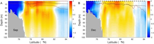
Figure 4.2.4. Top: Modelled monthly Brunt-Väisälä frequency (N², Equation 3), potential temperature Θ and salinity S using the surface layer and the 100 m depth averaged over the region of 78°N–81°N in the Laptev transect (see outline in ). Blue line shows the reference average (2010–2019; product 4.2.5). Red line shows the values in 2020 (product 4.2.6). Insets: Average Θ-S properties in the surface layer (stars) and at 100 m depth (triangles) during the reference period (blue) and in 2020 (red). Bottom: Observed daily sea-ice extent in the Laptev Sea as a fraction of the total Laptev area; red represents the sea ice in 2020 and blue represents the averaged sea-ice extent in the reference period 2010–2019 (blue). Based on data from OSI SAF climate data record (product 4.2.1). Note, that the ticks on the x-axis represent the midpoint of the month.

$Figure 4.2.4. Top: Modelled monthly Brunt-Väisälä frequency (N2, Equation 3), potential temperature Θ and salinity S using the surface layer and the 100 m depth averaged over the region of 78°N–81°N in the Laptev transect (see outline in Figure 4.2.1). Blue line shows the reference average (2010–2019; product 4.2.5). Red line shows the values in 2020 (product 4.2.6). Insets: Average Θ-S properties in the surface layer (stars) and at 100 m depth (triangles) during the reference period (blue) and in 2020 (red). Bottom: Observed daily sea-ice extent in the Laptev Sea as a fraction of the total Laptev area; red represents the sea ice in 2020 and blue represents the averaged sea-ice extent in the reference period 2010–2019 (blue). Based on data from OSI SAF climate data record (product 4.2.1). Note, that the ticks on the x-axis represent the midpoint of the month.$

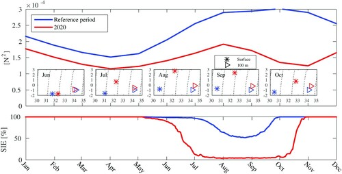
In contrast to the positive density anomaly seen in the offshore part of the Laptev Sea in 2020, there was a strong, negative density anomaly over the shelf region (). Again, this was caused by a salinity anomaly, here being negative (not shown). The model results suggest that a freshwater anomaly was present on the shelf already in January 2020 (not shown), i.e. prior to the warm surface air temperature anomaly starting in winter/spring 2020. Since the offshore saline water was not propagating onto the shelf, the density front between the shelf and deep basin instead intensified during 2020 (). In the following, the focus is on the offshore conditions (i.e. north of 77°N).

Further analysis of the stability of the water column in 2020 relative to the reference period showed that 2020 had a generally weaker stratification of the upper 100 m with lower values of the Brunt-Väisälä frequency (N²) based on modelled density in the surface layer and at 100 m depth (Equation 3, ). This result was qualitatively robust using other integration depths, such as e.g. 200 m. Despite the lower values of N² in 2020, it still followed a similar seasonal cycle as for the reference period from January to August with a minimum in April. This minimum is related to the end of the sea-ice growth season and the associated input of salt from sea-ice freezing and subsequent brine rejection at the surface. As the melting season reached its maximum in June and July, the stability increased, but less so in 2020 compared with the reference average. In the reference period, the stability increase was largely due to a decrease in the surface salinity, whereas in 2020, the stability increase was largely due to increased temperature in the surface layer, in addition to a salinity increase deeper below (, inset). The lack of a stabilising fresher surface layer in 2020 was most likely due to a combination of the thinner sea ice and the increased advection of sea ice out of the region during the melting season ((A)). The salinity was also anomalously high at 100 m depth. One explanation for this increased sub-surface salinity could be upwelling related to the increased divergent wind pattern in July 2020. However, exploring this in more detail is beyond the scope of this paper. Moreover, a deepening of the MLD, as discussed below, could also play a role in contributing to the weaker stability increase in 2020.

From August through October 2020, there was a diverging pattern in the upper water column stability from the reference period (). In 2020, the stability decreased towards a minimum in November due to increasing salinity in the surface layer during September to November (, inset), whereas for the reference average, the stability increased throughout August and then remained more or less stable through October before it started decreasing. Indeed, the stability of the upper 100 m in November 2020 was comparable to the minimum for April 2020 and less than 50% of the reference period average. From early August to late October the Laptev Sea was virtually open water () and there was no ice formation until late October/early November. Thus, the only source of salt to increase the salinity of the surface layer in the period August through October would be upward mixing of more saline water from below. A possible explanation for the decreasing water column stability from August to November is therefore enhanced vertical mixing due to the prolonged timespan of open water. This is in agreement with the findings of Polyakov et al. (Citation2017), Polyakov, Rippeth, Fer, Alkire, et al. (Citation2020), Polyakov, Rippeth, Fer, Baumann, et al. (Citation2020), that a reduced sea-ice cover in the Arctic enhances the vertical mixing, which erodes the cold halocline and the associated upper water column stability.

Exploring in more detail possible explanations for the positive surface salinity anomaly during the melting season in 2020 (i.e. June through August), we investigate the modelled sea-ice melt along the Laptev transect to substantiate the observed anomalous sea-ice drift and negative sea-ice thickness anomaly in the Laptev Sea (). From the model results, we find that the cumulative sea-ice melt during the melting season in the reference period (between 78°N and 81°N) provided freshwater sufficient to reduce the salinity of the upper-mixed layer by around 1 in this region (not shown). This is comparable to the modelled reduction of around 1 (from 31.5 in June to 30.5 in August) in the surface layer in the reference period (, inset). In the summer of 2020, however, the MLD in this region was more than twice the average MLD for the reference period (a subsequent comparison in September is shown in ). Assuming that all the freshwater from sea-ice melt is contained within the mixed layer, the reduced amount of available meltwater in 2020 distributed throughout a deeper surface mixed layer in 2020 could cause a reduced freshening of the surface layer. Thus, the model results indicate that the cause of the 2020 positive surface salinity anomaly, and, thus, density anomaly in the surface mixed layer during the melting season was a combination of a deepening of the MLD and reduced amounts of freshwater from sea-ice melt.

From a biological point of view, the primary production within the coastal regions of the Arctic Ocean accounts for a significant proportion of the total primary production. For instance, in 2020, while the average of primary production over the whole region reached 260 mgC.m^–2.d^–1, the coastal region is characterised by an average of 328 mgC.m^–2.d^–1, and the offshore region by an average of 230 mgC.m^–2.d^–1. The physical modifications of the Arctic environment in 2020 resulted in a modification of the biological activity where the coastal regions were more productive during June to September 2020 than during the reference period (). This contrasts the conditions averaged over the entire Arctic region, summer 2020 (between June and September), which was characterised by a decrease of about 5% in primary production compared to the reference period. This offshore decrease in primary production can likely be attributed to the loss in stability. The negative anomaly in primary production for 2020 was however less intense than the one observed for the chlorophyll concentration, for which the anomaly reached −10% during summer 2020. The intensity of the biological productivity is governed by the nutrients and the light availability. The difference in chlorophyll and primary production anomalies can be explained by the non-linear relationship between both parameters and the importance of temperature on the phytoplankton growth.

Figure 4.2.5. Northern Hemisphere primary production during 2020, with monthly estimates (in mgC.m-2.d-1, left column) and monthly anomalies with respect to reference period 2010–2019 (in %, right column). Observations are given for (a, d) July, (b, e) September, and (c, f) October. White region represents the polar data gap due to glint or sun zenith angle.

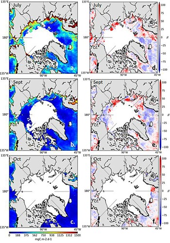
If one considers the whole area, remote sensing observations do not exhibit any significant increase in wind speed nor decrease in photosynthetically available radiation (not shown). This would point out the importance of the water column stability. A modification in water column stability will affect the primary production as a decrease in stability will induce a reduced light availability for the phytoplankton growth. The modification of the stratification of the water column in 2020 will therefore impact the production.

Regionally, the highest primary production anomalies in 2020 are observed from Svalbard toward the Laptev Sea, with primary production being about 80% higher than the reference period ((d, e)). Conversely, in the eastern part of the Laptev Sea and in the Eastern Siberian Sea, the anomalies in primary production are negative (about 25%). Regional positive anomalies in primary production for 2020 can be explained by the warming of the surface layer, as the primary production anomaly pattern appears to be in line with SST anomalies ().

4.2.4. Concluding remarks

In 2020, the eastern Arctic Ocean hosted both extreme air and ocean surface temperatures, record-low sea-ice cover and an ice-free ocean surface exposed to atmospheric influence during a prolonged summer period. Most of the Laptev Sea was ice-free by mid-July and remained ice-free until the end of October 2020, representing a one-month earlier melt season as well as a one-month delay in re-freezing, totalling three months of ice-free conditions (). Satellite remote sensing data and model results also show that the sea ice was thinner than the 2010–2019 average, both in advance of the summer melt and after the Laptev Sea had re-frozen in November (). During spring, the sea ice got progressively thinner compared to the reference 2010–2019 average, preconditioning the sea-ice cover by making it more susceptible to wind-driven advection. In July, a divergent wind field caused anomalous northward sea-ice drift, which contributed to making the Laptev Sea ice-free as early as July. The subsequent anomalously high SST and surface salinity inhibited a re-freeze until the start of November. In December, however, the sea-ice thickness almost recovered to the 2010–2019 average. The surface expression of the anomalous conditions in the Laptev Sea in 2020 was thus lost by December (). However, the elevated salinity in the upper ocean, which caused a reduced upper-ocean stability, persisted ( and ). A weaker upper-ocean stability was found in April 2020 (compared to the reference period) before the Siberian heatwave set in, which can be related to the recently observed increased vertical mixing in the Arctic, as reported by, e.g. Polyakov, Rippeth, Fer, Alkire, et al. (Citation2020). Moreover, we found that the upper-ocean stability in 2020 was even lower at the end of the year (December) than in the beginning (January), indicating a further erosion of the cold halocline during the heat event. Furthermore, we found indications that these modifications of the physical environment affected the biology, characterised by a decrease in chlorophyll concentration of 10% and a decrease in primary production of 5%.

Section 4.3. Monitoring and predictions of the series of marine heatwave events impacting the Northeast Pacific in 2020

Authors: Eric de Boisseson, Magdalena Balmaseda, Michael Mayer, Hao Zuo

Statement of Main Outcome: A marine heatwave (MHW) is defined as a prolonged period (usually 5 days or more) of sea-surface temperature (SST) above the 90th climatological percentile, which is potentially devastating for marine ecosystems and economy. The available ocean information by marine and climate services allows the real-time detection and seasonal prediction of MHW. Reported 2020 MHW events in the North East Pacific happen in the context of increased frequency of long heatwaves. A positive feedback loop by which atmospheric conditions impact the upper ocean stratification making the ocean mixed layer more responsive to anomalous surface fluxes has been identified. The increased stratification at the base of the mixed layer seen since 2017 coincides with the resurgence of MHWs from 2018 onwards. Reliable predictions of developing MHW conditions could help advance planning and preparedness for such extreme variability events in the ocean. The ECMWF SEAS5 system showed skill in predicting the 2020 events at seasonal timescales, especially once the ocean was preconditioned after the first MHW of that year. The first order assessment of SEAS5 skill for MHW predictions presented here showed encouraging results, but for such information to be actionable in the future there is need to gain more confidence on the quality of the seasonal forecast information. Statistical forecast reliability quantification and further process understanding will be the subject of a follow-up study.

Products used:

Table

4.3.1. Introduction

Over the past decade, the North Pacific Ocean has seen an increased occurrence of marine heatwave (MHW) events (Bond et al. Citation2015; Gentemann et al. Citation2017; Amaya et al. Citation2020). These warm ocean temperature anomalies not only affect the surface but can also propagate at depth through various processes such as detrainment and linger well beyond the surface signal for several years (Scannell et al. Citation2020). In coastal areas, MHWs have been associated with decreased primary production and changes in the distribution and the diversity of marine species that can potentially impact the fishing industry (Rogers et al. Citation2021; Laurel and Rogers Citation2020). The potential impact of such events was highlighted by ‘the Blob’, a long-lasting event off the west coast of North America and Alaska over the 2014–16 (Bond et al. Citation2015) period that decimated populations of Pacific cod, seabirds, salmon and other species while toxic algae prospered (Laurel and Rogers Citation2020; Trainer et al. Citation2020).

The ‘Blob’ seemingly started a series of MHWs in the north east Pacific. Indeed in 2018, the first signs of the resurgence of the MHW were detected (Gasparin et al. Citation2020) and linked to increased stratification under persisting anticyclonic atmospheric conditions. The resurgence was confirmed in summer 2019 with the return of the ‘Blob’ (Amaya et al. Citation2020) indicating that the warm surface ocean temperature anomaly in the North East Pacific has been building up, propagating again into the subsurface. This strong event led the US federal cod fishery in the Gulf of Alaska to close for the 2020 season as a precautionary measure as the number of cods in the area was deemed too low (Earl Citation2019). Advance planning of the fishing season is an example of the value that forecasting MHWs could have for a better management of fish stocks and ecosystems in general.

The NOAA ecosystem assessment reports for the Gulf of Alaska (Ferriss and Zador Citation2021) and the California Current (Harvey et al. Citation2021) showed that the second largest marine heatwave observed in the North Pacific occurred in 2020, but mostly stayed offshore. An above average upwelling season along the North American coast provided a good nutrient supply to the base of the food web with improved abundance of zooplanktons and anchovies, and production of offspring at seabird and sea lion colonies. However, signs of habitat compression towards the coastal areas, the widespread harmful algal blooms (Harvey et al. Citation2021), the continued presence of species associated with warmer waters and the high number of whale strandings in the Gulf of Alaska (Ferriss and Zador Citation2021) are all signs of ecosystem changes that can be linked to the strong 2020 MHW.

A better understanding of MHWs and their predictability is the objective of the marine heatwave task force of the Horizon 2020 EuroSea project. Within the project, ECMWF’s role is to investigate the representation of such events in ocean reanalysis products such as ORAS5 (Zuo et al. Citation2019; product ref 1.3.1), and to investigate their predictability using the ECMWF seasonal forecasting system 5 (SEAS5; Johnson et al. [Citation2019], product ref 1.3.4). ORAS5 detected the 2020 MHW events in the North East Pacific Ocean. Surface atmospheric fluxes from ECMWF reanalysis and observational datasets suggest that this series of warm events could be linked with extended periods of low winds and high solar radiation conditions. This study will first describe the 2020 MHW events as detected in the daily ORAS5 sea surface temperature (SST) fields. The evolution of the subsurface ocean temperatures and the surface atmospheric conditions contributing to the heatwaves will also be investigated. Ultimately seasonal forecasts from SEAS5 will be analyzed to assess the skill of seasonal predictions of the 2020 MHWs.

4.3.2. Products and methods

4.3.2.1. Detection of MHWs in SST analyses

MHWs are defined as periods of usually five days or more of warm SST exceeding the 90th percentile. Detection of such events is conducted using daily timeseries of SST following the method from Hobday et al. (Citation2016). The method uses the daily timeseries of the mean SST ( $SS T_{mean}$ ) and the SST 90th percentile ( $SS T_{pctl 90}$ ) over a reference period, 1993–2016 in our case. The strength S of a MHW event is defined as the ratio between the SST anomaly with respect to the 90th percentile and the difference between the 90th percentile and the SST mean over the reference period: (1) $S = \frac{SST - SS T_{pctl 90}}{SS T_{pctl 90} - SS T_{mean}}$ (1)

A MHW is defined as moderate if 1 < S < 2, strong if 2 ≤ S < 3, severe if 3 ≤ S < 4 and extreme if S≥4.

In this study, we focus on two MHW statistics: the number of MHW days and the maximum amplitude of the MHW. The number of MHW days is the total number of days where the SST is over the 90th percentile. This total number is split according to the number of days where the strength of the MHW is either moderate, strong, severe or extreme. The maximum amplitude of the MHW is defined as the maximum SST anomaly with respect to the mean over the reference period detected during the event.

The North East Pacific off the Gulf of Alaska (NEP in the following, the area contained in the 140–160W and 35–50N box, (a)) is the area of both the strongest and longest MHW events in the Northern Extra-Tropics in 2020. The MHW statistics are computed at every grid point of each SST product and then spatially averaged over NEP in 2020. Note that the spatial averaging takes into account every grid point in the NEP area, even those who do not show any MHW. In the case of the number of MHW days, the spatial averaging can therefore lead to mean MHW days lower than 5.

Figure 4.3.1. (a) ORAS5 SST mean anomalies (in degree C) for April–November 2020. Contours of number of days of MHW in 2020 are superimposed (50-day contour interval). The black box delimits the NEP area: 140-160W/35-50N; (b): Timeseries of both ORAS5 (solid lines) and OSTIA (dashed lines) daily SST in 2020 in the NEP area (black), the daily mean (blue) and 90th percentile (red) over the 1993–2016 reference period, respectively. MHW events in ORAS5 are shaded in red; (c) anomalies of inferred net surface heat flux combining CERES-EBAF (shades in W/m2), ERA5 mean sea level pressure (contours in hPa, 2hPa contour interval), 10-m wind (arrows in m/s) averaged over January–March 2020; (d) ORAS5 mixed-layer depth mean anomalies for April 2020. All anomalies are computed with respect to 1993–2016 reference period.

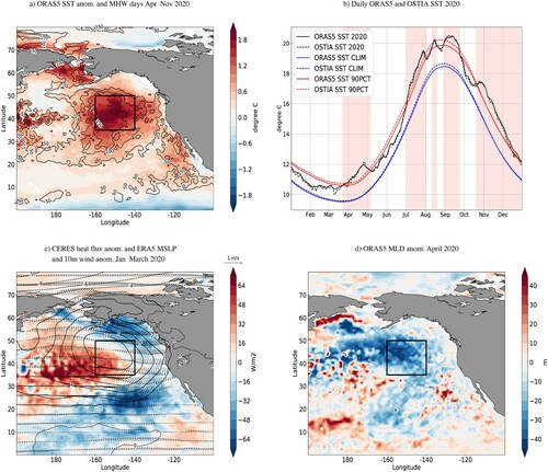
4.3.2.2. ORAS5 ocean reanalysis

This work investigates the characteristics of MHW events occurring in the North East Pacific in the ORAS5 reanalysis (Zuo et al. [Citation2019]; part of the product ref 1.3.1). ORAS5 is based on the NEMO3.4 physical ocean model (Madec Citation2008) run at a ¼ degree horizontal resolution with 75 vertical levels with level spacing increasing from 1 m at the surface to 200 m in the deep ocean. ORAS5 atmospheric boundary conditions are taken from ERA-Interim forcing until end of 2017, ERA5 until end of 2019 and ECMWF operations for the year 2020. The reanalysis is conducted with NEMOVAR (Weaver et al. Citation2005; Mogensen et al. Citation2012) in its 3D-Var FGAT (first guess at appropriate time) configuration. NEMOVAR is used to assimilate subsurface temperature and salinity, sea-ice concentration and sea-level anomalies (SLAs). SST is assimilated in ORAS5 by modifying the surface non-solar total heat flux based on the difference between modelled and observation-based SST analyses from HadISST2 (Titchner and Rayner Citation2014) until 2008 and the Near-Real Time OSTIA operational product (product ref 1.3.3) until end of 2020.

In ORAS5, the MHW events are detected from the SST field provided by the ocean potential temperature at the first model level (0.5 m depth). Subsurface temperatures and the depth of the mixed layer (defined as a density threshold of $0.01 kg m^{- 3}$ from the surface) from ORAS5 are also used for a deeper understanding of the MHW in the North East Pacific.

4.3.2.3. Seasonal forecast of marine heatwaves

ECMWF seasonal forecast system 5 (SEAS5; Jonhson et al. [Citation2019]) is used to assess the skill in predicting the North East Pacific MHWs in 2020 with respect to ORAS5. SEAS5 is based on an atmosphere-ocean coupled model. The atmospheric component is the ECMWF Integrated Forecast System (IFS). The ocean model component is the same as for ORAS5. Ocean initial conditions for hindcasts over the 1993–2020 period are taken from ORAS5. SEAS5 produces a 50-member ensemble of 7-month forecasts initialised every 1st of the month. Forecasts are based on the ECMWF Earth system model that couples the atmosphere, land, waves and the ocean. SEAS5 is a state-of-the-art seasonal forecast system, with a particular strength in ENSO prediction. Biases in extratropical jets and limited representation of teleconnections (Johnson et al. Citation2019) means we need to interpret seasonal predictions in the Extratropics with care. Even though SEAS5 cannot predict the exact observed weather features, it can provide indications on weather statistics on a monthly to seasonal basis. Seasonal forecast of ocean variables other than SST has so far received little attention, but recent work hints that SEAS5 forecast skill for the ocean heat content in the upper 300 m is comparable to the skill for SST in the Tropics, and even exceeds it in the Extratropics (McAdam et al. Citation2022).

Here we explore if SEAS5 can predict the occurrence of MHW events in the Northeast Pacific, their duration and amplitude over the forecast range 1–4 months. Forecasts starting on 1 February, 1 May and 1 August 2020 are used to assess the ability of SEAS5 to predict both the onset and the recurrence of the 2020 MHW events in spring (MAM), summer (JJA) and autumn (SON). The first 25 members of each forecast date are used for this assessment. Daily timeseries of SST forecasts are passed through the same detection procedure as ORAS5 using both the forecast SST mean and 90th percentile over the 1993–2016 reference period (same as for ORAS5). The statistics of the forecasts are spatially averaged for each SEAS5 ensemble member in the NEP area in the same way as ORAS5. The ensemble mean and spread of those statistics are then computed. The ensemble spread is a measure of the difference between the members and is represented by the standard deviation with respect to the ensemble mean. The probability of forecasting a MHW event is estimated at each grid point of NEP as the percentage of ensembles where the SST exceeds the 90th percentile for more than 5 consecutive days at any time during the considered season. The probabilities are then spatially averaged over NEP.

4.3.2.4. Additional datasets

Additional datasets are used not only for validation of the MHWs detected in ORAS5 but also to gain insight into the forcings influencing the occurrence of such event. ORAS5 SST is verified against the reprocessed (Good et al. [Citation2020]; product ref 1.3.2) and near-real-time (Donlon et al. [Citation2012], product ref 1.3.3) OSTIA 1/20° SST analysis based on both satellite and in-situ observations. ORAS5 subsurface temperatures are evaluated against the JMA 1°x1° ocean temperature analysis (Ishii et al., [Citation2017]; product ref 1.3.7) that is computed from subsurface ocean observations. Both the 10-m winds and the mean sea level pressure from the ERA5 reanalysis (Hersbach et al. [Citation2020], product ref 1.3.6) are used to explore the atmospheric forcings behind the occurrence of MHW events. MHWs are also influenced by heat fluxes at the air–sea interface. An independent estimate of the net surface heat flux is inferred from CERES-EBAF net TOA radiation (Loeb et al. [Citation2018], product ref 1.3.5) and the divergence of atmospheric transports computed using ERA5 data (Mayer et al. Citation2017; Mayer et al. Citation2021], which is deemed more reliable than parameterised fluxes taken directly from the reanalyses (see, e.g. Trenberth and Fasullo Citation2017).

4.3.3. Results

The 2020 MHW events in the Northeast Pacific are investigated in ORAS5 SST fields using 1993–2016 as reference period. Over the period April–November 2020, a positive mean SST anomaly larger than 2°C is detected off the North American coast and is centred in the NEP box (140–160°W/35–50°N, (a)) defined in the Products and Methods section. The timeseries of ORAS5 SST ((b)) in NEP shows strong agreement with the OSTIA SST analysis (product ref 1.3.2). Both the SST mean and 90th percentile over the 1993–2016 period from OSTIA are however slightly warmer than in ORAS5, meaning that ORAS5 will detect longer and more intense MHW events than OSTIA would. Such difference is probably linked to ORAS5 being constrained by a combination of HadISST2 (Titchner and Rayner Citation2014) until 2008 and then the Near-Real Time OSTIA operational product (product ref 1.3.3). This highlights the sensitivity of the MHW detection method from Hobday et al. (Citation2016) to the reference period used to compute anomalies. From spring 2020 onwards, ORAS5 SSTs reveal 5 MHW events in NEP ((b)). The first event started in April and lasted more than a month. It was followed by three shorter events in July, August and September and a longer one from October to Christmas. The first MHW detected in ORAS5 in April coincides with a long-lasting high-pressure anomaly from January to March centred over NEP, weak winds and a positive net heat flux anomaly into the ocean as seen in the inferred surface heat fluxes ((c)). These atmospheric conditions led to an anomalously shallow mixed layer in April ((d)). Seasonal MHW statistics presented in (a) (colour bars) indicate that NEP has seen on average 157 MHW days between March and November, 128 of which were classified as moderate event and 29 as strong event. There were nor severe neither extreme event. The most intense MHW happened during the summer (JJA) with a maximum amplitude of 3°C ((b)). Timeseries of seasonal MHW statistics in NEP ((d,e)) shows that 2020 is the year with highest number of days of MHW and the highest amplitude (in JJA 2020) of the past 10 years in the area.

Figure 4.3.2. (a) Average in NEP of the number of days of both moderate and strong 2020 MHW events during the MAM, JJA and SON seasons in both ORAS5 reanalysis (bars) and SEAS5 forecast ensemble mean (diamonds) and spread (error bars); (b) Same as (a) for the maximum amplitude (in degree C) of the 2020 MHW; (c) MHW seasonal forecast probabilities for MAM, JJA and SON 2020; (d,e) 2011–2020 timeseries of the total number of MHW days and the maximum amplitude (in degree C), respectively, of MHW events during the MAM, JJA and SON seasons for both ORAS5 and SEAS5 ensemble mean and spread. Both the spatial averaging over the NEP grid points and the computation of the ensemble mean can lead to numbers of MHW days below 1 day as grid points and/or ensembles that do not show any MHW are taken into account. In some cases, the ensemble spread can be larger than the ensemble mean (for example in 2018, where the distribution is skewed toward large values) and thus include negative values of number of MHW days.

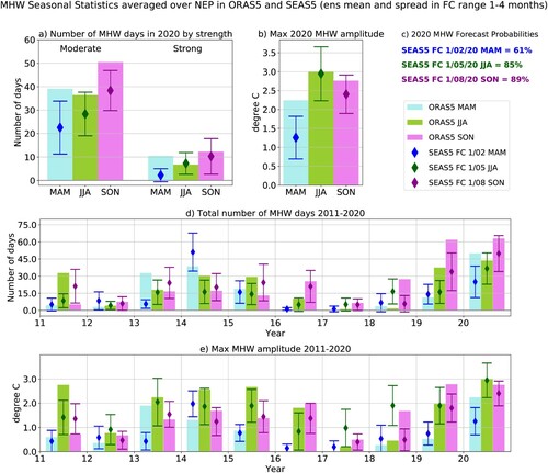
The 2020 MHW events in NEP are detected on the ocean surface following the Hobday et al. (Citation2016, Citation2018a) definition. But their occurrence strongly depends on both air–sea interactions and the long-term evolution of the upper ocean column. The 10-year timeseries of ORAS5 ocean subsurface temperature anomalies (with respect to the 1993–2016 mean) averaged over NEP in the layer 0–200 m (an approximation of the depth range of the euphotic zone) shows that the strong positive SST anomalies seen in 2020 are part of a warming signal that started in 2018 and now extends down to 150–200 m ((a)). The timeseries also captures the strong temperature anomaly of ‘the Blob’ that appeared in 2013 and ceased in 2016. Note that the NEP box only sees part of ‘the Blob’ as its maximum intensity was centred closer to the North American coast. In (b), timeseries of ocean temperatures averaged over the euphotic zone from both ORAS5 and the JMA dataset (Ishii et al. Citation2017) agree to show that the warming of ‘the Blob’ happened abruptly between 2013 and 2014, while the temperature increase from 2018 is more progressive, reaching averaged 2020 temperature anomalies of 1°C and 0.8°C, respectively, warmer than what is seen on average over 2013–2015 (around 0.54°C and 0.53°C, respectively).

Figure 4.3.3. (a) Depth-time plot of the ORAS5 (product ref 1.3.1) monthly potential temperature anomalies in NEP (colour-shaded) for the period 2011–2020. The solid grey line is the timeseries of ORAS5 monthly mixed-layer depth (MLD, in m); (b) monthly anomalies of potential temperature averaged in the layer 0–200 m (in degree C) for both ORAS5 (black) and the JMA dataset (red); (c) monthly anomalies of ORAS5 MLD (in m, blue) and Brunt-Vaisala frequency at 120 m (in s-1, green); (d) monthly anomalies of ERA5 10-m wind speed (in m/s, black) and mean sea level pressure (in hPa, blue) and of the net flux (in W/m²) from CERES-EBAF. The periods shaded in light red and blue correspond with the triggering and the end, respectively, of the MHW events discussed in the main text. All anomalies are computed with respect to 1993–2016 reference period.

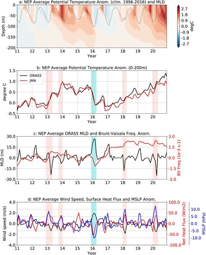
Timeseries of anomalies averaged over NEP of mean sea level pressure and wind speed from ERA5 and inferred net surface heat fluxes are shown in (d). They are analyzed in parallel with timeseries of ocean mixed layer depth and Brunt-Vasaila Frequency at 120 m (used as an indicator for the intensity of the stratification), both from ORAS5 ((c)). These timeseries indicate that, in NEP, anomalous events of high mean sea level pressure, low wind speed and high surface heat flux, as seen in winter 2020 ((c)), are coinciding with anomalously shallow mixed layers in ORAS5. This combination of signals is a common feature to the triggering of the ‘Blob’ in 2013 and its reemergence in 2018 (Gasparin et al. [Citation2020], (c)). Note that, in the NEP area, traces of ‘The Blob’ vanished in winter 2016 under the combined influence of low pressures, strong winds and anomalous heat loss leading to strong ocean mixing and deep ocean mixed layer (Peterson et al. Citation2016). Another interesting feature during this 10-year period is the sharp increase of the stratification at the base of the mixed layer seen since 2017 that reaches much higher levels than seen during the 2013–2015 period of the ‘Blob’ ((c)). Observations show that oceanic stratification increases with the warming climate (e.g. Li et al. Citation2020), and high stratification preconditions the upper ocean for recurring MHW events in summer and autumn as seen since 2018 in NEP NOAA ecosystem assessment reports (Ferriss and Zador Citation2021; Harvey et al. Citation2021) showed that the 2020 MHW is the second largest on record in the North Pacific. These reports use the information of the monitoring of MHW as one of the many aspects explaining the state of the ecosystems in 2020. Extended range forecasts are also used to give an outlook on the coming months and inform management authorities and marine industries. Skilful seasonal forecasts of MHW events would therefore be very valuable information for these stakeholders. Here we use ECMWF SEAS5 for a first assessment of the skill of seasonal forecast of the North East Pacific MHWs in 2020 following the procedure described in Products and methods. The statistics of the ensemble of forecasts are presented in (diamonds and error bars) for the forecast range 1–4 months. The forecast starting on 1 February 2020 can predict MHWs in the subsequent season (MAM) with a probability of 61%. Not surprisingly though, the ensemble mean underestimates the number of days of both moderate and strong MHW events but also the maximum amplitude of these events in MAM 2020 ((a,b)). The SEAS5 ensemble spread also does not capture the number of MHW days and the maximum amplitude seen in ORAS5. Forecasts starting in May and August 2020 both show probabilities of MHW events over 80% with number of days and amplitudes closer to ORAS5, in particular for JJA 2020 ((a,b,c)). Forecast uncertainties however remain high as shown by the ensemble spread.

These statistics suggest that it is easier for SEAS5 to predict the recurrence of MHWs during the summer and autumn 2020 than their onset in spring. One possible interpretation is that the MHW act as a cascade event, with the occurrence of the first one setting favourable conditions for recurrence. Hindcasts over the past 10 years show a mixed level of skill in predicting both the number of days and amplitude of MHWs ((d,e)). SEAS5 for example wrongly predicts around 15 days of MHW with a maximum amplitude around 2°C in summer 2018. Similarly, the start of ‘the Blob’ in spring 2013 looks poorly forecasted with small number of MHW days and low amplitude. The SEAS5 forecast suggests that the MHWs detected in 2020 were among the most predictable, probably because the ocean-atmosphere system was well preconditioned for these events to happen. Indeed, at the start of 2020, the upper ocean was already anomalously warm and stratified and the high atmospheric pressure system over the Pacific North East was well installed. However, both MHW forecasts and hindcasts need to be repeated in the future to put these results into context. The skill for longer forecast ranges should also be assessed as advance warning of MHW would be very useful.

4.3.4. Conclusions

Most literature on MHW detection and monitoring is based on observation-based daily SST analysis datasets (Oliver et al. Citation2020). From the example of the 2020 MHWs in the North East Pacific, ORAS5 shows there is potential for accurate near-real-time monitoring of MHWs from daily ocean reanalysis fields. The additional value of reanalysis datasets is to provide access to both the response of the ocean subsurface and its role in the generation and persistence of MHWs. Information on the processes behind the MHWs is available through both ocean and atmospheric reanalysis datasets and could be quantified via a heat budget analysis (Holbrook et al. Citation2019).

Ocean reanalysis datasets are spanning a few decades, which put the most recent MHWs into a long-term context. The 2020 MHW events in the North East Pacific happened in the context of a recent trend toward more frequent and longer heatwaves (Oliver et al. Citation2018; Collins et al. Citation2019). Favourable atmospheric conditions such as high mean sea level pressure and weak winds impact the upper ocean stratification making the ocean mixed layer more responsive to anomalous surface heat fluxes. The increased stratification at the base of the mixed layer seen since 2017 coincides with the resurgence of MHWs from 2018 onwards after the ‘Blob’ vanished in 2016 (). Near-real-time ocean reanalysis datasets will provide a continuous monitoring of the various aspects of the evolution of such MHW events.

While the monitoring of MHWs is interesting from a climate perspective, the ability to predict future events could be of great value. The North East Pacific is indeed a major fishing area where MHWs are known to impact ecosystems, migratory routes, and fish habitats. Information on the length and the strength of MHWs in the area can potentially influence the decision making of marine management authorities in terms of limiting the fishing of species vulnerable to such events for example. The ECMWF SEAS5 system showed skill in predicting the number days and amplitude of the 2020 events at seasonal timescales, albeit with large uncertainties as seasonal predictions in the Extra-Tropics in SEAS5 remain a challenge mainly because of model biases and limited representation of teleconnections (Johnson et al. Citation2019).

Seasonal forecast of MHW is already being explored in the Indo-Pacific region and the Australian waters (Hobday et al. Citation2016, Citation2018b). The work presented here only showed first order evaluation of a seasonal forecast of MHW with respect to an ocean reanalysis product. The aim was to show the potential for seasonal forecasting of MHW. More sophisticated diagnostics such as Relative Operating Characteristics (ROC) score (Kharin and Zwiers Citation2003) or reliability diagrams (Johnson et al. Citation2019) could be adapted to MHW forecasting in the future. But, before getting there, a significant amount of work is still required to construct skilful MHW metrics and products that are useful for stakeholders. Only then, a more complete evaluation package can be developed and routine production and verification of MHW predictions over areas of interest implemented in global and regional seasonal forecasting systems. Such forecast products could eventually be delivered to users from marine management and industries and help decision-making.

Funding

This study was partially funded by the European Union's Horizon 2020 Research and Innovation Framework Programme under grant agreement No 862626.

Section 4.4. Record high heat content and low ice extent in the Baltic Sea during winter 2019/20

Authors: Urmas Raudsepp, Ilja Maljutenko, Jari Haapala, Aarne Männik, Svetlana Verjovkina, Rivo Uiboupin, Karina von Schuckmann, Michael Mayer

Statement of main outcome: In winter 2019/20 (December to February), ocean heat content (OHC) anomaly (relative to the reference period of 1993–2014) in the upper 50 m layer of the Baltic Sea of 211 MJ/m² was the highest over the period 1993–2020. The climatological (1993–2014) winter (December to February) air–sea heat loss amounts to about 0.5 GJ/m² (64 W/m²) over the Baltic Sea. In winter 2019/20, air–sea heat flux anomaly was positive, 226 MJ/m² (29 W/m²), thus almost balancing positive OHC anomaly. In colder winters, ice formation could play a significant role in the air–sea-ice heat budget, with a climatological mean (1993–2014) latent heat of freezing of 18 MJ/m². Maximum ice extent in the Baltic Sea, which has been the main indicator of the severity of ice winters in the Baltic Sea, was the lowest (38,300 km²) on record since 1720 in winter 2019/20. In winter 2019/20, the small sea ice volume resulted in the anomaly of latent heat of ice formation of −15 MJ/m² (relative to climatological mean of 18 MJ/m²). Either the anomaly of OHC or anomaly of sea ice extent – the correlation coefficient between the upper 50 m layer OHC anomaly and maximum sea ice extent anomaly in December–February was −0.7 – can be regarded as a descriptor of the winter conditions in the Baltic Sea.

Products used:

Table

4.4.1. Introduction

The winter of 2019/20 was characterised by unusually warm conditions across northern hemisphere midlatitudes (Lee et al. Citation2020). The reason behind this warm weather was the extremely strong, i.e. cold and stable, stratospheric polar vortex during the northern hemisphere winter of 2019/20 (Lawrence et al. Citation2020). The strong stratospheric polar vortex was closely linked to a positive Arctic Oscillation (AO) pattern that influenced the regional distributions of temperatures and precipitation during late winter and early spring. High temperature and precipitation values were recorded over northern Eurasia, eastern Asia, and south-eastern North America in winter 2019/20 (Juzbašić et al. Citation2021). The Siberian heat wave (Overland and Wang Citation2021) and a remarkably low Arctic sea ice extent in 2020 (Lien et al. Citation2022) were the most prominent manifestations of this large-scale atmospheric circulation.

Positive temperature anomalies extended to north-eastern Europe in January and February 2020 (Overland and Wang Citation2021), thus covering the Baltic Sea region. An unusually high winter air temperature was measured in Poland (Tomczyk et al. Citation2021). Unusually warm weather in the 2019/20 winter is expected to have had an impact on ocean warming, as estimated through ocean heat content (OHC, von Schuckmann et al. Citation2020) and annual maximum sea ice extent of the Baltic Sea. Interannual variability in sea ice conditions and sea surface temperature in the Baltic Sea is driven by the large-scale atmospheric circulation characterised by the North Atlantic Oscillation (NAO, BACCII Author Team Citation2015 and the references therein). Annual Maximum sea Ice extent in the Baltic Sea (MIB) is controlled by the air temperature and OHC of the surface layer (Uotila et al. Citation2015).

Anomalous high OHC during winter could result in an earlier start of the spring phytoplankton bloom (Trombetta et al. Citation2019). Moreover, higher temperature in the water column in winter could accelerate oxygen consumption during organic matter oxidation and result in the worsening of oxygen conditions during the following summer and autumn (Thamdrup and Fleischer Citation1998; Brewer and Peltzer Citation2016). The sea ice is a required habitat for the pupping of ringed seals, and a limited sea ice extent directly affects their population in the Baltic Sea (Meier et al. Citation2004).

Surface layer temperature and sea ice respond rapidly to the changes in atmospheric heat fluxes. The sea ice conditions between consecutive ice seasons are independent because the thermal memory of the Baltic Sea is only 2–3 months (BACCII Author Team Citation2015). In this study, we will focus on the OHC of the upper 50 m thick layer of the Baltic Sea as well as sea ice extent (SIE) and sea ice volume (SIV) during the winter 2019/2020 months of December, January and February (DJF hereinafter). This integration depth was selected because a 50 m depth is close to the average depth of the Baltic Sea (Jakobsson et al. Citation2019) and also the local minimum of the OHC profile (Liblik and Lips Citation2019). This layer of the Baltic Sea has a positive temperature trend of about 0.05–0.06°C/year (lower bound of 95% confidence level is 0.04 and upper bound is 0.07°C/year) calculated over the 1993–2019 period (von Schuckmann et al. Citation2019). We use the DJF season for the definition of winter in order to be consistent with previous work about the Baltic Sea winters (e.g. BACCII Author Team Citation2015). In addition, we analyse surface energy balance and atmospheric heat fluxes over the Baltic Sea in relation to the OHC and SIE in winter 2019/20.

4.4.2. Data and methods

4.4.2.1. Calculation of the OHC

The daily ocean heat content, OHC, has been computed from reanalysis (product reference 4.4.1) and near-real-time model data (product reference 4.4.2) for each model grid cell using the methodology according to Meyssignac et al. (Citation2019), (1) $OHC = \int_{- 50}^{0} c_{p} ρ T Δ z$ (1) where ρ is the density of seawater calculated following the TEOS10 (IOC et al. Citation2010), c_p is specific heat capacity calculated as a third order polynomial function of salinity and temperature according to Millero et al. (Citation1973), Δz is layer thickness of the grid cell and T is daily temperature. Balmaseda et al. (Citation2015), Palmer et al. (Citation2017) and von Schuckmann et al. (Citation2018) have calculated OHC from different ocean reanalysis products.

The OHC (1) was integrated over the upper 50 m thick layer. The 50 m depth corresponds to the depth where water temperature in the central Baltic Proper in winter 2019/20 was higher than the climatological winter mean temperature for the period 1993/94–2014/15. Physically, the 50 m depth corresponds to the upper boundary of the permanent halocline in the Baltic Sea, which acts as the effective barrier for the seasonal vertical mixing of the heat. The OHC of the Baltic Sea was calculated for the domain of 53.0–65.9°N and 9.0–30.2°E. The OHC anomaly has been calculated relative to the mean winter (DJF) OHC of the reference period of 1993/94–2014/15.

4.4.2.2. The Baltic Sea model data

The Baltic Sea OHC is estimated using the BALMFC CMEMS reanalysis (product reference 4.4.1) from the period 1993–2019 and the near-real-time model (product reference 4.4.2) for the period 2019–2020. Two products have been used because neither of them covers the whole study period of 1993–2020. The reanalysis is based on the NEMO-Nordic model (Pemberton et al. Citation2017; Hordoir et al. Citation2019) where in situ profiles of salinity and temperature from the ICES database (www.ices.dk) and the sea surface temperature observations from OSISAF (http://www.osi-saf.org/) have been assimilated using the Localised Singular Evolutive Interpolated Kalman (LSEIK, Nerger et al. Citation2005) filter. The atmospheric forcing of the reanalysis (product reference 4.4.1) is from HIRLAM (High-Resolution Limited Area Model) with a 22 km resolution for the period 1993–2011 (Dahlgren et al. Citation2016; Landelius et al. Citation2016) and from the UERRA reanalysis product (European Regional analysis) with an 11 km resolution from 2012 onwards. Near-real-time model (product reference 4.4.2) results are based on the NEMO-Nordic 2.0 model (Kärnä et al. Citation2021). The satellite sea surface temperature level 3 product from SST_BAL_SST_L3S_NRT_OBSERVATIONS_010_032 has been assimilated to the model run using the PDAF assimilation method with a univariate mode. The atmospheric forcing of the near-real-time model (product reference 4.4.2) is from 2.5 km MetCoOP HARMONIE model forecast and ECMWF HRES forecast data in North Sea regions outside the MetCoOP domain. Two products, 4.4.1 and 4.4.2, with different grids have been resampled on a common grid for calculation of the OHC anomalies for the 2019/2020 winter compared to the reference period of 1993–2014.

4.4.2.3. Atmospheric fluxes

The Copernicus ERA5 climate reanalysis (product reference 4.4.5) was used to obtain heat fluxes with a ca 30 km horizontal resolution and hourly time resolution over the Baltic Sea region. The downward heat flux is positive while the upward heat flux is negative. Spatial maps of different air–sea surface energy budget components were calculated for the winter 2019/20. The DJF average net surface shortwave radiation (param 176) and net surface longwave radiation (param 177) at the surface were used together with sensible (param 146) and latent (param 147) heat fluxes. The fluxes were taken from monthly averaged single level fields. The net surface energy budget was calculated by summing all four fluxes. The reference values for all the components and surface energy budget of the DJF season were created using monthly averages over the 1993/94–2014/15 period. The spatially averaged values of the air–sea surface energy budget components for the Baltic Sea were computed using a domain similar to the one used for the OHC calculations.

4.4.2.4. Ice data and calculations

The satellite remote sensing data of ice coverage from the years of 1982–2020 is used. Copernicus product reference 4.4.3 provides daily sea ice concentration (SIC) data derived from the Swedish Meteorological and Hydrological Institute’s (SMHI) and the Finnish Meteorological Institute’s (FMI) high resolution ice charts at a 5 km horizontal resolution. The SIC is an estimated fraction of an area, which is covered by ice in the grid cell. A pixel is defined as ice-covered when the SIC of the pixel exceeds 0.15.

Daily SIE values are computed from the daily SIC maps as the sum of the area of the grid cells that have a SIC value larger than 15%. The product (product reference 4.4.3) provides SIE for the Baltic Sea from January 1993 until the present time.

Daily SIV values are computed from the daily SIC and sea ice thickness maps. The data used to produce the sea ice thickness maps are Synthetic Aperture Radar images as well as in situ observations from ice breakers. The SIV data may have larger uncertainties than SIC data because of the errors in the determination of the sea ice thickness (Raudsepp et al. Citation2019).

In order to provide a climatic perspective for recent sea ice changes, we also utilise MIB time series (Niskanen et al. Citation2009 and updates provided by the FMI).

4.4.2.5. Model validation

We have focused on the validation of the near-real-time model data to gain confidence about the estimates of the OHC in winter 2019/20. We have implemented the K-means clustering algorithm (Jain Citation2010) for the validation of the near-real-time model seawater temperature and salinity product (product reference 4.4.2) with FerryBox measurements (product reference 4.4.4). We use FerryBox temperature and salinity measurements from the winter months of the years 2018/19, 2019/20 and 2020/21. During the winter months of 2018/19, two ferries were operational. The first one operated between Helsinki and Travemuende. This line crosses the Baltic Sea from the Gulf of Finland to the southwestern Baltic Sea. The second ferry operated on the Helsinki–Tallinn route across the Gulf of Finland. During 2019/20 and 2020/21, only one ferry line between Helsinki and Travemuende was operational during those months.

The K-means model validation method is described by Raudsepp and Maljutenko (Citation2022). All available data that fall into the model domain and simulation period are incorporated into the skill assessment even if the verification data are distributed unevenly and/or occasionally sparse. The method enables to evaluate the model quality at each location and time instant where and when the measurements have been acquired. A two-dimensional error space (dS,dT), where dS = (S_mod-S_obs) and dT = (T_mod-T_obs), of simultaneously measured temperature and salinity values was formed as the basis for the clustering. We interpolated the model values from the model grid to the location of the measurements. In total, we had 325,821 simultaneous temperature and salinity error pairs for clustering. The K-means algorithm finds the location of the centroids of a predefined number of clusters in the error space. The location of the centroids represents the bias of the set of errors for each cluster.

The K-means clustering algorithm requires the number of clusters to be predefined. In order to find the number of clusters for final analysis, we run the K-means clustering algorithm for total number of clusters K = 1:9 with 100 iterations for the convergence of the locations of the clusters. The clustering was applied to the normalised errors. Normalization was done for temperature and salinity errors separately using corresponding standard deviations of the errors. Four error clusters were selected using the Elbow cluster selection criteria (Bholowalia and Kumar Citation2014; Yuan and Yang Citation2019) and by analysing the rationality of the distribution of errors in clusters (Hastie et al. Citation2009). The results of the K-means clustering for non-normalized errors are shown in (a), and the metrics are presented in .

Figure 4.4.1. (a) The Baltic Sea and its division into the different regions used in this study. The black dashed lines show the boundaries between the regions. The spatial distribution of the share of error points of the sum of data points belonging to the clusters k = 2 and k = 4 relative to the number of all data points at each grid cell (i,j) on the ferry routes along which the measurements were made. The colourbar shows the share of the sum of data points belonging to the clusters k = 2 and k = 4 to the sum of the all data points in the respective grid cell (i,j). The stars mark the start and end of the ferry routes (product ref. 4.4.2, 4.4.4). (b) The distribution of the error clusters for K = 4. The colourmap shows the logarithmic distribution of the number of salinity and temperature error pairs (model minus observation) in the 2-dimensional error space. Error bins have a resolution of 0.5°C for temperature and 0.5 g kg⁻¹ for salinity.

Table 4.4.1. The bias, root-mean-square error (RMSE), standard deviation (STD) and correlation coefficient (Corr) for each of four clusters (product ref. 4.4.2, 4.4.4).

In the formation of the error space, we retained the coordinates of each error point (dS,dT)(x,y), which enables us to map the errors belonging to each cluster back to the location where the measurements were performed. In order to do that, the model domain is divided into horizontal grid cells (i,j) of 1 × 1 km² size. Then the number of error points belonging to different clusters at each grid cell (i,j) is counted. Total number of error points belonging to the grid cell (i,j) is the sum of the points of each cluster. The share of error points in each grid cell belonging to cluster k is the ratio of the number of error points of cluster k and the total number of error points in each grid cell.

The salinity in k = 2 (bias of dS = 0.05 g/kg) and k = 4 (bias of dS = −0.11 g/kg) is close to observations, while temperature is marginally overestimated in k = 2 (bias of dT = 0.21°C) and underestimated in k = 4 (bias of dT = −0.42°C). These two clusters include the majority of datapoints, 126,711 and 180,031, respectively. Thus, we sum up the number of points belonging to the clusters k = 2 and k = 4 at each grid cell (i,j) and calculate the share of these points relative to the total number of points belonging to the respective grid cell (i,j). The points of these two clusters cover the entire trajectory of the ferry lines from the north of the Gulf of Finland across the Baltic Sea to the southwestern part of the Baltic, as their share is one ((b)).

The cluster k = 1 underestimates salinity (bias of dS = −2.2 g/kg, dT = −0.43°C) and cluster k = 3 overestimates salinity (bias of dS = 2.44 g/kg dT = 0.24°C), including 11,806 and 7273 data pairs, respectively. These points are located mainly in the south-western Baltic Sea with a very few of them in the Gulf of Finland. These points have reduced the share of the error points belonging to the sum of k = 2 and k = 4 to about 0.3 in the south-western Baltic Sea ((b)).

While the clustering provides explicitly the model bias relative to the data via the location of the centroids, common statistics like STD, RMSE and correlation coefficient can be calculated for the parameters belonging to each cluster. For instance, correlation coefficient, as well as STD and RMSE, is calculated between measured and simulated temperature and salinity values of each cluster separately (). The test shows that the model reproduces the temperature of the upper layer very well. The bias of model temperature and RMSE are in the range of −0.45–0.25°C and 0.4–0.7°C, respectively, as estimated for different clusters (). Therefore, we consider the data of a near-real-time model suitable for the estimation of the OHC in the upper 50 m layer.

General performance of NEMO-Nordic 2.0 model that is used for the near-real-time product without data assimilation is demonstrated by Kärnä et al. (Citation2021).

4.4.3. Results

The OHC anomaly in the upper 50 m thick layer in winter was calculated relative to the winter OHC of the reference period 1993–2014. On the background of a positive trend of winter OHC of 6.16 MJ/m² year⁻¹ (lower bound with 95% confidence level is 2.1 MJ/m² year⁻¹ and upper bound is 10.2 MJ/m² year⁻¹), winter 2019/20 stands out with an OHC anomaly of 211 MJ/m² (). The second highest OHC anomaly of 163 MJ/m² was in winter 2000/01. Significant interannual variability of the upper layer OHC is evidenced, as years with very high, moderate and very low OHC occur successively over the study period. For example, high OHC occurs in winter 2000/01, then returns to normal (climatological) conditions next year, followed by low OHC in 2002/03 ().

Figure 4.4.2. Time series of upper layer (0–50 m) ocean heat content (red), maximum ice extent (black) and maximum ice volume (blue) anomalies in the Baltic Sea in winter (December–February) (product ref. 4.4.1, 4.4.3, 4.4.6). The dashed line shows the trendline of upper layer ocean heat content anomaly over the period of 1993–2014 and the shaded area shows its 95% confidence level. The anomalies are calculated relative to the climatological winter (December–February) mean values. The climatological period is 1993–2014.

The maximum SIV and SIE anomaly calculated over the period of DJF compares well with the upper layer OHC (for SIV R = −0.80, 95% confidence limit: −0.90 … −0.60, p < 10⁻³) (for SIE R = −0.70, 95% confidence limit: −0.86 … −0.44, p < 10⁻³) (). There were cold winters in 2003 and 2011 with a high positive SIV anomaly and a negative OHC anomaly and a warm winter in 2020 with exceptionally high OHC anomaly and low SIV anomaly (). Such strong interdependence is not the case every winter. For instance, high OHC in 2001 and 2007 was not accompanied with exceptionally low SIV (). In 1994 and 1996, a high positive SIV anomaly of >30 km³ was present along with an only moderately negative OHC anomaly of about −100 MJ/m². We also note that from winter 2012/13 onwards the upper layer OHC anomaly of the Baltic Sea has been positive and the maximum SIV anomaly has been negative every winter ().

In winter 2019/20, the upper layer OHC was higher than the climatological mean over the entire Baltic Sea, including Kattegat and Skagerrak ((a) and (a)). The areas with the highest winter OHC anomaly were the Baltic Proper, western Gulf of Finland and the Gulf of Riga. In these regions, mean water temperature averaged over a 0–50 m depth and winter season (DJF) was between 4°C and 8°C ((b)). In the shallow coastal areas, the OHC anomaly was lower than in the open sea due to shallow depth of the area (smaller than 50 m integration depth) and differential cooling ((a,b)). The upper 50 m layer average temperature anomaly in the Baltic Sea in winter 2019/20 (December–February) was qualitatively similar to the OHC anomaly map. There is certain asymmetry of the OHC anomaly distribution between the western and eastern parts of the basins ((a)). In the Baltic Sea, mean water temperature of the upper 50 m layer is the highest in the southwestern part of the sea ((b)). A slightly lower but still high water temperature pattern extends to the east and then northward along the eastern part of the Baltic Sea ((b)). This temperature (and OHC) distribution pattern is consistent with general cyclonic circulation in the Baltic Sea (Meier Citation2007).

Figure 4.4.3. (a) Spatial distribution of upper layer (0–50 m) ocean heat content anomaly in the Baltic Sea in winter 2019/20 (December–February) (product ref. 4.4.2). The anomalies are calculated relative to the climatological (1993–2014) winter (December–February) mean spatial distribution (product ref. 4.4.1). The black contour corresponds to 211 MJ/m² ocean heat anomaly isoline. (b) The upper 50 m layer average temperature in the Baltic Sea in winter 2019/20 (December–February) (product ref. 4.4.2). (c) The number of ice days (sea ice concentration >0.15) anomaly in winter 2019/20 (December–February) (product ref. 4.4.3) compared to the climatological number of days during the ice season October–May. Black contours correspond to the climatological number of sea ice days.

Upper layer water temperature above 0°C prevented sea ice formation in the Baltic Sea, with the exception of the Bothnian Bay ((c)). Although sea ice has been present over a large part of the Bothnian Bay, the number of days with ice cover has been low, and only the coastal areas exhibit persistent ice coverage. The maximum number of 80–90 days with ice cover there is much lower than climatological ice duration (1982–2019) of 150–200 days in this part of the Baltic Sea (Raudsepp et al. Citation2020).

Climatological mean (1993–2014) winter (DJF) surface energy budget is negative over the entire Baltic Sea ((a)) with an average value of −93 W/m² (STD = 14 W/m²), which means that the sea loses heat during winter. Winter average (DJF) surface energy budget of the Baltic Sea in 2019/20 was also negative (not shown), but the energy budget anomaly relative to the climatological winter mean (1993–2014) was positive almost over the whole Baltic Sea ((b)). The spatial differences of the total surface energy budget anomaly ((b)) can be explained mainly by the spatial differences of the sensible heat flux anomaly ((e)) over the Baltic Sea. Regionally, the Bothnian Sea and central Baltic Proper had high surface energy budget anomalies of 42 and 32 W/m², respectively (). Main contributors to this regional pattern were positive anomalies of sensible ((f)) and latent heat fluxes ((e)). The low surface energy budget anomalies were in the Bothnian Bay (11 W/m²) in the far north and the Gulf of Finland (13 W/m²) in the east ((b), ). The surface shortwave radiation anomaly there was the highest, about 6 W/m², compared to the rest of the Baltic Sea ((c)). A sensible heat flux anomaly was also positive, about 11 W/m² ((f)). The negative anomalies of latent heat flux ((e)) and longwave radiation ((d)) compensated for positive anomalies of shortwave radiation and sensible heat flux.

Figure 4.4.4. Spatial distribution of winter (DJF) climatological mean (1993–2014) total surface energy budget (a), total surface energy anomaly in winter 2019/20 (b), shortwave radiation anomaly in winter 2019/20 (c), longwave radiation anomaly in winter 2019/20 (d), latent heat anomaly in winter 2019/20 (e) and sensible heat anomaly in winter 2019/20 (f) in the Baltic sea region. The heat fluxes are positive downward.

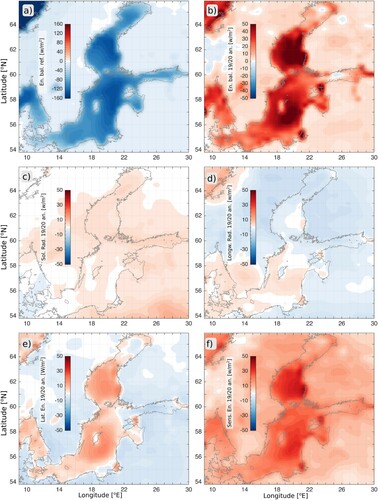
Table 4.4.2. Horizontal mean heat content anomaly (HC), surface energy balance anomaly (En) and corresponding heat (EnH) left in the sea over the three month period for the Baltic Sea subbasins in winter (DJF) 2019/20 (see ) (product ref. 4.4.1, 4.4.2).

Winter 2019/20 surface energy budget anomaly averaged over the entire Baltic Sea was 29 W/m², which would result in 226 MJ/m² of heat left in the upper layer of the sea compared to the climatological mean over the three-month period. Thus, the heat loss to the atmosphere was reduced by ∼30% compared to climatology, and the air–sea heat exchange anomaly (226 MJ/m²) explains the OHCanomaly (211 MJ/m²) in the upper layer of the Baltic Sea in winter 2019/20. Regionally, the comparison of the upper 50 m layer OHC anomaly ((a)) and the surface energy budget anomaly ((b)) of the Baltic Sea in winter 2019/20 shows a consistent pattern for the Baltic Proper and the Gulf of Riga. The OHC anomaly and the surface energy budget anomaly had high positive values over the Baltic Proper and the Gulf of Riga, nearly balancing each other (). As we are dealing with three-month average values, we cannot expect a perfect match of spatial distributions between the air–sea heat fluxes and OHC. The OHC anomaly was low, while the surface energy budget anomaly was relatively high in the Bothnian Bay (). In addition, the Bothnian Bay was partially ice-covered for at least a few weeks ((c)), which adds the latent heat of ice formation of 3 MJ/m². Climatological mean (1993–2014) latent heat of ice formation in the Baltic Sea is 18 MJ/m². The Bothnian Sea had the highest surface energy budget anomaly ((b)), but the OHC anomaly was moderate in comparison to the rest of the Baltic Sea ((a)) (). In the Gulf of Finland, the OHC anomaly was relatively high, while the surface energy budget anomaly was low (). Also, sea ice did not form in the Gulf of Finland in winter 2019/20 ((c)), which is consistent with relatively high OHC there.

The presence of warm and moist air over the Baltic Sea region inhibited sensible and latent fluxes from the sea to the atmosphere, which contributed to a high OHC. The potential effect of large-scale atmospheric circulation bringing warm and moist air into the region and inducing the anomalously high OHC of the Baltic Sea in winter 2019/20 is described by the winter mean NAO and AO indexes ((a,b)). The AO index was at its highest value over the period 1993–2020, while the NAO index was high but not the highest. The NAO had the highest value in winter 2015, when the previous record low MIB occurred (). Still, there are consistent variations of the NAO index, OHC anomaly and SIV anomaly starting from winter 2013/14. The NAO ((a)) and the OHC anomaly both have been positive while the SIV anomaly has been negative since then ().

Figure 4.4.5. (a) Time series of winter (December–February) mean NAO index. (b) Time series of winter mean (December–February) AO index. (c) Combined proxy-in-situ-airborne-satellite derived time series of the maximum annual ice extent of the Baltic Sea (left panel) and its distribution during 1991–2020 and the second mildest 30-year period in 1909–1938 (right panels).

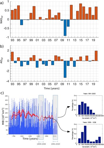
The MIB in winter 2019/20 was extremely low, 38,000 km² (product ref. 4.6.4), which is less than 10% of the Baltic Sea area. The long-term variability of the MIB shows that the winter period 1991–2020 has been the longest observed record of consecutive years with anomalously low MIB (∼30 years), whereas previous low MIB periods have been shorter (∼10 years) ((c)).

4.4.4. Discussion

The winter of 2019/20 was exceptional in terms of extremely high OHC anomaly in the upper 50 m layer of the Baltic Sea, with a small MIB and positive anomaly of the surface energy budget. In the long term context (winters 1993/94–2019/20), the OHC and sea ice conditions are strongly related. The correlation coefficient between the upper 50 m layer OHC anomaly and maximum SIE anomaly in DJF was −0.7 (−0.8 between SIV and OHC). Yet the spread around the linear fit was considerable for average and mild winters. In case of mild winters, i.e. 2007/08, 2014/15 and 2019/20, the maximum SIE anomalies were about −100,000 km², but the OHC anomalies were 84, 115 and 211 MJ/m², respectively (). Thus, the winter OHC of the upper layer of the sea and the MIB can be viewed as indicators of a winter marine heatwave.

Uotila et al. (Citation2015) analysed the extremely low MIB in winters 2007/08 and 2014/15 in relation to the local weather conditions and regional atmospheric conditions represented by the NAO index. They found a good correlation between the NAO and the MIB. There are numerous studies that relate mild winters with a positive NAO index (BACCII Author Team Citation2015 and the references therein). A positive NAO index means that strong westerlies bring warm air to the Baltic Sea region. In winter 2019/20, wind speed anomaly was up to 5 m/s and the air temperature anomaly was 3–6°C relative to the climatological winter period of 1993–2014 (not shown), which is consistent with strong westerlies. We have also established that high OHC in the upper layer of the Baltic Sea in winter 2019/20 can be explained by a positive anomaly of the surface energy budget in winter 2019/20. However, exceptionally warm conditions across Northern Hemisphere midlatitudes (Lee et al. Citation2020) in winter 2019/20 were closely linked to an exceptionally high positive AO index (Lawrence et al. Citation2020). On a global scale, the Baltic Sea region was located at the western rim of the warm air mass, which covered the Eurasian continent and adjacent part of the Arctic ocean (Overland and Wang Citation2021). The correlation coefficient between upper layer OHC anomaly and both the NAO and AO indexes were 0.5 calculated for the winters of 1993/94–2019/20. Between SIE (and SIV) and NAO (AO) the correlation coefficients were all −0.6. We suggest that extremely high OHC and low MIB are related to a simultaneous high positive NAO and an exceptionally high positive AO in winter 2019/20.

A winter warming has been detected in the Baltic Sea region (Kotta et al. Citation2018). In order to support that claim, we have shown that the winter OHC in the upper layer of the Baltic Sea increases with a rate of 6.12 MJ/m² per year. Recent studies have shown that not only does winter OHC increase, but also annual OHC has a positive trend in the Baltic Sea (Liblik and Lips Citation2019). Still, the OHC increase in the Baltic Sea is smaller than the global OHC trend (Holland et al. Citation2019; von Schuckmann et al. Citation2019) and in some other marginal seas (von Schuckmann et al. Citation2018; Lima et al. Citation2020). Trend values are low due to the shallowness of the Baltic Sea, which limits the accumulation of heat in the water. For instance, 86% of the Baltic Sea area is shallower than 100 m (Jakobsson et al. Citation2019). Therefore, the climate warming signal is more obvious in the water temperature than in the OHC. In the Baltic Sea, the water temperature trend of about 0.05°C/year at all depths has been estimated.

Although we have shown that there is good balance between the surface heat flux anomaly and the winter OHC anomaly in the upper layer of the sea, the regional differences between the subbasins of the Baltic Sea are still significant. The surface layer OHC anomaly of the Gulf of Bothnia was actually much lower than the part that can be explained by the surface energy budget anomaly (). The Gulf of Bothnia is deep and unstratified in winter (Haavisto et al. Citation2018), which points to intensive vertical heat exchange between upper and lower layers of the basin. The surface energy budget anomalies over the Gulf of Finland and the Bothnian Bay were comparable, 13 and 11 W/m², respectively, but the upper layer OHC was 29 times higher in the Gulf of Finland than in the Bothnian Bay (). There is extensive water exchange between the Gulf of Finland and the Baltic Proper (Liblik et al. Citation2018; Maljutenko and Raudsepp Citation2019), and the upper layer OHC in the Gulf of Finland was most likely significantly influenced by the heat transport from the Baltic Proper. Similarly, the OHC in the Gulf of Riga could be affected by heat transport from the Baltic Proper in winter (Raudsepp Citation2001), although in winter 2019/20 the net surface energy anomaly and the OHC were almost in balance (). The Baltic Proper, while being a source of heat for the Gulf of Finland and the Gulf of Riga, might receive warmer water from the Kattegat by the large volume inflows that mainly take place in winter (Raudsepp et al. Citation2018).

There are some shortages for which improvements are needed in order to fully understand the heat budget of the Baltic Sea. First, we would like to note that we used uncoupled models for the calculations of the atmospheric fluxes and the heat content of the Baltic Sea. The Baltic Sea heat content is estimated using the BALMFC CMEMS reanalysis (product reference 4.4.1) and near-real-time model data (product reference 4.4.2), while the ERA5 meteorological dataset (product reference 4.4.5) was used for the surface energy budget. Interactive coupling of the atmosphere and ocean models is particularly important during winter, allowing to obtain more adequate results in the distribution of the heat between atmosphere and ocean than non-coupled models (Gröger et al. Citation2015). Secondly, in this study we have not estimated heat transport between the subbasins of the Baltic Sea nor the vertical mixing of the heat between the upper 50 m thick layer and the water column below.

4.4.5. Conclusions

Under global warming, exacerbated weather and ocean conditions are expected (IPCC Citation2019, Citation2021). The current study represents the response of the Baltic Sea to the extremely warm weather conditions in winter 2019/20, which could be explained by the interaction of large-scale atmospheric circulations linked to a high positive North Atlantic Oscillation index and an unusually high positive Arctic Oscillation index. An unusually high heat content anomaly in the upper 50 m layer of the Baltic Sea in winter 2019/20 was detected. Heat content anomaly in the surface layer is negatively correlated with the maximum sea ice extent of the Baltic Sea and sea ice volume anomalies.

On average, the Baltic Sea energy loss to the atmosphere is approximately 93 W/m² during the winter season. Average energy loss to the atmosphere was smaller by 29 W/m² during the 2019/20 winter season due to a significantly warmer atmosphere and lower sea ice volume. This anomaly explained the excess heat storage of the topmost 50 m of the Baltic Sea. Exceptionally warm atmospheric conditions diminish the cooling rate of the Baltic Sea but do not reverse the overall winter cooling process.

Section 4.5. The September 2020 Medicane Ianos predicted by the Mediterranean Forecasting systems

Authors: E. Clementi, G. Korres, G. Cossarini, M. Ravdas, I. Federico, A. C. Goglio, S. Salon, A. Zacharioudaki, M. Pattanaro, G. Coppini

Statement of main outcome: From 17 to 20 September 2020, Medicane Ianos – a record Mediterranean tropical-like cyclone – hit the Ionian Sea and Greece with wind speeds up to 110 km/h, torrential rain and flooding, resulting in significant loss and damage in central Thessaly, particularly around the cities of Karditsa and Farsala.

The analysis of Medicane Ianos footprint in the Ionian Sea is provided by means of the numerical analysis data produced by the Mediterranean Monitoring and Forecasting Center (Med-MFC) and distributed within CMEMS. This analysis shows a significant change of the surface ocean fields such as an increase of currents, sea level, significant wave height, surface chlorophyll and a decrease of surface temperature during the event. The numerical solution has also demonstrated a change in the subsurface water dynamics with enhanced vertical velocity that affected mixing and the biogeochemical properties in the area during the medicane passage. The accuracy of the models is successfully demonstrated comparing with observations available in the area and during the period of interest. Moreover, we demonstrate that the quality of the numerical data is accurate enough to force a very high-resolution coastal model, which can provide improved representation (e.g. sea level peak) of such a severe event impacting the coastal areas.

Products used:

Table

4.5.1. Introduction

The Mediterranean Sea is one of the most cyclogenetic regions in the globe (Neu et al. Citation2013) and the cyclones generated in this region are known as medicanes or Mediterranean hurricanes (Emanuel Citation2005). These systems tropical-like cyclones and have been initially distinguished from other cyclones due to the formation of a characteristic cloudless ‘eye’ at the centre of a spiral cloud coverage (Fita et al. Citation2007; Tous et al. Citation2013). More recently medicanes have been suggested to correspond to cyclonic systems with symmetric, warm core structure (e.g. Cavicchia et al. Citation2014). Such warm cores have been shown to form due to the process of warm seclusion or due to the development of deep convection close to the cyclone’s centre, similar to tropical cyclones (Fita and Flaounas Citation2018; Miglietta and Rotunno Citation2019). Recent results show that the barotropic forcing is typically present in medicanes development, although strong convection is also expected to contribute significantly to the intensification of these systems (Flaounas et al. Citation2021). These low pressure systems, even if often originally of baroclinic nature, whenever they meet specific environmental conditions, can enter a new stage of development driven by convection and air–sea interaction rather than baroclinic instability, assuming features similar to those of tropical vortices, such as an almost perfect vertical symmetry, a spiral-shaped cloud cover with eye in the middle corresponding to a wind-less air column above the centre of the storm, and a warm core visible in the positive anomalies in the temperature field (Cavicchia et al. Citation2014).

Medicanes have typical size of the order of 300 Km in diameter, are more frequent during autumn and winter and can produce significant damage to socio-economic activities due to the combination of intense winds, heavy precipitation and enhanced ocean waves (Gaertner et al. Citation2018). Even though the frequency of medicanes is extremely low, 1.57 ± 1.30 events per year (Cavicchia et al. Citation2014), several authors (Romero and Emanuel Citation2013; Tous et al. Citation2016; González-Alemán et al. Citation2019) predict that medicanes will be less frequent in the future, but will develop a more robust hurricane-like structure and last longer, with higher winds and more rain. This means that the Mediterranean Sea region remains at high risk in terms of aggregate damages, given its large economy and long coastline. While cyclones have devastating effects when passing over coastal areas, over the ocean they can have a positive effect by enhancing productivity in oligotrophic areas (Lin et al. Citation2003; Menkes et al. Citation2016). The intensity of the ecosystem response to cyclones is the result of a trade-off between the depth at which cyclones mix the ocean and the depth of the nitracline and deep chlorophyll maximum (Menkes et al. Citation2016; Chai et al. Citation2021). While investigating the cyclone impacts by using satellite chlorophyll data may have some obvious limitations, 3D model outputs can provide insights on the coupling mechanisms (i.e. vertical transport of nutrients and phytoplankton growth) driving ecosystem productivity (Menkes et al. Citation2016).

Even though there is not an objective, commonly accepted definition of medicanes, the spiral cloud coverage and the development of a frontless, axisymmetric convective warm core characterising a Mediterranean cyclone impacting the Ionian Sea in September 2020, combined all the characteristics and processes that qualified this event as a medicane (Smart Citation2020) named Ianos. Medicane Ianos is considered to be one of the strongest such storms recorded since 1969 (i.e. since the beginning of satellite observations) in terms of duration and intensity, causing heavy rainfall, flooding, damages and death (Zekkos et al. Citation2020). This medicane formed off the Libyan coast over an area of low pressure in the Gulf of Sidra on 14th September and impacted the Ionian Sea and Greece from 17th to 20th of September 2020. In the following days, the Medicane intensified moving northward and eastward and reached its peak intensity on 18th September when it swept across Greece through central Thessaly, hitting mainly areas around the cities of Karditsa and Farsala. Medicane Ianos headed south towards the island of Crete while losing intensity in its south-eastward shift. Medicane Ianos brought high wind gusts reaching 110 km/h, torrential rain and flooding which caused the death of four people in Greece and huge damage to houses and streets (reported in Masters and Henson Citation2020; U.S. Department of Agriculture report Citation2020). An estimated 5000 properties were flooded in the city of Karditsa alone.

In the present study, we aim to investigate the ability of the Med-MFC analysis and forecast systems to represent Medicane Ianos and analyse its impacts on the physical, wave and biogeochemical upper layers fields.

4.5.2. Data and methods

The operational Near Real Time analysis fields produced by the CMEMS Mediterranean Monitoring and Forecasting Center (Med-MFC, products ref. 4.5.1, 4.5.2, 4.5.3) are used to analyse and assess their ability in representing Medicane Ianos evolution. The numerical products are derived from the integration of three operational systems that provide the main physical (MedFS, Clementi et al. Citation2021; product ref. 4.5.1), wave (Med-Wave, Korres et al. Citation2021; product ref. 4.5.2) and biogeochemical (Med-Bio, Salon et al. Citation2019; Feudale et al. Citation2021; product ref. 4.5.3) numerical fields. The three components are fully consistent (Coppini et al. Citation2021) and share the same bathymetry (GEBCO), same resolution, 1/24° in the horizontal and 141 vertical levels, and are forced by ECMWF (European Centre for Medium-range Weather Forecasts) analysis and forecast fields at 1/10° resolution (with 6-hours frequency for the analysis fields). The wave and biogeochemical systems are forced by MedFS physical fields. The three modelling systems are based on state of the art community models (NEMO: Madec Citation2016; WAM: WAMDI Group Citation1988; Komen et al. Citation1994; and BFM: Lazzari et al. Citation2012, Citation2016; Cossarini et al. Citation2015; Vichi et al. Citation2020), include the representation of tides and assimilate CMEMS observational in-situ data of temperature, salinity, chlorophyll, nutrients, as well as sea level anomaly, significant wave height and chlorophyll data inferred from ocean colour satellite measurements.

Model analyses are compared with available sea level observations derived from a tide gauge at the Katakolon station in the western Ilia along the Pelops coast of Greece (product ref. 4.5.5), CMEMS Sea Surface Temperature (SST) gridded satellite data (Buongiorno Nardelli et al. Citation2013) provided by the CMEMS SST-TAC (Thematic Assembly Center, product ref. 4.5.6) and along track satellite significant wave height provided by the CMEMS WAVE-TAC (product ref. 4.5.7) to highlight the strengths and shortcomings of the models and provide recommendations to further improve the forecasts and, possibly, reduce the damages caused by these events. Furthermore, using the biogeochemical numerical analysis product (product ref. 4.5.3), we verify the impact of Medicane Ianos on nutrients and phytoplankton vertical dynamics and ocean productivity. To track the medicane evolution, the wind intensity and direction derived from scatterometer and altimeter observations (provided by CMEMS Wind-TAC, product ref. 4.5.9), as well as the mean sea level pressure provided by ECMWF (product ref. 4.5.8) were analysed in the area affected by Medicane Ianos.

4.5.3. Results

Medicane Ianos began to grow on 14th September from a barometric low (around 1009 mbar) which developed in the Gulf of Sidra. Additionally, SST exceeded 27°C in this area and, together with the structure of the upper atmosphere, the barometric low began to acquire the characteristics of a tropical cyclone (Smart Citation2020). On 16th September the cyclone intensified and started moving north-northeast toward Italy. According to satellite data from scatterometer and altimeter observations, wind speeds exceeded 68 km/h in the central Ionian Sea and reached 76 km/h when passing near the southern coast of Italy (not shown). On 17th September the medicane, following the circulation of the upper atmosphere, began to move eastward with the maximum intensity of the winds above the sea, measured by satellite, reaching 88 km/h as its warm centre (at 995 mbar) was approaching the Ionian Islands. On 18th September Medicane Ianos’ centre entered the mainland of western Greece with wind speeds, as estimated by satellite, reaching (during morning hours) 71 km/h near the coast of Kefalonia. On 19th and 20th September Medicane Ianos moved southward, along the coasts of the western Peloponnese, and dissolved between Crete and North Africa. The decay of Medicane Ianos could be likely attributed to the most common tropical cyclones decay mechanisms such as the loss of energy from the sea moving inland and a change in the vertical wind shear (transitioning into an extratropical system).

Medicane Ianos evolution in the Ionian Sea was also tracked by means of low pressure centre locations (black lines in ) derived from the ECMWF 6-hours mean sea level pressure analysis fields from 16th to 18th of September, which confirm a northward direction in the first days, followed by an eastward pathway until September 18th when Medicane Ianos reached the Greek coastline.

Figure 4.5.1. Maps of surface fields from 16th to 18th of September (every 12 h): left panels: sea level (m); central panels: sea surface current (m/s) and direction; right panels: significant wave height (m) and direction. The path of the low pressure centres is also provided (black line), from 16th September at 12.00 (n. 1) to 18th September at 00.00 (n. 9) every 6 h. Products ref.: 4.5.1, 4.5.2 and 4.5.8.

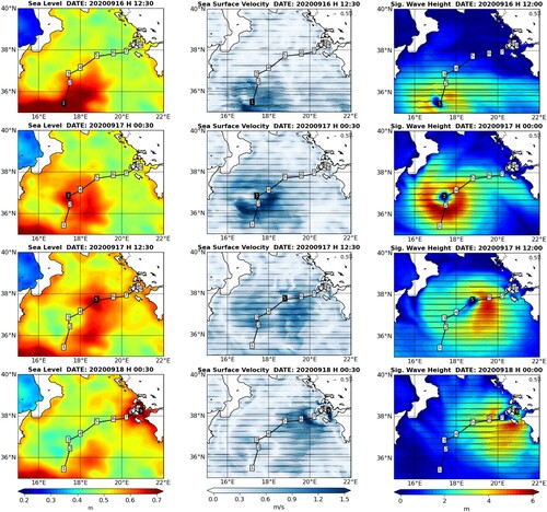
The impact of Medicane Ianos’ passage was clearly captured by hydrodynamic and wave models which simulated an increase of the sea level and significant wave height and an intensification of the surface currents along the medicane path as shown in . A strong signal occurred on 17th September at 00:00 UTC when the simulated sea level due to surge and tides reached 0.7 m, the surface currents increased up to 1.7 m/s and the significant wave height grew to 6.4 m. As the system moved eastward, 24 h later, Medicane Ianos hit the coasts of the Ionian islands causing huge damages on boats even in ports (Zekkos et al. 2019). At that time, the simulated wave heights reached a value of 5.9 m near Zakynthos with surface currents of around 1.8 m/s and sea level of 0.7 m.

The analysis of pre-storm conditions showed a continuous increase of the surface currents in front of Zakynthos until 18th September: specifically on 16th September at midnight the surface current velocity simulated by MedFS was 0.1 m/s, which increased to 0.4 and 1.8 m/s in the following 24 and 48 h respectively. To better examine the ocean response to Medicane Ianos in the Ionian Sea, several parameters have been calculated, based on the hydrodynamic model solutions and atmospheric forcing fields, following Price (Citation1983). Medicane Ianos was characterised by a quite large dimension with a radius to max stress (R) of 50 km, a stress magnitude of 0.64 N/m2 and a translation speed of 5 m/s with an inertial period of around 0.8 days. Thus, the non-dimensional storm speed (ratio of the Medicane residence time to the local inertial period) was around 0.5, which implies the surface mixed layer would be more dominated by the geostrophic currents rather than inertial motion (Price et al. Citation1991).

Numerical results were compared to measurements available in the area during the period of interest as shown in ; for the time series comparisons, the model grid cells closest to the observations were used. The model hourly mean sea level was compared to observations at the Katakolon Tide Gauge on the west Peloponnese coast showing general good agreement, with the model underestimation of about 4 cm from 17th September afternoon until the first hours of 18th September when the peak of the signal was registered. Since the reference levels of MedFS and tide gauge observations are different, a constant offset (81 cm) was added to the model values, corresponding to the mean difference between the modelled and the observed sea level in the considered period. The skill during the peak event is comparable to the mean sea surface height error (around 5 cm) which was evaluated by comparing model results with respect to more than 40 tide gauges in the whole Mediterranean Sea in a 3-year period (2017–2019). Furthermore, sea level results from a very high resolution (from 3 km in open sea to 100 m in coastal area) unstructured-grid system (based on the SHYFEM model, Umgiesser et al. Citation2004; Bellafiore and Umgiesser Citation2010; Federico et al. Citation2017; product ref. 4.5.4) initialised and nested into MedFS are provided for a coastal downscaling for the Zakynthos and Kefalonia areas (black rectangle in (b)). The main aim is to demonstrate that MedFS is accurate enough to provide both initial and boundary conditions to a very high resolution coastal model (the same approach adopted in Trotta et al. Citation2021). It is clearly evident that the downscaled model (HR-model in ) is augmenting the realism of the ocean hydrodynamics by adding geometry, resolution and specific coastal parametrisation, and can better capture the sea level peak in the first hours of 18th September with respect to the MedFS parent model during the event time. Moreover, in the considered period, the high-resolution model shows a slightly lower root mean square difference (HR-model RMSD = 2 cm) with respect to MedFS (RMSD = 2.4 cm) when compared to the Kataolon sea level observations (the statistics are evaluated after the offset removal).

Figure 4.5.2. Top-left panels: time series of sea level measured at Katakolon Tide Gauge (black line, Prod. Ref. 4.5.5), evaluated from the MedFS model (blue lines: solid line is the total SSH and the dashed line represents the surge contribution, Prod. Ref. 4.5.1), and from a High-Resolution unstructured model (red line, Prod. Ref. 4.5.4). Top-right panel: model topography, Katakolon Tide Gauge position (red circle), HR-model domain (black rectangle) and offshore (green) and coastal (yellow) areas impacted by Ianos Medicane. Central panels: SST (°C) anomaly between 19th September (after Ianos) and 14th (before Ianos) from model data (left, Prod. Ref. 4.5.1) and satellite (right, Prod. Ref. 4.5.6) including the Medicane Ianos path (black line). Bottom panels: comparison between modelled significant wave height (SWH, coloured area, Prod. Ref. 4.5.2) and satellite measurements (inset circles, Prod. Ref. 4.5.7) on 17th September, the inner figures depict the corresponding time series of measured (black) and modelled (blue) wave height along the satellite track.

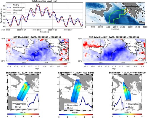
Between 14th and 18th of September, an SST decrease due to Medicane Ianos (around −3.5°C) was simulated by MedFS with some underestimation compared with the satellite L4 SST dataset (, central panels). However, we should consider that this observational dataset could not represent the small scale features present in the model solution due to the scarcity of direct observations along the Medicane track (caused by cloud covering), thus the SST L4 dataset is a combination of a first guess field with available data from previous days.

The evaluation of the wave model during the medicane was done using six satellite altimeters (Sentinel-3a/b, Jason3, Saral-Altika, CFOSAT and Hai Yang-2B) available through the CMEMS catalogue (product ref 4.5.7). (bottom panels) depicts examples of comparisons of the computed significant wave heights with measurements recorded along the tracks of satellites that crossed the area, providing maximum wave heights around 4.5 m. For this comparison, the model outputs were interpolated to the time of the observations. The results, summarised in , show that the accuracy of the modelled significant wave height is very good, and correlation between the observed and modelled data is high (ranges from 0.96–0.99) and the bias is close to zero varying from slightly positive to negative values.

Table 4.5.1. Significant wave height model skill on 17 September 2020 compared to Jason3, Saral and Sentinel 3B satellite tracks.

This good agreement between numerical data and observations suggests that the models correctly represented the sea level, SST and wave fields during the medicane.

To investigate the impact of Medicane Ianos on the ecosystem productivity, we compared the daily evolution of some physical and biogeochemical variables in the area affected by the medicane with the marine conditions outside its trajectory. We define here the impacted area as the area where the SST decrease on 20th September was at least 1.5°C with respect to the SST 1st–19th September time average and is divided into an off-shore (green area in ) and an in-shore (yellow area in ) domain. As a reference to evaluate Medicane Ianos impact, the unimpacted area in the Ionian Sea is delimited by LAT = 35°N–40°N and LON = 15.5°E–21°E where the SST change is less than 1.5°C. This subdivision was used to test the impact on open and coastal areas separately (following Menkes et al. Citation2016), and reflects two distinct moments in Medicane Ianos’ evolution: first, moving northeast in the open central Ionian Sea, then, after 18th September, approaching the Greek coast. The analysis shows no specific changes in the vertical eddy diffusivity ((a)), while, on 17th September, a peak in the upward vertical velocity ((b)) was reported (higher in the in-shore area), thus confirming the strong impact of the Medicane on the vertical structure of the water column along its passage. Based on that evidence we hypothesise that physical and biogeochemical properties of the water column within the impacted area were mostly affected by the upwelling associated with the wind stress curl. The isopycnal displacement of the thermocline due to storm-induced upwelling, computed as the ratio between the wind stress and the hurricane transit speed multiplied by the water density and Coriolis force (Price Citation1983), was estimated to be around 1.5 m (based on the characteristics of Medicane Ianos provided in previous paragraphs). Indeed, the nitracline depth uplifted approximately 10 m in correspondence with the vertical velocity maximum change ((d)) and the subsurface temperature (0–140 m) decreased 1°C in the area affected by Medicane Ianos ((c)). As a result of the enhanced vertical dynamics, nitrate concentration in the 0–140 m layer increased by about 10–15% compared to the concentration in the non-impacted area. A 20 m uplift of the deep chlorophyll maximum depth and an increase of about 20% of the chlorophyll concentration ((g–h)) occurred two-three days after Medicane Ianos’ passage. This generated the condition for the occurrence of a significant (with respect to the rest of the Ionian Sea, which is identified by the blue lines in (f)) increase of the productivity that lasted from the 22nd to 27th of September. Primary production increased by about 25–30% with respect to the conditions before the medicane event. Interestingly, during the medicane maximum intensity (17th–18th September), the productivity fell following a dilution of the biomass in the euphotic layer and a decrease of the light availability. Medicane Ianos caused more intense changes in temperature, nitrate and chlorophyll in the in-shore area than off-shore. However, the impact in the coastal area lasted for a short period which was not enough to drive a significant increase of productivity in the coastal area in the week after, and coastal conditions before the medicane event were eventually restored.

Figure 4.5.3. September–mid-October 2020 daily evolution of: vertical eddy diffusivity (a), vertical velocity (b), mean temperature in the layer 1–140 m (c), nitracline depth (d), mean nitrate in the layer 0–140 m (e), vertical integrated primary production (f), depth of the deep chlorophyll maximum (DCM; g), surface chlorophyll (h), mean chlorophyll in the layer 0–140 m. Each variable is evaluated in three different areas: off-shore impacted areas (green), in-shore impacted areas (yellow) and off-shore Ionian Sea not impacted by Ianos (blue). Lines and shadow areas are the median and the interquartile range; the vertical dashed red lines correspond to the initial and final dates of the event. Prod. ref. 4.5.1 and 4.5.3.

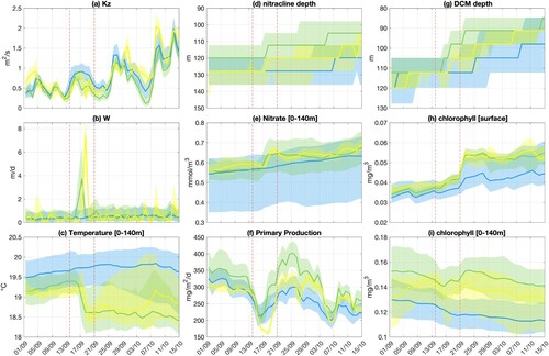
When comparing the biogeochemical impact of Medicane Ianos with those computed for tropical cyclones (Menkes et al. Citation2016), it emerges that the medicane was not strong enough to generate a complete and prolonged mixing of the water column. Indeed, given the strength of stratification and the depth of nitracline (> 120 m) before the medicane, the efficiency of the transport of nutrients in the euphotic layer by the medicane was limited (); and the injection of nutrients in the euphotic layer drove an increase of the system productivity that lasted for one week with a delay of 5 days in the open sea area. In the coastal area, the impact was more intense (higher drop surface temperature and higher increase of nutrient concentration) but very shortly dispersed and no significant impact on productivity was observed. Considering the trade-off between intensity of mixing and strength of stratification (Menkes et al. Citation2016) and the approaching autumn light limiting conditions, Medicane Ianos had mostly a local and short lasting impact on the ecosystem productivity of the Ionian Sea.

4.5.4. Conclusions and discussion

Medicanes are strong cyclones with subtropical and tropical characteristics that form in the Mediterranean Sea. Generating heavy precipitations and intense winds, they are consequently responsible for natural hazard along the Mediterranean coastal areas which are characterised by a high concentration of population. These catastrophic events as some authors have lately reported (Romero and Emanuel Citation2013; Walsh Citation2013; Tous et al. 2016; González-Alemán et al. Citation2019) will likely intensify over time due to their evident sensitivity to climate changes. Understanding the hydrodynamical, biogeochemical and wave conditions that take place during these extreme events is critical in order to mitigate the damage they can cause. In this context, accurate numerical modelling is an important and essential tool in the warning and forecast of these coastal hazards as well as to support risk and damage assessments and the design of coastal structures. In this study, we investigate how well Medicane Ianos (17–20 September 2020) is simulated by the Mediterranean CMEMS numerical systems.

The analysis of the impact of Medicane Ianos on ocean properties was undertaken using CMEMS Mediterranean analysis products and allowed a comprehensive assessment of its footprint on the Ionian Sea and Greek coastal areas affected by this event. Taking advantage from the alignment and the coupling between the physical, wave and biogeochemical components of the Mediterranean analysis and forecasting service, we show to which extent this medicane perturbed the surface ocean fields in terms of sea level, currents, temperature, wave height and chlorophyll, but also the vertical dynamics by increasing the mixing and consequently affecting the biogeochemical properties at depth.

Thanks to observations available in the period and area of interest, especially from satellite missions, the model solutions were validated showing a general good skill in representing the increased sea level, wave height and decreased temperature. The physical system has also proved to be accurate enough to force a downscaled high-resolution application, which in turn can provide improved representation of severe event impacts on the coastal areas.

Thus, this work shows that the oceanic fingerprint of cyclone Ianos was clearly and successfully captured by the Med-MFC analysis and forecast systems and that the produced data could also provide accurate boundaries to high resolution coastal applications. Considering the outcomes of this analysis, we emphasise the benefit in using CMEMS analysis and forecast data when extreme phenomena like medicanes occur and propagate over oceanic areas and eventually affect near coastal areas with potentially disastrous results.

Funding

The work has been supported by the Copernicus Marine Service funded by the European Commission (74-CMEMS-MFC-MED) and partially funded by the STREAM project (Interreg V A Italy-Croatia CBC Programme - Strategic Project ID: 10249186) funded by the European Commission.

Section 4.6. Extreme marine heatwave in the eastern Mediterranean in May 2020

Authors: Dimitra Denaxa, Gerasimos Korres, Maria Sotiropoulou, Leonidas Perivoliotis

Statement of main outcomes: In mid-May 2020, the eastern Mediterranean Sea experienced an unprecedented atmospheric heat wave which in turn generated a marine heat wave (MHW) event of remarkable intensity. The MHW affected almost the entire eastern basin, particularly at 18 May with maximum sea surface temperature (SST) anomalies exceeding 6°C and it was categorised as Extreme following the categorisation scheme proposed by Hobday et al. (Citation2018). Locations experiencing the most severe MHW conditions were identified particularly within the geographical area of 34°N–36°N. Τhe spatiotemporal evolution of the surface MHW conditions was associated with persistently weak winds and the consequent suppression of turbulent heat fluxes. A significant increase of the SST diurnal cycle was found in the southern Aegean, also attributable to the prevailing wind conditions during the MHW. Results suggest that the synergy of the concurrent extreme atmospheric heat wave with the prevailing weak winds (leading to the decrease of surface heat losses and mixed layer shoaling) have caused the observed extreme SST anomalies. Considering the increased occurrence of oceanic extremes in the basin and the associated severe impacts, this work aims to highlight the importance of reporting and studying such abrupt events, especially in ‘hotspots’ of climate change such as the Mediterranean Sea.

Products used:

Table

4.6.1. Introduction

The increasing need to better understand air–sea interaction processes and the ocean’s role within a warming climate renders the ocean’s temperature and in particular the SST a major climate change indicator. Studies on the effects of warming extremes in ecosystem functioning have highlighted the importance of exploring extreme events in addition to the analysis of long-term trends (Jentsch et al. Citation2007). In this context, research on oceanic extremes such as MHWs is rapidly growing.

According to the widely used definition of Hobday et al. (Citation2016), MHWs are discrete prolonged anomalously warm water events in the ocean. Recent studies have so far revealed that their frequency and duration have increased over the past four decades (Oliver et al. Citation2018; Holbrook et al. Citation2019; IPCC SROCC, Citation2019; Darmaraki et al. Citation2019a). Additionally, future projections at global and regional scales have shown that the intensity of MHWs will grow in the future (IPCC SROCC, Citation2019; Oliver et al. Citation2019; Hayashida et al. Citation2020). Research in this field is receiving focus over the recent years also due to a series of MHW events around the world associated with devastating ecological impacts (local extinctions, geographical shifts of marine species, impacts on primary productivity, coral bleaching, habitat loss, mass mortality events) as well as socioeconomic effects (fisheries, aquaculture) (Garrabou Citation2009; Wernberg et al. Citation2016; Frölicher and Laufkötter Citation2018; Smale et al. Citation2019).

Significant warming trends are computed for the last four decades based on L4 satellite SST observations for the entire Mediterranean Sea as well as for the western and eastern sub-basins (Pastor et al. Citation2020; Pisano et al. Citation2020). Future projections suggest additional warming (Adloff et al. Citation2015; Soto-Navarro et al. Citation2020) and increase of the occurrence of extreme SST values (Alexander et al. Citation2018) until the end of twenty-first century. Significant positive trends for the same period are reported for most MHW properties in the basin. Additionally, longer and more intense MHWs are predicted for the future, mostly attributed to the increase of the mean SST and to a certain extent to the daily SST variability (Darmaraki et al. Citation2019b). Studies of specific MHWs in the Mediterranean, such as the widely known summer MHW of 2003 (Sparnocchia et al. Citation2006; Olita et al. Citation2007), have significantly contributed to understanding the physical causes and implications of MHWs.

In mid-May 2020, Greece and the eastern Mediterranean basin experienced an unprecedented atmospheric heat wave. The extreme atmospheric event was caused by an early shift of the Jet Stream north of Greece that allowed for the transport of very warm air masses from Africa affecting the lower atmospheric layers over Greece and the eastern Mediterranean basin (Mavrakis et al. Citation2021). Under particularly weak winds, the aforementioned event generated the MHW discussed in the following.

4.6.2. Methodology

Three-hourly SST recordings from two fixed buoy stations north of Crete (named as 61277 and HERAKLION, included in product 4.6.1) have been used to gain insight into the warming event during May 2020. The buoys are located at 35.73°N – 25.13°E (61277) and 35.43°N – 25.08°E (HERAKLION), as depicted in (c). Both stations also record air temperature and wind at 3 m above the surface. Sea temperature recording depths of 61277 are: at 1, 20, 50, 75, 100, 250, 400, 600 and 1000 m while HERAKLION records at 1 m depth. The 1m-SST time series from the two stations present very similar behaviour during the period of interest. The buoy data analysis presented herein ((a)) is based on the 61277 buoy station which is located farther from the shore and provides temperature recordings at several depths.

Figure 4.6.1. (a) Temperature measurements from buoy (product 4.6.1) and satellite (product 4.6.3) data at the fixed 61277 platform location (35.73°N–25.13°E) during May 2020. Blue marks stand for daily mean buoy SSTs at 1 m and the associated bars define the corresponding diurnal range. Orange marks represent mean daily water temperature at 20 m from the same buoy. Green dots represent the satellite nighttime SST. Dashed purple line shows the mean daily wind speed evolution throughout the event. (b) Application of the Hobday et al. (Citation2016) methodology for the May 2020 MHW detection at the same location as in (a), using historical and NRT SST data from products 4.6.2 and 4.6.3, respectively (c) Temperature profiles from Argo float 6902847. Different colours (blue, red, purple) represent different time periods relative to the MHW evolution (before, during and after, respectively). The path followed by the float within the days considered in this graph extends from 34.83°N–22.71°E (May 6) to 34.43°N–22.95°E (May 26).

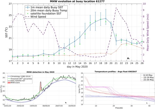
From the same CMEMS product, temperature profiles recorded in May 2020 from three Argo floats in the eastern Mediterranean were also examined (named as 6902847, 6902873 and 3901908). Profiles presented in this section are derived from float 6902847 which provides recordings at locations of high surface MHW intensity and at daily frequency (5-daily for the others) allowing for a better subsurface temperature monitoring. The path followed by the 6902847 float within the period where the temperature profiles were extracted extends from 34.83°N – 22.71°E (May 6) to 34.43°N – 22.95°E (May 26). The respective coordinates for 6902873 and 3901908 are 33.58°N – 24.70°E (May 5) to 33.26°N – 24.35°E (May 25) and 33.18°N – 28.54°E (May 6) to 33.44°N – 29.25°E (May 26), respectively.

MHW identification and analysis of relevant properties was performed in order to reveal the spatial extent of the warming event and assess its severity using common methodologies. The widely used MHW definition suggested by Hobday et al. (Citation2016) was applied on satellite foundation gridded SST data (products 4.6.2 and 4.6.3) for a selected domain covering the eastern Mediterranean Sea. According to this definition, the MHWs detected were discrete events lasting for at least five consecutive days, with temperatures warmer than the 90th percentile (as depicted in (b)). The latter was computed at each day from a 32-year historical baseline period. The climatological period used is 1982–2014. Additionally, an 11-day window centred at the day of computing the daily climatology was used, as well as a 30 day-window for smoothing the daily climatological threshold time series. For each grid point, we applied the categorisation scheme of the discrete MHW severity categories (Moderate, Strong, Severe, Extreme) presented in Hobday et al. as well as its slight variation by Sen Gupta et al. Citation2020 approach. According to the latter we used the following continuous Severity Index (SI) which additionally allows for ranking extreme MHW conditions: $S I_{i, j, t} = \frac{T_{i, j, t} - T_{i, j, d}^{c l i m}}{T_{i, j, d}^{90 t h} - T_{i, j, d}^{c l i m}}$ where $T_{i, j, t}$ is the SST of grid point at the i, j location of the domain at day t, $T_{i, j, d}^{c l i m}$ is the mean climatological SST for the same location in the climatological day-d corresponding to the actual day-t and $T_{i, j, d}^{90 t h}$ is the 90th percentile calculated for the specific location and climatological day.

Finally, CMEMS surface wind analysis observations (blended 6-hourly mean wind fields at 0.25°×0.25°; product 4.6.4) and turbulent heat fluxes (latent, sensible), wind speed and air temperature at 2 m above the surface from the ERA5 Reanalysis (daily mean values at 0.25°×0.25°; product 4.6.5) were used to investigate the conditions favouring the MHW evolution.

4.6.3. Results

4.6.3.1. Findings from in situ data

As presented in (a), SST at 1 m depth from station 61277 started to increase from 18°C at 9 May reaching a maximum daytime value of 26°C at 19 May. Satellite derived SST data from the high resolution near real time product 4.6.3 agree with the buoy observations at 1 m depth, although small differences occur among the two products with the daily averaged in situ SSTs being slightly higher. This is due to the fact that satellite observations are representative of foundation SST corresponding to nighttime values (00:00 UTC nominal time). Consequently, a larger daily mean temperature at 1 m depth compared to the nighttime satellite SST is expected. The slightly higher buoy-satellite SST differences appear during the first days of the surface warming. However, during the peak of the event this difference decreases and eventually the satellite SST slightly exceeds the buoy SST. This reversal appears probably because during the peak of the surface warming, 1 m is no longer a good proxy for SST at the surface. Under conditions of enhanced vertical stratification (favoured by the diminished winds, as discussed below) a larger temperature vertical gradient is expected very close to the surface, counterbalancing the daily mean – nighttime difference.

The SST evolution at the same location follows to a large extent the surface air temperature during May 2020 (not shown). Due to the poor availability of good quality 61277 air temperature recordings for the period of interest, the correlation of mean daily buoy SST with surface air temperature during the event is examined using the ERA5 air temperature at 2 m (closest value to buoy location). Pearson’s correlation coefficient reaches the value 0.94, while large correlation during the month is also found between the mean daily buoy SST and air temperature at 3 m as recorded by the HERAKLION buoy (not shown). As the surface warming progresses, also the SST diurnal cycle progressively increases ((a)), reaching up to 3.2°C at 17 May – a value 10 times larger than the diurnal cycle recorded before the event (9 May).

Eleven days after the initiation of the surface warming event (20 May) the temperature at 20 m-depth (T-20 m) does not present any noticeable increase. However, from that date onwards, an abrupt warming takes place at this depth, strongly linked with the change of the wind speed occurring at that time. In particular, by 23 May T-20 m increases by 2°C, due to the onset of wind-induced vertical mixing that transfers the surface warming signal to deeper layers, as discussed later in the Section. At 50 m-depth (as well as at the greater recording depths available at this location) the warming signal is not detectable (not shown).

Exceptionally low near surface wind speeds during the whole MHW were recorded by the same buoy at 3 m above sea surface ((a)). The initiation of the surface warming coincides with a decrease in the surface wind speed (9 May), while for the next 10 days the persistently low winds enhance the SST increase. From 19 May, the wind speed increases from 2 m/s to more than 9 m/s within 2 days, coinciding with the beginning of the decline of the surface warming event.

Before the MHW occurrence, surface waters are well mixed, given the almost equal T-1 m and T-20 m recorded values. During the surface MHW growth (that happens as long as winds remain weak), T-20 m remains unaffected by the surface warming indicating that near surface mixing is ceased and waters become more stratified in the vertical. It is only after the sharp increase of the wind speed that happens at 19 May that we observe a subsurface (20 m) temperature increase while SST starts to decrease due to vertical mixing switched on by the winds. As a consequence, the SST – T-20 m difference which was 6°C at the peak of the event gradually reaches values less than 1°C, indicating that wind induced vertical mixing transports heat deeper. Based on the above we assume that the recorded temperature increase at 20 m resulted from the vertical mixing that took place due to the winds abrupt increase from almost calm conditions.

The persistently low winds during the event also explain the large increase in the SST diurnal range reported above. Diurnal SST amplitude is generally expected to increase significantly under favourable conditions of intense solar insolation and weakened winds and can even exceed values of 5°C (Kawai and Wada Citation2007; Merchant et al. Citation2008). On the other hand, under normal wind-driven vertical mixing conditions in the oceanic upper layer and turbulent heat exchanges at the sea surface, the diurnal amplitude is expected to be much smaller. This is confirmed by the observed diurnal cycle before and after this MHW ((a)). In the case of high wind speed, the increased mixing can also completely cancel the effect of the high insolation and thus lead to an almost constant temperature in the upper metres of the ocean (Jansen et al. Citation2019). Indeed, this is consistent with the observed equal values of T-1 m and T-20 m during the first third of the month as well as with their convergence, as an immediate response to the increase of wind magnitude, during the last third of the month.

The temperature profiles from the three Argo floats show the evolution of the mixed layer warming and the progressive decrease of its thickness during the MHW (10–20 May, with small variations depending on the location). In specific, temperature profiles for 5 consecutive days before the beginning (6–10 May), during the peak (15–19 May) and during the decline (22–26 May) of the event are presented in (c) for float 6902847. The intense surface warming under the ceased winds ((c)) has caused the high stratification indicated by the sharp temperature gradient during the event as shown by the Argo profiles. During the MHW decline, heat penetrates through vertical mixing to the adjacent layers below the surface forming a mixed layer warmer by approximately 2.5°C with respect to the situation before the event. The observed vertical mixing after 20 May ((c)) takes place concurrently with the wind amplitude increase in the area ((c)). The other two sets of Argo temperature profiles (not shown) indicate the same wind effect on the water column during the event (mixed layer shoaling followed by wind-driven vertical mixing). The warming signal obtained by float 6902847 profiles is detected down to 30 m (same for the 6902873). The third set of profiles (float 3901908) measured further to the east shows that the warming signal penetrated to a depth of 50 m.

4.6.3.2. MHW identification in the eastern Mediterranean

Results from the MHW identification and categorisation methodology show that the area of buoy 61277 experienced an Extreme MHW ((b)). It lasted 10 days (13–22 May) peaking at 18 May with maximum SST anomaly (with respect to the local climatology for that day of the year) exceeding 6°C. This SST anomaly is found to be a local record-breaking event based on the satellite data for the period 1982–May 2020 used in this study.

At the same day (18 May) almost the whole domain experienced MHW conditions: at least Strong in more than half of the domain, and Severe up to Extreme conditions, shaping two particular ‘patches’, surrounding (northern and south-western of) Crete and south-eastern of Rhodes respectively ((c)). The maximum value of the SI for this day appears to the south-west of Crete. Although both aforementioned areas experienced Extreme MHW conditions during the month, it was for the location south-western of Crete at 18 May that the SI reached its maximum value. This area experienced the ‘most extreme’ MHW conditions during the whole event.

Figure 4.6.2. (a) Maximum MHW intensity (maximum SST anomaly with respect to local climatology for each calendar day) during May 2020; (b) Day in May 2020 when maximum MHW intensity occurred (c) Categorisation of MHW conditions at 18 May in the eastern Med using the continuous Severity Index (SI) following Gupta et al., 2020. SI ranges (1–2], (2,3], (3,4] and higher than 4 correspond to Moderate, Strong, Severe and Extreme MHW categories, respectively. Triangles mark the 61277 and HERAKLION buoys locations (offshore and coastal, respectively). In all panels, non-coloured sea grid points of the domain stand for no MHW conditions.

The spatiotemporal evolution of the most intense MHW conditions in the domain during May 2020 is examined based on the highest MHW intensity values in the month and the day when they occurred ((a) vs (b)). The spatial pattern of the maximum MHW intensity in (a) shows that the highest SST anomalies appeared particularly within the geographical area 34°N-36°N. Three clearly defined MHW centres of very high SST anomalies (with maximum values exceeding 6°C) during May 2020 are observed. The one located in the western part of the domain peaks at 18 May while the central and the eastern ones peak 2–3 days later ((b)), still linked to the same large-scale episode covering the whole eastern Mediterranean basin. These anomalies are found to correspond to the highest severity (Severe and Extreme) MHW categories. The two Argo floats south-west of Crete and the one in the central Levantine Sea captured temperature profiles in locations of Extreme/Severe and Strong surface MHW conditions, respectively.

Wind speed, air temperature and surface latent and sensible heat fluxes during the event are examined in order to explore the driving mechanisms of the large surface SST anomalies observed in the northern Levantine Sea. The Hovmöller diagrams presented in show the temporal evolution of the above parameters averaged in the latitudinal zone 33.5°N-37°N. Air temperature (ERA5 Reanalysis, product 4.6.5) and SST rise concurrently and the MHW centres discussed above present very high air temperature values at the respective MHW peak days (e.g. May 18 at 24°E, (a,b)). Further supporting the key-role of wind as it was observed by the buoy station in the Aegean, the L4 CMEMS surface wind product (4.6.4) confirms that the Strong/Extreme MHW conditions coincided with particularly low-wind conditions ((c)). The decline of the MHW appears as a response to the increase of the wind magnitude. ERA5 wind and SST data (not shown) are also examined for consistency with the use of ERA5 air temperature and heat fluxes and confirm the above findings.

Figure 4.6.3. Hovmöller diagram for CMEMS SST (a), ERA5 air temperature at 3 m (b), CMEMS wind speed (c) and ERA5 latent heat flux (d). For all parameters, diagrams depict daily mean values for the period 1–31 May 2020, averaged for the latitudinal zone 33.5°N–37°N.

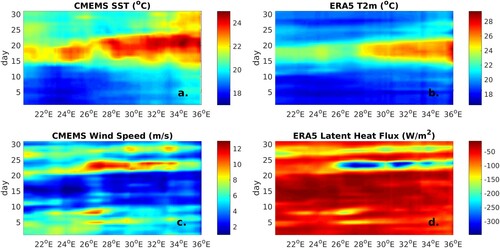
Air–sea heat fluxes occurring in the eastern Mediterranean Sea during May 2020 are indicative of the effect of the high air temperatures and the low wind conditions that prevailed over the area. During the evolution of the MHW a significant reduction of the latent heat loss took place ((d)) accompanied by an increase of the sensible heat gain (not shown). Both mechanisms enhanced the suppression of heat loss during the event. This situation is reversed as soon as the wind strengthens causing the observed drop in surface air temperature, the increase in sensible and particularly latent heat losses from the sea surface and the consequent MHW decline. Results suggest that the synergy of the concurrent extreme atmospheric heat wave with the prevailing weak winds (leading to both the decrease of surface heat losses and mixed layer shoaling) have caused such extreme SST anomalies.

4.6.4. Discussion and conclusions

The MHW that occurred in mid-May 2020 in the eastern Mediterranean Sea was formed following an extreme atmospheric heat wave and evolved as a MHW categorised as Extreme. The most intense MHW conditions are observed within the geographical area of 34°N–36°N. The magnitude and timings of the rise in SST as well as the spatial distribution of the highest MHW intensity were associated with the persistently low wind speed and the wind spatial distribution, respectively.

Under the specific atmospheric conditions and the highly stratified waters near the surface, the SST diurnal amplitude at the fixed platform 61277 located north of Crete (35.73°N–25.13°E) increased significantly, exceeding 3°C. The downward penetration of the surface warming as observed by the same station is detected at 20 m only after the mixing induced by the wind increase. Two Argo floats south-west of Crete and one in the central Levantine Sea captured temperature profiles in locations of Extreme/Severe and Strong surface MHW conditions respectively. The former two sets of profiles show that the warming signal reached approximately 30 m, while for the latter the corresponding depth is 50 m. The wind effect on the water column throughout the event (mixed layer shoaling followed by wind-driven mixing) is similar in all examined profiles.

Under the calm wind conditions during mid-May 2020 in the eastern Mediterranean Sea the air–sea heat fluxes and particularly the suppressed latent heat loss along with the intense stratification have been the major contributors for this MHW. They are common MHW favouring conditions (Holbrook et al. Citation2019; Sen Gupta et al. Citation2020) and they have also driven the extreme MHW of 2003 (Sparnocchia et al. Citation2006; Olita et al. Citation2007). Similarly to the May 2020 MHW, during a heatwave in June 2007 the Aegean Sea experienced a MHW with SST anomalies of up to 5°C (Mavrakis and Tsiros Citation2018). The sudden surface warming reported for that MHW was again attributed to the combination of the ocean response to the atmospheric heatwave and the low prevailing winds.

MHW studies can greatly benefit from exploring temperature profile observations in case they are available as in the episode under study. Systematic monitoring of ocean temperature profiles can improve the subsurface characterisation of MHWs and realistically account for heat storage and mixing processes within the water column, as discussed in Holbrook et al. Citation2020. Following the severity of MHW impacts and their intensification projected under any future climate scenario, this work aims to highlight the importance of reporting such abrupt events, providing baseline-knowledge for impact assessment (out of the scope of this section). An unprecedented event may have an obvious statistical but not necessarily biological interest, in terms of implications, it should be therefore viewed along with all relevant documented findings.

Section 4.7. Record-breaking high salinity in the South Adriatic Pit in 2020

Authors: Milena Menna, Riccardo Martellucci, Giulio Notarstefano, Elena Mauri, Riccardo Gerin, Massimo Pacciaroni, Antonio Bussani, Annunziata Pirro, Pierre-Marie Poulain

Statement of main outcome: The South Adriatic Pit (SAP) is an area of high oceanographic interest since it is identified as one of the sites of open-ocean deep convection in the Mediterranean Sea. The complex thermohaline circulation of the SAP influences physical and biogeochemical properties of the dense waters formed in its interior and the strength of winter convection, which in turn affects the Eastern Mediterranean thermohaline cell. In the last 30 years, the vertically averaged salinity values show a positive linear trend in the SAP’s surface and intermediate layers. Until 2016, salinity values were in line with the quasi-decadal variability driven by the Northern Ionian Gyre (NIG) circulation reversal, with lower/higher values during the anticyclonic/cyclonic modes, respectively. From 2017, a steep increase of salinity occurs, with record-breaking values in 2020. This salinification is not supported by the concurrent NIG anticyclonic circulation in 2017–2018, which is expected to reduce the salinity of the SAP. In this context, it becomes of paramount importance to identify and monitor the main large-scale forcings which led to the record-breaking salinities of 2020. These features could potentially regulate the SAP thermohaline properties in the future, with effects on climate, ocean dynamics and sea level variability over the whole Mediterranean.

Products used:

Table

4.7.1. Introduction

The South Adriatic Pit (SAP) is the deepest part of the Adriatic Sea (maximal depth of ∼ 1250 m) characterised by a cyclonic basin-scale circulation (, upper panels). This cyclonic gyre is composed of a northward eastern branch (Eastern Adriatic Current – EAC) that enters the Adriatic through the Otranto Channel (Poulain and Cushman-Roisin Citation2001; Lipizer et al. Citation2014), and by an outflowing, low saline western branch (Western Adriatic Current – WAC), strongly influenced by river discharges in the northern area of the basin (Lipizer et al. Citation2014).

Figure 4.7.1. Schematic representation of the surface currents and water mass flux (orange and light blue shaded arrows) during the NIG (a) anticyclonic (b) cyclonic modes, superimposed on the geographical location of salinity profiles in the SAP colour-coded by time derived from (a) the historical dataset (Ref. No. 4.7.6) and (b) Argo floats (CMEMS product Ref. No. 4.7.5). (c) Salinity time series in the sub-surface (100–200 m; blue symbols) and intermediate (200–800 m; red symbols) layers; grey and yellow shaded areas highlight the anticyclonic and cyclonic NIG circulation modes, respectively; red continuous lines are the salinity trends for each mode in the intermediate layer. (D) Time series of the spatially averaged current vorticity (black line) and low-pass filtered (13 months) current vorticity (red line) computed in the Northern Ionian Sea (37–39°N; 17–19.5°E; black dashed rectangle in (a)). The temporal phases of the NIG are defined as anticyclonic when the vorticity field is negative and cyclonic when the vorticity field is positive. (E) Time series of the meridional components of the volume transport across the South Greek Transect (SGT) and the North Greek Transect (NGT) shown in panel (a). Acronyms: OC – Otranto Channel; SAP – South Adriatic Pit; NIG – Northern Ionian Gyre; WAC – Western Adriatic Current; EAC – Eastern Adriatic Current; MIJ – Mid-Ionian Jet; PG – Pelops Gyre; IG – Ierapetra Gyre; AW – Atlantic Water; LDW – Levantine Surface Water; LIW – Levantine Intermediate Water.

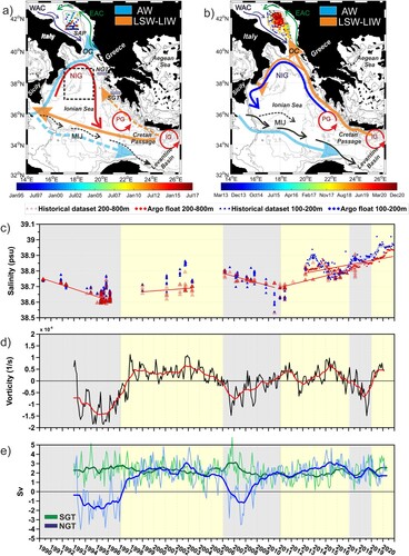
The complex thermohaline circulation of the SAP () is driven by the interaction between different processes: the wintertime dense water formation events that occur through open-ocean convection (Gačić et al. Citation2002); the inflow of fresher water from the northern Adriatic rivers (Vilibić et al. Citation2013) and of dense water produced in the northern Adriatic (Bensi et al. Citation2013); and the inflow/outflow of surface-intermediate/dense water masses from/to the Otranto Channel (Yari et al. Citation2012). Moreover, thermohaline and biogeochemical properties in the SAP are closely related to the periodic reversal (from anticyclonic to cyclonic and vice-versa) of the Northern Ionian Gyre (NIG; Gačić et al. Citation2010, Citation2021; Menna et al. Citation2019; Rubino et al. Citation2020) on a quasi-decadal temporal scale (Civitarese et al. Citation2010; Mihanović et al. Citation2021). NIG reversals affect the water mass distribution among the Eastern Mediterranean sub-basins (Gačić et al. Citation2011; Bessieres et al. Citation2013; Reale et al. Citation2017; Notarstefano et al. Citation2019), in turn influencing the thermohaline properties of the whole Mediterranean on decadal and multi-decadal scales (Gačić et al. Citation2013; Schroeder et al. Citation2017; Menna et al. Citation2022). Changes in the NIG shape and strength occur on interannual scales, responding to large climatic events (e.g. the Eastern Mediterranean Transient) and to the variability of the adjacent sub-basin scale and mesoscale circulation structures (Menna et al. Citation2019; Kalimeris and Kassis Citation2020).

The anticyclonic phase of the NIG brings Atlantic Water (AW) toward the northern Ionian and southern Adriatic ((a)), inhibiting its advection toward the easternmost Mediterranean sub-basins (weakening of the Mid-Ionian Jet; Menna et al. Citation2019). This condition favours the salinity increase in surface and intermediate waters of the Levantine and Aegean seas (Gačić et al. Citation2014; Ozer et al. Citation2017). On the other hand, the cyclonic phase of the NIG brings Surface and Intermediate Levantine Waters (LSW and LIW, respectively) in the northern Ionian and Adriatic basins ((b)), by favouring the direct flow of AW toward the Levantine Basin (strengthening of the Mid-Ionian Jet). This condition leads to a salinity reduction in the Levantine and Aegean Seas (Gačić et al. Citation2011; Reale et al. Citation2017; Menna et al. Citation2019, Citation2022). Salinity content in the surface and intermediate layers of the SAP influences the strength of the winter convection processes (Civitarese et al. Citation2010) and the thermohaline characteristics of the dense water formed during these events (Bensi et al. Citation2016). These dense waters reach the deep/bottom layers of the Ionian Sea (Bensi et al. Citation2016) affecting the thermohaline circulation and the ventilation of the deep Eastern Mediterranean (Mihanović et al. Citation2021). The dynamics of the SAP and of the Northern Ionian are thus intimately interlinked, shaping the decadal variability of the Mediterranean overturning circulation (Civitarese et al. Citation2010; Gačić et al. Citation2013; Vilibić et al. Citation2013).

In recent years, numerous works highlighted strong changes in the salinity distribution of the SAP, emphasising how this variability is linked to the nutrient concentration (Civitarese et al. Citation2010), the plankton abundance/composition (Batistić et al. Citation2019), the presence/absence of fish species of commercial interest (Mauri et al. Citation2021), the fishery activity (Carlucci et al. Citation2016), and hence to the economy of the region. Argo floats and underwater gliders detected an unusual double maximum salinity pattern in the vertical structure in late 2015 and 2016 (Kokkini et al. Citation2018, Citation2020; Mauri et al. Citation2021): the first maximum (S = 38.9) is located at about 50 m depth; the second (S = 38.8) at about 400–500 m. In January 2017, very strong open-ocean convection and the consequent deep mixing (between the surface and 700–800 m of depth) destroyed the double salinity pattern of the previous two years, redistributing high salinities throughout the water column (Kokkini et al. Citation2020; Mihanović et al. Citation2021). This deep mixing event, combined with extremely dry conditions, high evaporation and the inflow of high salinity waters from the northern Ionian in late winter/spring of 2017, contributed to the exceptional high salinity values observed in the Adriatic Sea in 2017 (salinity larger than 39.2 measured by an Argo float in the SAP in the layer 15–40 m; Beg Paklar et al. Citation2020; Mihanović et al. Citation2021).

In this work, we focus on the events that occurred in the Ionian Sea from 2017 that contributed to a very intense salinification process observed in the SAP surface and intermediate layers until 2020. In situ observations, satellite data and model reanalysis are used to describe the main large-scale forcing affecting the recent salinity increase in the SAP.

4.7.2. Data and methods

Salinity data collected by Argo floats in the SAP (2013–2020; CMEMS product Ref. No. 4.7.5) were used in conjunction with historical data (retrieved from the World Ocean Database; Conkright Citation1998; Garcia et al. Citation2018; Ref. No. 4.7.6), to construct a time series over the last 31 years (1990–2020). The vertically averaged salinity values in the SAP were computed in the sub-surface (100–200 m) and intermediate (200–800 m) layers ((a–c)).

Monthly means of the Absolute Geostrophic Velocities (AGV) derived from satellite altimetry data (CMEMS product Ref. No. 4.7.2), available in the period 1993–June 2020 were used to estimate the relative vorticity field, spatially averaged in the region of the northern Ionian Sea (37–39°N and 17–19.5°E; the area selected is the same as used in Shabrang et al. Citation2016; Notarstefano et al. Citation2019; (d)), and the horizontal transport field (defined in Pinardi et al. Citation2019), integrated from 0 m to 100 m depth. Monthly time series of vorticity (black line in (d)) and of the meridional component of the volume transport (light green and light blue lines in (e)) across the SGT and NGT transects (shown in (a)), were filtered using a 13-month moving average (thicker and darker lines in (d,e)) to remove the seasonal variations and to focus on the interannual fluctuations. Transect locations were chosen in order to intercept the pathway of the surface current along the western Greek coast.

Due to data availability issues, yearly means of the horizontal volume transport were computed using the AGV derived from the CMEMS product Ref. No. 4.7.2 in 2017–2019, and those derived from the CMEMS product Ref. No. 4.7.1 in 2020. Velocity vectors associated with the horizontal transport were superimposed on the yearly mean model-derived salinity products (at 153 m depth; CMEMS products 4.7.3 for 2017–2019 and 4.7.4 for 2020), to provide a general overview of the surface dynamics along with the salinity distribution in the Ionian and southern Adriatic ().

Figure 4.7.2. Mean velocities associated with the horizontal volume transport in bins of 0.25°×0.25° derived from satellite altimetry (CMEMS products Ref. No. 4.7.1 and 4.7.2; the product Ref. No. 4.7.1 is an improvement of the product Ref. No. 4.7.2, based on a more accurate Mean Dynamic Topography, currently available from April 2019; for more details see Taburet et al. Citation2019), integrated from the surface to 100 m depth, superimposed on mean salinity patterns (153 m depth; CMEMS products Ref. No. 4.7.3 and 4.7.4) for the years (a) 2017, (b) 2018, (c) 2019, (d) 2020.

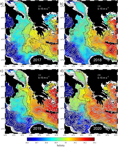
Data from a surface drifter (IMEI 300234065616590) and an Argo float (WMO 6902848) were used to define the pathway of LSW and LIW toward the SAP (; CMEMS product 4.7.5). The water masses sampled in the whole water column of the SAP are shown in the T/S diagram of (d) (CMEMS product 4.7.5).

Figure 4.7.3. Trajectories of (a) drifter IMEI 300234065616590 and of (b) Argo float WMO 6902848 colour-coded by time. (c) Contour diagram of salinity collected by the float WMO 6902848. (d) T/S diagram of the float profiles collected in the SAP coloured by time. CMEMS product Ref. No. 4.7.5.

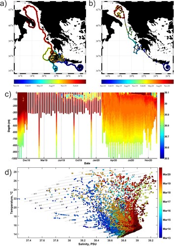
4.7.3. Results and discussion

The analysis of the 30-year time series (1990–2020) shows a positive linear trend of salinity values in the SAP ((c)). During the period 1990–2016, the time series shows the quasi-decadal variability driven by the NIG circulation reversals. The entrance of fresh AW in the SAP during the anticyclonic phases of the NIG leads to a decrease of the mean salinity values both in the sub-surface and intermediate layers while, the inflow of LSW and LIW, during the cyclonic phases of the NIG leads to high salinity values at the sub-surface and intermediate layers ((c)). From 2017 onwards, the mean salinity values increased both at the sub-surface and at intermediate layers, although in 2017–2018, the salinification of the SAP is not supported by the concurrent anticyclonic circulation of the NIG (Grodsky et al. Citation2019; Notarstefano et al. Citation2019), which is expected to favour the inflow in the SAP of less saline water coming from the Western Mediterranean. From 2019 onwards, the NIG reverts to a cyclonic mode favouring the continued increase of salinity, as observed in 2019–2020. The salinity maxima of the historical time series are recorded in 2019–2020 in the sub-surface layer and in 2020 at intermediate depth ((c)).

The inflow of high salinity Levantine origin waters into the SAP in the period 2017–2020 is linked to two main features. The first one is the temporal extension and the intensity of the 2017–2018 anticyclonic NIG phase. The time series of vorticity in (d) shows the NIG inversion from cyclonic (positive vorticity) to anticyclonic (negative vorticity) in 2017. This condition lasts over two years (2017 and 2018), and from 2019 the cyclonic circulation mode is re-established ((d)). This short temporal extension, compared to the previous two anticyclonic events, affects the expected impact on the salinity in the SAP; Mihanović et al. (Citation2021) estimated a lag of 1–2 years between the NIG vorticity reversals and the salinity response in the middle Adriatic. Moreover, the negative vorticity associated with the anticyclonic NIG modes decreases with time showing lower magnitudes in the period 2017–2018 relative to those of the 1990s. Reduced vorticities indicate a weakening of the current field in the NIG, presumably associated with a reduced transport of AW toward the SAP (Gačić et al. Citation2011). The weakening of the NIG current field and the short lifetime of the anticyclonic mode in 2017–2018 concur to maintain the high salinity condition generated in the SAP during the previous cyclonic period (2011–2016; (c)).

The second feature that supports the inflow of Levantine and Aegean origin waters into the SAP in the period 2017–2020 is the presence of an intense northward coastal current along the eastern Ionian coast. This current is a permanent feature in the surface circulation of the Ionian Sea, independent from the circulation mode of the NIG, but it is intensified during a cyclonic mode (Menna et al. Citation2019; Kalimeris and Kassis Citation2020; Menna et al. Citation2021). The meridional components of the volume transport across the SGT and NGT transects ((e)) help to further define the coastal current behaviour, characterised by a marked seasonal variability with occasional reversals during spring and summer, in agreement with the results of Kalimeris and Kassis (Citation2020) and Mihanović et al. (Citation2021). It is always oriented northwards at SGT (positive values of the volume transport, (e)), showing an interannual variability not related to the NIG reversals. Further to the north, at the NGT, the coastal current shows decadal fluctuations correlated with the NIG reversals, with southward transports during the anticyclonic mode (negative values of the volume transport; (e)) and northward transports during the cyclonic mode. In 2017, the reduced strength of the surface current with respect to the previous NIG anticyclonic phases, leads to a temporary weakening of the northward transport at NGT, but not to its reversal. Consequently, transport across the NGT has had an upward trend since 2008 ((e)).

In 2017–2018, the NIG western branch transports low saline AW northward, from the Sicily Channel towards the northern Ionian, up to ∼ 39.5°N ((a,b)). Low saline waters are confined to the interior of the NIG signature, whereas the easternmost part of the Ionian Basin is occupied by high saline water of Levantine and/or Aegean origin. These waters, transported northward from the Cretan Passage along the eastern Greek coast, reach the Adriatic Sea and feed a saltier tongue along the eastern edge of the SAP ((a,b)). In 2019–2020, the northward transport of AW is strongly reduced; the high saline water still feeds the Adriatic Sea following the coastal pathway but also fills the interior of the Ionian Basin, following the cyclonic meander of the NIG ((c,d)).

The coastal pathway along the Greek coast provides a direct link between the Levantine/Aegean basins and the SAP as shown by the horizontal transport and salinity field () and confirmed by the trajectories of drifter IMEI 300234065616590 and Argo float WMO 6902848 ((a,b)), deployed together southeast of Crete in October 2018. Following the path of this coastal circuit, surface and intermediate waters move from the Levantine toward the southern Ionian along the southern Cretan coast, recirculate in the Pelops Gyre and, from there, are redirected northward toward the Adriatic Sea. Moreover, salinity profiles collected by the float show that the Levantine waters following this route have reduced possibilities to mix with the resident waters of the Ionian Sea, retaining very high salinities (larger than 38.9) when entering the SAP in February 2020 ((c)). The highest salinity values (between 39.1 and 39.27) are recorded by the float WMO 6902848 in the period June–September 2020 in the layer 0–50 m. From October 2020, the float moves cyclonically along the SAP border, from west to east ((b)), sampling at the interface between the saltier and warmer waters in the interior of the cyclonic circulation and the colder and less salty waters transported from the northern Adriatic by the WAC ((a,b)). A plume of these northern waters enters in the interior of the SAP reducing its surface layer salinity in November – December 2020. The T/S diagram including all the float profiles available in the SAP, clearly shows the gradual salinification of the whole water column in the period 2013–2020 ((d)). Record-breaking salinities of 39.27 are observed in 2020, slightly higher than those of 2017 (38.24).

These results clarify that the exceptional salinity values observed in the southern and middle Adriatic in 2017 (Beg Paklar et al. Citation2020; Mihanović et al. Citation2021) are part of a SAP salinification process that has continued in the following years, reaching even higher values in 2020. Compared to previous works, mainly focused on the middle Adriatic and on the local forcings, this work highlights the large-scale drivers, taking into account the dynamics of the whole central Mediterranean and demonstrating the unambiguous connection between the Levantine/Aegean basins and the southern Adriatic.

Record-breaking salinity values recorded in the surface and intermediate layers of the SAP in 2020 are the result of a decadal salinification process, that shows a steep increase from 2017, and are a sign of changes in the zonal overturning circulation of the whole Mediterranean. Through deep convection events, the high salinity in the SAP could potentially induce future changes also in the deepest north–south thermohaline cell of the Eastern Mediterranean. The SAP salinification process, with its potential effects on the local biogeochemical cycles, nutrient concentrations and trophic network characteristics, as well as on the larger scale ocean and climate dynamics, is revealed as a key indicator linking many features of the Mediterranean Sea variability.

Section 4.8. Coastal upwelling along the Turkish coast of the Black Sea: Its role in the distribution of the hydrographic properties

Authors: Murat Gunduz, Salvatore Causio, Giulia Bonino, Luc Vandenbulcke, Marilaure Gregorie, Leonardo Lima, Stefania Ciliberti, Mehmet Ilıcak, Ali Aydogdu, Simona Masina, Giovanni Coppini, Nadia Pinardi

Statement of main outcome: Nutrient-rich deep waters of the ocean are carried to the surface by means of vertical transport. This vertical movement is called upwelling. Upwelling along the Turkish coast of the Black Sea is a known oceanographic feature of the Black Sea dynamics. In general, the winds blowing along the coastline are responsible for this vertical movement. Depending on the strength and duration of the upwelling favourable winds, the properties of the upwelled water are also affected. The analysed sea surface temperature both from observation and numerical model results indicate strong inter-annual variability of the upwelling events in the Black Sea. The current paper shows that the main mechanism behind the upwelling along the southwestern coast of the Black Sea is the northerly wind regime called Etesians. The calculated Ekman transport showed that the maximum transport occurs from July to October localised between 31°E and 32°E longitude bands. While upwelling becomes stronger, the SST does not follow this. Correlating the upwelling with the main teleconnection patterns does not give any significant results except for a weak correlation with the North Atlantic Oscillation.

Products used:

Table

4.8.1. Introduction

Nutrient-rich and oxygen-poor waters can rise from the deep ocean to the euphotic layer through an oceanographic process called upwelling. Upwelling is commonly driven by alongshore winds, together with the Coriolis effect, which forces offshore water transport through Ekman Transport (Bakun Citation1990). Due to the nutrient-rich upwelled water, upwelling regions are thus crucial for the global biogeochemical cycles, regulating productivity at a global scale (Pauly and Christensen Citation1995; Bindoff et al. Citation2019). In these regions the growth and reproduction of primary producers (e.g. phytoplankton) form the base of the oceanic food web, leading to enhanced biological/fish production (Garca-Reyes et al. Citation2015; Jacox et al. Citation2015). Upwelling is a critical process for global circulation and climate, as they allow the mixing of water masses from different ocean layers, they modulate to some extent the basin-scale circulation. In coastal regions, they act to link the productive coastal region to the adjacent oligotrophic waters exporting large amounts of organic and inorganic material (Lovecchio et al. Citation2018; Bonino et al. Citation2021).

Two major upwelling regimes exist, i.e. open ocean upwelling and coastal upwelling regions. Open ocean upwelling occurs, for instance, in the equatorial region. The equatorial upwelling is induced by near-surface Ekman Transport divergence caused by the effect of the Coriolis force on trades winds. On the other hand, the major coastal upwelling regions are the Eastern Boundary Upwelling Systems (EBUS) which are located at the eastern side of the subtropical gyres (Pauly and Christensen Citation1995; Chavez and Messié Citation2009). There is a very limited number of known coastal upwelling regions over the Euro-Asian Seas. For example, the upwelling in the eastern coast of the Aegean Sea is responsible for the cold waters along the Turkish coast in the summer (Ciappa Citation2019). The Iberian upwelling system is another important one (Miranda et al. Citation2013) responsible for mesoscale eddies in the region. The eastern coast of the Caspian Sea during summer periods experiences strong temperature drops related to the coastal upwelling processes bringing nutrient-rich waters at the surface ocean layer (Sur et al. Citation2000; Tuzhilkin and Kosarev Citation2005).

The impact of the recent climate change is already seen in the upwelling regions of the world (Bakun Citation1992; Bakun et al. Citation2010; Di Lorenzo Citation2015; Bindoff et al. Citation2019; Bonino et al. Citation2019). Since the upwelling is closely related to the coastal wind regime which is also affected by the global atmospheric circulation pattern, the upwelling characteristic is directly related to climate change (Bakun et al. Citation2010; Bindoff et al. Citation2019). Therefore, it is important to understand the mechanism behind the upwelling and its variability.

In this work, upwelling occurring along the Turkish coast in the southwestern part of the Black Sea is studied. The possible mechanism and the time variations of the Black Sea upwelling have not been very well studied in the past. There is a very limited number of studies on the southern coast upwelling. Sur et al. (Citation1994) have discussed that the possible reason for the upwelling in the Turkish coast of the western Black Sea is the surface divergence of the Rim current based on the evidence of the warm surface coastal water observed one month before the upwelling. In another study, Göktürk et al. (Citation2014) have shown that the Etesian wind regime dominating the general wind pattern over the Sea is the possible reason for this coastal upwelling in the Black Sea.

This study utilises observations and model results from the Black Sea eddy-resolving reanalysis (Lima et al. Citation2021) delivered in the framework of the Copernicus Marine Environment and Monitoring Service (CMEMS) to better understand the mechanism behind the upwelling over the southwest coast of the Black Sea. The calculated upwelling index (Bakun Citation1973) by using the Ekman transport will help to evaluate the spatial and temporal variation of the upwelling events. Since there is not enough literature in the study region, the current study will fill this gap by providing the information about dynamics of the upwelling in the Black Sea.

4.8.2. Data and methods

There are quite a number of meteorological observations along the Turkish coast of the Black Sea. , the top panel shows the location of the available meteorological station observations obtained from the Turkish Meteorological Service (product ref. 4.8.2). Sea Surface Temperature (SST) and zonal and meridional winds are recorded at these stations. The station data have one hourly frequency covering the period from 2013 to 2020. The Black Sea reanalysis is obtained from CMEMS (product ref 4.8.1; Lima et al. 2020, Citation2021). The reanalysis model domain covers the whole Black Sea except the Azov Sea. The model has approximately 3 km horizontal grid resolution with 31 vertical levels. The numerical model is based on the NEMO version 3.6 and forced with the ECMWF-ERA5 0.25 degree at 1 hourly atmospheric forcing. The whole available in-situ and satellite altimetry observations are assimilated using the OceanVar, a variational data assimilation scheme (Dobricic and Pinardi Citation2008; Storto et al. Citation2011). The variables used in this study are daily mean SST.

Figure 4.8.1. Top panel: Locations of the available meteorological stations (product ref 4.8.3) and the orange dot is the location of the sample time series. Middle panel: Time series of SST from sample observation (black stars, product ref 4.8.2) and reanalysis ocean model (red lines, product ref 4.8.1) for the all-available period 2013–2020. Bottom panel: Time series of SST from observation (black stars, product ref. 4.8.2) and reanalysis ocean model (red lines, product ref 4.8.1) for only 2018. Right column: Model SST bias for the all stations from west to east shown in the top panel.

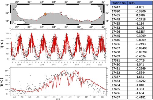
The classical upwelling index is mostly known as the Bakun index (Bakun Citation1973) and is basically linked to the Ekman volume transport. The zonal and meridional component of the Ekman transport (m²/s) is calculated by using the below equations where $τ$ is the wind stress obtained from the ECMWF-ERA5 reanalysis (product ref 4.8.3) interpolated on the ocean model grid, $ρ_{o}$ is the density of the seawater, and f is the Coriolis parameter. $U_{e k} = τ_{o}^{y} / ρ_{o} f$ $V_{e k} = - τ_{o}^{x} / ρ_{o} f$

The cross-shore Ekman transport (Cropper et al. Citation2014) which is also known as upwelling index (UI) is calculated by the below formula. The $θ$ is the angle between coast and the equator. Upwelling-favourable conditions are satisfied if this variable is negative. $Q_{c r o s s} = U_{e k} \sin (θ) - V_{e k} \cos (θ)$

The Ekman pumping is related to the curl of the wind stress, and it is calculated by the below equation. The wind stress is on the ocean model grid resolution and the closest value to the coastline is chosen. $W_{e} = c u r l (τ) / ρ_{a} f$

The Northern Hemisphere teleconnection indices used in this study were obtained from product ref. 4.8.4.

4.8.3. Results and discussion

SST data from the meteorological stations and the ocean model reanalysis were analysed to better understand the possible trend of the upwelling along the Turkish coast of the Black Sea. The top panel of shows the locations of the meteorological stations. An example of the SST time series of a station (biggest orange dot) is shown in the middle panel of (black stars) along with the SST results from the Black Sea reanalysis (red lines, product ref. 4.8.1). The spike-like patterns seen as a drop in temperature are the upwelling events. It is clear that the intensity and the number of upwelling events show strong inter-annual variability. A zoom of the above time series for the specific year 2018 is shown in the bottom panel of . The upwelling event can stay 5–10 days as seen in the August 2018 event. The model bias is shown on the right panel of as a table for all meteorological stations. In general, the reanalysis agrees with the observation. The model bias is close to zero around the upwelling region suggesting that the model manages to catch the upwelling events. It is clear that the model temperature is warmer (bias is always negative) than the observations as seen in the bias statistics.

shows the June to September averaged mean surface temperature (black lines) and cross shore Ekman transport (blue lines) for the selected stations from west to east shown in the top panel. The strong negative correlation between the SST and cross shore Ekman transport is evident in the upwelling stations suggesting that the main mechanism for the upwelling along the Turkish coast of the Black Sea is Ekman transport (wind). The highest correlation is observed in the fourth station (with a correlation coefficient value of r = −0.77) which is known as the centre of the upwelling region.

Figure 4.8.2. Top: Locations of the six stations around the upwelling region. Time series of June to September averaged mean surface temperature (black line) and cross-shore Ekman Transport (blue line) for the above six stations from left to right. The correlation coefficient between SST and Ekman transport is given by p. The trends are shown with the dashed lines.

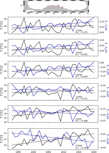
The correlation between SST and Ekman transport decreases outside of the upwelling region. It is interesting to note that, while in all of the upwelling stations Ekman transport shows a positive trend (strengthening of upwelling) there is no clear trend (very weak positive trend) of SST in the upwelling region. It was expected that intensification of the upwelling could result in decrease of the SST at the upwelling region. However, it could be speculated that the recent warming of the Cold Intermediate Layer (CIL) where most of the upwelling waters comes from could affect the warming of the upwelled waters. This situation completely changes outside of the upwelling region with a strong negative trend of the Ekman transport and the quite positive trend of the SST as seen in the last two time series of the . The reason for the intensification of the downwelling-favourable conditions and warming outside of the upwelling region needs to be further examined, but it is beyond the scope of this study.

The mean wind stress magnitude and direction averaged from 1980 to 2020 over the Black Sea is shown in , panel (a). The wind stress along the southwestern coast of the Black Sea is suitable for the upwelling, this northerly wind regime is called as Etesian winds (Rusu et al. Citation2018). The spatial extent and time variability of the upwelling index is shown by the Hovmöller diagram of the mean total Ekman per bin of longitude in , panel (b). There is a clear contrast of the upwelling (positive total Ekman) and downwelling (negative total Ekman) regimes divided at the centre of the Black Sea (approximately at 33°E). The maximum transport is seen from July to October between the longitudes of 31°E and 32°E. The longitudinal averaged coastal upwelling (V_ek), Ekman pumping (W_e), coastal upwelling + Ekman pumping (tot Ek) is shown in , panel (c). The positive transport indicates the occurrence of upwelling. The maximum peak seen at around 31.5 °E is compatible with the results of the Hovmöller plot and corresponds to the centre of the upwelling region. Ekman pumping value is quite lower than the Ekman transport for all longitude section and it is even much lower at outside of the upwelling region. The possible relationship between the upwelling and the large-scale atmospheric teleconnection pattern was also investigated by calculating the correlation coefficient between Ekman transport and teleconnection indices. However, there is no significant correlation except with the weak correlation with the North Atlantic Oscillation (NAO).

Figure 4.8.3. (a) Averaged wind stress. (b) Hovmöller plot of mean total Ekman transport per bin of longitude per month. (c) zonal Ekman transport component (V_ek), Ekman pumping (W_e), coastal upwelling + Ekman pumping (tot Ek) along the Turkish coast (longitude).

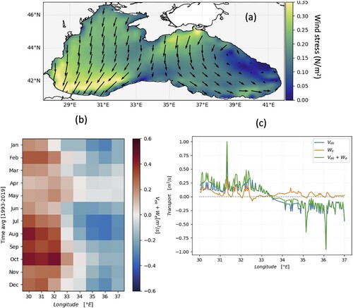
4.8.4. Conclusions

The inter-annual variability and possible mechanism behind the upwelling along the Turkish coast of the Black Sea are studied by using meteorological station data and ocean circulation model reanalysis results. It is shown that the upwelling intensity and duration show strong inter-annual variability along the Turkish coast of the Black Sea, which are evident both in the observation and the long-term Black Sea reanalysis. The reanalysis SST gives more detailed information about the spatial and temporal extent of the upwelling by providing longer time scale of the ocean compared to the limited number of SST observations on the Turkish coast. The upwelling is mostly affected by the wind regime of the region. However, in some cases, even when there are no upwelling favourable winds, the SST shows a strong decrease, which needs to be further explained.

Considering the fact that the upwelled waters come from subsurface where the Cold Intermediate Layer (CIL, which is the water masses with a temperature less than 8 degrees) is also located, the recent diminishing of the CIL (Stanev et al. Citation2019; Lima et al. Citation2021) probably affects the upwelled characteristics over the study region and this also needs further study.

The Classical upwelling index (Bakun index) based on Ekman transport ignores the along-shore transport of water. In a further study, a more advanced upwelling index such as the Coastal Upwelling Transport Index (CUTI) (Jacox et al. Citation2018) considering the along-shore wind stress and geostrophic current could be applied.

The transport of biogeochemical properties over the upwelling region is a critical process and needs to be better evaluated. In this regard, another upwelling index called Biologically Effective Upwelling Transport Index (BEUTI) (Jacox et al. Citation2018) considering the nutrient concentration in the mixed layer depth could give more detailed information on the biogeochemical exchange process in the region.

Supplemental material

Supplemental Material

Supplemental Material