Using eddy-covariance to measure the effects of COVID-19 restrictions on CO₂ emissions in a neighborhood of Indianapolis, IN

Abstract

Eddy-covariance (EC) flux measurements in Indianapolis were used to quantify the impact of the COVID-19 lockdown on CO and CO₂ emissions from a highway and a suburban neighborhood. CO₂ fluxes were measured for 6 weeks pre-lockdown (January 22, 2020–March 3, 2020) and during lockdown (March 25, 2020– May 5, 2020) using EC instrumentation at 41 m AGL. Fossil fuel CO₂ emissions (CO₂ff) were estimated by calculating eddy diffusivity to obtain CO flux and then scaling by the CO:CO₂ff emissions ratio (R_CO). Flux measurements segregated by wind direction were compared to hourly emissions from the 2020 Hestia inventory model. The lockdown CO₂ff average weekday emissions from the highway estimated by EC decreased by 51.5 ± 10.9% (11.2 ± 2.2 µmol m⁻² s⁻¹) compared to pre-lockdown, similar to Hestia’s estimate 56 ± 7% (12 ± 1 µmol m⁻² s⁻¹). The EC measurements detected a significant (2.2 ± 0.7 µmol m⁻² s⁻¹) but smaller magnitude decrease in CO₂ff emissions from the suburban neighborhood. The daily cycles of CO₂ff emissions were significantly correlated with Hestia estimates from the highway but not from the suburbs. This study demonstrates that EC flux towers and high-resolution inventory models in regions with mixed and spatially heterogeneous sources can quantify abrupt changes in sector- and source-specific CO₂ fluxes.

Keywords:

• Flux
• disaggregation
• coronavirus
• footprint
• Hestia
• INFLUX
• Indiana

Introduction

Measurement strategies that can accurately quantify changes in anthropogenic emissions are needed to evaluate efforts to curb greenhouse gas emissions. The lockdowns enacted due to the outbreak of the COVID-19 (Coronavirus disease 2019) pandemic provide an opportunity to test strategies for monitoring changes in emissions, since vehicle traffic and its associated emissions dropped significantly during the pandemic [1–3]. Other emissions sectors, such as industry, power production, and public buildings also decreased their daily global CO₂ emissions according to one inventory study, while daily global residential emissions went up slightly [4]. Fossil fuel-sourced CO₂ emissions (referred to henceforth as CO₂ff emissions) as well as other pollutant emissions have been demonstrated to have decreased during pandemic-related lockdowns [4–6]. Studies of primary air pollutants found that government lockdown orders catalyzed significant decreases in carbon monoxide, nitrogen oxides, and particulate matter [7,8].

A limited number of studies have used atmospheric data to quantify changes in emissions due to COVID-19 restrictions. One study used satellite data from the GEOS/OCO-2 atmospheric carbon monitoring system to analyze the CO₂ emission patterns of various countries during 2020 [9]. The results showed increases and decreases in average country-wide emissions that agreed loosely with inventory data and the slackening and tightening of COVID restrictions [9]. The study was significant because it demonstrated how inventory data and atmospheric data could be used to conclude how COVID-19 affected emissions and gauge the accuracy of both monitoring systems. Some urban-scale greenhouse gas (GHG) measurement networks have demonstrated city-level emissions changes due to COVID-19 restrictions [7,8]. The Air Quality Monitoring Network of the Santiago Metropolitan Area measured concentrations of NO_x, CO, O₃, and other pollutants [7]; particulate matter data collected by the local environmental protection agency of Milan was used to monitor COVID-related changes in emissions of C₆H₆, CO, SO₂, and others [8]. To observe changes in emissions caused by the COVID-19 lockdown in six North American cities (Boston, Indianapolis, Los Angeles, Salt Lake City, Toronto, and the Baltimore/D.C. metro area), six different metrics were used: amplitude of the diurnal cycle, vertical gradients, enhancements above the background, temporal variances, and enhancement of the CO₂:CH₄ ratio [10]. This study’s goal is to build on the successes of these previous studies by using EC measurements to better quantify COVID-19 emissions reductions at a smaller scale.

EC flux measurements, the primary measurement method for this research paper, effectively monitor CO₂ fluxes at high spatial and temporal resolution in natural and urbanized environments [11,12]. EC flux measurement towers monitor all CO₂ emissions sources and sinks within its footprint, making it an ideal tool for monitoring emissions in specific regions of interest. The strategy has been deployed in many cities for various purposes such as testing the accuracy of other urban-scale measurement methods or comparing with local activity data to determine dominant sources and sinks in the area [13–15].

EC towers yield data that can be combined with other measurements to better quantify human emissions. For instance, one can use EC measurements along with trace gases to disaggregate CO₂ sources. A study in Tokyo, Japan used O₂ and CO₂ mole fractions, and an inventory model in tandem with CO₂ flux measurements to estimate daily cycles for emissions from gas fuels, liquid fuels, and human respiration [16]. They observed O₂:CO₂ ratios, and since these ratios are different for gas and liquid fuels, they could use these ratios and inventory data for source attribution [16]. Our study builds on previous EC studies like the ones in London and Tokyo [16] by using molar concentration measurements above and below the flux measurement device to disaggregate CO₂ measurements into their fossil fuel and biogenic components.

EC has been helpful in examining the impact of COVID-19 restrictions on CO₂ emissions. EC measurements have shown that CO₂ flux in Yoyogi, a residential area in Tokyo, Japan, dropped by about 20% in April and May of 2020 when the Japanese government encouraged everyone to stay at home reducing public activities [17]. A study in Vienna, Austria, with EC measurements 144 m AGL from 2018 to 2020 found that weekly mean CO₂ fluxes for north-westerly winds during the city’s 2020 lockdown were 64% lower than corresponding means in 2019, a greater reduction than was observed when wind blew from less urbanized directions [18]. A network of European urban EC measurements of total CO₂ flux observed large emissions reductions in most cities that were a function of the severity of COVID-19 restrictions imposed [19]. These restrictions included closing schools and businesses, banning of social gatherings, and stay-at-home orders [19]. Dividing tower footprints into different sections by wind direction and identifying the dominant emission sources and sinks in each section provided insight into how different emissions sectors were affected [19]. Non-residential areas experienced the greatest emissions reductions during lockdowns [19].

A combination of flux footprint analyses and multi-gas tracers can further improve our ability to identify flux patterns, sources, and sinks in heterogeneous urban settings. Wu et al. presented a method for decomposing the anthropogenic and biogenic fluxes using CO:CO₂ff emissions ratios (R_CO) and segregating the fluxes in space using flux footprints [20]. Measurements of CO and ¹⁴CO₂ can be used to quantify a region’s R_CO, as was done for Indianapolis [21]. With this ratio, CO and CO₂ gradient measurements, and EC measurements of the total CO₂ flux, one can separate the biogenic and CO₂ff contributions from the total flux. This study uses this approach to study the impact of COVID-19 restrictions on CO₂ff emissions.

The goal of this study was to use EC CO₂ flux and CO₂ and CO mole fraction measurements to quantify the change in emissions from fossil fuel sources that occurred due to the COVID-19 lockdown in Indianapolis, Indiana. The hypothesis tested was that CO₂ff emissions from traffic dropped significantly during Indianapolis’ pandemic-induced lockdown. It was also predicted that the reduction in CO₂ff emissions would be evident in the disaggregated EC fluxes and the Hestia emissions inventory. Another objective was to search for evidence of a change in R_CO during lockdown since traffic and other sources of CO₂ff were likely affected by the lockdown. The emissions changes from the pandemic lockdown provide an opportunity to test our ability to quantify emissions changes that might take place as purposeful emissions management policies and technologies are implemented and to establish methodologies that can be deployed to study urban metabolism at neighborhood resolution.

Materials and methods

Locations and methods for data acquisition

The EC measurement site used for this research is AmeriFlux site US-INg in the INFLUX mole fraction monitoring network [22,23]. Its position in a medium-sized city during the COVID-19 lockdown provided an excellent opportunity to determine our ability to extract source-specific emissions changes using the multi-gas flux tower methodology previously demonstrated at INFLUX [24]. The ongoing Indianapolis Flux Experiment (INFLUX) has applied several methods of monitoring CO₂ emissions in an urban environment useful for monitoring events such as COVID-19-induced lockdowns [20]. These methods include airborne [25] and tower-based [26] measurements of GHGs. All towers continuously measure CO₂ mole fractions, some also measure CH₄ and CO, and a subset of the towers measure at 2 to 4 different altitudes [23,27].

The observations used for this experiment were obtained from US-INg, located approximately 175 m to the west of a highway (Figure 1). US-INg’s CO₂ flux measuring equipment was added in April of 2019. Traffic on the highway, a primary arterial encircling the city of Indianapolis, was expected to be a primary source of anthropogenic GHG emissions within the flux footprint of the tower. To the west of US-INg is a suburban neighborhood dominated by houses with an average height of 5 m and vegetation in the form of deciduous trees with an average height of 6 m. To the east, towards the highway, there is little vegetation and few buildings. The average building height from the east is 6 m. Characteristics of US-INg such as building and vegetation height and landcover type/percentage are listed in Table 1. LiDAR data from the Marion County 2016 LiDAR project were used to estimate these roughness elements [28]. A cavity ring-down spectrometer (Picarro, Inc., model G2401) at the base of the tower measured the mole fractions of CO₂ and CO in air drawn down in sampling tubes from 21 and 58 m AGL and calibrated to the WMO X2007 and X2014A scales respectively [27]. Mole fraction data, collected at 2-sec temporal resolution, were reported as hourly means [27]. Compatibility of the INFLUX network was assessed via co-located NOAA flask systems and round-robin type testing using NOAA-calibrated tanks, indicating compatibility of 0.18 ppm CO₂ and 6 ppb CO [21]. EC flux measurements were collected at 41 m AGL using an open path CO₂/H₂O flux sensor (Licor, Inc., model LI7500A) and a sonic anemometer (Gill Instruments Limited, WindMaster 3D). Fluxes were calculated with the EddyPro software package [29]. We selected a 30-min averaging period and used a block-averaging detrend [30,31], then aligned the x-axis with the mean streamline using a double rotation [31,32]. The Webb, Pearman, and Leuning density correction was applied to CO₂ fluxes measured by the open path sensors [33,34], and the methods of Vickers and Mahrt were used to despike the high frequency data before computation [35]. The half-hourly measurements of flux, wind direction, and wind speed collected at 41 m AGL were averaged in 1-h blocks to compare them with the hourly mole fraction data from 21 and 58 m AGL.

Figure 1. Image of US-INg’s location relative to the highway to the east and the Forest and suburban neighborhood to the west. The image also includes an approximation of the tower’s footprint during daylight and nighttime hours, made using Kljun et al. footprint model [43].

Table 1. Characteristics Of US-INg. The domain covers 2 square kilometers centered around US-INg, divided into Eastern and Western halves.

	Population density (people mi^-2) [50]	Local climate zone [51]	Avg building height (m)	Avg vegetation height (m)	Displacement height (m)	Building cover (%) [52]	Vegetation cover (%) [52]
West	2,000–5,000	6	5	6	2.0	11	22
East	2,000–6,500	E	6	5	1.0	12	12

(Cont.).

	Building cover (%) [52]	Vegetation cover (%) [52]
West	11	22
East	12	12

* The footprint of tower 7 encompasses all or part of several census tracts. The number here represents the range of population densities of the different tracts.

The contribution of storage to the total CO₂ flux was estimated using (1) $$F_{\mathit{\text{storage}}}=\frac{\rho }{M_{\mathit{\text{air}}}}{\int }_0^{\mathit{\text{Zr}}}\frac{\partial \overline{c}}{\partial t}\mathit{\text{dz}}$$(1) where $\partial \overline{c}$ is the change in molar concentration (either CO or CO₂) between the following and previous hour, ∂t is the time elapsed between those two measurements (7200s) and zr is the height of the EC measurement, in this case 41 m AGL [36]. This estimate assumes that the molar concentration measured at 21 m AGL represents the column average from the ground to the EC flux inlet. The resulting kinematic flux (ppm m s⁻¹) was converted to µmol m⁻² s⁻¹ for CO₂ and nmol m⁻² s⁻¹ for CO by multiplying by air density (ρ) in unites of kg m⁻³ measured at 41 m AGL and dividing by an air molar mass (M_air) of 28.96 kg kmol⁻¹, then finally multiplying by a factor of 1000 to convert kmol to mol.

Extreme values were screened from the flux record. CO₂ turbulent fluxes outside the range of −20 to 200 μmol m⁻² s⁻¹, latent heat flux outside the range of −50 to 500 W m⁻², or sensible heat flux below −200 W m⁻² were removed. These values, likely caused by either sensor malfunctions (e.g. moisture on the sensors) or a lack of stationary turbulence during the period of the flux calculation, were considered unreasonable given the location of the tower and the time of year. Measurements when friction velocity measured by the sonic anemometer was 0.15 m s⁻¹ or less were excluded as well, since analyses of fluxes suggested that weak mixing below this threshold value led to decoupling of the turbulent flux at 41 m from the surface. Decoupling can lead to smaller flux magnitudes [15]. Weekend hours were also removed since human activity such as vehicle use differs greatly between weekends and weekdays and would be affected differently by lockdown measures.

Flux measurements were separated into two sectors based on wind direction: easterly winds (0°−180°) and westerly winds (180°−360°), referred to from here on as the east sector and the west sector. Flux measurements were further segregated into two time periods, pre-lockdown and lockdown. The lockdown period (March 25–May 5) captured six full weeks of decreased activity according to Google Mobility data, which reports the percent reduction in Google users’ trips to various categories of locations such as workplaces and public transit stations compared to a 5-week period at the beginning of the year [1]. The beginning of the lockdown period coincides with the first full day of COVID restrictions including a state-wide stay-at-home order enacted by the Indiana Governor [37]. January 22–March 3 was a full 6-week period before the activity levels began to drop, ending three days before the first confirmed case of COVID-19 in Indiana was announced [1,37]. The period in between had a sharp decrease in activity that did not level out until the beginning of the selected lockdown period (Figure 2); hence, it was excluded from our analysis [1]. Activity levels slowly increased over the 6-week lockdown but were still well below pre-lockdown activity levels by the end of the period [1]. According to the Oxford COVID-19 Government Response Tracker Stringency Index, which scored government responses to COVID-19 based on criteria such as school/workplace closures, stay-at-home orders, etc., the state of Indiana had a weighted average score of 3.7 during the pre-lockdown period and a score of 65.2 during the lockdown period [38].

Figure 2. Average percent reductions in google mobility data relative to baseline levels in Marion County, Indiana, separated into categories based on the type of destination of the user [1]. Blue circles represent reduction in trips to places of work, red vertical lines represent mobility reduction to users’ homes, pink crosses represent mobility reduction to public transit stations like bus stops and metro platforms, the black stars represent mobility reduction to restaurants, shops, theaters, etc., and the green diamonds represent mobility reduction to grocery stores, pharmacies, specialty food stores, etc [1]. The baseline level is the median value from the period between January 3 and February 6 for each day of the week [1]. The tick marks on the x-axis show the end of the pre-lockdown period (March 3), the beginning of the lockdown period (March 25), and the ending of the lockdown period (May 5).

Disaggregating CO₂ flux into CO₂ff and CO₂bio

To disaggregate the EC flux measurements into fossil fuel emissions and biological emissions (e.g. plant life and human respiration), it was necessary to select an appropriate R_CO value. The year-round, city-wide average of R_CO in Indianapolis has been found to be approximately 8 ppb ppm⁻¹ using ¹⁴CO₂ flask measurements with CO in-situ observations [21]. This provides a baseline value of R_CO for flux disaggregation. However, this value may have changed since 2014. It is also possible that the R_CO for the flux footprint around US-INg from February to April is different from the city-wide year-round average R_CO.

Data collected from easterly winds were used to test for variations in the local R_CO value during the pre-lockdown and lockdown periods of 2020. We assume in this analysis that the fluxes from the east are dominated by fossil fuel emissions and that biological fluxes are negligible. Vertical differences in mole fractions of CO (ΔCO) and CO₂ (ΔCO₂) between 21 and 58 m AGL were examined when the wind blew from the east and good quality EC flux data were present. A linear regression for ΔCO₂ versus ΔCO was performed and the resulting slope was used to estimate the local R_CO value [39]. The linear fit used a 500-iteration Monte Carlo method to perform a Deming fit, thus accounting for uncertainty in the CO and CO₂ molar fractions [39]. This method yields a slightly different result every time, so it was repeated 100 times to get a range of likely estimates for R_CO and R_CO uncertainties. To determine if R_CO changed due to COVID-19’s impacts on traffic, this analysis was performed on ΔCO₂ and ΔCO data during the pre-lockdown and lockdown period, with these analyses broken down further into daylight hours (8am − 5 pm) and nighttime hours (6 pm–7am).

This approach for estimating R_CO assumes that CO₂ fluxes from the eastern sector are entirely due to fossil fuel emissions. This is not entirely true since there is some vegetation and human respiration. There are certainly biological CO₂ fluxes to the west of the tower. The R_CO value from Turnbull et al. (2014) [21], 8 ppb ppm⁻¹ was used in flux disaggregation since that value was found through ¹⁴CO₂ analysis which requires no assumptions about the biological CO₂ fluxes, while the estimate of R_CO using molar fractions from US-INg was conducted as a means of observing relative changes in R_CO due to the lockdown and gauging if the city-wide average R_CO from Turnbull et al. applies to the area directly around US-INg.

The next step of the analysis was to isolate CO₂ff fluxes from the total CO₂ flux. This may not have been essential when winds were blowing from the east due to the expected dominance of fossil fuel sources in that direction, but this was essential for the west sector where the urban forest lay. We used the method described in Wu et al. to estimate CO₂ff emissions [20]. Using an analogue of Fick’s First Law of Diffusivity, (2) $$K=-\frac{F_{{\mathit{\text{CO}}}_2}}{{\nabla \mathit{\text{CO}}}_2}$$(2) we used the CO₂ mole fraction vertical gradient ($\nabla$ CO₂) and the measured CO₂ total turbulent flux (F_CO2) measured by US-INg to compute the eddy diffusivity (K) each hour [20]. Eddy diffusivities of absolute values greater than 5000 µmol m⁻¹ s⁻¹ppm⁻¹ were deemed unrealistic and discarded. The median and standard deviation (σ) of K for the pre-lockdown and lockdown periods were calculated, and K values 3.5σ from the K median were additionally removed as outliers. The eddy diffusivity and the CO vertical gradient were combined to estimate the CO turbulent flux, F_CO, via (3) $$F_{\mathit{\text{CO}}}=-K\nabla \mathit{\text{CO}}.$$(3)

R_CO (8 ppb ppm⁻¹) was then used to estimate the turbulent CO₂ff flux (F_CO2ff), (4) $$F_{{\mathit{\text{CO}}}_2\mathit{\text{ff}}}=\frac{F_{\mathit{\text{CO}}}}{R_{\mathit{\text{CO}}}}.$$(4)

Applying the R_CO to the estimated CO storage was used to estimate CO₂ff storage which was added to the turbulent flux to yield total CO₂ff emissions. Biological CO₂ fluxes were estimated by taking the difference between the total CO₂ flux and the total CO₂ff emissions. After disaggregation, the median and standard deviation of CO₂ff emissions for both periods were calculated. The remaining outliers, values more than 3.5σ from the median CO₂ff value, were removed from the analysis. These extreme values occurred when the vertical difference in CO₂ mole fraction approached zero, and the decomposition Equation (2)(2) $$K=-\frac{F_{{\mathit{\text{CO}}}_2}}{{\nabla \mathit{\text{CO}}}_2}$$(2) became unstable. This analysis was performed for the east sector to analyze highway (US Interstate 495) and commercial development emissions and the west sector to analyze emissions from the urban forest and the neighborhood beyond.

Analysis of results and comparison to Hestia

Average CO, CO₂, and CO₂ff fluxes for each hour of the day were calculated for the pre-lockdown period (January 22–March 3) and the lockdown period (March 25–May 5), and the estimated uncertainty was the standard error of each average. CO₂, CO, and CO₂ff flux averages for the whole period were estimated by taking the average of the 24-hourly averages for each period; this way, the average values are not biased towards hours of the day with more datapoints. Uncertainty was estimated by propagating hourly average errors. The lockdown average was subtracted from the pre-lockdown average for each sector to estimate the magnitude of the changes in flux and percent change. Uncertainty in the changes in flux magnitude and percent was found by propagating the standard error of each average using the additive formula for magnitude and multiplication formula for percent change. To evaluate the importance of the R_CO value to the calculated flux averages, the disaggregation process was repeated numerous times using a range of R_CO values, 6 ppb ppm⁻¹ to 8 ppb ppm⁻¹ value.

The tower-based results were then compared to the Hestia bottom-up emissions data product for Indianapolis. The inventory model Hestia was developed for Indianapolis to provide a high spatial and temporal resolution CO₂ff emissions product that is complementary to atmospheric flux quantification methods [26]. Hestia quantifies carbon emissions at the building/street scale by collecting and merging various data sets, including direct flux measurements, fuel statistics, building attributes, and traffic monitoring [40]. The individual sectors described by Hestia are Onroad, Commercial, Residential, Airport, Electricity Production, Rail, and Nonroad [40]. Version 3.2 Beta of Hestia was used to model emissions in Indianapolis in 2020 at 20 m × 20 m resolution over a 4 km × 4 km domain centered around US-INg [40,41,42].

US-INg’s flux footprint, the region that the tower monitors, changes depending on atmospheric conditions so for an accurate comparison between Hestia data and US-INg data, it is important to account for changes over time in the flux footprint. Hourly averaged measurements of wind speed, friction velocity, Obukhov length (L), wind direction, and the standard deviation of lateral velocity fluctuations at US-INg and hourly boundary layer height from ERA5 reanalysis were used to estimate the flux footprint model at 2 m spatial resolution for each hour [43,44]. The displacement height (z_d) and roughness length (z₀) were estimated during neutral conditions (|z_r/L| < 0.1) by fitting measured windspeeds to the logarithmic wind profile [45]. We separate wind directions into 10° bins and then use a Nelder-Mead algorithm to estimate z_d and z₀ by minimizing the residual sum of squares between windspeed observations and the logarithmic wind profile [46]. The final values of displacement height, used in the footprint analysis, were 2 m from the west of the tower (180°−360°) when winds blew over the urban forest and 1 m from the east (0°−180°) when winds blew over the highway. Values for z₀ were roughly consistent with wind directions (0.11 m) but not used in the footprint analysis since the footprint model can use mean wind speed instead which was being actively measured by US-INg.

Hestia and the flux measurements were compared using these flux footprints. Hestia emission estimates were weighted by the flux footprints to estimate the CO₂ff emissions that were observed at the tower. The 2 m resolution flux footprints output by the model needed to be re-gridded for the borders to match those of the Hestia cells because the borders of Hestia grid cells lie in the middle of the footprint grid cells. To do this, the cells were duplicated in the x and y direction, which can be done because the cell values represent a weighting per area, resulting in a 1 m-by-1m grid. Then, each footprint ($f$) cell was multiplied by the corresponding Hestia emissions cell and the product cells were summed together, resulting in the total turbulent flux ($F_H$) as described by Wu et al. [20]: (5) $$F_H=\sum _{i=1}^R{Q}_H(x_i,y_i)f(x_i,y_i)\mathit{\text{δxδy}}$$(5) where $Q_H$ represents the Hestia emissions for the given hour and R is the flux footprint domain. The resulting $F_H$ was used for the eddy covariance to inventory comparison.

These footprint-matched hourly Hestia estimates were broken up into period and wind direction in the same fashion as the EC flux measurements, and hours that were removed from US-INg analysis were also removed from Hestia analysis to ensure that the same hours were being compared between the two datasets. Then hourly weekday averages and averages for the whole pre-lockdown and lockdown period were calculated using the same methods used for the US-INg data. Standard errors are estimated similarly, representing uncertainty introduced by the footprint calculations.

Results

Emissions reductions by wind sector

Fluxes from the west are relatively small given the lack of large anthropogenic sources and the generally dormant state of the biosphere at this time, but changes in fluxes with time can be detected. In the lockdown period for the west sector, the total CO₂ flux’s positive morning peak is smaller and earlier than the pre-lockdown period (5 am LST vs. 8 am LST) and hourly averages are consistently negative for part of the afternoon, suggesting net photosynthetic uptake (Figure 3(a)). Average weekday hourly CO₂ff emissions during pre-lockdown and lockdown are small (between −7 and 8 µmol m⁻² s⁻¹) and appear to oscillate around zero, likely showing the limits of our measurement precision for 1.5 months of observations from one wind sector (Figure 3(d)). Hourly CO fluxes are lower during lockdown for most daytime hours (Figure 3(b)), yielding small decreases in CO2ff emissions for most hours (Figure 3(c)).

Figure 3. Average hourly weekday emissions observed when winds coming from the west sector (a–d) and the east sector (e–h). The pre-lockdown fluxes are in red and lockdown period fluxes are in blue. The R_CO used to extrapolate from CO to CO₂ff for the data in these graphs is the value from Turnbull et al. [21]. Error bars represent standard error.

Comparison between the pre-lockdown and lockdown average emissions found some reduction in total CO₂ (3.8 ± 0.6 µmol m⁻² s⁻¹, 71.3 ± 13.1%) and CO₂ff emissions (2.2 ± 0.7 µmol m⁻² s⁻¹, 79.1 ± 27.8%) between the two periods (Table 2). A two-sample t-test between pre-lockdown hourly CO₂ff fluxes and lockdown hourly CO₂ff fluxes indicated a significant reduction in the average using the p < 0.05 threshold. There is some reduction in average CO₂ fluxes from biological sources (CO₂bio) west of US-INg (1.6 ± 0.3 µmol m⁻² s⁻¹, 61.4 ± 30.4%) (Table 2), likely due to the increase in photosynthetic uptake in the day during the lockdown period (Figure 3(d)).

Table 2. Reductions in average fluxes from pre-lockdown to lockdown (Δ µmol m⁻² s⁻¹) and percent reductions shown in parentheses (Δ%). Percent reduction is defined here as 100*|(pre-lockdown average – lockdown average)/pre-lockdown average|. Average fluxes are computed by averaging the average hourly fluxes of each period. An R_CO value of 8 ppb ppm⁻¹ was used for flux disaggregation [21]. Uncertainties are standard errors of the mean values.

Emissions source	Avg. westerly reductions Δ µmol CO2 m^−2 s^−1 (Δ%)	Avg. Easterly Reductions Δ µmol CO2 m^−2 s^−1 (Δ%)
Total CO2	3.8 ± 0.6 (71.3 ± 13.1%)	12.3 ± 1.9 (47.5 ± 8.0%)
CO2ff	2.2 ± 0.7 (79.1 ± 27.8%)	11.2 ± 2.2 (51.5 ± 10.9%)
CO2bio	1.6 ± 0.7 (63.0 ± 30.7%)	1.1 ± 1.6 (26.2 ± 38.8%)
Hestia (CO2ff)	4.4 ± 0.3 (63 ± 4%)	12 ± 1 (56 ± 7%)

Total CO₂ fluxes (Figure 3(e)) are highly correlated with CO fluxes (Figure 3(f)) showing the dominance of CO₂ff emission (Figure 3(g)) from this wind direction. Average hourly total CO₂ fluxes from the east sector dropped during the COVID-19 lockdown (Figure 3(e)). Disaggregation into fossil-fuel and non-fossil fuel sources makes the cause of the decrease in total CO₂ flux clear—the average hourly CO and CO₂ff emissions both decreased between the pre-lockdown and lockdown periods (Figures 3(f and g)), while the biological fluxes show no clear daily pattern and often are not significantly different from zero (Figure 3(h)). There are a few odd positive spikes in CO₂bio that occur at the same hour as negative CO₂ff hourly averages; since the latter is physically impossible and therefore a product of sampling error, the positive CO₂bio spikes must be as well.

In the east sector, there is a decrease in average total CO₂ (12.3 ± 1.9 µmol m⁻² s⁻¹, 47.5 ± 8.0%) between pre-lockdown and lockdown which is almost entirely due to a large reduction in CO₂ff emissions (11.2 ± 2.2 µmol m⁻² s⁻¹, 51.5 ± 10.9%) during the lockdown (Table 2). A two-sample t-test indicated that the change in CO₂ff emissions was statistically significant. There is no significant reduction in CO₂ bio fluxes in the east sector (Table 2).

Comparing sectors yields plausible results. Average total CO₂ fluxes, CO₂ff emissions and emissions reductions are higher in the east sector than in the west (Table 2). Percent reductions in CO₂ff emissions are higher in the western sector, but the magnitude is small and the uncertainty is much larger as a fraction of the total signal. Biological CO₂ fluxes are small in both sectors. Biological flux estimates from the west show photosynthetic activity, while no discernable biological patterns are evident in the eastern sector. This result is consistent with the initial hypothesis that this sector is dominated by CO₂ff emissions.

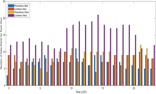
The relatively large standard errors for some of these results are largely due to the scarcity of data. For the pre-lockdown period, 9.4% of hours were lost due to instrument failure, 0.6% of data were removed by EddyPro, 7.4% of data were removed for low turbulence, and 5.7% of data were removed due to an extreme CO₂ flux, latent heat flux, or sensible heat flux value. For the lockdown period, 0.2% of hours were removed by EddyPro, 12.7% were removed for low turbulence, and 2.6% were removed for an extreme value. Following filtering and analysis, the east sector CO₂ff pre-lockdown period had an average of N = 6.6 measurements taken for each hour of the day, and the lockdown period had an average of N = 8.0 measurements taken for each hour. In the west sector, pre-lockdown had an average of N = 8.6 measurements and lockdown had an average of N = 14.8 measurements. The hourly distribution of these data points can be seen in Figure 4. The error bars in Figure 3 represent standard error, so they are based on the number of data points each hour. In Figure 3(g) (east sector), the average hourly CO₂ff emission uncertainty for pre-lockdown is ± 45.0% and lockdown is ± 69.5%. In Figure 3(c) (west sector), the average hourly CO₂ff emission uncertainty for pre-lockdown is ± 98.7% and lockdown is ± 141.3%. Uncertainties in the daily mean fluxes are considerably smaller, making it easier to detect significant emissions changes (Table 2) even for this limited duration, two wind-sector data set.

Figure 4. Bar graph representing the number of datapoints used to calculate the average emissions for each hour of the weekday in each period (pre-lockdown and lockdown) and sector (east and west).

Hestia inventory model comparison with eddy covariance flux measurements

Hestia estimates also indicate a decrease in fossil fuel emissions during Indianapolis’ COVID-19 lockdown. The average daily cycles in the west sector (Figure 5(a)) and the east sector (Figure 5(b)) are noticeably shorter during the lockdown. Both sectors have rush hour peaks indicative of the influence of traffic emissions, although those of the west sector are much less pronounced (Figure 5). According to Hestia, the average CO₂ff emission to the east dropped by 12 ± 1 µmol m⁻² s⁻¹ (56 ± 7%) and to the west it dropped by 4.4 ± 0.3 µmol m⁻² s⁻¹ (63 ± 4%) (Table 3). When breaking down Hestia estimates by source, one can see that onroad and commercial sources are the most prevalent sources east of the tower and the most affected by the lockdown (Table 3). Onroad emissions in the direction of the highway dropped by 5.4 ± 0.5 µmol m⁻² s⁻¹ between pre-lockdown and lockdown, while residential dropped by 0.23 ± 0.02 µmol m⁻² s⁻¹. Residential emissions, much greater to the west, also drop during the lockdown period, likely due to increased temperatures limiting the need for home heating (Table 3). Emissions from nonroad sources such as lawnmowers, golf carts, construction equipment, etc. were low in Hestia to the east and west of US-INg (Table 2). Unlike the other sources, they increased slightly during lockdown, though not enough to offset the other sources’ reductions.

Figure 5. Daily cycles of total CO₂ emissions estimated by Hestia from (a) west sector and (b) east sector. Error bars represent standard error.

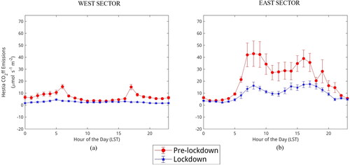
Table 3. Reductions for the major individual sources that contribute to the Hestia emissions estimate. Absolute reductions in µmol m⁻² s⁻¹, percent reduction shown in parentheses. Uncertainties represent standard error.

Emissions source	West Δ µmol CO2 m^−2 s^−1 (Δ%)	East Δ µmol CO2 m^−2 s^−1 (Δ%)
Hestia (Onroad)	0.64 ± 0.07 (41 ± 5%)	5.4 ± 0.5 (42 ± 4%)
Hestia (Commercial)	0.72 ± 0.06 (80 ± 9%)	6.9 ± 1.0 (84 ± 16%)
Hestia (Residential)	3.1 ± 0.2 (74 ± 7%)	0.23 ± 0.02 (64 ± 6%)
Hestia (Nonroad)	−0.074 ± 0.003 (−26 ± 1%)	−0.12 ± 0.03 (−21 ± 5%)

Hestia shows similar daily emissions cycles to those observed using the tower-based EC flux data, especially to the east. There is statistically significant correlation between CO₂ff average hourly emissions and Hestia emissions in the east sector for the pre-lockdown (r = 0.73, p = 4.4 × 10⁻⁵) and lockdown period (r = 0.59, p = 0.0024), although it is less significant during the lockdown period (Table 4). Correlation is not significant to the west for pre-lockdown (r = 0.29, p = 0.17) and lockdown (r = −0.10, p = 0.64), but the correlation is still higher before lockdown than during (Table 4).

Table 4. Correlations between average daily cycles from US-INg results and Hestia results. Correlation is significant if p < 0.05.

	r	p
CO2ff vs Hestia (East, pre-lockdown)	0.73	4.4 × 10^−5
CO2ff vs Hestia (East, lockdown)	0.59	0.0024
CO2ff vs Hestia (West, pre-lockdown)	0.29	0.17
CO2ff vs Hestia (West, lockdown)	−0.10	0.64

The reductions shown in Table 3 for Hestia are remarkably similar, easily within the standard error of the measurements, for CO₂ff emissions from the east sector. Hestia suggests this reduction is due to roughly equivalent reductions in onroad and commercial sector emissions (Table 3). Hestia predicts a larger magnitude of CO₂ff emission reduction from the western sector than is suggested by the disaggregated EC flux measurements, but the magnitude of the difference is small, and the percentage reductions in both products are indistinguishable given the uncertainty in the flux measurements (Table 3). Overall, both methods of quantifying CO₂ff emissions tell a similar story of large emissions reductions during the COVID-19 lockdown, similar reduction amounts and greater magnitude reductions in the east sector.

Evaluation of potential fluctuations in R_CO

The vertical differences in CO and CO₂ do not suggest significant local differences from the city-wide values in R_CO, and do not show any clear changes from the pre-lockdown to the lockdown period. The R_CO values from the eastern sector show no significant change over time. For pre-lockdown the median R_CO is 7.4 ppb ppm⁻¹ and the median R_CO uncertainty (σ) is 1.5 ppb ppm⁻¹. For lockdown, the median R_CO is 7.1 ppb ppm⁻¹ and the median uncertainty (σ) is 1.5 ppb ppm⁻¹. Neither value differs significantly from the 8 ppb ppm⁻¹ value for the whole city [21]. Breaking the data into day and night conditions yields an unusual change, but the significance is questionable. During the pre-lockdown period, daylight R_CO had a median value of 7.6 ppb ppm⁻¹ and a median σ of 2.4 ppb ppm⁻¹ while nighttime R_CO had a median value of 7.5 ppb ppm⁻¹ and a median σ of 2.0 ppb ppm⁻¹. During the lockdown period, median daylight R_CO was 6.3 ppb ppm⁻¹ (median σ = 2.4 ppb ppm⁻¹), and median nighttime R_CO was 8.4 ppb ppm⁻¹ (median σ = 2.1 ppb ppm⁻¹). So, during the pre-lockdown period, R_CO did not vary much between night and day but during the lockdown period, there was more differentiation between night and day R_CO. This day-to-night change is the opposite of what might be expected due to increased biological activity and may be an artifact from limited sampling.

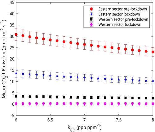
The CO₂ff flux results of the east and west sectors also did not change significantly when using different values of R_CO in the disaggregation calculation. R_CO only influences the flux partitioning, not the variability in time, so the correlation with Hestia is not influenced by the R_CO values used. Percent reductions between pre-lockdown and lockdown average emissions did not change for R_CO values between 6 ppb ppm⁻¹ and 8 ppb ppm⁻¹, so long as the pre-lockdown and lockdown periods used the same R_CO value. The magnitude of estimated CO₂ff emissions does change with the R_CO value (Figure 6). Changing the R_CO value of one period but not the other does affect the percent reduction. Fixing R_CO at 6.0 ppb ppm⁻¹ for pre-lockdown and cycling from 6.0 to 8.0 ppb ppm⁻¹ for lockdown the percent reduction in CO₂ff emissions to the east changed from 51.5% to 63.7%.

Figure 6. Mean CO₂ff emissions (excluding weekends) for each period in each sector vs. R_CO. Error bars represent standard error.

Discussion

Source disaggregated EC flux measurements indicate a drop in fossil fuel emissions during the COVID-19 lockdown like those estimated by the Hestia inventory model. The reduction was greater in the east sector than the west sector according to the EC flux measurements and Hestia, which is unsurprising given the location of the highway to the east and a suburban forest and neighborhood to the west. The Hestia sector breakdown in Table 3 shows that the reduction in the East sector was mostly due to reductions in traffic and commercial emissions. Since Google mobility data show reductions in mobility during the lockdown period, Hestia’s traffic sector uses local traffic data for sub-annual scaling, and these reductions coincide with high Oxford Stringency ratings, likely, this reduction in emissions to the East observed by Hestia and US-INg is due to the COVID-19 lockdown [1,38]. Sub-annual commercial emission patterns in Hestia are scaled using temperature data, so changes in commercial emissions between pre-lockdown and lockdown are not due to lockdown measures. However, it is possible that commercial emissions did not change appreciably due to COVID-19 since commercial buildings likely still used climate control, electricity, etc., during the lockdown. If the Hestia sectoral breakdown is accurate, roughly half the reduction in emissions during lockdown was due to COVID-19 lockdown effects on human activity.

According to temperature data from the National Weather Service collected at the Indianapolis International Airport (about 6 km from US-INg), temperature patterns in 2020 were close to normal [47]. This is important to remember when considering emissions sources such as the commercial sector that depend on temperature data. The residential sector of Hestia, whose sub-annual patterns are also dependent on temperature data, reported reductions in emissions in both directions, especially the west (Table 3). Since the Hestia sector analysis shows that the residential sector’s reductions were dominant to the West, it is likely that reductions observed by US-INg and Hestia in CO₂ff emissions are attributable to rising springtime temperatures as heating requirements are reduced.

Hestia and EC analyses of the percentage reduction in CO₂ff emissions match from both wind directions within the levels of uncertainty estimated by the EC fluxes (Table 3). The magnitude of CO₂ff emissions reductions estimated by EC fluxes are lower from the west than in Hestia (Table 3). This could be the result of issues with the EC fluxes, Hestia, or both, but the emissions reductions magnitudes are small in both products. Google mobility data reported an increase in users going to their residence during the lockdown, which one might expect to result in an increase in residential emissions [1]. This change would not be apparent in Hestia’s estimates, but it is possible that it was measured by US-INg which could explain why US-INg reports a less severe drop in CO₂ff emissions than Hestia (Table 3). The magnitude of emission reductions from the east agrees remarkably well (Table 3).

Our EC flux analyses, while limited by sampling time (about six weeks from each period), divided among two different environments (highway-dominated eastern and suburban/forested western sectors), and complicated by fossil/biogenic CO₂ flux disaggregation, are still able to identify important changes in emissions from each of the wind sectors. The pre-lockdown correlations between the daily cycle of CO₂ff emissions from Hestia and EC flux results demonstrates the ability of the flux disaggregation method even when limited by the relatively small number of hours with winds from the eastern sector, and the need to segregate modest CO₂ff emissions from the biological fluxes from the western sector. The loss of correlation during the lockdown is reasonable since the amplitude of the daily cycle of CO₂ff emissions is greatly suppressed. Lower correlations in the west sector are understandable for the same reason.

The EC analyses for this case are small enough to detect the changes in CO₂ff emissions caused by the pandemic. The noise levels, however, are significant (Figure 3) due to the limited number of data points available when limiting the sampling time to only 6 weeks and breaking the data down by wind direction. The fluxes from the west are further limited by some uncertainty in R_CO and the need for significant flux disaggregation, as opposed to the eastern sector which is dominated by fossil emissions. The uncertainties in our hourly (Figure 3) and period-average (Table 2) EC fluxes provide insight into our overall ability to quantify emissions changes using source-disaggregated EC methods.

There were other results that suggested this research was approaching its limits, such as the large hourly CO₂bio results east of US-INg (Figure 3(h)). Since the hourly averages were fluctuating around 0 and had no recognizable biological pattern, it seems likely that these results are from variation in the CO₂ff estimates. The negative hourly averages occasionally present in the CO and CO₂ff daily cycles (Figure 3(b, c, f, and g)) are also unrealistic and probably a result of error in the disaggregation analysis, introduced by negative eddy diffusivity (K) values. Negative K values do not make physical sense but filtering out negative K values resulting from instrumental noise would mean leaving positive K values from instrumental noise in, thus biassing the results. The negative hourly average emissions in the CO₂ff results are always smaller than the estimated uncertainty, so they are not significantly different from 0 and should not be over-interpreted.

The findings of this study agree with those from other studies that COVID-19 lockdown measures lead to a decrease in anthropogenic CO₂ emissions [2–6,9,10,18,19,48,49]. This study and others show that EC is particularly useful for looking at how specific regions and emissions sectors were affected by COVID-19 lockdowns. US-INg and Hestia results indicated that emissions reductions varied depending on the region and its associated emissions sectors. The EC study in Vienna, Austria only found reductions in 2020 compared to previous years in the mean CO₂ flux consistently greater than the standard error to the northwest of the tower where it is more populous and urbanized [18]. To the southeast of the EC tower, the city was less urbanized and had a non-significant emissions reduction in 2020 compared to 2018 and 2019 [18]. This is reminiscent of the current result that the more urbanized east sector showed larger reductions in magnitude. (Figure 3). Our study also suggested that the less urbanized area was less sensitive to COVID-19 restrictions, since Hestia sector analysis showed that emissions changes to the west due to COVID-19 restrictions may be negligible compared to seasonal changes.

Differences in space and time in R_CO greater than uncertainty were not detected using the vertical differences in CO and CO₂ mole fractions. This is surprising given the large changes in emissions that occurred during the lockdown. The uncertainty in derived R_CO, however, was large. In addition, both traffic (a high R_CO source) and commercial (low R_CO source) CO₂ff emissions decreased based on Hestia’s partitioning, so R_CO of the mixture of sources that are detected in the atmosphere may have remained approximately constant.

Conclusions

Three months of source- and sector-disaggregated EC flux measurements from a single tower clearly captured a rapid change in CO₂, CO, and CO₂ff emissions caused by the COVID-19 lockdown in two adjacent but contrasting neighborhoods of Indianapolis. Hestia, a research-grade inventory model for CO₂ff emissions, predicted a similar reduction in emissions. The close agreement between EC estimates of CO₂ff emissions and Hestia, and the relatively small uncertainty in the EC-based estimate suggests high confidence in both estimates of the drop in CO₂ff emissions that resulted during the COVID-19 lockdown in a highway-dominated neighborhood of Indianapolis. Emissions reductions from the western, suburban region, were much smaller in magnitude and more uncertain as a fraction of the total drop, but both Hestia and the disaggregated EC results showed a small but significant drop in CO₂ff emissions from that neighborhood. Emissions sector analysis of Hestia suggests that reductions to the east are likely in large part due to mobility restrictions during the COVID-19 pandemic, but reductions to the west may be a result of typical seasonal weather patterns reducing the need for home climate control.

Future research in this vein would benefit from a more precise method of determining R_CO at the scales measured by EC flux systems. Disaggregation of fossil and biological flux is critical to analyzing spatial and temporal patterns of CO₂ff emissions in urban settings, and CO:CO₂ff ratios are a powerful tool for disaggregation. This ability to disaggregate will also support studies of urban ecosystem.

An increasing body of evidence is showing that EC measurement systems enable precise monitoring of urban greenhouse gas emissions. These measurement systems should be developed in parallel with the development of urban emissions models whose spatial and temporal resolutions are well-matched to the resolution of EC flux measurements. EC flux measurements can complement both research-grade emission models and operational inventories created by municipalities for emissions reporting. The combination of high-resolution measurements and models will enable an increasingly precise and accurate understanding of urban metabolism, and improved ability to monitor and predict the impacts of greenhouse gas emissions mitigation measures.

Acknowledgments

We thank the program directors Dr. Raymond Najjar and Dr. Gregory Jenkins for their continued support of the Penn State Climate Science REU program. The INFLUX and NIST teams provided invaluable data, help, and insights into COVID-19’s effects on urban emissions. We thank Ms. Krittika Shahani and Dr. Alex Zhang for their help with computing, data acquisition, and analysis.

Disclosure statement

No potential conflict of interest was reported by the author(s).

Data availability statement

The eddy-covariance data used for this research are available at https://doi.org/10.26208/2YQZ-5S85. The CO and CO₂ mole fraction measurements are available at https://doi.org/10.18113/D37G6P. The Hestia model data are available at https://doi.org/10.26208/H62J-4004.

Additional information

Funding

This research was conducted as part of the Climate Science Experience for Undergraduates program and funded by the National Science Foundation under grant number AGS-1852428. INFLUX is funded by the National Institute of Standards and Technology (Penn State, Project # 70NANB19H128 and # 70NANB23H188; Northern Arizona University, Project # 70NANB19H129). This work was also supported by NOAA’s Atmospheric Carbon, Chemistry, Composition and Climate (AC4) program via Grant NA21OAR4310227.

References

- COVID-19 Community Mobility Reports [Internet]. Googleplex: Google LLC; 2024 [cited 2024 Jan 2]. Available from: https://www.google.com/covid19/mobility/
- Loo BPY, Huang Z. Spatio-temporal variations of traffic congestion under work from home (WFH) arrangements: lessons learned from COVID-19. Cities. 2022;124:103610. doi: 10.1016/j.cities.2022.103610.
- Tian X, An C, Chen Z, et al. Assessing the impact of COVID-19 pandemic on urban transportation and air quality in Canada. Sci Total Environ. 2021;765:144270. doi: 10.1016/j.scitotenv.2020.144270.
- Le Quéré C, Jackson RB, Jones MW, et al. Temporary reduction in daily global CO2 emissions during the COVID-19 forced confinement. Nat Clim Chang. 2020;10(7):647–653. doi: 10.1038/s41558-020-0797-x.
- Schulte-Fischedick M, Shan Y, Hubacek K. Implications of COVID-19 lockdowns on surface passenger mobility and related CO2 emission changes in Europe. Appl Energy. 2021;300:117396. doi: 10.1016/j.apenergy.2021.117396.
- Zhang X, Li Z, Wang J. Impact of COVID-19 pandemic on energy consumption and carbon dioxide emissions in China’s transportation sector. Case Stud Therm Eng. 2021;26:101091. doi: 10.1016/j.csite.2021.101091.
- Toro AR, Catalán F, Urdanivia FR, et al. Air pollution and COVID-19 lockdown in a large South American city: Santiago Metropolitan Area, Chile. Urban Clim. 2021;36:100803. doi: 10.1016/j.uclim.2021.100803.
- Collivignarelli MC, Abbà A, Bertanza G, et al. Lockdown for CoViD-2019 in Milan: what are the effects on air quality? Sci Total Environ. 2020;732:139280. doi: 10.1016/j.scitotenv.2020.139280.
- Weir B, Crisp D, O'Dell CW, et al. Regional impacts of COVID-19 on carbon dioxide detected worldwide from space. Sci Adv. 2021;7(45):eabf9415. doi: 10.1126/sciadv.abf9415.
- Monteiro V, Miles NL, Richardson SJ, et al. The impact of the COVID-19 lockdown on greenhouse gases: a multi-city analysis of in situ atmospheric observations. Environ Res Commun. 2022;4(4):041004. doi: 10.1088/2515-7620/ac66cb.
- Moncrieff J, Valentini R, Greco S, et al. Trace gas exchange over terrestrial ecosystems: methods and perspectives in micrometeorology. J Exp Bot. 1997;48(5):1133–1142. doi: 10.1093/jxb/48.5.1133.
- Velasco E, Roth M. Cities as net sources of CO2: review of atmospheric CO2 exchange in urban environments measured by Eddy Covariance technique. Geogr Compass. 2010;4(9):1238–1259. doi: 10.111/j.1749-8198.2010.00384.x.
- Crawford B, Christen A, McKendry I. Diurnal course of carbon dioxide mixing ratios in the urban boundary layer in response to surface emissions. J Appl Meteor Climatol. 2016;55(3):507–529. doi: 10.1175/JAMC-D-15-0060.1.
- Matese A, Gioli B, Vaccari FP, et al. Carbon dioxide emissions of the city center of Firenze, Italy: measurement, evaluation, and source partitioning. J Appl Meteor Climatol. 2009;48(9):1940–1947. doi: 10.1175/2009JAMC1945.1.
- Helfter C, Tremper AH, Halios CH, et al. Spatial and temporal variability of urban fluxes of methane, carbon monoxide, and carbon dioxide above London, UK. Atmos Chem Phys. 2016;16(16):10543–10557. doi: 10.5194/acp-16-10543-2016.
- Ishidoya S, Sugawara H, Terao Y, et al. O2: CO2 exchange ratio for net turbulent flux observed in an urban area of Tokyo, Japan, and its application to an evaluation of anthropogenic CO2 emissions. Atmos Chem Phys. 2020;20(9):5293–5308. doi: 10.5194/acp-20-5293-2020.
- Sugawara H, Ishidoya S, Terao Y, et al. Anthropogenic CO2 emissions changes in an urban area of Tokyo, Japan, due to the COVID-19 pandemic: a case study during the state of emergency in April-May 2020. Geophys Res Lett. 2021;48(15). doi: 10.1029/2021GL092600.
- Matthews B, Schume H. Tall tower eddy covariance measurements of CO2 fluxes in Vienna, Austria. Atmos Environ. 2022;274:118941. doi: 10.1016/j.atmosenv.2022.118941.
- Nicolini G, Antoniella G, Carotenuto F, et al. Direct observations of CO2 emissions reductions due to COVID-19 lockdown across European urban districts. Sci Total Environ. 2022;830. doi: 10.1016/j.scitotenv.2022.154662.
- Wu K, Davis KJ, Miles NL, et al. Source decomposition of eddy-covariance CO2 flux measurements for evaluating a high-resolution urban CO2 emissions inventory. Environ Res Lett. 2022;17(7):074035. doi: 10.1088/1748-9326/ac7c29.
- Turnbull JC, Sweeney C, Karion A, et al. Toward quantification and source sector identification of fossil fuel CO2 emissions from an urban area: results from the INFLUX experiment. JGR Atmosph. 2014;120(1):292–312. doi: 10.1002/2014JD022555.
- Vogel, E, Richardson, SJ, Miles, NL, Davis, KJ, INFLUX suburban carbon dioxide flux tower data. Data set. Pennsylvania State University Data Commons, University Park, Pennsylvania, USA.; 2023. Available from: http://datacommons.psu.edu. doi: 10.26208/2YQZ-5S85.
- Miles NL, Richardson SJ, Davis KJ, et al. In-situ tower atmospheric measurements of carbon dioxide, methane and carbon monoxide mole fraction for the Indianapolis Flux (INFLUX) project, Indianapolis, IN, USA. Data set. The Pennsylvania State University Data Commons, University Park, Pennsylvania, USA; 2017. Available from: http://datacommons.psu.edu. doi: 10.18113/D37G6P.
- Davis KJ, Deng A, Lauvaux T, et al. The Indianapolis Flux Experiment (INFLUX): a test-bed for developing urban greenhouse gas emission measurements. Elem Sci Anth. 2017;5(21). doi: 10.1525/elementa.188.
- Heimburger AMF, Harvey RM, Shepson PB, et al. Assessing the optimized precision of the aircraft mass balance method for measurement of urban greenhouse gas emission rates through averaging. Elem Sci Anth. 2017;5(26). doi: 10.1525/elementa.134.
- Lauvaux T, Gurney KR, Miles NL, et al. Policy-relevant assessment of urban CO2 emissions. Environ Sci Technol. 2020;54(16):10237–10245. doi: 10.1021/acs.est.0c00343.
- Richardson SJ, Miles NL, Davis KJ, et al. Tower measurement network of in-situ CO2, CH4, and CO in support of the Indianapolis FLUX (INFLUX) experiment. Elem Sci Anth. 2017;5:59. doi: 10.1525/elementa.140.
- U.S. Geological Survey. USGS One-Meter x56y441 in Central Marion Co 2016; 2020.
- LI-COR, Inc. EddyPro® version 7.0 help and user’s guide. Lincoln, NE: LI-COR, Inc; 2021.
- Foken T, Nappo CJ. Micrometeorology. New York, NY: Springer; 2008.
- Lee X, Massman W, Law B. A perspective on thirty years of the Webb. Boundary Layer Meteorol. 2011;139(1):37–59. doi: 10.1007/s10546-010-9575-z.
- Wilczak JM, Oncley SP, Stage SA. Sonic anemometer tilt correction algorithms. Boundary Layer Meteorol. 2001;99(1):127–150. doi: 10.1023/A:1018966204465.
- Lee X, Massman W, Law B.Handbook of micrometeorology. In: Lee X, Massman X, Law B, editor. Handbook of micrometeorology. Vol. 29. Netherlands: Springer; 2005. doi: 10.1007-4020-2265-4.
- Webb EK, Pearman GI, Leuning R. Correction of flux measurements for density effects due to heat and water vapour transfer. Quart J Royal Meteoro Soc. 1980;106(447):85–100. doi: 10.1002/qj.49710644707.
- Vickers D, Mahrt L. Quality control and flux sampling problems for tower and aircraft data. J Atmos Oceanic Technol. 1997;14(3):512–526. doi: 10.1175/1520-0426(1997)014<0512:QCAFSP>2.0.CO;2.
- Yi C, Davis KJ, Bakwin PS, et al. Influence of advection on measurements of the net ecosystem-atmosphere exchange of CO2 from a very tall tower. J Geophys Res. 2000;105(D8):9991–9999. doi: 10.1029/2000JD900080.
- King C. Our year of COVID: Key dates in Indiana’s fight against the coronavirus. Indianapolis Star; 2021, March 18 [cited 2024 Jan 2] Available from: https://www.indystar.com/in-depth/news/2021/03/18/indiana-covid-timeline-key-dates-states-fight-vs-pandemic/6813412002/
- Hale T, Angrist N, Goldszmidt R, et al. A global panel database of pandemic policies (Oxford COVID-19 Government Response Tracker). Nat Hum Behav. 2021;5(4):529–538. doi: 10.1038/s41562-021-01079-8.
- Browaeys J. Linear fit with both uncertainties in x and in y. MATLAB Central File Exchange; 2022. [updated 2017 Oct 25; cited 2022 June 23]. Available from: https://www.mathworks.com/matlabcentral/fileexchange/45711-linear-fit-with-both-uncertainties-in-x-and-in-y
- Gurney KR, Razlivanov I, Song Y, et al. Quantification of fossil fuel CO2 emissions on the building/street scale for a large city. Environ Sci Technol. 2012;46(21):12194–12202. doi: 10.1021/es3011282.
- Gurney KR, Liang J, O’Keeffe D, et al. Comparison of global downscaled versus bottom-up fossil fuel CO2 emissions at the urban scale in four US urban areas. J Geophys Res D Atmos. 2018;124(5):2823–2840. doi: 10.1029/2018JD028859.
- Roest G, Gurney KR, Vogel E, et al. Hestia Fossil Fuel Carbon Dioxide (FFCO2) Data Product – Indianapolis, Version 3.2, 20m Grid at Flux Towers. State College, PA: Penn State Data Commons; 2023. doi: 10.26208/H62J-4004.
- Kljun N, Calanca P, Rotach MW, et al. A simple two-dimensional parameterisation for Flux Footprint Prediction (FFP). Geosci Model Dev. 2015;8(11):3695–3713. doi: 10.5194/gmd-8-3695-2015.
- Hersbach H, Bell B, Berrisford P, et al. ERA5 hourly data on single levels from 1940 to present. Copernicus Climate Change Service (C3S) Climate Data Store (CDS); 2023. doi: 10.24381/cds.adbb2d47.
- Tennekes H. The logarithmic wind profile. J Atmos Sci. 1973;30(2):234–238. doi: 10.1175/1520-0469(1973)030<0234:TLWP>2.0.CO;2.
- Mead R, Nelder JA. A simplex method for function minimization. Comput. J. 1965;7(4):308–313. doi: 10.1093/comjnl/7.4.308.
- Iowa Environmental Mesonet. [Internet]. Iowa State University. [cited 2024 February 6]. Available from: https://mesonet.agron.iastate.edu/request/download.phtml?network=IN_ASOS.
- Velasco E. Impact of Singapore’s COVID-19 confinement on atmospheric CO2 fluxes at neighborhood scale. Urban Clim. 2021;37:100822. doi: 10.1016/j.uclim.2021.100822.
- Yadav V, Ghosh S, Mueller K, et al. The impact of COVID-19 on CO2 emissions in the Los Angeles and Washington DC/Baltimore metropolitan areas. Geophys Res Lett. 2021;48(11):e2021GL092744. doi: 10.1029/2021GL092744.
- U.S. Census Bureau. 2020 Census Demographic Data Map Viewer; 2020. Available from: https://maps.geo.census.gov/ddmv/map.html
- Stewart ID, Oke TR. Local climate zones for urban temperature studies. Bull Amer Metor Soc. 2012;93(12):1879–1900. doi: 10.1175/BAMS-D-11-00019.1.
- Dewitz J, U.S. Geological Survey. National Land Cover Database (NLCD) 2019 products (ver. 2.0, June 2021). U.S. Geological Survey Data Release; 2021. Reston, Virginia. doi: 10.5066/P9KZCM54.