Distributed control for bi-connectivity of multi-robot network

ABSTRACT

This paper approaches a bi-connectivity preservation problem for networked multi-robot systems in a distributed control fashion. Since a bi-connected network topology is robust against single node removal, networked multi-robot systems are required to preserve bi-connectedness in cases robots may fail. By employing a perturbed graph Laplacian to find if the network is disconnected after a node is removed, we analyse a sufficient condition that the network is bi-connected. Then we design a distributed control law to preserve the bi-connectedness from the sufficient condition. Moreover, considering cases a robot fails, we propose a control law to let a uni-connected network be bi-connected forcibly. A condition to restore the bi-connectedness by the proposed control is theoretically proved. The effectiveness of the proposed control laws is demonstrated by numerical simulations.

KEYWORDS:

• Multi-robot systems
• network connectivity
• distributed control
• bi-connectivity
• connectivity control

1. Introduction

Multi-robot systems are the systems in which each robot individually makes each decision by communicating with each other. One of the control strategies for such multi-robot systems is a coverage [1] of which the control objective is to cover a given area by the range of sensors equipped by the robots. The coverage control methods are applied for target searching and consisting a mobile ad-hoc network.

To achieve the team objectives through communication or information exchange, it is important that a network modelling the communication topology is connected. The task accomplishment will be hard once the connectedness is lost since the network topology will be divided into two or more components. For this challenge, some autonomous distributed control laws to preserve the connectedness have been proposed [2,3]. Since it is known that the connectedness is equivalent to the second smallest eigenvalue of the graph Laplacian matrix is positive, a lot of the control laws for the connectedness preservation employ the gradient of the second smallest eigenvalue to decide the direction of the robot motion. The second smallest eigenvalue of the graph Laplacian is called algebraic connectivity.

The network connectedness will be violated by the failure of the robots. Bi-connectedness is required to preserve the network connected against a single robot failure and therefore distributed control laws to preserve bi-connectedness have been proposed [4,5]. The work [4] clarified the theoretical fact that the network is bi-connected if and only if the third smallest eigenvalue of the modified Laplacian matrix is positive, and the control method to preserve the third smallest eigenvalue is proposed. However, calculating only the third smallest eigenvalue in a distributed fashion is difficult. Calculating all the eigenvalues is assumed to get the third one, but it requires a lot of computation and communication costs. Apart from connectivity control using the Laplacian eigenvalue, a control algorithm with vertex connectivity of a subgraph is proposed in [5] for connectivity maintenance. A cost function of the vertex connectivity which is calculated in a distributed fashion is designed in that work, but the control algorithm using the cost function does not theoretically guarantee the vertex connectivity under the existence of the task input.

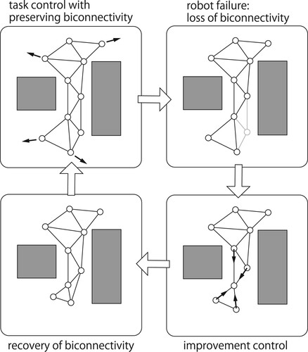
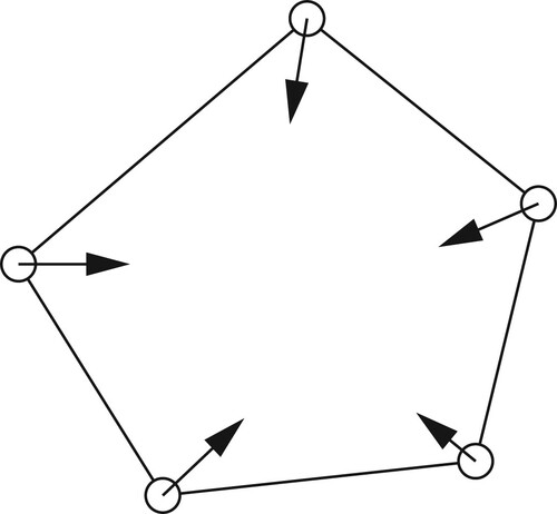
We have proposed a hybrid control method for the bi-connectivity of the multi-robot network using the second smallest eigenvalue of the perturbed Laplacian matrix in the study [6]. Since the second smallest eigenvalue of the Laplacian is efficiently computed by a distributed algorithm [7] unlike the third smallest eigenvalue, overall computation of our control method is accomplished in a distributed fashion. The proposed hybrid control switches two control modes: an improvement control and a preservation control for the bi-connectedness (see Figure 1). The improvement control works when the bi-connectedness is violated by a robot failure, and the preservation control enables the multi-robot system to accomplish a team task with preserving the bi-connectedness. The theoretical correctness of the control laws are proved using results of our previous studies [8,9] where we analysed that the second smallest eigenvalue of a perturbed Laplacian is related to the connected components of the network after single robot failure. Additionally, we had claimed that our improvement control method may not resume the bi-connectedness under some conditions.

Figure 1. Preservation and improvement of network bi-connectedness.

This paper proposes a refined version of the control method for the multi-robot network bi-connectedness. We try to overcome the bi-connectivity improvement difficulty claimed in the study [6] by stopping the preservation control temporarily. The detailed scheme of the control method and results of the numerical simulation are presented here.

The rest of this paper is organized as follows: Section 2 defines a networked multi-robot system we discuss in this work and formulate a bi-connectivity control problem that is designed to robustify the multi-robot network topology against robotic failures. We propose control methods to solve the bi-connectivity problem in Section 3. Perturbed algebraic connectivity is introduced from our previous studies, and control laws are constructed by employing perturbed algebraic connectivity. In Section 4, results of numerical simulations are demonstrated to represent the effectiveness of the proposed method. Section 5 concludes this paper.

2. Problem formulation

In this section, we define a multi-robot system we consider in this study, and the control problem we try to solve. We assume the multi-robot system consisting of $N\ge 3$ autonomous mobile robots, and define the index set of the robots by $\mathcal{V}=\{1,2,\dots ,N\}$.

The motion dynamics of each robot is formulated as (1) ${\dot{x}}_i\left(t\right)=k_i^{\mathrm{b}\mathrm{c}}{u}_i^{\mathrm{b}\mathrm{c}}\left(t\right)+k_i^{\mathrm{t}\mathrm{a}\mathrm{s}\mathrm{k}}{u}_i^{\mathrm{t}\mathrm{a}\mathrm{s}\mathrm{k}}\left(t\right),$(1) where $t\ge 0$ denotes continuous time, $x_i\in {\mathbf{R}}^d$ denotes position of robot $i\in \mathcal{V}$, $u_i^{\mathrm{b}\mathrm{c}}\in {\mathbf{R}}^d$ denotes a control input of the improvement/preservation for the bi-connectedness, $u_i^{\mathrm{t}\mathrm{a}\mathrm{s}\mathrm{k}}\in {\mathbf{R}}^d$ denotes a task control input such like coverage or target searching. $k_i^{\mathrm{b}\mathrm{c}}$ and $k_i^{\mathrm{t}\mathrm{a}\mathrm{s}\mathrm{k}}$ are control gains, and $d\in \{2,3\}$ is a dimension of the configuration space. We assume the task control $u_i^{\mathrm{t}\mathrm{a}\mathrm{s}\mathrm{k}}$ is repulsive from neighbour robots as a coverage control, so that the task control act as a disturbance of bi-connectedness.

Two robots i and j have a communication link when the distance ${\mathrm{d}\mathrm{i}\mathrm{s}\mathrm{t}}_{ij}\left(t\right)=\Vert x_i\left(t\right)-x_j\left(t\right)\Vert$ is less than the communication radius R and there are no obstacles on the line segment from the point $x_i$ to the point $x_j$ (hereafter we represent this line segment as $\mathrm{s}\mathrm{e}\mathrm{g}(x_i,x_j)$). The network topology $\mathcal{G}\left(t\right)=(\mathcal{V},\mathcal{E}(t\left)\right)$ is represented by the weighted adjacency matrix $A\left(t\right)$, such that $\mathcal{E}\left(t\right)=\left\{\right(i,j)\in \mathcal{V}\times \mathcal{V}|a_{ij}\left(t\right)>0\}$ where $a_{ij}$ denotes the ijth entry of the adjacency matrix A. We employ definitions of the ijth entry $a_{ij}$ from a previous study [10], as (2) $a_{ij}={\gamma }^a\left({\mathrm{d}\mathrm{i}\mathrm{s}\mathrm{t}}_{ij}\right)\prod _{k\in {\mathcal{O}}_{ij}}{\gamma }^b\left({\mathrm{d}\mathrm{i}\mathrm{s}\mathrm{t}}_{ijk}\right),$(2) where ${\mathrm{d}\mathrm{i}\mathrm{s}\mathrm{t}}_{ijk}$ denotes the distance from the obstacle $k\in \mathcal{O}$ to the line segment $\mathrm{s}\mathrm{e}\mathrm{g}(x_i,x_j)$. ${\mathcal{O}}_{ij}$ denotes the indexes set of the obstacles to which the distance from the segment $\mathrm{s}\mathrm{e}\mathrm{g}(x_i,x_j)$ are less than $d_{max}$, that is, ${\mathcal{O}}_{ij}=\{k\in \mathcal{O}|{\mathrm{d}\mathrm{i}\mathrm{s}\mathrm{t}}_{ijk}<d_{max}\}$. The functions ${\gamma }^a\left({\mathrm{d}\mathrm{i}\mathrm{s}\mathrm{t}}_{ij}\right)$ and ${\gamma }^b\left({\mathrm{d}\mathrm{i}\mathrm{s}\mathrm{t}}_{ijk}\right)$ are defined by (3) ${\gamma }^a\left({\mathrm{d}\mathrm{i}\mathrm{s}\mathrm{t}}_{ij}\right)=1-{(1+\exp (-{\alpha }_a(\frac{{\mathrm{d}\mathrm{i}\mathrm{s}\mathrm{t}}_{ij}}{R}-{\text{β}}_a)))}^{-1},$(3) if ${\mathrm{d}\mathrm{i}\mathrm{s}\mathrm{t}}_{ij}<R$, otherwise ${\gamma }^a\left({\mathrm{d}\mathrm{i}\mathrm{s}\mathrm{t}}_{ij}\right)=0$, and (4) ${\gamma }^b\left({\mathrm{d}\mathrm{i}\mathrm{s}\mathrm{t}}_{ijk}\right)={(1+\exp (-{\alpha }_b(\frac{{\mathrm{d}\mathrm{i}\mathrm{s}\mathrm{t}}_{ijk}}{d_{max}}-{\text{β}}_b)))}^{-1},$(4) if ${\mathrm{d}\mathrm{i}\mathrm{s}\mathrm{t}}_{ijk}<d_{max}$, otherwise ${\gamma }^b\left({\mathrm{d}\mathrm{i}\mathrm{s}\mathrm{t}}_{ijk}\right)=1$, where ${\alpha }_a,{\text{β}}_a,{\alpha }_b,{\text{β}}_b>0$ denote positive coefficients. The value ${\gamma }^a$ reflects the proximity between the robots compared to the communication radius R, and the value ${\gamma }^b$ reflects the farness from the obstacle which impedes the line-of-sight between the robot. From the definition Equation (2(2) $a_{ij}={\gamma }^a\left({\mathrm{d}\mathrm{i}\mathrm{s}\mathrm{t}}_{ij}\right)\prod _{k\in {\mathcal{O}}_{ij}}{\gamma }^b\left({\mathrm{d}\mathrm{i}\mathrm{s}\mathrm{t}}_{ijk}\right),$(2) ), the element $a_{ij}$ gets closet to 1 only when the distance ${\mathrm{d}\mathrm{i}\mathrm{s}\mathrm{t}}_{ij}$ is sufficiently small and the distances ${\mathrm{d}\mathrm{i}\mathrm{s}\mathrm{t}}_{ijk}$ 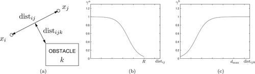are sufficiently large. Figure 2 shows an example of Equations (2(2) $a_{ij}={\gamma }^a\left({\mathrm{d}\mathrm{i}\mathrm{s}\mathrm{t}}_{ij}\right)\prod _{k\in {\mathcal{O}}_{ij}}{\gamma }^b\left({\mathrm{d}\mathrm{i}\mathrm{s}\mathrm{t}}_{ijk}\right),$(2) )–(4(4) ${\gamma }^b\left({\mathrm{d}\mathrm{i}\mathrm{s}\mathrm{t}}_{ijk}\right)={(1+\exp (-{\alpha }_b(\frac{{\mathrm{d}\mathrm{i}\mathrm{s}\mathrm{t}}_{ijk}}{d_{max}}-{\text{β}}_b)))}^{-1},$(4) ) if ${\alpha }_a={\alpha }_b=10$, ${\text{β}}_a=0.7$, and ${\text{β}}_b=0.3$. By ensuring a line of sight between two robots using the link weight function Equation (2(2) $a_{ij}={\gamma }^a\left({\mathrm{d}\mathrm{i}\mathrm{s}\mathrm{t}}_{ij}\right)\prod _{k\in {\mathcal{O}}_{ij}}{\gamma }^b\left({\mathrm{d}\mathrm{i}\mathrm{s}\mathrm{t}}_{ijk}\right),$(2) ), we try to mitigate troubles ascribed to wireless communication (e.g. interference and fading).

Figure 2. Illustrated description of link weight functions Equations (2(2) $a_{ij}={\gamma }^a\left({\mathrm{d}\mathrm{i}\mathrm{s}\mathrm{t}}_{ij}\right)\prod _{k\in {\mathcal{O}}_{ij}}{\gamma }^b\left({\mathrm{d}\mathrm{i}\mathrm{s}\mathrm{t}}_{ijk}\right),$(2) )–(4(4) ${\gamma }^b\left({\mathrm{d}\mathrm{i}\mathrm{s}\mathrm{t}}_{ijk}\right)={(1+\exp (-{\alpha }_b(\frac{{\mathrm{d}\mathrm{i}\mathrm{s}\mathrm{t}}_{ijk}}{d_{max}}-{\text{β}}_b)))}^{-1},$(4) ). (a) Definition of ${\mathrm{d}\mathrm{i}\mathrm{s}\mathrm{t}}_{ij}$ and ${\mathrm{d}\mathrm{i}\mathrm{s}\mathrm{t}}_{ijk}$. (b) ${\gamma }^a$ with respect to ${\mathrm{d}\mathrm{i}\mathrm{s}\mathrm{t}}_{ij}$ and (c) ${\gamma }^b$ with respect to ${\mathrm{d}\mathrm{i}\mathrm{s}\mathrm{t}}_{ijk}$.

Using the adjacency matrix A defined above, we define a Laplacian matrix L = D−A where D denotes the degree matrix of which the iith entry is $d_{ii}=\sum _j{a}_{ij}$. The second smallest eigenvalue ${\lambda }_2$ of the Laplacian matrix L is called the algebraic connectivity, and it is well known that the fact the graph $\mathcal{G}$ is connected if and only if ${\lambda }_2>0$.

We call the graph $\mathcal{G}\left(t\right)$ is bi-connected if a graph ${\mathcal{G}}_{-i}=(\mathcal{V}\setminus \{i\},\mathcal{E})$ stands connected for all $i\in \mathcal{V}$. When the graph ${\mathcal{G}}_{-i}$ is disconnected, the node i is called an articulation node. Clearly, we can see a bi-connected graph has no articulation node.

In this paper, we tackle two problems;

1. find a control input $u_i^{\mathrm{b}\mathrm{c}}$ and control gains $k_i^{\mathrm{b}\mathrm{c}},k_i^{\mathrm{t}\mathrm{a}\mathrm{s}\mathrm{k}}$ to preserve the graph $\mathcal{G}\left(t\right)$ is bi-connected for all time $t\ge 0$ if the initial graph $\mathcal{G}\left(0\right)$ is bi-connected,

2. and find a control input $u_i^{\mathrm{b}\mathrm{c}}$ and control gains $k_i^{\mathrm{b}\mathrm{c}},k_i^{\mathrm{t}\mathrm{a}\mathrm{s}\mathrm{k}}$ to resume the graph $\mathcal{G}\left(t\right)$ to be bi-connected in finite time $t^{\prime }>0$ if the initial graph $\mathcal{G}\left(0\right)$ is not bi-connected but uni-connected.

The first one relates to a subject before a single robot fails and the second one relates to a subject after the failure. The failure in this study means that the robot can not communicate with its neighbours whether temporarily or permanently. Later sections describe the control law to solve these problems.

3. Proposed method

We propose distributed control laws to solve the problems defined in Section 2. First, we introduce a concept of perturbed algebraic connectivity which reflects the importance of a node for the connectivity. The detailed definition and theoretical properties are written in our previous study [9]. We design the control laws using the perturbed algebraic connectivity in this study.

3.1. Perturbed algebraic connectivity

To represent the network topology after the robot i fails, using a sufficiently small positive parameter $ϵ>0$, we introduce a perturbed adjacency matrix $A^{\left(i\right)}\left(ϵ\right)$ of which the mnth element is defined by (5) $a_{pq}^{\left(i\right)}=\{\begin{array}{ll}ϵa_{pq},& \mathrm{i}\mathrm{f}p=i\mathrm{o}\mathrm{r}q=i,\\ a_{pq},& \mathrm{o}\mathrm{t}\mathrm{h}\mathrm{e}\mathrm{r}\mathrm{w}\mathrm{i}\mathrm{s}\mathrm{e},\end{array}$(5) Clearly, the perturbed adjacency matrix $A^{\left(i\right)}\left(ϵ\right)$ represents the graph topology such that the links $e_{ij}$ incident to the node i are removed from the graph $\mathcal{G}$. The perturbed Laplacian matrix $L^{\left(i\right)}\left(ϵ\right)=(D^{\left(i\right)}-A^{\left(i\right)})/d_{ii}$ and the second smallest eigenvalue ${\lambda }_2^{\left(i\right)}\left(ϵ\right)$ of the matrix $L^{\left(i\right)}\left(ϵ\right)$ are defined in a similar way, but note the perturbed Laplacian is normalized by the weighted degree $d_{ii}=\sum _j{a}_{ij}$. Assuming the graph $\mathcal{G}$ is connected, we can see ${\lambda }_2^{\left(i\right)}\left(ϵ\right)>0$ for all $ϵ>0$, and ${\lambda }_2^{\left(i\right)}\left(0\right)=0$ since the graph which all links incident to the node i is removed is disconnected. Recalling the definition of the second smallest eigenvalue ${\lambda }_2^{\left(i\right)}\left(ϵ\right)$ of the Laplacian matrix $L^{\left(i\right)}\left(ϵ\right)$, (6) ${\lambda }_2^{\left(i\right)}\left(ϵ\right)=\underset{v}{min}\frac{v^{\mathrm{\top }}{L}^{\left(i\right)}\left(ϵ\right)v}{v^{\mathrm{\top }}v},\mathrm{s}.\mathrm{t}.v^{\mathrm{\top }}\mathbf{1}=0,$(6) we can see the corresponding eigenvector $v^{\left(i\right)}\left(0\right)$ has a characteristic property; for arbitrary nodes p and q, the pth element $v_p^{\left(i\right)}$ of the eigenvector is equal to the qth element $v_q^{\left(i\right)}$ if the nodes p and q are connected in the graph ${\mathcal{G}}_{-i}$. This property is directly proved from ${\lambda }_2^{\left(i\right)}\left(0\right)=0$. From the eigenvalue definition ${\lambda }_2^{\left(i\right)}\left(ϵ\right)v^{\left(i\right)}\left(ϵ\right)=L^{\left(i\right)}\left(ϵ\right)v^{\left(i\right)}\left(ϵ\right)$, we get (7) ${\lambda }_2^{\left(i\right)}\left(ϵ\right)v_i^{\left(i\right)}\left(ϵ\right)=ϵ\sum _j\left(a_{ij}/d_{ii}\right)(v_i^{\left(i\right)}-v_j^{\left(i\right)}),$(7) where $v_j^{\left(i\right)}$ denotes the jth element of the eigenvector $v^{\left(i\right)}$.

Assuming the graph ${\mathcal{G}}_{-i}$ is composed of M>0 connected components, we discuss the gradient of the eigenvalue ${\lambda }_2^{\left(i\right)}\left(ϵ\right)$ at $ϵ=0$, defined by (8) ${\hat{\lambda }}^{\left(i\right)}=\underset{ϵ\to 0+}{lim}\frac{{\lambda }_2^{\left(i\right)}\left(ϵ\right)}{ϵ}.$(8) The node i is not an articulation when M = 1 and it is an articulation when M>1. So here we analyse the value ${\hat{\lambda }}^{\left(i\right)}$ as a function of the component number M. First, from the relations of the eigenvalue like Equation (7(7) ${\lambda }_2^{\left(i\right)}\left(ϵ\right)v_i^{\left(i\right)}\left(ϵ\right)=ϵ\sum _j\left(a_{ij}/d_{ii}\right)(v_i^{\left(i\right)}-v_j^{\left(i\right)}),$(7) ), we get equations (9a) $\begin{array}{rl}& {\hat{\lambda }}^{\left(i\right)}{v}_i=\sum _{m=1}^M{D}_m(v_i-v_{\left[m\right]}),\end{array}$(9a) (9b) $\begin{array}{rl}& {\hat{\lambda }}^{\left(i\right)}{v}_{\left[m\right]}=\frac{D_m}{C_m}(v_{\left[m\right]}-v_i),m\in \{1,\dots ,M\},\end{array}$(9b) where $D_m$ denotes the summation of the value $a_{ij}/d_{ii}$ of which node j belongs to mth connected component, and $C_m$ denotes the number of nodes in the mth component. $v_i$ denotes the ith element of the eigenvector $v^{\left(i\right)}\left(0\right)$, and $v_{\left[m\right]}$ denotes an element of the eigenvector with respect to the mth component. As we discussed in the above paragraph, the elements $v_p$ and $v_q$ are the same if both nodes p and q are in the same connected component. Note that $\sum _m{C}_m=N-1$ since it is equal to the number of nodes in the graph ${\mathcal{G}}_{-i}$, and $\sum _m{D}_m=1$ since the elements of the perturbed Laplacian matrix are normalized. From the relations Equation (9a(9a) $\begin{array}{rl}& {\hat{\lambda }}^{\left(i\right)}{v}_i=\sum _{m=1}^M{D}_m(v_i-v_{\left[m\right]}),\end{array}$(9a) ), we get an algebraic equation of the value ${\hat{\lambda }}^{\left(i\right)}$, as (10) $\sum _m\frac{D_m{C}_m}{D_m-C_m{\hat{\lambda }}^{\left(i\right)}}+1=0,$(10) with assuming $v_i\ne 0$. If $v_i=0$ and there exists a connected component m such that $v_m\ne 0$, obviously ${\hat{\lambda }}^{\left(i\right)}=D_m/C_m$ from Equation (9b(9b) $\begin{array}{rl}& {\hat{\lambda }}^{\left(i\right)}{v}_{\left[m\right]}=\frac{D_m}{C_m}(v_{\left[m\right]}-v_i),m\in \{1,\dots ,M\},\end{array}$(9b) ). The case $v_m=0$ for all $m\in \{1,\dots ,M\}$ does not occur, since $\sum _j{v}_j^{\left(i\right)}=0$ and $\Vert v^{\left(i\right)}\Vert >0$. The value ${\hat{\lambda }}^{\left(i\right)}$ is dependent on the component sizes $C_m$ and weights $D_m$, so we call it the perturbed algebraic connectivity. The perturbed algebraic connectivity ${\hat{\lambda }}^{\left(i\right)}$ is monotonically non-decreasing with respect to the link weight $a_{ij}$, since the algebraic connectivity ${\lambda }_2$ is also monotonically non-decreasing.

To analyse a condition if the node i is not an articulation one, we find the maximum value of the perturbed algebraic connectivity ${\hat{\lambda }}^{\left(i\right)}$ when the node i is an articulation.

Theorem 3.1

Corollary of [9]

Assume a graph $\mathcal{G}$ is connected, and the node i has 2 or more communication links. If the perturbed algebraic connectivity ${\hat{\lambda }}^{\left(i\right)}$ satisfies (11) ${\hat{\lambda }}^{\left(i\right)}>\frac{N}{5N-9},$(11) then the node i is not an articulation node.

Proof.

See Appendix.

From the above theorem, our objectives will be achieved by satisfying the condition (11(11) ${\hat{\lambda }}^{\left(i\right)}>\frac{N}{5N-9},$(11) ), if the perturbed algebraic connectivities are estimated in a distributed fashion. Since the algorithm proposed in the reference [7] can estimate the second smallest eigenvalue of the Laplacian matrix in a distributed fashion using, the eigenvalue ${\lambda }_2^{\left(i\right)}\left(ϵ\right)$ is also able to be estimated if $ϵ>0$. Thus, a value ${\tilde{\lambda }}^{\left(i\right)}={\lambda }_2^{\left(i\right)}/ϵ$ is employed as the approximation of the perturbed algebraic connectivity ${\hat{\lambda }}^{\left(i\right)}$ in this study. Note the approximated value is smaller than the strict value, that is, (12) $0<{\tilde{\lambda }}^{\left(i\right)}\left(ϵ\right)<{\hat{\lambda }}^{\left(i\right)},$(12) for all $ϵ>0$. This means ${\tilde{\lambda }}^{\left(i\right)}\left(ϵ\right)\ge N/(5N-9)$ is a sufficient condition for the node i not to be an articulation node.

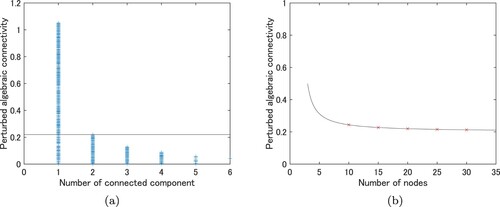
Here we demonstrate numerical examples of the condition Equation (11(11) ${\hat{\lambda }}^{\left(i\right)}>\frac{N}{5N-9},$(11) ). Figure 3(a) shows the perturbed algebraic connectivity ${\hat{\lambda }}^{\left(i\right)}$ of randomly generated graph with N = 20. The random graphs are generated by Erd$\stackrel{\mathrm{\prime }\mathrm{\prime }}{\mathrm{o}}$ s–Rényi model [11] with link probability 0.15, and link weights $a_{ij}$ are randomly chosen in the interval $(0,1)$. From Figure 3(a), we confirm that the computed perturbed algebraic connectivity ${\hat{\lambda }}^{\left(i\right)}$ (shown by the blue + marker) does not exceed $20/(5\times 20-9)\simeq 0.22$ (black line) if the node i is an articulation node. Additionally, we can see the inequality Equation (11(11) ${\hat{\lambda }}^{\left(i\right)}>\frac{N}{5N-9},$(11) ) is the sufficient condition, not a necessary condition for non-articulation nodes. Figure 3(b) shows numerical maximum of the perturbed algebraic connectivity ${\hat{\lambda }}^{\left(i\right)}$ when the node i is an articulation node. The red x markers indicate the numerical maximums and the black solid line shows the theoretical maximum $N/(5N-9)$. In each case, the theoretical maximum is approximately identical to the numerical maximum.

Figure 3. Numerical demonstration of sufficient condition Equation (11(11) ${\hat{\lambda }}^{\left(i\right)}>\frac{N}{5N-9},$(11) ). (a) ${\hat{\lambda }}^{\left(i\right)}$ v.s. # of connected component in ${\mathcal{G}}_{-i}$ and (b) Numerical maximum of ${\hat{\lambda }}^{\left(i\right)}$.

The control method we detail below switches two control modes: bi-connectivity preservation and bi-connectivity restoration. The preservation launches if all the perturbed algebraic connectivity ${\hat{\lambda }}^{\left(i\right)}$ satisfies the condition Equation (11(11) ${\hat{\lambda }}^{\left(i\right)}>\frac{N}{5N-9},$(11) ), and the restoration launches if one of the perturbed algebraic connectivity does not satisfy that condition. Note that the system does not detect whether a robot has failed but checks the perturbed algebraic connectivity of the non-failed robots. The bi-connectivity restoration could start even if the network is bi-connected since the inequality Equation (11(11) ${\hat{\lambda }}^{\left(i\right)}>\frac{N}{5N-9},$(11) ) is a sufficient condition. The restoration also could start if communication stops temporarily due to radio wave attenuation (e.g. fading). We can say that the system takes a safer policy.

3.2. Bi-connectivity preservation

Since the bi-connectedness is equivalent to the state that all the robot i are not articulation nodes, our control objective will be accomplished if we satisfy the condition Equation (11(11) ${\hat{\lambda }}^{\left(i\right)}>\frac{N}{5N-9},$(11) ) for all $i\in \mathcal{V}$. Here we propose two control methods: the robots preserve the condition Equation (11(11) ${\hat{\lambda }}^{\left(i\right)}>\frac{N}{5N-9},$(11) ) for all time if the condition is initially satisfied.

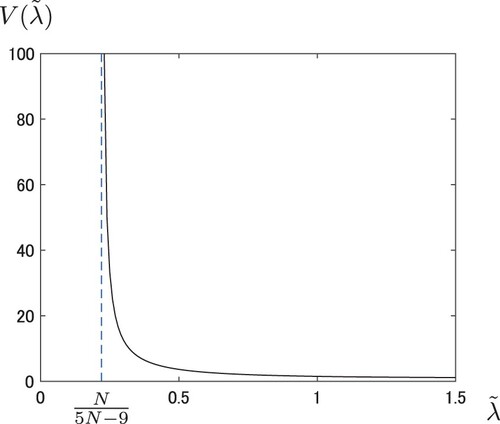
Inspired by a connectivity preserving control law proposed in the study [3], we define an artificial potential function $V\left({\tilde{\lambda }}^{\left(i\right)}\right)$ by (13) $V\left({\tilde{\lambda }}^{\left(i\right)}\right)=\mathrm{c}\mathrm{o}\mathrm{t}\mathrm{h}({\tilde{\lambda }}^{\left(i\right)}-N/(5N-9\left)\right),$(13) where $\mathrm{c}\mathrm{o}\mathrm{t}\mathrm{h}(\cdot )$ denotes the hyperbolic cotangent function (see Figure 4). Then we can ensure the condition Equation (11(11) ${\hat{\lambda }}^{\left(i\right)}>\frac{N}{5N-9},$(11) ) if the robots move in the gradient-decreasing direction.

Figure 4. Artificial potential function $V\left({\tilde{\lambda }}^{\left(i\right)}\right)$.

Theorem 3.2

Corollary of [3]

Assume the initial network $\mathcal{G}\left(0\right)$ consist of the initial robot positions $x_i\left(0\right)$ is bi-connected. If the bi-connectivity input $u_i^{\mathrm{b}\mathrm{c}}$ is given by (14) $u_i^{\mathrm{b}\mathrm{c}}=-\sum _{j\in \mathcal{V}}\frac{\mathrm{\partial }V\left({\tilde{\lambda }}^{\left(j\right)}\right)}{\mathrm{\partial }{x}_i},$(14) $k_i^{\mathrm{b}\mathrm{c}}>0$, $k_i^{\mathrm{t}\mathrm{a}\mathrm{s}\mathrm{k}}\ge 0$, and the task input is bounded $\Vert u_i^{\mathrm{t}\mathrm{a}\mathrm{s}\mathrm{k}}\Vert \le u_{max}$, then the network $\mathcal{G}\left(t\right)$ is bi-connected for all time t>0.

Proof.

This theorem is proved by showing the energy function $E\left(x\right)=\sum _{j}V\left({\tilde{\lambda }}^{\left(j\right)}\right(x\left)\right)$ is bounded for all time t, where x denotes the positions of all robots $x=[x_1^{\mathsf{T}},\dots ,x_N^{\mathsf{T}}{]}^{\mathsf{T}}$. First, the time derivative of the energy function E is given by (15) $\begin{array}{rl}\dot{E}& ={\left(\frac{\mathrm{\partial }E}{\mathrm{\partial }x}\right)}^{\mathsf{T}}\dot{x}={\left(\frac{\mathrm{\partial }E}{\mathrm{\partial }x}\right)}^{\mathsf{T}}(-\frac{\mathrm{\partial }E}{\mathrm{\partial }x}+k^{\mathrm{t}\mathrm{a}\mathrm{s}\mathrm{k}}{u}^{\mathrm{t}\mathrm{a}\mathrm{s}\mathrm{k}})\\ & \le -{\Vert \frac{\mathrm{\partial }E}{\mathrm{\partial }x}\Vert }^2+\Vert \frac{\mathrm{\partial }E}{\mathrm{\partial }x}\Vert u_{\mathrm{M}},\end{array}$(15) where $u^{\mathrm{t}\mathrm{a}\mathrm{s}\mathrm{k}}$ denotes the task input, $k^{\mathrm{t}\mathrm{a}\mathrm{s}\mathrm{k}}$ denotes the corresponding gain, and $u_M=max{k}^{\mathrm{t}\mathrm{a}\mathrm{s}\mathrm{k}}{u}^{\mathrm{t}\mathrm{a}\mathrm{s}\mathrm{k}}$. Then, the energy E may increase only when the inequality holds: (16) $\Vert \frac{\mathrm{\partial }E}{\mathrm{\partial }x}\Vert <u_{\mathrm{M}}.$(16) Here, the gradient $\mathrm{\partial }E/\mathrm{\partial }x=\left[\right(\mathrm{\partial }E/\mathrm{\partial }{x}_1{)}^{\mathsf{T}},\dots ,(\mathrm{\partial }E/\mathrm{\partial }{x}_N{)}^{\mathsf{T}}{]}^{\mathsf{T}}$ is given by (17) $\begin{array}{rl}\frac{\mathrm{\partial }E}{\mathrm{\partial }{x}_i}& =\sum _j\frac{\mathrm{\partial }V\left({\tilde{\lambda }}^{\left(j\right)}\right)}{\mathrm{\partial }{x}_i}=\sum _j\frac{\mathrm{\partial }V\left({\tilde{\lambda }}^{\left(j\right)}\right)}{\mathrm{\partial }{\tilde{\lambda }}^{\left(j\right)}}\frac{\mathrm{\partial }{\tilde{\lambda }}^{\left(j\right)}}{\mathrm{\partial }{x}_i}\\ & =-\sum _j{\mathrm{c}\mathrm{s}\mathrm{c}\mathrm{h}}^2({\tilde{\lambda }}^{\left(j\right)}-\overline{\lambda })\frac{\mathrm{\partial }{\tilde{\lambda }}^{\left(j\right)}}{\mathrm{\partial }{x}_i},\end{array}$(17) where $\mathrm{c}\mathrm{s}\mathrm{c}\mathrm{h}(\cdot )$ denotes the hyperbolic cosecant function, $\overline{\lambda }=N/(5N-9)$, and (18) $\begin{array}{rl}\frac{\mathrm{\partial }{\tilde{\lambda }}^{\left(j\right)}}{\mathrm{\partial }{x}_i}& =\frac{1}{ϵ}\frac{\mathrm{\partial }(v^{\left(j\right)}{)}^{\mathsf{T}}{L}^{\left(j\right)}{v}^{\left(j\right)}}{\mathrm{\partial }{x}_i}=\frac{1}{ϵ}(v^{\left(j\right)}{)}^{\mathsf{T}}\frac{\mathrm{\partial }{L}^{\left(j\right)}}{\mathrm{\partial }{x}_i}{v}^{\left(j\right)}\\ & =\frac{1}{ϵ}\sum _k(v_i^{\left(j\right)}-v_k^{\left(j\right)}{)}^2\frac{\mathrm{\partial }\left(a_{ik}^{\left(j\right)}/d_{jj}\right)}{\mathrm{\partial }{x}_i},\end{array}$(18) from ${\tilde{\lambda }}^{\left(j\right)}={\lambda }_2^{\left(j\right)}/ϵ$. Note that $\mathrm{\partial }{\tilde{\lambda }}^{\left(j\right)}/\mathrm{\partial }{x}_j\ne 0$. From above, there exists a positive value c such that (19) ${\mathrm{c}\mathrm{s}\mathrm{c}\mathrm{h}}^2({\tilde{\lambda }}^{\left(j\right)}-\overline{\lambda })<c,\mathrm{\forall }j\in \mathcal{V},$(19) when $\dot{E}>0$, and clearly this is also hold when $\dot{E}\le 0$. Thus ${\tilde{\lambda }}^{\left(j\right)}>\overline{\lambda }$ for all node j and for all time t.

Using the expression Equation (18(18) $\begin{array}{rl}\frac{\mathrm{\partial }{\tilde{\lambda }}^{\left(j\right)}}{\mathrm{\partial }{x}_i}& =\frac{1}{ϵ}\frac{\mathrm{\partial }(v^{\left(j\right)}{)}^{\mathsf{T}}{L}^{\left(j\right)}{v}^{\left(j\right)}}{\mathrm{\partial }{x}_i}=\frac{1}{ϵ}(v^{\left(j\right)}{)}^{\mathsf{T}}\frac{\mathrm{\partial }{L}^{\left(j\right)}}{\mathrm{\partial }{x}_i}{v}^{\left(j\right)}\\ & =\frac{1}{ϵ}\sum _k(v_i^{\left(j\right)}-v_k^{\left(j\right)}{)}^2\frac{\mathrm{\partial }\left(a_{ik}^{\left(j\right)}/d_{jj}\right)}{\mathrm{\partial }{x}_i},\end{array}$(18) ), the control input Equation (14(14) $u_i^{\mathrm{b}\mathrm{c}}=-\sum _{j\in \mathcal{V}}\frac{\mathrm{\partial }V\left({\tilde{\lambda }}^{\left(j\right)}\right)}{\mathrm{\partial }{x}_i},$(14) ) is rewritten by (20) $\begin{array}{rl}{u}_i^{\mathrm{b}\mathrm{c}}& =\sum _{j\in \mathcal{V}}{\mathrm{c}\mathrm{s}\mathrm{c}\mathrm{h}}^2({\tilde{\lambda }}^{\left(j\right)}-N/(5N-9\left)\right)\\ & \times \sum _{k\in {\mathcal{N}}_i}\frac{{(v_i^{\left(j\right)}-v_k^{\left(j\right)})}^2}{ϵ}\frac{\mathrm{\partial }\left(a_{ik}^{\left(j\right)}/d_{jj}\right)}{\mathrm{\partial }{x}_i},\end{array}$(20) where (21) $\frac{\mathrm{\partial }\left(a_{ik}^{\left(j\right)}/d_{jj}\right)}{\mathrm{\partial }{x}_i}=\{\begin{array}{ll}{\displaystyle ϵ\frac{d_{jj}-a_{ik}}{d_{jj}^2}\frac{\mathrm{\partial }{a}_{ik}}{\mathrm{\partial }{x}_i},}& \mathrm{i}\mathrm{f}i=j\mathrm{o}\mathrm{r}k=j,\\ {\displaystyle \frac{1}{d_{jj}}\frac{\mathrm{\partial }{a}_{ik}}{\mathrm{\partial }{x}_i},}& \mathrm{o}\mathrm{t}\mathrm{h}\mathrm{e}\mathrm{r}\mathrm{w}\mathrm{i}\mathrm{s}\mathrm{e}.\end{array}$(21) The control input Equation (20(20) $\begin{array}{rl}{u}_i^{\mathrm{b}\mathrm{c}}& =\sum _{j\in \mathcal{V}}{\mathrm{c}\mathrm{s}\mathrm{c}\mathrm{h}}^2({\tilde{\lambda }}^{\left(j\right)}-N/(5N-9\left)\right)\\ & \times \sum _{k\in {\mathcal{N}}_i}\frac{{(v_i^{\left(j\right)}-v_k^{\left(j\right)})}^2}{ϵ}\frac{\mathrm{\partial }\left(a_{ik}^{\left(j\right)}/d_{jj}\right)}{\mathrm{\partial }{x}_i},\end{array}$(20) ) requires the local information $a_{ik}$ and $\mathrm{\partial }{a}_{ik}/\mathrm{\partial }{x}_i$, the perturbed eigenpair ${\tilde{\lambda }}^{\left(j\right)}$ and $v^{\left(j\right)}$ which is estimated by the distributed algorithm [7], and the degree $d_{jj}$ for the normalization. Although the degree $d_{jj}$ is not the local information, all the robots j can modify the elements of the perturbed Laplacian matrix $L^{\left(j\right)}$ to be $d_{jj}=1$ in a distributed manner.

3.3. Bi-connectivity restoration

Similarly, the robots will resume the condition Equation (11(11) ${\hat{\lambda }}^{\left(i\right)}>\frac{N}{5N-9},$(11) ) by moving in the gradient increasing direction if the condition is not satisfied initially. We analysed a condition to resume the network bi-connected.

Theorem 3.3

Assume the initial network $\mathcal{G}\left(0\right)$ consist of the initial robot positions $x_i\left(0\right)$ is uni-connected, all distances ${\mathrm{d}\mathrm{i}\mathrm{s}\mathrm{t}}_{ijk}$ from obstacles $k\in \mathcal{O}$ to segments $\mathrm{s}\mathrm{e}\mathrm{g}(x_i,x_j)$ are greater than $d_{max}$, and the convex hull $\mathcal{C}$ consist of the initial robot positions $x_i\left(0\right)$ does not contain any obstacles $k\in \mathcal{O}$. If the bi-connectivity input $u_i^{\mathrm{b}\mathrm{c}}$ is given by (22) $u_i^{\mathrm{b}\mathrm{c}}=k^{\mathrm{r}\mathrm{e}\mathrm{s}\mathrm{t}\mathrm{o}\mathrm{r}\mathrm{e}}\sum _{j\in {\mathcal{V}}_a}\frac{\mathrm{\partial }{\tilde{\lambda }}^{\left(j\right)}}{\mathrm{\partial }{x}_i}-\sum _{j\in \mathcal{V}\setminus {\mathcal{V}}_a}\frac{\mathrm{\partial }V\left({\tilde{\lambda }}^{\left(j\right)}\right)}{\mathrm{\partial }{x}_i},$(22) where ${\mathcal{V}}_a=\{j\in \mathcal{V}|{\tilde{\lambda }}^{\left(j\right)}<N/(5N-9)\wedge j\mathrm{h}\mathrm{a}\mathrm{s}\ge 2\mathrm{l}\mathrm{i}\mathrm{n}\mathrm{k}\mathrm{s}\}$, and gains are $k^{\mathrm{r}\mathrm{e}\mathrm{s}\mathrm{t}\mathrm{o}\mathrm{r}\mathrm{e}}>0$, $k_i^{\mathrm{b}\mathrm{c}}>0$, $k_i^{\mathrm{t}\mathrm{a}\mathrm{s}\mathrm{k}}=0$, then the network $\mathcal{G}\left(t\right)$ becomes bi-connected in finite time $t^{\prime }>0$.

Proof.

Under the assumption, the robotic system Equation (1(1) ${\dot{x}}_i\left(t\right)=k_i^{\mathrm{b}\mathrm{c}}{u}_i^{\mathrm{b}\mathrm{c}}\left(t\right)+k_i^{\mathrm{t}\mathrm{a}\mathrm{s}\mathrm{k}}{u}_i^{\mathrm{t}\mathrm{a}\mathrm{s}\mathrm{k}}\left(t\right),$(1) ) can be rewritten as (23) $\begin{array}{rl}{\dot{x}}_i& =\sum _{j\in \mathcal{V}}{g}_j\sum _{k\in {\mathcal{N}}_i}\frac{(v_i^{\left(j\right)}-v_k^{\left(j\right)}{)}^2}{ϵ}\frac{\mathrm{\partial }{a}_{ik}^{\left(j\right)}}{\mathrm{\partial }{x}_i}\\ & =\sum _{k\in {\mathcal{N}}_i}\left(\sum _{j\in \mathcal{V}}{g}_j\frac{(v_i^{\left(j\right)}-v_k^{\left(j\right)}{)}^2}{ϵ}{d}_{ik}^{\left(j\right)}\right)\frac{\mathrm{\partial }{a}_{ik}}{\mathrm{\partial }{x}_i},\end{array}$(23) where $v_i^{\left(j\right)}$ denotes the ith element of the eigenvector $v^{\left(j\right)}$ w.r.t. the eigenvalue ${\lambda }_2^{\left(j\right)}\left(ϵ\right)$, and (24) $\begin{array}{rl}{g}_j& =\{\begin{array}{ll}{k}^{\mathrm{r}\mathrm{e}\mathrm{s}\mathrm{t}\mathrm{o}\mathrm{r}\mathrm{e}},& \mathrm{i}\mathrm{f}j\in {\mathcal{V}}_a,\\ {\mathrm{c}\mathrm{s}\mathrm{c}\mathrm{h}}^2({\tilde{\lambda }}^{\left(j\right)}-N/(5N-9\left)\right),& \mathrm{o}\mathrm{t}\mathrm{h}\mathrm{e}\mathrm{r}\mathrm{w}\mathrm{i}\mathrm{s}\mathrm{e},\end{array}\end{array}$(24) (25) $\begin{array}{rl}{d}_{ik}^{\left(j\right)}& =\{\begin{array}{ll}{\displaystyle ϵ\frac{d_{jj}-a_{ik}}{d_{jj}^2},}& \mathrm{i}\mathrm{f}i=j\mathrm{o}\mathrm{r}k=j,\\ {\displaystyle \frac{1}{d_{jj}},}& \mathrm{o}\mathrm{t}\mathrm{h}\mathrm{e}\mathrm{r}\mathrm{w}\mathrm{i}\mathrm{s}\mathrm{e}.\end{array}\end{array}$(25) Here we can see (26) $\begin{array}{rl}& \sum _{j\in \mathcal{V}}{g}_j\frac{(v_i^{\left(j\right)}-v_k^{\left(j\right)}{)}^2}{ϵ}{d}_{ik}^{\left(j\right)}\ge g_i\frac{d_{ii}-a_{ik}}{d_{ii}}(v_i^{\left(i\right)}-v_k^{\left(i\right)}{)}^2\\ & +g_k\frac{d_{kk}-a_{ik}}{d_{kk}}(v_i^{\left(k\right)}-v_k^{\left(k\right)}{)}^2>0.\end{array}$(26) Next, the gradient $\mathrm{\partial }{a}_{ik}/\mathrm{\partial }{x}_i$ is expressed by (27) $\frac{\mathrm{\partial }{a}_{ik}}{\mathrm{\partial }{x}_i}=\frac{\alpha \exp (-\alpha ({\mathrm{d}\mathrm{i}\mathrm{s}\mathrm{t}}_{ik}/R-\text{β}\left)\right)}{R(1+\exp (-\alpha ({\mathrm{d}\mathrm{i}\mathrm{s}\mathrm{t}}_{ik}/R-\text{β})\left)\right)}\frac{x_k-x_i}{{\mathrm{d}\mathrm{i}\mathrm{s}\mathrm{t}}_{ik}},$(27) from the definition Equation (3(3) ${\gamma }^a\left({\mathrm{d}\mathrm{i}\mathrm{s}\mathrm{t}}_{ij}\right)=1-{(1+\exp (-{\alpha }_a(\frac{{\mathrm{d}\mathrm{i}\mathrm{s}\mathrm{t}}_{ij}}{R}-{\text{β}}_a)))}^{-1},$(3) ). Thus we can rewrite Equation (23(23) $\begin{array}{rl}{\dot{x}}_i& =\sum _{j\in \mathcal{V}}{g}_j\sum _{k\in {\mathcal{N}}_i}\frac{(v_i^{\left(j\right)}-v_k^{\left(j\right)}{)}^2}{ϵ}\frac{\mathrm{\partial }{a}_{ik}^{\left(j\right)}}{\mathrm{\partial }{x}_i}\\ & =\sum _{k\in {\mathcal{N}}_i}\left(\sum _{j\in \mathcal{V}}{g}_j\frac{(v_i^{\left(j\right)}-v_k^{\left(j\right)}{)}^2}{ϵ}{d}_{ik}^{\left(j\right)}\right)\frac{\mathrm{\partial }{a}_{ik}}{\mathrm{\partial }{x}_i},\end{array}$(23) ) as (28) ${\dot{x}}_i=\sum _{k\in {\mathcal{N}}_i}{b}_{ik}(x_k-x_i),$(28) by defining an appropriate strictly positive variable $b_{ik}>0$. Note this dynamics is a consensus algorithm [12]. Therefore, we can see all the points $x_i$ are in the convex hull $\mathcal{C}$ and move towards the consensus set $\mathcal{X}=\{x\in {\mathbf{R}}^{dN}|x_i=x_j,\mathrm{\forall }i,j\}$. Figure 5 illustrates this behaviour. The system state $x\left(t\right)$ approaches to the consensus set $\mathcal{X}$ and the bi-connectedness is resumed at finite time $t^{\prime }$.

Figure 5. Robots on boundary of convex hull $\mathcal{C}$ move into $\mathcal{C}$.

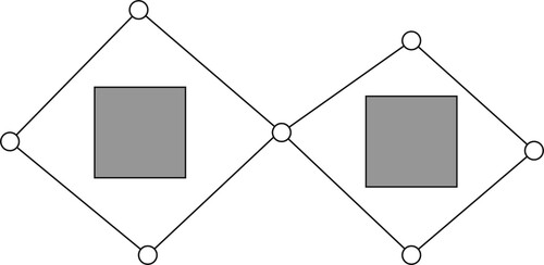
The above theorem ensures the achievement of the bi-connectivity restoration only under some initial configurations of the robots. Unfortunately in cases that the convex hull $\mathcal{C}$ contains some obstacles, the multi-robot system falls into a local optimum and the bi-connectedness may not be restored. For instance, the robots which move from the initial positions described in Figure 6 cannot resume the bi-conectedness of the network while preserving all other non-articulation nodes. The local optimum set to be avoided for the bi-connectivity restoration is expressed by (29) $\begin{array}{rl}\mathcal{L}& =\{x\in {\mathbf{R}}^{dN}|\mathrm{r}\mathrm{i}\mathrm{g}\mathrm{h}\mathrm{t}\mathrm{h}\mathrm{a}\mathrm{n}\mathrm{d}\mathrm{o}\mathrm{f}\mathrm{E}\mathrm{q}\mathrm{u}\mathrm{a}\mathrm{t}\mathrm{i}\mathrm{o}\mathrm{n}(22)=0,\mathrm{\forall }i,\\ & \mathrm{a}\mathrm{n}\mathrm{d}\mathrm{\exists }j\mathrm{s}.\mathrm{t}.{\tilde{\lambda }}^{\left(j\right)}\le N/(5N-9)\}.\end{array}$(29) In other words, the restoration control Equation (22(22) $u_i^{\mathrm{b}\mathrm{c}}=k^{\mathrm{r}\mathrm{e}\mathrm{s}\mathrm{t}\mathrm{o}\mathrm{r}\mathrm{e}}\sum _{j\in {\mathcal{V}}_a}\frac{\mathrm{\partial }{\tilde{\lambda }}^{\left(j\right)}}{\mathrm{\partial }{x}_i}-\sum _{j\in \mathcal{V}\setminus {\mathcal{V}}_a}\frac{\mathrm{\partial }V\left({\tilde{\lambda }}^{\left(j\right)}\right)}{\mathrm{\partial }{x}_i},$(22) ) will make the network bi-connected if the system state $x\left(t\right)$ is not in the local optimum set $\mathcal{L}$ for all time t.

Figure 6. Difficult situation to resume bi-connectivity while keeping other non-articulation nodes.

3.3.1. Avoiding local optimum

To avoid such local minima and to encourage resuming the bi-connectivity, we propose a heuristic technique that temporally stops the preserving control (second term of Equation (22(22) $u_i^{\mathrm{b}\mathrm{c}}=k^{\mathrm{r}\mathrm{e}\mathrm{s}\mathrm{t}\mathrm{o}\mathrm{r}\mathrm{e}}\sum _{j\in {\mathcal{V}}_a}\frac{\mathrm{\partial }{\tilde{\lambda }}^{\left(j\right)}}{\mathrm{\partial }{x}_i}-\sum _{j\in \mathcal{V}\setminus {\mathcal{V}}_a}\frac{\mathrm{\partial }V\left({\tilde{\lambda }}^{\left(j\right)}\right)}{\mathrm{\partial }{x}_i},$(22) )) considering that the preservation term disturbs the bi-connectivity restoration. The restoration control input Equation (22(22) $u_i^{\mathrm{b}\mathrm{c}}=k^{\mathrm{r}\mathrm{e}\mathrm{s}\mathrm{t}\mathrm{o}\mathrm{r}\mathrm{e}}\sum _{j\in {\mathcal{V}}_a}\frac{\mathrm{\partial }{\tilde{\lambda }}^{\left(j\right)}}{\mathrm{\partial }{x}_i}-\sum _{j\in \mathcal{V}\setminus {\mathcal{V}}_a}\frac{\mathrm{\partial }V\left({\tilde{\lambda }}^{\left(j\right)}\right)}{\mathrm{\partial }{x}_i},$(22) ) is modified as (30) $u_i^{\mathrm{b}\mathrm{c}}=\{\begin{array}{ll}\begin{array}{l}{\displaystyle k^{\mathrm{r}\mathrm{e}\mathrm{s}\mathrm{t}\mathrm{o}\mathrm{r}\mathrm{e}}\sum _{j\in {\mathcal{V}}_a}\frac{\mathrm{\partial }{\tilde{\lambda }}^{\left(j\right)}}{\mathrm{\partial }{x}_i}}\\ -\sum _{j\in \mathcal{V}\setminus {\mathcal{V}}_a}\frac{\mathrm{\partial }V\left({\tilde{\lambda }}^{\left(j\right)}\right)}{\mathrm{\partial }{x}_i},\end{array}& \mathrm{i}\mathrm{f}{\displaystyle \underset{j}{max}{t}_j<\overline{t},}\\ {\displaystyle k^{\mathrm{r}\mathrm{e}\mathrm{s}\mathrm{t}\mathrm{o}\mathrm{r}\mathrm{e}}\sum _{j\in \mathcal{V}}\frac{\mathrm{\partial }{\tilde{\lambda }}^{\left(j\right)}}{\mathrm{\partial }{x}_i},}& \mathrm{o}\mathrm{t}\mathrm{h}\mathrm{e}\mathrm{r}\mathrm{w}\mathrm{i}\mathrm{s}\mathrm{e},\end{array}$(30) where $\overline{t}$ denotes the time threshold to preserve non-articulation nodes and $t_i$ denotes the preserving time count. The parameter $t_i$ changes as below: (31) $\{\begin{array}{ll}{\dot{t}}_i=1,& \mathrm{i}\mathrm{f}{\tilde{\lambda }}^{\left(i\right)}\le N/(5N-9)+\delta ,\\ t_i=0,& \mathrm{o}\mathrm{t}\mathrm{h}\mathrm{e}\mathrm{r}\mathrm{w}\mathrm{i}\mathrm{s}\mathrm{e},\end{array}$(31) where $\delta >0$ denotes a small margin not to let ${\tilde{\lambda }}^{\left(i\right)}$ be too large. The time threshold $\overline{t}$ is set to be sufficiently large so that $\underset{j}{max}{t}_j$ becomes larger than $\overline{t}$ only when the system state x is close to the local optimum set $\mathcal{L}$.

A rough outline of this control law Equation (30(30) $u_i^{\mathrm{b}\mathrm{c}}=\{\begin{array}{ll}\begin{array}{l}{\displaystyle k^{\mathrm{r}\mathrm{e}\mathrm{s}\mathrm{t}\mathrm{o}\mathrm{r}\mathrm{e}}\sum _{j\in {\mathcal{V}}_a}\frac{\mathrm{\partial }{\tilde{\lambda }}^{\left(j\right)}}{\mathrm{\partial }{x}_i}}\\ -\sum _{j\in \mathcal{V}\setminus {\mathcal{V}}_a}\frac{\mathrm{\partial }V\left({\tilde{\lambda }}^{\left(j\right)}\right)}{\mathrm{\partial }{x}_i},\end{array}& \mathrm{i}\mathrm{f}{\displaystyle \underset{j}{max}{t}_j<\overline{t},}\\ {\displaystyle k^{\mathrm{r}\mathrm{e}\mathrm{s}\mathrm{t}\mathrm{o}\mathrm{r}\mathrm{e}}\sum _{j\in \mathcal{V}}\frac{\mathrm{\partial }{\tilde{\lambda }}^{\left(j\right)}}{\mathrm{\partial }{x}_i},}& \mathrm{o}\mathrm{t}\mathrm{h}\mathrm{e}\mathrm{r}\mathrm{w}\mathrm{i}\mathrm{s}\mathrm{e},\end{array}$(30) ) is given as below. The non-articulation preserving mode (the first line of Equation (30(30) $u_i^{\mathrm{b}\mathrm{c}}=\{\begin{array}{ll}\begin{array}{l}{\displaystyle k^{\mathrm{r}\mathrm{e}\mathrm{s}\mathrm{t}\mathrm{o}\mathrm{r}\mathrm{e}}\sum _{j\in {\mathcal{V}}_a}\frac{\mathrm{\partial }{\tilde{\lambda }}^{\left(j\right)}}{\mathrm{\partial }{x}_i}}\\ -\sum _{j\in \mathcal{V}\setminus {\mathcal{V}}_a}\frac{\mathrm{\partial }V\left({\tilde{\lambda }}^{\left(j\right)}\right)}{\mathrm{\partial }{x}_i},\end{array}& \mathrm{i}\mathrm{f}{\displaystyle \underset{j}{max}{t}_j<\overline{t},}\\ {\displaystyle k^{\mathrm{r}\mathrm{e}\mathrm{s}\mathrm{t}\mathrm{o}\mathrm{r}\mathrm{e}}\sum _{j\in \mathcal{V}}\frac{\mathrm{\partial }{\tilde{\lambda }}^{\left(j\right)}}{\mathrm{\partial }{x}_i},}& \mathrm{o}\mathrm{t}\mathrm{h}\mathrm{e}\mathrm{r}\mathrm{w}\mathrm{i}\mathrm{s}\mathrm{e},\end{array}$(30) )) is stopped when the state x is trapped by the local optima $\mathcal{L}$, and the local optima avoiding mode (the second line of Equation (30(30) $u_i^{\mathrm{b}\mathrm{c}}=\{\begin{array}{ll}\begin{array}{l}{\displaystyle k^{\mathrm{r}\mathrm{e}\mathrm{s}\mathrm{t}\mathrm{o}\mathrm{r}\mathrm{e}}\sum _{j\in {\mathcal{V}}_a}\frac{\mathrm{\partial }{\tilde{\lambda }}^{\left(j\right)}}{\mathrm{\partial }{x}_i}}\\ -\sum _{j\in \mathcal{V}\setminus {\mathcal{V}}_a}\frac{\mathrm{\partial }V\left({\tilde{\lambda }}^{\left(j\right)}\right)}{\mathrm{\partial }{x}_i},\end{array}& \mathrm{i}\mathrm{f}{\displaystyle \underset{j}{max}{t}_j<\overline{t},}\\ {\displaystyle k^{\mathrm{r}\mathrm{e}\mathrm{s}\mathrm{t}\mathrm{o}\mathrm{r}\mathrm{e}}\sum _{j\in \mathcal{V}}\frac{\mathrm{\partial }{\tilde{\lambda }}^{\left(j\right)}}{\mathrm{\partial }{x}_i},}& \mathrm{o}\mathrm{t}\mathrm{h}\mathrm{e}\mathrm{r}\mathrm{w}\mathrm{i}\mathrm{s}\mathrm{e},\end{array}$(30) )) will be executed until the node becomes non-articulation. Since it is difficult to observe that the state x is close to the local optimal set $\mathcal{L}$ in a distributed fashion, instead we employ the length of time the bi-connectivity has not been restored. By stopping the non-articulation node preservation condition (11(11) ${\hat{\lambda }}^{\left(i\right)}>\frac{N}{5N-9},$(11) ), we try to force the state x to escape from the set $\mathcal{L}$.

The state trajectory $x\left(t\right)$ of the system Equation (1(1) ${\dot{x}}_i\left(t\right)=k_i^{\mathrm{b}\mathrm{c}}{u}_i^{\mathrm{b}\mathrm{c}}\left(t\right)+k_i^{\mathrm{t}\mathrm{a}\mathrm{s}\mathrm{k}}{u}_i^{\mathrm{t}\mathrm{a}\mathrm{s}\mathrm{k}}\left(t\right),$(1) ) with the control law Equation (30(30) $u_i^{\mathrm{b}\mathrm{c}}=\{\begin{array}{ll}\begin{array}{l}{\displaystyle k^{\mathrm{r}\mathrm{e}\mathrm{s}\mathrm{t}\mathrm{o}\mathrm{r}\mathrm{e}}\sum _{j\in {\mathcal{V}}_a}\frac{\mathrm{\partial }{\tilde{\lambda }}^{\left(j\right)}}{\mathrm{\partial }{x}_i}}\\ -\sum _{j\in \mathcal{V}\setminus {\mathcal{V}}_a}\frac{\mathrm{\partial }V\left({\tilde{\lambda }}^{\left(j\right)}\right)}{\mathrm{\partial }{x}_i},\end{array}& \mathrm{i}\mathrm{f}{\displaystyle \underset{j}{max}{t}_j<\overline{t},}\\ {\displaystyle k^{\mathrm{r}\mathrm{e}\mathrm{s}\mathrm{t}\mathrm{o}\mathrm{r}\mathrm{e}}\sum _{j\in \mathcal{V}}\frac{\mathrm{\partial }{\tilde{\lambda }}^{\left(j\right)}}{\mathrm{\partial }{x}_i},}& \mathrm{o}\mathrm{t}\mathrm{h}\mathrm{e}\mathrm{r}\mathrm{w}\mathrm{i}\mathrm{s}\mathrm{e},\end{array}$(30) ) and $u_i^{\mathrm{t}\mathrm{a}\mathrm{s}\mathrm{k}}=0$ does not converge any closed cycles, under the assumption: (32) $\begin{array}{rl}& k^{\mathrm{r}\mathrm{e}\mathrm{s}\mathrm{t}\mathrm{o}\mathrm{r}\mathrm{e}}(\mu -\nu )\ge -\left(V\right(\mu )-V(\nu \left)\right),\\ & \mathrm{\forall }\mu ,\nu \ge N/(5N-9)+\delta .\end{array}$(32) This fact is confirmed by showing that the summation of the perturbed algebraic connectivity $\mathrm{\Lambda }=\sum _i{\tilde{\lambda }}^{\left(i\right)}$ does not decrease over time t. Defining the energy function $E\left(t\right)=k^{\mathrm{r}\mathrm{e}\mathrm{s}\mathrm{t}\mathrm{o}\mathrm{r}\mathrm{e}}\sum _{j\in {\mathcal{V}}_a}{\tilde{\lambda }}^{\left(j\right)}\left(t\right)-\sum _{j\in \mathcal{V}\setminus {\mathcal{V}}_a}V\left({\tilde{\lambda }}^{\left(j\right)}\right(t\left)\right)$, the non-articulation preservation mode does not reduce the energy $E\left(t\right)$, that is, $E\left(t\right)-E\left(0\right)\ge 0$ for all t>0. From a simple deformation: (33) $\begin{array}{rl}E\left(t\right)-E\left(0\right)& =k^{\mathrm{r}\mathrm{e}\mathrm{s}\mathrm{t}\mathrm{o}\mathrm{r}\mathrm{e}}\sum _{j\in {\mathcal{V}}_a}\left({\tilde{\lambda }}^{\left(j\right)}\right(t)-{\tilde{\lambda }}^{\left(j\right)}(0\left)\right)\\ & -\sum _{j\in \mathcal{V}\setminus {\mathcal{V}}_a}\left(V\right({\tilde{\lambda }}^{\left(j\right)}\left(t\right))-V({\tilde{\lambda }}^{\left(j\right)}\left(0\right)\left)\right),\end{array}$(33) we get $\mathrm{\Lambda }\left(t\right)-\mathrm{\Lambda }\left(0\right)\ge 0$ for all t>0. Thus, the system trajectory $x\left(t\right)$ results in either achievement of the bi-connectivity restoration or convergence towards the alternative local optimum set (34) $\begin{array}{rl}{\mathcal{L}}^{\prime }& =\{x\in {\mathbf{R}}^{dN}|\mathrm{\partial }\mathrm{\Lambda }/\mathrm{\partial }{x}_i=0,\mathrm{\forall }i,\\ & \mathrm{a}\mathrm{n}\mathrm{d}\mathrm{\exists }j\mathrm{s}.\mathrm{t}.{\tilde{\lambda }}^{\left(j\right)}\le N/(5N-9)\},\end{array}$(34) to be avoided. We may be able to avoid this local optimal set ${\mathcal{L}}^{\prime }$ by switching the control mode if $\mathcal{L}\cap {\mathcal{L}}^{\prime }=\mathrm{\varnothing }$. Further analysis and improving the control law remain future works.

4. Numerical simulations

In this section, numerical simulations are demonstrated to describe the usefulness of the proposed method. The task control input $u_i^{\mathrm{t}\mathrm{a}\mathrm{s}\mathrm{k}}$ is given by (35) $u_i^{\mathrm{t}\mathrm{a}\mathrm{s}\mathrm{k}}=\sum _{j\in {\mathcal{N}}_i}\frac{x_i-x_j}{\Vert x_i-x_j\Vert },$(35) considering a coverage control. The perturbation parameter ε is $ϵ=0.01$, and the control gains are $k_i^{\mathrm{b}\mathrm{c}}=1,k_i^{\mathrm{t}\mathrm{a}\mathrm{s}\mathrm{k}}=1,$ and $k^{\mathrm{r}\mathrm{e}\mathrm{s}\mathrm{t}\mathrm{o}\mathrm{r}\mathrm{e}}={10}^5$. The control input $u_i$ is saturated as $0.2u_i/\Vert u_i\Vert$ if $\Vert u_i\Vert >0.2$. The number of robotic-nodes is N = 20. The parameters of the link weight $a_{ij}$ are defined in Equations (3(3) ${\gamma }^a\left({\mathrm{d}\mathrm{i}\mathrm{s}\mathrm{t}}_{ij}\right)=1-{(1+\exp (-{\alpha }_a(\frac{{\mathrm{d}\mathrm{i}\mathrm{s}\mathrm{t}}_{ij}}{R}-{\text{β}}_a)))}^{-1},$(3) ) and (4(4) ${\gamma }^b\left({\mathrm{d}\mathrm{i}\mathrm{s}\mathrm{t}}_{ijk}\right)={(1+\exp (-{\alpha }_b(\frac{{\mathrm{d}\mathrm{i}\mathrm{s}\mathrm{t}}_{ijk}}{d_{max}}-{\text{β}}_b)))}^{-1},$(4) ) are set by $\alpha =40$ and $\text{β}=0.75$.

We show a simulation result of the restoration control Equation (22(22) $u_i^{\mathrm{b}\mathrm{c}}=k^{\mathrm{r}\mathrm{e}\mathrm{s}\mathrm{t}\mathrm{o}\mathrm{r}\mathrm{e}}\sum _{j\in {\mathcal{V}}_a}\frac{\mathrm{\partial }{\tilde{\lambda }}^{\left(j\right)}}{\mathrm{\partial }{x}_i}-\sum _{j\in \mathcal{V}\setminus {\mathcal{V}}_a}\frac{\mathrm{\partial }V\left({\tilde{\lambda }}^{\left(j\right)}\right)}{\mathrm{\partial }{x}_i},$(2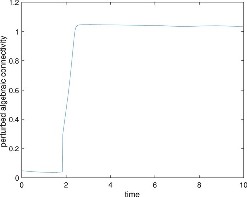2) ). Figure 7 represents snapshots of the initial configuration t = 0 (Figure 7(a)), at time t = 1.9 when the bi-connectivity is restored (Figure 7(b)), and at time t = 10 when the multi-robot system converges a stable state (Figure 7(c)). Figure 8 represents the approximated perturbed algebraic connectivity ${\tilde{\lambda }}^{\left(20\right)}$ where the node 20 is initially an articulation one ($x_{20}\left(0\right)=(0,0{)}^{\mathrm{\top }}$on Figure 7(a)). We can confirm that the algebraic connectivity ${\tilde{\lambda }}^{\left(20\right)}$ increases and is greater than $N/(5N-9)\simeq 0.22$ after t = 1.9. This indicates the proposed control law Equation (22(22) $u_i^{\mathrm{b}\mathrm{c}}=k^{\mathrm{r}\mathrm{e}\mathrm{s}\mathrm{t}\mathrm{o}\mathrm{r}\mathrm{e}}\sum _{j\in {\mathcal{V}}_a}\frac{\mathrm{\partial }{\tilde{\lambda }}^{\left(j\right)}}{\mathrm{\partial }{x}_i}-\sum _{j\in \mathcal{V}\setminus {\mathcal{V}}_a}\frac{\mathrm{\partial }V\left({\tilde{\lambda }}^{\left(j\right)}\right)}{\mathrm{\partial }{x}_i},$(22) ) restores the bi-connectivity of the network and Equation (14(14) $u_i^{\mathrm{b}\mathrm{c}}=-\sum _{j\in \mathcal{V}}\frac{\mathrm{\partial }V\left({\tilde{\lambda }}^{\left(j\right)}\right)}{\mathrm{\partial }{x}_i},$(14) ) preserves it.

Figure 7. Snapshots of simulation 1. (a) Initial configuration (t = 0). (b) Node 20 is restored at t = 1.9 and (c) Final configuration at t = 10.

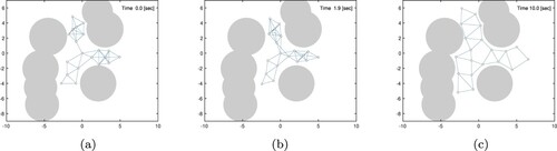
Figure 8. Perturbed algebraic connectivity ${\tilde{\lambda }}^{\left(20\right)}$ versus time t.

Next, we examine the effects of the modified restoration algorithm Equation (30(30) $u_i^{\mathrm{b}\mathrm{c}}=\{\begin{array}{ll}\begin{array}{l}{\displaystyle k^{\mathrm{r}\mathrm{e}\mathrm{s}\mathrm{t}\mathrm{o}\mathrm{r}\mathrm{e}}\sum _{j\in {\mathcal{V}}_a}\frac{\mathrm{\partial }{\tilde{\lambda }}^{\left(j\right)}}{\mathrm{\partial }{x}_i}}\\ -\sum _{j\in \mathcal{V}\setminus {\mathcal{V}}_a}\frac{\mathrm{\partial }V\left({\tilde{\lambda }}^{\left(j\right)}\right)}{\mathrm{\partial }{x}_i},\end{array}& \mathrm{i}\mathrm{f}{\displaystyle \underset{j}{max}{t}_j<\overline{t},}\\ {\displaystyle k^{\mathrm{r}\mathrm{e}\mathrm{s}\mathrm{t}\mathrm{o}\mathrm{r}\mathrm{e}}\sum _{j\in \mathcal{V}}\frac{\mathrm{\partial }{\tilde{\lambda }}^{\left(j\right)}}{\mathrm{\partial }{x}_i},}& \mathrm{o}\mathrm{t}\mathrm{h}\mathrm{e}\mathrm{r}\mathrm{w}\mathrm{i}\mathrm{s}\mathrm{e},\end{array}$(30) ). The time threshold $\overline{t}$ is set as $\overline{t}=10$. 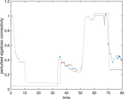Figure 9 represents snapshots of the initial configuration t = 0 (Figure 9(a)), at time t = 20 when the robots move to restore the bi-connectivity (Figure 9(b)), and at time t = 80 when the bi-connectivity is restored (Figure 9(c)). Figure 10 represents the approximated perturbed algebraic connectivity ${\tilde{\lambda }}^{\left(20\right)}$ and ${\tilde{\lambda }}^{\left(1\right)}$, where node 20 is an articulation and node 1 is not an articulation initially. We can confirm that the algebraic connectivity ${\tilde{\lambda }}^{\left(20\right)}$ increases and greater than $N/(5N-9)\simeq 0.22$ after t = 30. The algebraic connectivity ${\tilde{\lambda }}^{\left(1\right)}$ once becomes less than $N/(5N-9)\simeq 0.22$ at t = 10 and becomes greater than $N/(5N-9)\simeq 0.22$ after t = 30. It indicates that node 1 becomes an articulation node once to robustify the network structure around node 20, and it resumes itself after node 20 becomes a non-articulation one.

Figure 9. Snapshots of simulation 2. (a) Initial configuration (t = 0). (b) t = 20 and (c) t = 80.

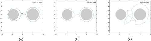
Figure 10. Perturbed algebraic connectivities ${\tilde{\lambda }}^{\left(20\right)}$ (blue line) and ${\tilde{\lambda }}^{\left(1\right)}$ (red line) versus time t. Node 1 is initially non-articulation but becomes an articulation node to restore the bi-connectivity of the entire network.

5. Conclusion

In this paper, we proposed control methods to preserve and restore the bi-connectivity of the multi-robot network, in preparation for a failure of the robot. We introduced the concept of perturbed algebraic connectivity which reflects the connectivity of the graph after a node is removed, and we considered an artificial potential control to preserve the bi-connectivity holding the sufficient condition we derived. To restore the bi-connectivity when the network becomes uni-connected, heuristic control methods were proposed and possibilities and limitations of the methods were discussed. Results of numerical simulations illustrated the effectiveness of the proposed control method.

Future works are as follows. A sufficient condition to achieve the bi-connectivity restoration has not been analysed yet. Theoretical analysis and improvements for the bi-connectivity restoration control remain as future works. Wireless communication quality has not been discussed in this study, in spite of the fact that network connectedness is threatened by poor signal quality due to interference and fading. Evaluations of signal quality via experiments or electromagnetic simulations will be helpful to demonstrate and improve the effectiveness of the proposed control method.

Disclosure statement

No potential conflict of interest was reported by the author(s).

Additional information

Funding

This work was partially supported by JSPS KAKENHI [grant number 20K19902].

Notes on contributors

T. Murayama

T. Murayama received the Ph.D. degree in engineering from Kobe University in 2012. In 2023, he joined National Institute of Technology, Wakayama College as an assistant professor. Since 2016, he is an associate professor. From 2019 to 2020, he was a visiting researcher at Department of Sciences and Methods for Engineering, University of Modena and Reggio Emilia. He is a member of IEEE and SICE.

Appendix. Proof of Theorem 3.1

For simplicity, we assume the number of the connected components M = 2 from the monotonicity of the perturbed algebraic connectivity, and we write the perturbed algebraic connectivity as $\hat{\lambda }$ since it is obvious that we discuss the articulation node i in this proof. Defining $D_1=\alpha$ and $C_1=\text{β}(N-1)$ where $0<\alpha <1$ and $0<\text{β}<1$, we get (A1) $\frac{\alpha \text{β}(N-1)}{\alpha -\text{β}(N-1)\hat{\lambda }}+\frac{(1-\alpha )(1-\text{β})(N-1)}{(1-\alpha )-(1-\text{β})(N-1)\hat{\lambda }}+1=0,$(A1) if $v_i\ne 0$, from Equation (10(10) $\sum _m\frac{D_m{C}_m}{D_m-C_m{\hat{\lambda }}^{\left(i\right)}}+1=0,$(10) ). Note the parameter β is in the finite set: (A2) $\text{β}\in \{\frac{1}{N-1},\frac{2}{N-1},\dots ,\frac{N-2}{N-1}\},$(A2) since $C_1=\text{β}(N-1)$ should be an integer. The perturbed algebraic connectivity $\hat{\lambda }$ is in the interval (A3) $(\frac{\alpha }{\text{β}(N-1)},\frac{1-\alpha }{(1-\text{β})(N-1)}),$(A3) with assuming $\alpha /\text{β}<(1-\alpha )/(1-\text{β})$, since $\hat{\lambda }$ is the minimum solution of the algebraic Equation (A1(A1) $\frac{\alpha \text{β}(N-1)}{\alpha -\text{β}(N-1)\hat{\lambda }}+\frac{(1-\alpha )(1-\text{β})(N-1)}{(1-\alpha )-(1-\text{β})(N-1)\hat{\lambda }}+1=0,$(A1) ). Note that the function $f\left(\hat{\lambda }\right)$ which denotes the left side of Equation (A1(A1) $\frac{\alpha \text{β}(N-1)}{\alpha -\text{β}(N-1)\hat{\lambda }}+\frac{(1-\alpha )(1-\text{β})(N-1)}{(1-\alpha )-(1-\text{β})(N-1)\hat{\lambda }}+1=0,$(A1) ) is monotonically increasing in the interval Equation (A3(A3) $(\frac{\alpha }{\text{β}(N-1)},\frac{1-\alpha }{(1-\text{β})(N-1)}),$(A3) ).

To find the maximum of the perturbed algebraic connectivity $\hat{\lambda }(\alpha ,\text{β})$ as a function of the valuables α and β, we analyse the gradients $\mathrm{\partial }\hat{\lambda }/\mathrm{\partial }\alpha$ and $\mathrm{\partial }\hat{\lambda }/\mathrm{\partial }\text{β}$. Considering the implicit function theorem, we get (A4) $\frac{\mathrm{\partial }\hat{\lambda }}{\mathrm{\partial }\alpha }=-\frac{\mathrm{\partial }f/\mathrm{\partial }\alpha }{\mathrm{\partial }f/\mathrm{\partial }\hat{\lambda }},\frac{\mathrm{\partial }\hat{\lambda }}{\mathrm{\partial }\text{β}}=-\frac{\mathrm{\partial }f/\mathrm{\partial }\text{β}}{\mathrm{\partial }f/\mathrm{\partial }\hat{\lambda }}.$(A4) With some calculations substituting the function $f(\hat{\lambda },\alpha ,\text{β})$, we get $\mathrm{\partial }f/\mathrm{\partial }\hat{\lambda }>0$ and (A5a) $\begin{array}{rl}& \frac{\mathrm{\partial }f}{\mathrm{\partial }\alpha }=\frac{\begin{array}{c}(\alpha -\text{β})(N-1{)}^2\hat{\lambda }((\alpha +\text{β}-2\alpha \text{β})\\ -2\text{β}(1-\text{β})(N-1)\hat{\lambda })\end{array}}{(\alpha -\text{β}(N-1\left)\hat{\lambda }{)}^2\right((1-\alpha )-(1-\text{β})(N-1)\hat{\lambda })},\end{array}$(A5a) (A5b) $\begin{array}{rl}& \frac{\mathrm{\partial }f}{\mathrm{\partial }\text{β}}=\frac{\begin{array}{c}(\alpha -\text{β})(N-1{)}^2\hat{\lambda }((\alpha +\text{β}-2\alpha \text{β})(N-1)\hat{\lambda }\\ -2\alpha (1-\alpha ))\end{array}}{(\alpha -\text{β}(N-1\left)\hat{\lambda }{)}^2\right((1-\alpha )-(1-\text{β})(N-1)\hat{\lambda })}.\end{array}$(A5b)

Thus, the stationary points satisfy the relations, as (A6a) $\begin{array}{rl}& \frac{\mathrm{\partial }\hat{\lambda }}{\mathrm{\partial }\alpha }=0,\mathrm{i}\mathrm{f}\alpha =\text{β}\mathrm{o}\mathrm{r}\hat{\lambda }=\frac{\alpha +\text{β}-2\alpha \text{β}}{2\text{β}(1-\text{β})(N-1)},\end{array}$(A6a) (A6b) $\begin{array}{rl}& \frac{\mathrm{\partial }\hat{\lambda }}{\mathrm{\partial }\text{β}}=0,\mathrm{i}\mathrm{f}\alpha =\text{β}\mathrm{o}\mathrm{r}\hat{\lambda }=\frac{2\alpha (1-\alpha )}{(\alpha +\text{β}-2\alpha \text{β})(N-1)}.\end{array}$(A6b)

Here, the candidates of the stationary points imply (A7) $\begin{array}{rl}\frac{\alpha +\text{β}-2\alpha \text{β}}{2\text{β}(1-\text{β})(N-1)}& =\frac{2\alpha (1-\alpha )}{(\alpha +\text{β}-2\alpha \text{β})(N-1)}\\ & \iff (\alpha -\text{β}{)}^2=0,\end{array}$(A7) this shows the fact that (A8) $\frac{\mathrm{\partial }\hat{\lambda }}{\mathrm{\partial }\alpha }=\frac{\mathrm{\partial }\hat{\lambda }}{\mathrm{\partial }\text{β}}=0\mathrm{o}\mathrm{n}\mathrm{l}\mathrm{y}\mathrm{i}\mathrm{f}\alpha =\text{β}.$(A8) Next, we discuss the stationary set $\mathcal{S}=\left\{\right(\alpha ,\text{β}\left)\right|\alpha =\text{β}\}$ is whether the extremum or the saddle with respect to the function $\hat{\lambda }(\alpha ,\text{β})$. If the set $\mathcal{S}$ is the maximum, then the maximum perturbed algebraic connectivity is $\hat{\lambda }=1/(N-1)$ from Equation (A6a(A6a) $\begin{array}{rl}& \frac{\mathrm{\partial }\hat{\lambda }}{\mathrm{\partial }\alpha }=0,\mathrm{i}\mathrm{f}\alpha =\text{β}\mathrm{o}\mathrm{r}\hat{\lambda }=\frac{\alpha +\text{β}-2\alpha \text{β}}{2\text{β}(1-\text{β})(N-1)},\end{array}$(A6a) ). If the set $\mathcal{S}$ is the minimum, then the maximum perturbed algebraic connectivity is $\hat{\lambda }(\alpha ,\text{β})$ with $(\alpha ,\text{β})\in \{0,1\}\times \left\{1/\right(N-1),(N-2\left)/\right(N-1\left)\right\}$. This conflicts with the fact that $\alpha =0$ implies the corresponding connected component is disconnected from the node i. If the set $\mathcal{S}$ is the saddle, then the maximum perturbed algebraic connectivity is $\hat{\lambda }(\alpha ,\text{β})$ with $\mathrm{\partial }\hat{\lambda }/\mathrm{\partial }\alpha =0$ and $\text{β}\in \left\{1/\right(N-1),(N-2\left)/\right(N-1\left)\right\}$. Substituting $\text{β}=(N-2)/(N-1)$ into the second condition of Equation (A6a(A6a) $\begin{array}{rl}& \frac{\mathrm{\partial }\hat{\lambda }}{\mathrm{\partial }\alpha }=0,\mathrm{i}\mathrm{f}\alpha =\text{β}\mathrm{o}\mathrm{r}\hat{\lambda }=\frac{\alpha +\text{β}-2\alpha \text{β}}{2\text{β}(1-\text{β})(N-1)},\end{array}$(A6a) ), we get (A9) $\alpha =\frac{(N-2)(1-2\hat{\lambda })}{N-3},$(A9) and substituting this into Equation (A1(A1) $\frac{\alpha \text{β}(N-1)}{\alpha -\text{β}(N-1)\hat{\lambda }}+\frac{(1-\alpha )(1-\text{β})(N-1)}{(1-\alpha )-(1-\text{β})(N-1)\hat{\lambda }}+1=0,$(A1) ), we get (A10) $\hat{\lambda }=\frac{N}{5N-9}.$(A10) Since $N/(5N-9)$ is greater than $1/(N-1)$ for all $N\ge 2$, Equation (A10(A10) $\hat{\lambda }=\frac{N}{5N-9}.$(A10) ) is the maximum perturbed algebraic connectivity when the node i is not an articulation.

References

- Cortes J, Martinez S, Karatas T, et al. Coverage control for mobile sensing networks. IEEE Trans Rob Autom. 2004;20(2):243–255.
- Zavlanos M, Pappas G. Distributed connectivity control of mobile networks. IEEE Trans Rob. 2008;24(6):1416–1428.
- Sabattini L, Chopra N, Secchi C. Decentralized connectivity maintenance for cooperative control of mobile robotic systems. Int J Rob Res. 2013;32(12):1411–1423.
- Zareh M, Sabattini L, Secchi C. Decentralized biconnectivity conditions in multi-robot systems. In: 2016 IEEE 55th Conference on Decision and Control; Las Vegas (NV); 2016. p. 99–104.
- Kata H, Ueno S. Connectivity maintenance with application to target search. SICE JCMSI. 2021;14(2):22–29.
- Murayama T. Bi-connectivity improvement and preservation for multi-robot network using perturbed algebraic connectivity. In: SICE Annual Conference (SICE2021); 2021. p. 394–399.
- Yang P, Freeman R, Gordon G, et al. Decentralized estimation and control of graph connectivity in mobile sensor networks. In: American Control Conference; Seattle; 2008. p. 2678–2683.
- Murayama T, Sabattini L. Robustness of multi-robot systems controlling the size of the connected component after robot failure. In: Proceeding on 21st IFAC World Congress; Online; 2020. p. 3199–3205.
- Murayama T, Sabattini L. Preservation of giant component size after robot failure for robustness of multi-robot network. In: The 15th International Symposium on Distributed Autonomous Robotic Systems (DARS); 2021.
- Giordano PR, Franchi A, Secchi C, et al. A passivity-based decentralized strategy for generalized connectivity maintenance. Int J Robot Res. 2013;32(3):299–323.
- Bollobás B. Random graphs. 2nd ed. Cambridge: Cambridge University Press; 2001.
- Moreau L. Stability of continuous-time distributed consensus algorithms. In: 2004 43rd IEEE Conference on Decision and Control, Paradise Island, Bahamas; 2004. p. 3998–4003.