Anomaly detection of semiconductor processing equipment using equipment behaviour

Abstract

As semiconductor design rules evolve, the required level of reliability for semiconductor processing equipment is increasing. It is impossible to detect anomalies simply by checking a single factor, the oxygen concentration, which is the most important indicator of the equipment performance. We extracted 16 features from the behaviour of oxygen concentration and pressure in the load area, and built univariate and multivariate models by using logistic regression with these features. The proposed method was able to detect anomalous equipment that could not be detected by monitoring only the oxygen concentration, and greatly shortened the processing lead time including adjustment.

KEYWORDS:

• Semiconductor
• process equipment
• deposition
• cluster analysis
• anomaly detection

Introduction

The latest mobile phones use processors that were processed with a fine design rule of 3 nm. The processing accuracy required for semiconductor processing equipment is becoming higher. To meet this requirement and stabilize manufacturing processes, various process control technologies have been adopted [1]. One such technologies is virtual metrology, which aims to predict film thickness that are difficult to measure. To cope with changes in characteristics of semiconductor processing equipment and materials over time, just-in-time modelling approaches have been used. For example, locally weighted partial least squares regression (LW-PLS) has been used in many industries including the semiconductor industry [2–4].

Even with these control technologies, it becomes more difficult to prevent defects in semiconductor devices due to the continuous refinement of design rules. It is necessary to establish a mechanism to minimize the failure rate by quickly capturing the equipment behaviour that causes each failure, investigating the cause, and making improvements at an early stage [5].

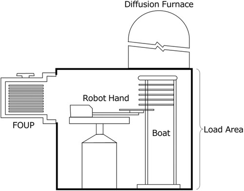
Figure 1 is a schematic diagram of the deposition equipment, which is the target in this research. Wafers are taken out from FOUP (Front-Opening Unified Pod), which is a transport container, by a robot hand and pulled into the load area. Then, the wafers are loaded into the boat and put into the diffusion furnace. Oxygen concentration in the load area must be reduced because wafer quality deteriorates by exposure to oxygen during processing. Equipment that cannot lower the oxygen concentration to the desired level is treated as anomaly and repaired. Thus, the oxygen concentration is the most important indicator of the equipment performance.

Figure 1. Schematic diagram of deposition equipment.

Semiconductor manufacturing equipment is slightly different from each other. This small difference affects the equipment performance. However, since the equipment performance can be maintained by increasing N2 pressure, it is difficult to detect anomalous equipment by monitoring only the oxygen concentration. To realize anomaly detection, it is desirable to use multiple signals. In this study, we propose a method to detect anomalous equipment from both oxygen concentration and pressure (total pressure) in the load area.

Anomaly detection method

Equipment data and the objective variable

Oxygen is excluded from the load area for quality assurance. While the deposition equipment is operated, oxygen concentration and pressure are monitored. This period is called the monitoring section. Figure 2 shows a scatter plot of oxygen concentration and pressure during the monitoring section of normal equipment and anomalous equipment.

Figure 2. Scatter plots of oxygen concentration and pressure in the monitoring section: (a) normal equipment and (b) anomalous equipment.

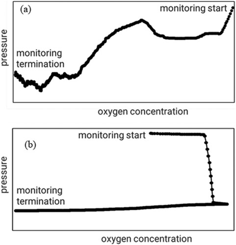
Various features were extracted from the behaviour of oxygen concentration and pressure in the monitoring section and used as explanatory variables of anomaly detection models. The goodness of the behaviour of oxygen concentration was visually evaluated by the person in charge of quality assurance, and it was used as the objective variable. Quality assurance personnel’s judgement is more accurate than computer-based judgment at least from our experience. In addition, the presence or absence of product defect is determined by the quality assurance personnel and this determination is treated as true. Figure 2(b) shows that the oxygen concentration rises once and then falls. This is difficult to detect automatically because it is necessary to judge the abnormality from the magnitude and frequency of the signal. The judgement of the abnormality depends on the experience of the quality assurance personnel, but there are no explicit criteria.

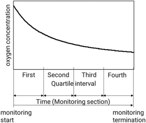
The oxygen concentration in the monitoring section of typical normal equipment is shown in Figure 3. The four divisions in the monitoring section are quartile intervals.

Figure 3. Oxygen concentration change during N2 purge.

Oxygen concentration data may contain spiked outliers. Each outlier was replaced with the mean of the values before and after the outlier.

Features

Various features can be employed for anomaly detection. In this research, considering practical applications in real manufacturing settings, features that are computationally simple and easily interpretable were selected. As a result, a total of 16 features were identified as candidates. Then, we built an anomaly detection model by combining them. In Table 1, the features are listed vertically, and the preprocessing is listed horizontally. Asterisk (*) is used to show which preprocessing was performed to calculate each feature.

Table 1. Measurements and preprocessing used for feature extraction.

	OX	PR10MA,d	OX10MA,d	PR100MA,d	PC1
F01	*	*
F02	*	*
F03	*	*
F04	*	*
F05	*	*
F06	*
F07			*
F08				*
F09			*	*
F10			*	*
F11			*	*
F12					*
F13					*
F14					*
F15					*
F16				*

A moving average of pressure (p) was calculated with 10 samples to eliminate its oscillation, and a difference of adjacent moving averages was derived. (1) $P{R}_{10MA,d}\left(k\right)=\frac{{\sum }_{i=k-1}^{k-10}{p}_i-{\sum }_{i=k}^{k-9}{p}_i}{10},$(1) where p_i is the i-th sample of p. In addition, a moving average was calculated with 10 samples to make the sum of the displacements before and after oxygen concentration (o) and pressure (PR_10MA,d) almost equal to the range of the overall signal. (2) $\begin{array}{rl}O{X}_{10MA,d}\left(k\right)& =\frac{{\sum }_{i=k-1}^{k-10}{o}_i-{\sum }_{i=k}^{k-9}{o}_i}{10},\end{array}$(2) (3) $\begin{array}{rl}P{R}_{100MA,d}\left(k\right)& =\frac{{\sum }_{i=k-1}^{k-100}{p}_i-{\sum }_{i=k}^{k-99}{p}_i}{100},\end{array}$(3) where o_i and p_i are the i-th sample of o and p.

Principal component analysis was performed on OX_10MA,d and PR_100MA,d. The score of the first principal component is PC1. The 16 features calculated from the above are explained below.

• F01: Simple regression coefficient with PR_10MA,d as an explanatory variable and OX as an objective variable.

• F02: The standard error (SE) of the predicted value of the regression line, with pressure (PR_10MA,d) as x and oxygen concentration (o) as y, was calculated using the following equation. Where $\overline{y}$ and $\overline{x}$ are the mean values of y and x, and n is the number of samples. (4) $SE=\sqrt{\begin{array}{c}{\displaystyle \frac{1}{\left(n-2\right)}}\\ \left[\sum {\left(y-\overline{y}\right)}^2-{\displaystyle \frac{{\left\{\sum \left(x-\overline{x}\right)\left(y-\overline{y}\right)\right\}}^2}{\sum {\left(x-\overline{x}\right)}^2}}\right]\end{array}}\text{.}$(4)

• F03: Correlation coefficient between PR_10MA,d and OX.

• F04: Percentage of the most frequent combination of OX and PR_10MA,d. Table 2 shows an example of the frequency of occurrence of OX and PR_10MA,d. In this equipment, the maximum value of 78 is chosen and it is divided by the total, i.e. 454.

• F05: Pressure (PR_10MA,d) at the most frequent combination in F04. For example, F05 is 50 in Table 2.

• F06: Minimum oxygen concentration in the first quartile interval.

• F07: Standard deviation of OX_10MA,d in the fourth quartile interval.

• F08: Standard deviation of PR_100MA,d in the fourth quartile interval.

• F09: Number of clusters after k-means analysis of OX_10MA,d and PR_100MA,d. The optimal number of clusters was determined by maximizing ccc (cubic clustering criteria) [6]. In the k-means cluster analysis, there is a concern that the difference in the initial value causes a difference in the clustering result. As countermeasures, k-means++[7], which reduces computational resources, and KKZ [8], which has high reproducibility, have been proposed. We used k-means++, because KKZ is more sensitive to outliers than k-means++.

• F10: The maximum ccc in F09.

• F11: Displacement of sample size in four quartile intervals, which is defined as the slope of the approximation line in Figure 4. In this figure, the vertical axis (“variable” in the figure) is the standard deviation of the number of samples belonging to 20 clusters in each quartile interval, and the horizontal axis is the quartile interval. The clusters are constructed in the space of OX_10MA,d and PR_100MA,d.

• F12: Standard deviation of PC1 in the first quartile interval.

• F13: Percent variability of PC1 in the first quartile interval, which is defined as the PC1 standard deviation in the first quartile interval divided by the PC1 standard deviation in the monitoring section.

• F14: Displacement of PC1 in four quartile intervals, which is defined as the slope of the approximation line also in Figure 4. In this figure, the vertical axis (“variable” in the figure) is the standard deviation of PC1 in each quartile interval.

• F15: Displacement of percent variability of PC1 in four quartile intervals, which is defined as the slope of the approximation line also in Figure 4. In this figure, the vertical axis (“variable” in the figure) is percent variability of PC1 in each interval, which is defined in F13.

• F16: Displacement of sample size in four quartile intervals, which is defined as the slope of the approximation line also in Figure 4. In this figure, the vertical axis (“variable” in the figure) is the standard deviation of the number of samples belonging to 20 clusters in each quartile interval. The clusters are constructed using only PR_100MA,d.

Table 3 shows the calculated features of the 16 equipment (E01 to E16), which were used to build anomaly detection models.

Figure 4. Image of displacement from the first quartile interval to the fourth quartile interval.

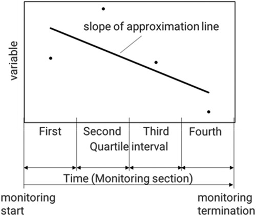
Table 2. Two-dimensional distribution table of OX and PR_10MA,d.

		OX
		3	4	5	6	7
PR10MA,d	49	0	0	0	0	0
	50	78	68	28	0	0
	51	57	59	52	61	51
	52	0	0	0	0	0

Table 3. Features calculated from data acquired from the equipment.

	F01	F02	F03	F04	F05	F06	F07	F08	F09	F10	F11	F12	F13	F14	F15	F16
E01	0.16	1.4	0.04	39.2	57	19.3	0.004	0.003	19	−22	7.9	−0.32	−0.31	1.46	1.42	4.2
E02	3.83	0.9	0.89	28.5	53	17.6	0.005	0.001	18	17.1	3.3	−0.16	−0.15	1.00	0.94	6.3
E03	2.36	4.4	0.12	19.8	47	11.2	0.005	0.004	3	−44	6.6	−0.28	−0.28	1.39	1.37	−0.1
E04	9.20	2.0	0.76	26.9	50	8.1	0.005	0.003	3	−28	4.5	−0.23	−0.20	1.46	1.26	−1.7
E05	7.31	4.3	0.44	11.0	50	10.0	0.005	0.002	6	−19	5.0	−0.17	−0.15	0.99	0.84	1.9
E06	9.13	2.2	0.90	13.6	51	11.4	0.005	0.004	15	−26	−2.7	0.01	0.01	0.84	0.81	−2.1
E07	4.84	1.4	0.92	22.5	50	7.1	0.005	0.003	20	−19	2.7	−0.16	−0.16	1.14	1.11	2.6
E08	7.71	2.1	0.84	19.4	53	14.7	0.007	0.001	18	−4.1	4.1	−0.19	−0.18	0.99	0.94	6.1
E09	10.10	3.2	0.83	16.2	56	10.3	0.005	0.004	15	−19	5.3	−0.04	−0.04	0.68	0.60	0.2
E10	8.26	2.9	0.67	35.7	53	7.3	0.005	0.003	20	−23	6.6	−0.25	−0.22	1.37	1.20	2.8
E11	5.59	1.7	0.90	17.4	46	8.9	0.005	0.003	20	−16	5.2	−0.22	−0.21	1.31	1.24	2.0
E12	7.47	2.8	0.66	20.1	52	5.7	0.004	0.006	19	−28	−0.3	−0.09	−0.08	0.96	0.86	−0.1
E13	5.70	2.9	0.78	15.7	46	12.4	0.006	0.004	15	−26	2.8	−0.22	−0.21	1.35	1.32	−1.5
E14	7.04	1.7	0.83	30.1	56	7.3	0.004	0.005	9	−38	6.0	−0.10	−0.09	1.02	0.91	0.4
E15	5.77	2.1	0.79	24.4	51	5.9	0.005	0.003	16	−18	3.9	−0.28	−0.26	1.50	1.37	0.8
E16	9.77	2.3	0.84	16.0	55	10.0	0.006	0.003	19	−35	1.7	−0.14	−0.12	1.05	0.89	1.6

Building anomaly detection models

Anomaly detection models were built with data from 16 equipment (10 normal equipment and 6 anomalous equipment). Their generalization performance was evaluated using data from 39 equipment (31 normal equipment and 8 anomalous equipment). The data for modelling and the data for performance evaluation were totally different. ROC (Receiver Operating Characteristic) curve were drawn with the logistic regression results for all explanatory variables. AUC (Area Under the Curve), which is defined as the area under the ROC curve, was calculated.

Univariate detection model

Logistic regression was performed using each of 16 features as an explanatory variable and normal or anomalous equipment as a binary objective variable.

Table 4 summarizes the results of comparing detection capabilities. F06 had the highest AUC of 0.93. This model detects anomalous equipment only from oxygen concentration.

Table 4. Comparison of AUC for univariate detection models.

feature	AUC
F06	0.93
F01	0.67
F09	0.67
F08	0.63
F16	0.61
F02	0.57
F03	0.57
F04	0.57
F14	0.57
F05	0.54
F15	0.53
F07	0.51
F12	0.50
F10	0.47
F13	0.47
F11	0.44

Multivariate detection model

The two-variable detection models were built by combining another feature with F06 selected in the single variable detection model. Table 5 summarizes the AUC of the two-variable detection models. The combination of F06 and F16 achieved the highest AUC of 1.00.

Table 5. Comparison of detection ability of models made with two features.

feature 1	feature 2	AUC
F06	F16	1.00
	F10	0.95
	F03	0.93
	F07	0.93
	F08	0.93
	F12	0.93
	F13	0.93
	F14	0.93
	F15	0.93
	F01	0.92
	F11	0.92
	F02	0.90
	F04	0.90
	F09	0.90
	F05	0.90

Since the highest AUC has already been achieved, no further evaluation is generally required. However, since the evaluation was based on limited data, we also evaluated three – and four-variable models. Three-variable detection models were built by combining F06 and F10, the combination of which achieved the second-highest AUC, with another feature. Table 6 shows the AUC. Among the three-variable detection models, the highest AUC was 0.967 for F06, F10, and F11.

Table 6. Comparison of detection ability of models made with three features.

feature 1	feature 2	feature 3	AUC
F06	F10	F11	0.967
		F01	0.950
		F03	0.950
		F07	0.950
		F08	0.950
		F12	0.950
		F13	0.950
		F14	0.950
		F15	0.950
		F05	0.933
		F02	0.933
		F09	0.933
		F04	0.917

Table 7 shows the AUC when a four-variable models were built by combining F06, F10, and F11 with another feature. Among the four-variable detection models, the highest AUC was 0.967, the same as the model with three variables.

Table 7. Comparison of detection ability of models made with four features.

feature 1	feature 2	feature 3	feature 4	AUC
F06	F10	F11	F03	0.967
			F07	0.967
			F08	0.967
			F12	0.967
			F13	0.967
			F14	0.967
			F15	0.967

Since no improvement in AUC was observed in the four-variable model, the two-variable model of F06 and F16 and the three-variable model of F06, F10, and F11 were used as multivariable detection models.

The detection model needs to detect anomalies with high accuracy even for unknown data and future data. Tables 8–10 are confusion matrices derived by applying the three models described above to the data of 39 equipment (31 normal equipment and 8 anomalous equipment).

Table 8. Anomaly detection result by a single variable model (using F06).

	Detection result OK	Detection result NG	accuracy
Quality judgment OK	29	2	82%
Quality judgment NG	5	3

Table 9. Anomaly detection result by two variables model (using F06, F16).

	Detection result OK	Detection result NG	accuracy
Quality judgment OK	29	2	82%
Quality judgment NG	5	3

Table 10. Anomaly detection result by three variables model (using F06, F10, F11).

	Detection result OK	Detection result NG	accuracy
Quality judgment OK	29	2	87%
Quality judgment NG	3	5

Discussion

We defined 16 features that represent equipment behaviour and built three models to detect anomalous equipment. At the model building stage, AUC was greater than 0.9 for all models.

As shown in Figure 2(a), both oxygen concentration and pressure tend to decrease with time under normal conditions. The equipment that was regarded as an anomaly showed a linear upward trend of oxygen concentration alone or both oxygen concentration and pressure as shown in Figure 2(b). Since such behaviour cannot be detected only by observing the oxygen concentration at the end of monitoring section, it is effective to detect it from the behaviour of the two factors, oxygen concentration and pressure, using a multivariable model.

We evaluated the ability of the detection models on the model evaluation data of 39 equipment, and the AUC was 1.000 for the combination of F06 and F16 and 0.967 for the combination of F06, F10, and F11. In addition, the detection accuracy was 82% for both the single variable model and the two-variable model while it was 87% for the three-variable model. Here, AUC is higher if the false positive rate (FPL) is lower. Therefore, predictive accuracy does not necessarily equate to AUC.

There were no significant differences between the single variable and multivariable methods in the present evaluation data. If the behaviour of the equipment changes, and this is a change in the relationship between the variables, a multivariable-model method will be beneficial. Therefore, the results demonstrate that detecting anomalous equipment from the behaviour of two factors, oxygen concentration and pressure, contributes to performance improvement.

By jointly using three models, the person in charge of quality assurance can determine whether further inspection is needed or not.

To further improve the detection performance, more data needs to be accumulated.

Conclusion

In this study, we developed anomaly detection models for semiconductor processing equipment. We extracted 16 types of features from the behaviour of oxygen concentration and pressure in the load area, and built univariate and multivariate models combining these features to improve the ability to detect anomalous equipment. These models were able to detect anomalous equipment that could not be detected by monitoring only the oxygen concentration.

This study focused on the loading area, and anomalous equipment can be detected before the full assembly. If equipment is judged to be anomaly (NG) after the full assembly without the developed detection model, the equipment needs to be disassembled to adjust the equipment. As a result, it becomes possible to greatly shorten the adjustment time, which contributes to shortening the processing lead time.

In the future, it is expected that the performance required for equipment will further increase as the design rules for semiconductor devices evolve. We will be required to rearrange features and build high-performance anomaly detection models repeatedly.

Acknowledgments

We would like to thank the engineers of KOKUSAI ELECTRIC CORPORATION for their cooperation in this research.

Disclosure statement

No potential conflict of interest was reported by the author(s).

References

- Okada M, Haga Y. Wafer warpage classification adapted to pragmatic equipment operation. AEC/APC Symposium Asia. 2019.
- Hirai T, Kano M. Adaptive virtual metrology design for semiconductor Dry etching process through locally weighted partial least squares. IEEE Trans Semicond Manuf. 2015;28(2):137–144. doi:10.1109/TSM.2015.2409299
- Kano M, Nakagawa Y. Data-based process monitoring process control and quality improvement: recent developments and applications in steel industry. Comput Chem Eng. 2008 Jan-Feb;32(1-2):12–24. doi:10.1016/j.compchemeng.2007.07.005
- Kano M, Hasebe S, Hashimoto I, et al. Evolution of multivariate statistical process control: application of independent component analysis and external analysis. Comput Chem Eng. 2004 Apr;28(6-7):1157–1166. doi:10.1016/j.compchemeng.2003.09.011
- Hirai T, Ito N, Kano M. Identifying causal factors by mean-value replacement contribution. J Soc Instrum Control Eng. 2021;57(2):86–91.
- SAS (R) Technical Report A-108: Cubic Clustering Criterion. SAS Inst Paperback in English. 1992.
- Arthur D. k-means++: The advantages of careful seeding. Proc. of the Eighteenth Annual ACM-SIAM Symposium on Discrete Algorithm. 2007;1027-1035.
- Katsavounidis I, Kuo CCJ, Zhang Z. A New initialization technique for generalized lloyd iteration. IEEE Signal Process Lett. 1994 Oct;1(10):144–146. doi:10.1109/97.329844