Estimating the Importance of Families in Modeling Educational Achievement Using Linked Swedish Administrative Data

Abstract

While the family is a critical determinant of educational achievement, methodological difficulties and the availability of data limit estimation of the family contribution in school effectiveness models. This study uses multilevel modeling to estimate the proportion of variation in student educational achievement between families, family-level intraclass correlation coefficients, and specific family structure effects (family size, birth order, birth spacing, sibling sex ratio). We use cross-classified random effects to account for school and neighborhood variation. We analyze Swedish administrative education records linked with birth records for four academic cohorts of students, with siblings identified from a wider pool of 21 cohorts. We show that almost half of the variation in student achievement described as “between students” in traditional school effectiveness studies would be better described as variation “between families,” suggesting effectiveness research might give greater consideration to family-based interventions in tandem with existing student- and school-based approaches to raising low achievement.

Keywords:

• Educational attainment
• educational achievement
• family clusters
• family structure
• school clusters
• neighborhood clusters
• multilevel modelling
• hierarchical linear modelling

Introduction

When studying the factors associated with student educational achievement, it is important to model the different contexts in which children are educated and raised, such as schools, families, and neighborhoods. Early school effectiveness research naturally focused on the influence of schools (Goldstein, 2011; Teddlie & Reynolds, 2000). Typical studies would fit two-level multilevel models (i.e., hierarchical linear, mixed-effects or random effects models; Bryk & Raudenbush, 2002; Goldstein, 2011; Snijders & Bosker, 2012) to partition the variation in achievement into variation between schools and variation between students (Aitkin & Longford, 1986; Goldstein, 1997; Raudenbush & Willms, 1995). Studies using these approaches often refer to the between-school variation in achievement as that part “explained by schools” or “attributable to schools”; however, we avoid such language here due to the risk of implying causal effects, the limitations to causal interpretations are explained further in Section “Model Assumptions”.

Many extensions to school effectiveness models have been developed, including modifications to study additional sources of variation in student achievement. These include three-level models to account for the location of schools within school districts or other geographic regions (Gandhi et al., 2018), teachers (Nye et al., 2004), and academic cohorts within schools (Willms & Raudenbush, 1989), and cross-classified models to account for the neighborhoods within which students reside (Garner & Raudenbush, 1991; Leckie, 2009; Raudenbush, 1993). The family is another important source of variation in student achievement and potential level at which effectiveness researchers might intervene to raise student achievement.

Educational effectiveness studies attempting to quantify the effects of an intervention may adjust for family characteristics such as household socioeconomic status or parent education measures. However, the measures available are limited by the data collection, and these may not encapsulate all relevant factors, particularly for more complex interventions or interventions with more diverse outcomes. Modeling the between-family variation captures a broad holistic conceptualization of family variation, but as for schools, this should not be interpreted as all the variation “explained” by families.

Including between-family effects in the modeling can be combined with specific family-level measures such as family structure or socioeconomic status to quantify the proportion of between-family variation accounted for by observed family characteristics. Further, where interventions are targeted directly at the family level, such as conditional cash transfers (Berg et al., 2013), one can directly ascertain the degree to which this reduces variability between-families. This is especially important when family-level interventions are related to school contexts, such as improving teacher-parent communication (Kraft & Dougherty, 2013), since isolating the between-family vs. between school/classroom effects allows a clearer insight into in which domain the intervention is operating. Where interventions directly overlap between clusters, such as those aimed at schools and families, a multilevel approach can simultaneously accommodate multiple types of clusters and the characteristics of each of these clusters (Kelcey et al., 2020; Stallasch et al., 2021). Finally, modeling the between-family variation also acknowledges family-level residual clustering; this is important when the aim is to make inferences about family-level interventions and characteristics as these would otherwise be estimated with spurious precision (Type I errors of inference).

Though studies commonly adjust for observed family characteristics such as socioeconomic status on achievement or the proportion of variance in achievement that is between families, there are few which have been able to simultaneously study the role of school and families in their analyses (Downey & Condron, 2016). A notable exception is Rasbash et al. (2010), who study the relative importance of families as a source of variation in student end-of-compulsory-schooling General Certificate of Secondary Education (GCSE; age 16) examination scores in England in 2007. However, they were only able to identify twin families: students were assumed to be twins if they shared the same date of birth and postal address; they were not able to identify other family types. Thus, their reported finding that 40% of the variation in student progress during secondary schooling lies between families might be considered as an “upper bound” as to the importance of families in their study. The current paper aims to estimate the role of families in models of student achievement and school effectiveness using richer Swedish data, which allows a broader identification of families. We analyze administrative data on four consecutive academic cohorts (2006–2009) of secondary school students in Sweden as they reach the end of compulsory schooling (age 16). The data include information on student achievement, schools attended, and neighborhoods of domicile. The data also report the genetic relations between students allowing us to identify not just twin families but families comprised of full and half-siblings. We carry out three sets of analyses on these data. First, we apply a restricted definition of families as twin pairs similar to Rasbash et al. (2010). Second, we apply the broader definition of families made possible by the current data. We then contrast these two sets of results to demonstrate how decisions regarding the definition and operationalization of families in school effectiveness models can lead to substantively very different conclusions as to the relative importance of families in modeling student achievement. We also present school-, family-, and neighborhood-level intraclass correlations coefficients (ICCs) to facilitate comparisons to studies reporting correlation-based approaches and inform statistical power calculations for experiments, especially those that randomize families. Third, we explore the associations between student achievement and four measures of family structure: family size, birth order, birth spacing, and sibling sex composition.

Background: Literature and Conceptual Framework for Understanding Family Effects on Student Achievement

Conceptual Framework for Evaluating the Effect of Clustering on Student Achievement

There has been a move to introduce market forces in education to induce competition between schools to improve student outcomes in many countries. In Sweden, this process began in the 1990s, including decentralizing school finance, a voucher system to enable parental choice, and funding private schools (Björklund et al., 2003). In response to these policy changes, there is a demand to understand how attempts at increasing overall student achievement have also driven inequality of opportunity. Therefore, it is of increasing policy relevance to model the variation in achievement associated with the characteristics and groupings of each child, including the variation in achievement that lies between families (Böhlmark & Holmlund, 2011; Holmlund et al., 2014; Skolverket, 2018).

Drivers of variation in achievement between children may stem from early differences in genetic endowments and the characteristics of pre-natal and neo-natal environments (Björklund & Jäntti, 2012). As children develop, the characteristics of early home environments, including the resources available through measures such as household income, will continue to impact their future achievement through mechanisms such as the number of books in the home (Björklund et al., 2003). The capacity of parents to support a child’s education will, in turn, be related to their own education and softer measures such as their motivation and commitment to education manifested through actions such as time spent reading to children (Holmlund et al., 2014). Aspects of household composition also contribute to variation in achievement, including the number and age profile of siblings who may provide academic support or the presence of older household members such as grandparents who may provide childcare (Skolverket, 2018). Wider environments such as the neighborhoods in which a child lives may directly influence cognition or sleep through pollution and noise, or provide access to additional educational resources such as libraries and green spaces (Lindahl, 2011). Schools directly affect achievement through resources and teacher quality, in addition to exogenous characteristics such as the ability of peers (Böhlmark & Holmlund, 2011).

A natural approach to studying the importance of families in studies of student and school achievement is to specify a model which includes as many of these family-level characteristics as possible (as well as measures of the child, their environments, and schools). However, sound interpretation of the conditional estimates requires (i) a more nuanced selection of the measures to include or omit; (ii) a recognition of the effect of the many characteristics that are not (or cannot) be measured; and (iii) the assumptions of how these characteristics interact. This paper provides an important starting point for this type of analysis by providing estimates of the overall importance of family units in modeling variance in student achievement. Therefore, our primary focus is on estimating and partitioning variance at the family level rather than causal attribution of a family effect per se.

Evaluating How Family Units Are Associated With Student Achievement

Though school effects are of principal interest in school effectiveness research, the importance of other social contexts such as the neighborhoods in which students live are increasingly being recognized. We propose that family effects, typically argued to represent a combination of genetic and family environmental factors, should also be accounted for by school effectiveness researchers. While researchers frequently adjust for specific family characteristics such as socioeconomic status in their models (e.g., Leckie & Goldstein, 2009), this approach does not lead to a measure of the unexplained variation in the outcome, which is common to all siblings in a family regardless of the underlying factors causing the differences. Estimating the overall proportion of variance that is between families may provide useful evidence for triallists and policymakers in understanding how to raise achievement. By extending standard school effectiveness models to include a family random effect as well as the usual school random effect, we can attempt to quantify the relative importance of families as a general source of variation in student achievement (Rasbash et al., 2010).

An early approach for identifying the importance of families was to simply estimate correlations between children within a family (Hauser & Featherman, 1976), and therefore typically the same school and neighborhood, and then contrast these with estimated correlations between unrelated children from the same school or neighborhood. For example, Solon et al. (2000) use the US Panel Study of Income Dynamics to compare individuals in terms of years of schooling. They find a sibling correlation of 0.5 (same family and same neighborhood) and a neighbor correlation of 0.2 (different families, but same neighborhood) and attribute the difference between these correlations to the family: families account for 30% of the variation in years of schooling. This approach can be extended when the sibling type (full sibling, half-sibling, twin) is known, allowing one to identify how the sibling correlation strengthens as a function of genetic relatedness (Koeppen-Schomerus et al., 2003). This approach can also be reformulated as a multilevel model, with a random effect for each set of siblings within the same family with the same type of genetic relatedness (Guo & Wang, 2002; Lindahl, 2011; Mazumder, 2008; Nicoletti & Rabe, 2013), though these are restrictive in terms of accounting for other contexts and estimating the overall family effect. One can use a more conventional definition of family within a multilevel model to identify an overall family effect (Bu, 2014), and Rabe-Hesketh et al. (2008) extend this approach to explore broader definitions of family, modeling siblings as nested within “immediate families” and within “wider families” and thereby allowing for correlated outcomes between cousins.

Evaluating How Family Variables Are Associated With Student Achievement

Having established the relative importance of families as a general source of variation in student achievement, attention might then shift to exploring how specific family characteristics account for the within- and between-family variation in student achievement. These include socioeconomic status (e.g., the number of books in the household, parental education, occupation, or income), demographic factors (e.g., mother’s age at birth), and social factors (e.g., marital status or whether both parents are living in the household) (Björklund et al., 2010; Bredtmann & Smith, 2018; Eriksson et al., 2016). In this study, we focus on family characteristics relating to the structure of the family. We focus on four aspects of family structure available in our Swedish administrative data: family size, birth order, birth spacing, and sibling sex composition.

Family size is hypothesized to operate on student achievement in several ways. The “resource dilution model” (Blake, 1981) describes how diminishing resources are shared across increasing numbers of children in larger families, leading to a tradeoff between the quantity of children and quality of child outcomes. The “confluence model” (Zajonc & Bargh, 1980) describes how patterns of socialization, and consequently cognitive development, are negatively influenced by increasing family size. Family size is also related to other demographic processes, including increasing postponement of childbearing and consequently smaller families associated with higher levels of education among mothers and better outcomes for children (Joshi, 2002; Kneale & Joshi, 2008). Empirical studies have tended to show a negative association between family size and educational achievement (Dundas et al., 2014; Iacovou, 2008; Kuo & Hauser, 1997).

Birth order operates as an individual-level family structure variable (as opposed to family-level structure variables, which apply equally across the whole sibship). Birth order can provide an indicator of the context of the individual child within the family and has been hypothesized to signal differences in the range and type of resources that may be allocated (Booth & Kee, 2009). Birth order may also indicate potential individual characteristics, as hypothesized in optimal stopping theory, where parents may stop having children after a difficult child (Lundberg & Svaleryd, 2017). In researching birth order effects, early empirical studies simply compared individuals with differing birth orders across families, confounding within- and between-family effects of birth order on the studied outcomes. This is problematic since children of higher birth orders are, on average, from larger and worse-off families in terms of unobserved characteristics associated with individual outcomes. This was formalized as the “admixture” hypothesis (Page & Grandon, 1979) and is contrasted with the confluence and resource dilution models (Sandberg & Rafail, 2014). Studies that successfully differentiate the within- and between-family effects of birth order show the within effect to be smaller, but still negative (Booth & Kee, 2009; Iacovou, 2008)or no longer significant at all (Rodgers et al., 2000; Wichman et al., 2006). Such approaches have rarely been applied to the Swedish data, an exception being Lindquist et al. (2016), who use this approach for modeling entrepreneurship, contrasting outcomes for firstborn children with other birth orders.

Birth spacing is typically characterized by age differences between sibling pairs (as this is the unit for comparison through correlation) rather than the spacing across all siblings within a family. The mechanisms through which birth spacing influences educational achievement overlap with those discussed for family size. Zajonc (1976) suggests that wider birth spacing leads to less resource dilution. Alternatively, there may also be positive complementarities associated with closer birth spacing, such as greater economies of scale (Buckles & Munnich, 2012; Pettersson-Lidbom & Skogman Thoursie, 2009; Zajonc, 1976) and lower opportunity costs for mothers (e.g., less time out of the labor market).

Sibling sex composition is typically concerned with the family proportion of male siblings or the presence of a male sibling within the sibship. Empirical studies for student achievement have found positive effects of having male siblings on girls’ educational achievement (Bound et al., 1986; Butcher & Case, 1994). In addition, families with a male child are more likely to consider saving for all their children’s college education; thus, having a male sibling increases the chances of a female getting financial support for further education (Powell & Steelman, 1989). However, this mechanism has likely declined in salience in recent decades with the shift to greater gender equality.

Data

We analyze Swedish student administrative data on four academic cohorts of children who finished compulsory schooling (age 16) in Sweden between 2006 and 2009. The sample consists of 357,459 students nested in 1,298 secondary schools, 5,998 neighborhoods (defined at the small area market statistics level), and 301,090 families (defined below), of which 53,754 families have more than one child in the dataset between 2006 and 2009. Table 1 reports descriptive statistics for this sample.

Table 1. Descriptive statistics for child and family characteristics.

	Student (n = 357,459)
Child-level continuous variables	Mean	SD
Student achievement (standardized)^a	0.293	0.979
Age within year in months (centered on July)	0.759	3.344
Child-level categorical variables	Count	Percent
Female	174,240	48.7
Immigrant status: Swedish (no recent immigration history)	340,156	95.2
Immigrant status: 1st generation (child born outside Nordic countries)	12,639	3.6
Immigrant status: 2nd generation (at least 1 parent born outside Nordic countries)	4,610	1.3
Cohort: finish compulsory schooling in 2006	92,880	26.0
Cohort: finish compulsory schooling in 2007	91,182	25.5
Cohort: finish compulsory schooling in 2008	89,072	24.9
Cohort: finish compulsory schooling in 2009	84,325	23.6
Family structure variables (N = child)	Count	Percent
Birth order: 1st born child	150,693	42.2
Birth order: 2nd born child	127,618	35.7
Birth order: 3rd born child	55,468	15.5
Birth order: 4th born child	16,569	4.6
Birth order: 5th born child	4,650	1.3
Birth order: 6th (or more) born child	2,461	0.7
Family size: Children from a 1-child family	22,531	6.3
Family size: Children from a 2-child family	157,876	44.2
Family size: Children from a 3-child family	114,471	32.0
Family size: Children from a 4-child family	41,161	11.5
Family size: Children from a 5-child family	13,261	3.7
Family size: Children from a 6 (or more) child family	8,159	2.3
Birth spacing: Child from family with zero spacing	25,006	7.0
Birth spacing: Child from close-spaced family (1–24 months)	46,002	12.9
Birth spacing: Child from wide-spaced family (>24 months)	286,451	80.1
Child from mixed-gender sibships	222,132	62.1
	Family (n = 301,980)
Family structure variables (N = families)	Count	Percent
Family size: Number of 1 child families	22,531	7.5
Family size: Number of 2 child families	135,846	45.0
Family size: Number of 3 child families	94,488	31.3
Family size: Number of 4 child families	32,754	10.8
Family size: Number of 5 child families	10,312	3.4
Family size: Number of 6 (or more) child families	6,049	3.4
Birth spacing: Number of families with zero spacing	23,780	7.9
Birth spacing: Number of families with close spacing (1–24 months)	33,117	11.0
Birth spacing: Number of families with wide spacing (>24 months)	245,083	81.1
Number of families with mixed-gender sibships	184,116	61.0

Note. ^aStudent achievement is standardized to have zero mean and variance of one.

Our measure of student achievement is based on national tests taken at the end of compulsory schooling across a wide range of subjects. A score of 0, 10, 15, or 20 is awarded for each subject. Scores are then summed across the student’s best 16 subjects to produce a total achievement score (0–320 points). We cannot adjust for the number of subjects (capped at 16) or different subject choices; however, we note that such averages are commonly used to proxy achievement in academic research and policy evaluation (Department for Education, 2019; Goldstein, 1997).

We define families to be children with the same biological mother. Thus, siblings in our families include not just twins but full siblings and maternal half-siblings, based on the assumption that children are most likely to remain with their mother should their parents separate. Among our sample, 44% of children are from one-child families, 32% from two-child families, and 21% from larger families (three or more children). This compares with OECD estimates of 39%, 46%, and 15% for Sweden using data from 2015 (OECD, 2016). We note that Sweden’s demographics are comparable to other countries, with figures of 44%, 40%, and 16% for the UK, 42%, 36%, and 22% for the US, and 45%, 39%, and 16% for all OECD countries. Likewise, while school systems differ between countries, those of Sweden, the UK, and the US are broadly comparable, with similar scores on the equality of opportunity (the index of student economic, social, and cultural status) calculated using PISA data (Benito et al., 2014).

Having defined the families in the data, we then derive the four measures of family structure from the sample data: family size, birth order, birth spacing, and sibling sex composition. These family-level measures are defined using not just the four analysis cohorts (2006–2009) but additionally 17 earlier cohorts (1988–2005). We do this to capture as accurately as possible the family structure relevant to the analysis cohorts.

Family size refers to the number of children per family, including maternal half-siblings. This is an important control for identifying the effect of birth order (since birth order is constrained by family size) to the extent that some studies estimate birth order regressions separately for each family size (e.g., Black et al., 2011). However, we estimate a single model with both birth order and family size entered as covariates for simplicity. Both family size and birth order can be entered as continuous variables (e.g., Kanazawa, 2012) and interpreted as linear effects. However, we specify both family size and birth order as categorical variables ranging from first/one child categories to sixth/six child categories as the highest category to allow for potential non-linearity of effects. We note that it would be possible to include interactions between family size and birth order to explore non-additivity of effects (Wichman et al., 2006), but we do not pursue this here for simplicity.

Birth order refers to the order a child is born accounting for siblings across all 21 cohorts of data (1988–2009). We allow ties in ranking, and so, for example, a pair of firstborn twins would both be assigned a birth order of one, and a subsequent sibling would be assigned a birth order of three. Birth order is also entered as a categorical variable, where we specify firstborn children as the reference category.

Birth spacing is defined as the difference between the first and last birth date within the family. We do not enter this into our models as a continuous measure because there is a discontinuity between families with zero spacing (singleton, twin, or triplet only families) and nine months (families with siblings from multiple pregnancies). Furthermore, the effect beyond nine months is likely to be non-linear. Instead, we follow Powell and Steelman (1993) in using 2 years as the threshold between “close” and “wide” spacing. We thus have a three-category measure of family spacing, with zero spacing as the reference category, spacing of 2 years or less (but greater than zero), and spacing of more than 2 years.

Sibling sex composition is operationalized as a dichotomous variable for mixed-gender families compared with single-sex families (Bu, 2014).

We observe several other student-level characteristics, including gender, date of birth, and immigration history. We use the date of birth to construct each student’s “age within an academic year.” We measure this variable in months and center it on the middle of the academic year. . Immigration history distinguishes children as first-generation immigrants (child born outside Nordic countries), second-generation immigrants (one or both parents born outside Nordic countries), or Swedish (no recent immigration history).

A particularly important variable not available in these data was student prior achievement when they entered their secondary schools. Therefore, our models are potentially inadequate with respect to adjusting for school differences in the academic composition of students (Goldstein, 1997), a point that we shall return to in the discussion. Though we cannot investigate the impact of omitting this variable in our analyses of the Swedish data, in our supplementary materials we explore the impact of accounting for prior achievement on the estimates of between-family variance through exploring data on English students and recreating models analogous to Rasbash et al. (2010) that do and do not account for prior achievement.

Methods

In this section, we describe what shall refer to as the “single-cohort twins” approach and contrast it with the preferred “multiple-cohort siblings” approach. For each approach, we present four models of student achievement of increasing complexity to highlight the contribution of schools, families, and person- and family-level characteristics.

Single-Cohort Twins Approach Models

The “single-cohort twins” approach uses the twins-based definition of family employed by Rasbash et al. (2010). Let $y_{i\left(j,k,l\right)}$ denote the achievement of student $i$ ($i=1,\dots ,N$) in school $j$ ($j=1,\dots ,J$) in family $k$ ($k=1,\dots ,K$), and neighborhood $l$ ($l=1,\dots ,L$). Let $d_k$ denote a dummy variable for whether family $k$ is a twin-family. Note that while students are separately nested within schools, families, and neighborhoods, the three contexts are crossed-classified with one another (Leckie, 2013; Stephen W Raudenbush & Bryk, 2002), for example, not all children from the same neighborhood attend the same school and vice versa.

Model 1.1 is a two-level students-within-schools model. The model can be written as (1.1) $${\mathit{y}}_{\mathit{i}}={\mathit{\beta }}_0+{\mathit{\beta }}_1{\mathit{d}}_{\mathit{k}}+{\mathit{s}}_{\mathit{j}}+{\mathit{e}}_{\mathit{i}},$$(1.1) where $s_j$ and $e_i$ denote the school and student random effects respectively; each assumed normally distributed with zero means and constant variances, $s_j\sim N\left(0,{\sigma }_s^2\right)$ and $e_i\sim N\left(0,{\sigma }_e^2\right)$ respectively.

Model 1.2 is a two-level students-within-families model. The model can be written as (1.2) $${\mathit{y}}_{\mathit{i}}={\mathit{\beta }}_0+{\mathit{\beta }}_1{\mathit{d}}_{\mathit{k}}+\left({\mathit{f}}_{\mathit{k}}+{\mathit{e}}_{\mathit{i}}\right){\mathit{d}}_{\mathit{k}}+{\mathit{u}}_{\mathit{i}}\left(1-{\mathit{d}}_{\mathit{k}}\right),$$(1.2) where $f_k$ and $e_i$ denote the family and student random effects for twin-families and $u_i$ denotes the single combined family and individual random effect for singletons. The random effects are assumed normally distributed with zero means and constant variances, $f_k\sim N\left(0,{\sigma }_f^2\right)$ and $e_i\sim N\left(0,{\sigma }_e^2\right)$ and $u_i\sim N\left(0,{\sigma }_u^2\right)$ respectively.

Model 1.3 is a three-way school-by-family-by-neighborhood cross-classified model which incorporates the school and family random effects of the previous two models and additionally adjusts for neighborhood. The model can be written as (1.3) $${\mathit{y}}_{\mathit{i}}={\mathit{\beta }}_0+{\mathit{\beta }}_1{\mathit{d}}_{\mathit{k}}+{\mathit{s}}_{\mathit{j}}+{\mathit{n}}_{\mathit{l}}+\left({\mathit{f}}_{\mathit{k}}+{\mathit{e}}_{\mathit{i}}\right){\mathit{d}}_{\mathit{k}}+{\mathit{u}}_{\mathit{i}}\left(1-{\mathit{d}}_{\mathit{k}}\right),$$(1.3) where $n_l$ denote the neighborhood random effects, $n_l\sim N\left(0,{\sigma }_n^2\right),$ and all other terms are defined as before.

Finally, model 1.4 extends model 1.3 by including additional covariates such as student age and gender. The model can be written as (1.4) $${\mathit{y}}_{\mathit{i}}={\mathit{\beta }}_0+{\mathit{\beta }}_1{\mathit{d}}_{\mathit{k}}+{\mathbf{x}}_{\mathit{i}}^{\mathrm{\prime }}\mathbf{\gamma }+{\mathit{s}}_{\mathit{j}}+{\mathit{n}}_{\mathit{l}}+\left({\mathit{f}}_{\mathit{k}}+{\mathit{e}}_{\mathit{i}}\right){\mathit{d}}_{\mathit{k}}+{\mathit{u}}_{\mathit{i}}\left(1-{\mathit{d}}_{\mathit{k}}\right),$$(1.4) where ${\mathit{x}}_i$ denotes the vector of additional covariates and $\mathbf{\gamma }$ the associated vector of regression coefficients.

Multiple-Cohort Siblings Approach Models

We observe four cohorts of students in the Swedish data and can identify families with siblings as well as twins. We, therefore, adjust models 1.1, 1.2, 1.3, and 1.4 to account for the features of our data. We denote the resulting models: 2.1, 2.2, 2.3, and 2.4. Specifically, we include cohort dummy variables in each of these new models to allow for any change in average student achievement over time. We also remove the twin dummy variable from the models to shift the focus to families in general, rather than just twin-families.

Model 2.1 (c.f., model 1.1), the two-level students-within-schools model, is written as (2.1) $${\mathit{y}}_{\mathit{i}}={\mathit{\beta }}_0+{\mathit{\beta }}_1{2007}_{\mathit{i}}+{\mathit{\beta }}_2{2008}_{\mathit{i}}+{\mathit{\beta }}_3{2009}_{\mathit{i}}+{\mathit{s}}_{\mathit{j}}+{\mathit{e}}_{\mathit{i}},$$(2.1) where ${2007}_i,$ ${2008}_i$ and ${2009}_i$ denote year dummies, with 2006 being the omitted category.

Model 2.2 (c.f., model 1.2), the two-level students-within-families model, is written as (2.2) $${\mathit{y}}_{\mathit{i}}={\mathit{\beta }}_0+{\mathit{\beta }}_1{2007}_{\mathit{i}}+{\mathit{\beta }}_2{2008}_{\mathit{i}}+{\mathit{\beta }}_3{2009}_{\mathit{i}}+{\mathit{f}}_{\mathit{k}}+{\mathit{e}}_{\mathit{i}},$$(2.2) where we now make no distinction between twin-families and other families.

Model 2.3 (c.f., model 1.3) combines the students-within-schools and students-within-families models and additionally adjusts for neighborhood influences. (2.3) $${\mathit{y}}_{\mathit{i}}={\mathit{\beta }}_0+{\mathit{\beta }}_1{2007}_{\mathit{i}}+{\mathit{\beta }}_2{2008}_{\mathit{i}}+{\mathit{\beta }}_3{2009}_{\mathit{i}}+{\mathit{s}}_{\mathit{j}}+{\mathit{n}}_{\mathit{l}}+{\mathit{f}}_{\mathit{k}}+{\mathit{e}}_{\mathit{i}},$$(2.3)

Model 2.4 (c.f., model 1.4) extends model 2.3 by adding in additional covariates $x_i.$ (2.4) $${\mathit{y}}_{\mathit{i}}={\mathit{\beta }}_0+{\mathit{\beta }}_1{2007}_{\mathit{i}}+{\mathit{\beta }}_2{2008}_{\mathit{i}}+{\mathit{\beta }}_3{2009}_{\mathit{i}}+{\mathbf{x}}_{\mathit{i}}^{\mathrm{\prime }}\mathbf{\gamma }+{\mathit{s}}_{\mathit{j}}+{\mathit{n}}_{\mathit{l}}+{\mathit{f}}_{\mathit{k}}+{\mathit{e}}_{\mathit{i}},$$(2.4)

In addition to the covariates for model 1.4 described above, model 2.4 includes immigrant status, family size, birth order, birth spacing, and sibling sex composition.

Estimation

We fit all models using the Markov chain Monte Carlo (MCMC) computational procedure as implemented in the MLwiN software (Browne, 2020; Charlton et al., 2020). We use MCMC as maximum likelihood estimation proved computationally prohibitive given the cross-classified nature of the multilevel models combined with the size of the data. We call MLwiN from within Stata (StataCorp, 2021) using the runmlwin command (Leckie & Charlton, 2012). Starting values for all parameters are obtained from simpler models estimated using maximum likelihood estimation (Goldstein, 1986) again in MLwiN. We specify minimally informative (diffuse, vague, or flat) priors for all parameters. We use the MLwiN default inverse gamma priors for the variance components. We note that results are somewhat sensitive to the choice of priors, with uniform priors tending to give slightly larger variance estimates than the default priors. As expected, this is more pronounced for the family variance component because the family clusters are small (Browne & Draper, 2006). We estimate the twins approach models with a burn-in of 50,000 iterations and a monitoring chain of 500,000 iterations, and the siblings approach models with a burn-in of 500 iterations and a monitoring chain of 5,000 iterations. The extreme definition of families in the “twin-family” models required the MCMC sampler to be run for considerably longer than would typically be the case (see Rasbash et al. (2010) for further discussion). Visual assessments of the parameter chains and standard MCMC convergence diagnostics suggest that these periods are sufficiently long to generate robust parameter summaries. The effective sample size for each parameter chain exceeded 250. Annotated code for the models is provided in the supplementary materials.

When we report the results, we present the means and standard deviations (SDs) of the parameter chains for each parameter. These quantities are analogous to parameter estimates and standard errors obtained in frequentist analyses. We use the Bayesian deviance information criterion (DIC) to compare model fit (Spiegelhalter et al., 2002). Smaller DIC values are preferable, and a reduction of five or more points between models is considered substantial (Lunn et al., 2012).

Model Assumptions

Like all regression models, multilevel models make particular assumptions that must be borne in mind when interpreting the results. Especially relevant to our work, multilevel models assume the cluster random effects and covariates are independent (e.g., school effects are independent of control variables such as prior achievement), that the clusters random effects are independent within each level (e.g., the effect of one school is independent of the effect of neighboring schools), and that the cluster random effects are independent across levels (e.g., school effects are independent of the effects of the neighborhood in which the child lives).

The assumption of independence between cluster random effects and covariates is perhaps the most important. With respect to school clustering for example, more effective schools may attract more motivated students; thus, while we might see a large school effect due to good school practice, some element of this effect will potentially reflect selection of more motivated students into more effective schools (Castellano et al., 2014; Raudenbush & Willms, 1995). To the extent to which this is true, the estimated school effects represent a mix of selection (composition and contextual) as well as causal effects (policy and practice) of schools. Likewise, families with higher incomes tend to have children with other advantages. The estimated family effects will be composed partly of the causal effects of family practice, but also factors correlated with household income. In both examples above the selection is positive, making it likely the cluster effects are overstated, reflecting a confounding of causal cluster effects and selection effects. It is also possible for the selection to run in the other direction, for example, low-performing schools would typically attract additional funding, which one would typically expect to be positively correlated with achievement.

The assumption of independence across clusters is also a potential concern. We might reasonably expect sorting of families into schools and neighborhoods, and this sorting is likely to have a common direction, i.e., where we define “better” as a propensity for higher achievement, then “better” families prefer to live in “better” neighborhoods close to “better” schools. For interpretation, we therefore make statements as to the variation in school means versus the variation in neighborhood means, where these means again represent complex mixtures of selection and causal effects that cannot be separated. With multiple clusters, we must take care with which covariates to include, and their interpretation. A relevant example for this study is controlling for prior achievement. When estimating school effects alone, it is common to control for prior achievement so that we estimate student progress while attending the school. However, in a model which also includes family clustering, which would have directly impacted on prior achievement, we could remove some of the family input which we would have hoped to attribute to the family unit.

Despite these difficulties in satisfying the model’s assumptions, this analysis remains important for evaluating interventions. In the present paper, the primary focus is on estimating and partitioning variance in student achievement at the family level rather than causal attribution of a family effect per se. That is, our results are descriptive quantification of inequalities between families, schools, and neighborhoods in the education system, which are of interest in their own right. We view these results as an informative stepping stone to more ambitious future causal analyses of interventions that might start to tease apart causal versus selection effects at each level.

Results

We present our results in three parts. Section “Single-Cohort Twins Approach Models Fitted to the Sweden 2007 Data” describes the estimates from the “single-cohort twins” approach models (models 1.1–1.4) fitted to the 2007 cohort of Swedish students. Section “Multiple-Cohort Siblings Approach Models Fitted to the Sweden 2006–2009 Data” describes the estimates from the four “multiple-cohort siblings” approach models (models 2.1–2.4) fitted to the 2006–2009 cohorts of Swedish students. Comparing these with the “single-cohort twins” approach models (models 1.1–1.4) shows the effects of change in family definition from twin families to families with multiple sibship types. As indicated in Section “Model Assumptions,” our models are associational rather than causal, providing descriptive estimates of the observed covariate and cluster effects.

Single-Cohort Twins Approach Models Fitted to the Sweden 2007 Data

Table 2 presents results for the single-cohort twins approach models 1.1, 1.2, 1.3, and 1.4 (see Section “Single-Cohort Twins Approach Models”) fitted to the 2007 cohort of Swedish students. In addition to the usual regression coefficients and estimated variance components, we report both the total variance (the sum of the estimated variance components for students in twin families) and the variance partition coefficients (the proportion of the total variation which is between each level of analysis: students, schools, families, and neighborhoods).

Table 2. Single-cohort twins approach models fitted to the Sweden 2007 data.

Parameter	Model 1.1		Model 1.2		Model 1.3		Model 1.4
	Est.	SE	Est.	SE	Est.	SE	Est.	SE
Regression coefficients
Intercept	−0.002	(0.009)	0.006*	(0.003)	−0.003	(0.009)	−0.190***	(0.010)
Twin-family	0.071***	(0.021)	0.069*	(0.027)	0.062*	(0.025)	0.055*	(0.025)
Age within year (months)							0.012***	(0.001)
Female							0.369***	(0.006)
Variance components
School	0.083***	(0.004)			0.070***	(0.004)	0.069***	(0.004)
Neighborhood					0.038***	(0.002)	0.039***	(0.002)
Family (twins only)			0.575***	(0.033)	0.477***	(0.030)	0.476***	(0.029)
Student (twins only)			0.290***	(0.013)	0.289***	(0.013)	0.268***	(0.012)
Family + Student (non-twins only)			0.917***	(0.004)	0.812***	(0.004)	0.777***	(0.004)
Student	0.839***	(0.004)
Total	0.922		0.865		0.874		0.852
Variance partition coefficients (VPCs)^a
School	9%				8%		8%
Neighborhood					4%	5%
Family			67%		55%		56%
Student	91%		33%		33%		31%
Model summary
Number of schools	1,152				1,152		1,152
Number of neighborhoods					4,747		4,747
Number of non-singleton families^b			970		970		970
Number of students	91,182		91,182		91,182		91,182
Bayesian deviance information criterion	243,703		249,416		241,026		236,951

Note. All models are fitted by MCMC. The estimates and standard errors are the means and SDs of the parameter chains.

^aIn models 1.2, 1.3, and 1.4, VPCs are derived from twin-family estimates of the family and student variance components.

^bThere are a total of 90,160 sibships represented in the analysis cohort. These include 970 twin pairs and 89,164 families where just one sibling is represented. In addition, there are 26 triplet families; however, we do not use these cases to estimate the twin family effect.

*p < 0.05, **p < 0.01, and ***p < 0.001.

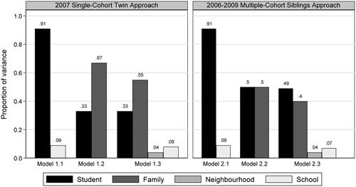
Model 1.1, the simple students-within-schools model, shows that 9% of the variation in student achievement (having adjusted for twin status) lies between schools. This figure is low compared to what we might expect in many other European countries, but is typical for Nordic countries (OECD, 2014).

Model 1.2, the simple students-within-families model, shows that 67% of the variation in twin student achievement lies between families. Thus, differences in achievement between twin families far outweigh differences in achievement between schools.

Model 1.3, which simultaneously accounts for schools, families, and neighborhoods, shows that just 8% of the variation in student achievement lies between schools and 4% between neighborhoods. In contrast, 55% of the variation lies between families, with the remaining 33% between the students themselves. Thus, the substantial importance of families persists, even after accounting for school and neighborhood effects. The results imply that 62% [0.477/(0.477 + 0.289)] of the variation in student achievement which a standard school effectiveness model would otherwise be described as between students is better described as variation between families.

Model 1.4, which extends Model 1.3 by adjusting for student age and gender, shows that adding these two covariates makes little difference to the estimated school, family, and neighborhood variance components, but slightly reduces the estimate of the student variance component. This is what we would expect at the school and neighborhood levels, where there is little variation in average age and proportion of female students across clusters. The results for student age show that being born in the first month of the academic year is associated with achievement 0.132 SD [0.012 × 11] higher than being born in the last month of the academic year. The results for student gender show female students score 0.369 SD higher than male students. This gender gap is consistent with the large gender gap reported for PISA (Programme for International Student Assessment) scores for Sweden (OECD, 2014).

Multiple-Cohort Siblings Approach Models Fitted to the Sweden 2006–2009 Data

Table 3 presents results for the “multiple-cohort siblings” approach models 2.1, 2.2, 2.3, and 2.4 (see Section “Multiple-Cohort Siblings Approach Models”) fitted to the 2006–2009 cohorts of Swedish students. We shall contrast these to the Table 2 results of “twin-family approach” models 1.1, 1.2, 1.3, and 1.4, which were fitted to the 2007 cohort of Swedish students.

Table 3. Multiple-cohort siblings approach models fitted to the Sweden 2006–2009 data.

	Model 2.1		Model 2.2		Model 2.3		Model 2.4
Parameter	Est.	SE	Est.	SE	Est.	SE	Est.	SE
Regression coefficients
Intercept	−0.010	(0.009)	0.006	(0.003)	−0.002	(0.008)	−0.198***	(0.003)
Cohort: 2006 (ref. category)
Cohort: 2007	0.011*	(0.004)	0.008	(0.004)	0.005	(0.004)	0.011**	(0.004)
Cohort: 2008	0.047***	(0.004)	0.033***	(0.004)	0.024***	(0.004)	0.040***	(0.004)
Cohort: 2009	0.057***	(0.005)	0.040***	(0.004)	0.028***	(0.004)	0.049***	(0.004)
Age within year (months)							0.012***	(<0.001)
Female							0.372***	(0.003)
Immigrant: Swedish (ref. category)
Immigrant: second generation							−0.061***	(0.012)
Immigrant: first generation							−0.066***	(0.012)
Family size: 1 child (ref. category)
Family size: 2 child							0.172***	(0.009)
Family size: 3 child							0.131***	(0.009)
Family size: 4 child							−0.013	(0.012)
Family size: 5 child							−0.146***	(0.015)
						−0.281***	(0.019)
Birth order: 1st born (ref. category)
Birth order: 2nd born							−0.136***	(0.003)
Birth order: 3rd born							−0.156***	(0.005)
Birth order: 4th born							−0.130***	(0.003)
Birth order: 5th born							−0.118***	(0.015)
Birth order: 6th (or more) born							−0.068**	(0.023)
Birth spacing: none (ref. category)
Birth spacing: close (1–24 months)							−0.013**	(0.005)
Birth spacing: wide (>24 months)							−0.029***	(0.005)
Mixed sibling sex composition							−0.017***	(0.004)
Variance components
School	0.087***	(0.004)			0.064***	(0.003)	0.058***	(0.003)
Neighborhood					0.040***	(0.001)	0.034***	(0.001)
Family			0.485***	(0.003)	0.380***	(0.003)	0.370***	(0.003)
Student	0.880***	(0.002)	0.474***	(0.003)	0.473***	(0.003)	0.432***	(0.003)
Total	0.967		0.959		0.957		0.894
Variance partition coefficients (VPCs)
Secondary school	9%				7%		6%
Neighborhood					4%	4%
Families		50%		40%		41%
Student	91%		50%		49%		48%
Model summary
Number of schools	1,298				1298		1298
Number of neighborhoods					5998		5998
Number of families with >1 sibling in model			53,754		53,754		53,754
Number of students	357,459		357,459		357,459		357,459
Deviance information criterion	969,813		909,487		892,977		865,088

Note. All models are fitted by MCMC. The estimates and standard errors are the means and SDs of the parameter chains.

Birth spacing is categorized using the time between the first and last birth within the family.

Sibling sex composition is estimated for mixed-gender siblings versus a reference category of single-sex families.

Estimation of the family effects is primarily driven by families with more than one sibling in the analysis sample. In this table, we report the number of families with more than one sibling in the analysis sample (53,754). Of these, there are 52,030 families with two siblings in the analysis sample (of these, 22,030 are from 2 child families, 18,419 from 3 child families, 7,464 from 4 child families, 2,473 from 5 child families, and 1,644 from 6+ child families), 1,723 families with three siblings in the analysis (of these 782 are from 3 child families, 470 from 4 child families, 238 from 5 child families, and 233 from 6+ child families), and just one family with four siblings in the analysis sample (also a four child family). There are many more family units (248,226) where only one of the siblings is represented in the analysis sample (of these, 22,531 are from 1 child families, 113,816 from 2 child families, 75,287 from 3 child families, 24,819 from 4 child families, 7,601 from 5 child families, and 4,172 from 6+ child families).

*p < 0.05, **p < 0.01, and ***p < 0.001.

As we would expect, model 2.1, the students-within-schools model, fitted to all four cohorts of students, shows the relative importance of schools to be effectively the same (VPC = 9%) as in model 1.1, which was fitted to only the 2007 cohort. Model 2.1 shows a trend of monotonically increasing mean achievement across the four cohorts, though we cannot say to what extent this might be a genuine increase in achievement or some other explanation such as increased teaching to the test.

In contrast, model 2.2, the students-within-families model, shows very different results to model 1.2. In model 2.2, the family variance component accounts for 50% of the variation in student achievement compared to 67% in model 1.2. This substantial 17 percentage point drop results from the different ways families are defined across the two models. In model 1.2 (and 1.3 and 1.4), families refer to twin-pair families. In model 2.2 (and 2.3 and 2.4), families refer to full siblings and maternal half-siblings as well as twin-pairs. The results suggest that twin families are relatively more different from one another and their children relatively more alike vis-à-vis families in general. This is consistent with identical twins (who make up half of twin families) sharing 100% of their genes and therefore appearing more similar to one another than siblings from the average family who typically share only 50% of their genes. Thus, how families are defined and operationalized in school effectiveness models clearly matters.

Model 2.3, which includes school, families, and neighborhood effects, again reveals that families appear less important when we use our broader definition of families (VPC = 40%) than they did in model 1.3, where families were restricted to twin pairs (VPC = 55%). Thus, now only 45% [0.380/(0.380 + 0.473)] of the variation in student achievement, which would typically be assigned directly to the students in a simple school effectiveness model, is better described as between-family variation. This contrasts our earlier reported value of 62% for model 1.3.

Figure 1 compares the estimated variance partition coefficients between the previous single-cohort twins approach models fitted to the Sweden 2007 data (Table 2, models 1.1–1.3) and the current multiple-cohort siblings approach models fitted to the Sweden 2006–2009 data (Table 3, models 2.1–2.3). The figure clearly shows how the proportion of variance described as laying between families is much larger when using the twin definition of families compared with including fuller sibship types (model 1.2 vs. model 2.2). It follows that when families are included in the school effectiveness model (model 1.3 vs. model 2.3), then a smaller proportion of the between-student variation is described as laying between families when a more realistic definition of family is used.

Figure 1. Variance partition coefficients for the three series of student achievement models using the (1) Sweden 2007 data and the twin definition of families (Table 2, models 1.1, 1.2 and 1.3); and (2) Sweden 2006–2009 data and the fuller definition of families (Table 3, models 2.1, 2.2 and 2.3).

Model 2.4 extends model 2.3 by adding not only student age and gender as in model 1.4 but also family immigration status and the four family structure characteristics: family size, birth order, birth spacing, and sibling sex composition. The interpretation of these family characteristics as specific manifestations of the family is distinct from the interpretation of the broader conceptualization of families represented by the family random effects described above.

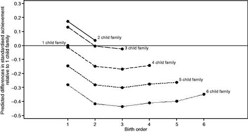
The family characteristics are interrelated, so we must interpret individual estimates with this in mind. We see that two and three child families are predicted higher achievement relative to the reference category of a one-child family (0.172 SD, 0.131 SD), this positive effect diminishes with each additional child so that families with five or six and above children have strongly negative point estimates (−0.146 SD, −0.281 SD). Alongside this, we see that relative to the reference group of firstborns, higher birth orders are all associated with lower achievement. The birth order coefficients should also be interpreted relative to the cohort effects; later-born siblings will benefit from the increasing achievement for each academic cohort, though these effects are small relative to the birth order effects and only slightly mitigate the negative effects of birth order. Where those births within a family are closely spaced, we see some evidence for a small negative effect on achievement (−0.013 SD) relative to the reference group of zero spacing (singleton, twin, and triplet only families); this penalty is larger for families with wider (>24 months) birth spacing (−0.029 SD). Finally, where families have a mixed sibling sex composition, we see a reduction in achievement (−0.017 SD) relative to single-sex families.

To aid interpretation of the combined effects of the two most substantively important family variables—family size and birth order—we present Figure 2 showing the change in predicted achievement for each combination of values observed in the data relative to a one-child family. The figure shows that family size is the dominant family structure variable associated with achievement, but that within families, there is a substantial premium associated with being the firstborn. Note that there is no interaction between these two variables in our model, so the effects of birth order are common across different family sizes. Also, in this graph, we hold all other variables constant. We note that this means that cohort and birth spacing are constrained to remain constant when we would not expect that assumption to hold as we vary family size. Including these variables would make the figure too complex to be interpretable; instead, the reader should be aware that increased spacing with increased family size would reduce predicted achievement slightly (i.e., subtract 0.013 for close spacing or 0.029 for wider spacing); the increased likelihood of mixed-sex sibship with increasing family size could subtract up to a further 0.017 from predictions; and the effect of being in later cohorts with increasing birth order effect would increase achievement slightly (i.e., add 0.011, 0.040, or 0.049 for each subsequent cohort).

Figure 2. Predicted differences in achievement (SD units) relative to a one-child family by birth order for each family size using the Sweden 2006–2009 data and the fuller definition of families (Table 3, model 2.4).

Discussion

This paper uses linked Swedish administrative data to answer two related questions: To what extent do families differ in their average educational achievements (between family variance), and to what extent do siblings differ in their individual achievements (within family variance). In doing so, we extend the important methodological and substantive contributions to this area made by Rasbash et al. (2010). In addition to describing the general importance of families when modeling achievement, we also describe how four specific family characteristics that vary within families (birth order) and between families (family size, birth spacing, sibling sex ratio) are associated with achievement. We conclude by discussing how these two findings should be interpreted alongside one another, some of the limitations of the approaches described, and finally, the implications of this study for evaluation research.

To What Extent Do Families Differ in Their Average Achievements?

The primary finding of this study is that 45% of the variation in student achievement typically described as laying between students in a standard school effectiveness model would be better described as variation laying between families. This is substantially smaller than the 62% found using the twins family approach of Rasbash et al. (which typically accounts for only 1% of all families). This reduction likely reflects the stronger genetic relatedness of identical twins (who form 50% of twin families) versus fraternal siblings (who form the vast majority of siblings in our study and populations more generally) and because both identical and fraternal twins likely share more similar environmental experiences within their families, schools, and neighborhoods than fraternal siblings.

In our models, the family effect captures shared genetic as well as shared environmental factors, while the child effect represents unshared genetic as well as unshared environmental factors. Although we did not follow the behavioral genetics approach of additionally estimating a genetic component of variation (Plomin et al., 2013), such extensions are possible with multilevel models (Guo & Wang, 2002; Rabe-Hesketh et al., 2008).

To aid the comparison of our primary finding with earlier studies, we follow Mazumder (2008) and others in calculating correlations in student achievement between students within the same school, family, or neighborhood (Table 4). Specifically, we use our model estimates to calculate intraclass correlation coefficients (ICCs) between pairs of students who share, or do not share, common families, schools, and neighborhoods. The correlation between two students from different families, who attend different schools, and live in different neighborhoods is assumed zero. We present both unconditional and conditional ICCs (based on models 2.3 and 2.4) where the latter are the correlations in student achievement after adjusting for family covariates and so measure the similarity in achievement which is not accounted for by these covariates. These ICCs are consistent with sibling correlations from earlier studies for years of schooling (Björklund & Jäntti, 2012) and earlier grades (Böhlmark & Holmlund, 2011; Holmlund et al., 2014; Skolverket, 2018), showing that students educated in the same schools or raised in the same neighborhoods show only moderately correlated achievement (0.042–0.109), while students from the same families (i.e., siblings) are very highly correlated (0.397–0.506). Collectively, these estimated ICCs can be used to inform power calculations for cluster-randomized control trials of family-level interventions.

Table 4. Unconditional (Model 2.3) and conditional (Model 2.4) intraclass correlation coefficients for student achievement among siblings, neighbors, and schools.

Family	School	Neighborhood	Unconditional intraclass correlations (Model 2.3)	Conditional intraclass correlations (Model 2.4)
Different family	Different school	Different neighborhood	0.000	0.000
Different family	Different school	Same neighborhood	0.042	0.038
Different family	Same school	Different neighborhood	0.067	0.065
Different family	Same school	Same neighborhood	0.109	0.103
Same family	Different school	Different neighborhood	0.397	0.414
Same family	Different school	Same neighborhood	0.439	0.452
Same family	Same school	Different neighborhood	0.464	0.479
Same family	Same school	Same neighborhood	0.506	0.517

Note. The correlation between children from different families, different neighborhoods, and different schools is zero by assumption.

Our findings, based on data from Sweden for cohorts completing school from 2006 to 2009, have relevance to other countries. Importantly we see that when comparable model specifications are used, the proportion of between child variation which is better described as between-family variation remains in line with estimates from the earlier Rasbash et al. (2010) study using English data despite differences in the country context, with different school systems and different proportions of between-school variation.

To What Extent Are Family Characteristics Associated With Achievement?

For our primary finding of the importance of families described above, we used a broad conceptualization of families, capturing differences in mean levels of achievement between families. In contrast, in this section, we interpret the associations of four specific family structure characteristics with student achievement. Of the family characteristics explored, family size and birth order are most important, they are also interdependent, and their effects also need to be separated from academic cohort effects as well as the factors which influence family planning decisions. All else equal, two-child families are predicted to have the highest achievement, but within any given family, the results predict decreasing achievement as individuals move down the birth order. In other words, there is a substantial premium attached to being the firstborn within a family. Thus, except for the reference group of one-child families, we see that both increasing family size and increasing birth order is associated with lower achievement. These results are consistent with the literature (Iacovou, 2008; Kuo & Hauser, 1997) and are in line with resource dilution theories (Blake, 1981), and if we accept that increasing family size is a marker of economic hardship, family stress theories too (Conger et al., 2000).

Interpreting the Broad Conceptualizations of the Family Alongside Specific Characteristics of the Family

Throughout this study, we distinguish between the broad conceptualization of the family (between—and within—family variances) and the specific conception of the family using a limited number of specific family structure characteristics (family size, birth order, birth spacing, and sibling sex ratio). There is a danger of conflating the interpretation of the first (the extent to which families differ in mean achievement) with the second (why families differ in mean achievement). We show that families are an important source of variation in achievement, we also show that several family characteristics are individually important; however, our research should not be used to argue that changes to family structure would reduce inequalities in achievement. Importantly, adding the specific family characteristics described above leads to only minor reductions in the estimated between-family (0.380–0.370 SD) and within-family (0.473–0.432 SD) variance components. This means that despite the statistical and practical significance of the family variables in our model, there are many other important family characteristics (currently unobserved) that would better help explain these family differences and which might then help identify potential family-level interventions to raise student achievement

We can also use our estimated family-level ICCs to facilitate comparisons with the applied literature on the effects of conditioning on specific measures on sibling correlations. Our results show that controlling for family structure reduces the sibling correlation of between 2% and 4% depending on the commonality across other groupings. This is lower than those seen in other studies that control for family structure, albeit for different outcomes. Bredtmann and Smith (2018), modeling the outcome years of education, find that controlling for family structure (number of siblings, mother age, live with both parents) accounts for 7% of the sibling correlation (12% for completing upper secondary education and 3% for completing tertiary education). Björklund et al. (2010) model the long-run income of siblings and are also able to control for family structure (mother’s age, number of siblings, head of households marital status, family type), which leads to a reduction in sibling correlation of 5% (0.219 vs. 0.208) for men and 11% (0.227 vs. 0.202) for females.

Limitations

An important limitation of all observational studies modeling family structure characteristics on student achievement and individual outcomes more generally is that these characteristics are endogenous. For example, the number of children parents choose to have will correlate with unobserved family characteristics (confounders or omitted variables) that might influence student achievement, such as socioeconomic status, parental attitudes to education, and behaviors that support education. For example, when we interpret our family size estimate, we may be, on average, comparing more affluent smaller families with less affluent larger families. In this case, the negative effect of family size partly reflects differences in socioeconomic status by family size. If we were able to control for affluence and other unobserved confounders, the effect of family size would reduce. Studies that use instrumental variables for family size, such as twin births as an exogenous shock to family size (Black et al., 2005) or parents’ preference for male offspring, can potentially get closer to estimating the causal effects of these influences on student achievement. While recognizing this limitation, our results are still of value as descriptive modeling of the associations, providing a starting point for other studies to attempt to estimate causal effects with richer data and, in turn, more sophisticated methods.

Similarly, the data we analyze does not provide any measure of student prior achievement and only a limited set of other background characteristics. As a result, the estimated school effects in our model will reflect not just variation in the effectiveness of these institutions, but also school differences in the prior achievement, demographic, and socioeconomic status of students when they entered their schools. Thus, our results likely overstate the true importance of schools as a source of influence on student achievement, and our models are therefore not value-added models of school effectiveness (Goldstein, 1997; Leckie & Goldstein, 2009, 2019). However, as discussed in Section “Model Assumptions,” where prior achievement is available, it will account for some of the family effect we wish to estimate, so it should be used with caution as one may understate the importance of families.

An implicit assumption of our multilevel models is that the estimates for student characteristics are the same within and between clusters. It is always prudent to estimate alternative model specifications to explore how well this assumption holds. In a fixed-effects specification, the clusters are entered as dummy variables, so the predictor effects are interpreted as purely within-cluster effects. Alternatively, in a between-effects specification, we model the relationships between the cluster averages of the data, and so the predictors are only interpreted as purely between cluster effects. Comparing a specification with full controls and a family level cluster (results not shown), we see the estimates for gender and month of birth are almost identical across fixed-effects and between-effects specifications. In terms of the other covariates, they maintain the same approximate magnitude, and so we draw qualitatively the same conclusions. We note that one would expect differences for variables such as birth order as we only have a subset of the families in the analysis sample.

The statistical methods for including family covariates and between-family variation in our models could be extended in several directions. Firstly, extending the model specification of the existing family structural characteristics (e.g., interactions between birth order and family size, more flexible modeling of birth spacing, and alternative sibling sex ratio measures). Secondly, to include richer measures of family characteristics (e.g., mother’s age, parental education, family income) and exploit upcoming data linkage for Swedish administrative data to include measures of prior achievement. Thirdly, improving the aggregated student achievement measure, either by aggregating across common core subjects or including a principal components model to account for differences in subject choices. Fourthly, one could relax the assumption of constant variance within clusters, or even modeling within (and between) family variation (Leckie et al., 2014).

While we have shown that multilevel models naturally extend to account for multiple sources of clustering simultaneously, it does not follow that researchers should automatically adjust for every level of clustering they see in their data. For example, while it is essential for statistical analyses of family-level interventions on student outcomes to account for family-level clustering to recover the correct standard errors and avoid the risk of making Type I errors of inference, there is far less need to do so in school- or student-level interventions where it is schools or students rather than families that are randomly assigned to the intervention. Abadie et al. (2017) provide detailed guidance on when and when not to account for clustering, especially in relation to clustered sample designs vs. clustered experimental designs and level of treatment assignment in interventions.

Implications for School Effectiveness Studies and Family-Level Interventions

The key implication of this study is that families should be included more often in school effectiveness models; however, the availability of suitable data is critical. Such data are routinely collected in Sweden, Denmark, Finland, and Norway, both for academic research and evaluating public policy. Thus, in these contexts, our approach could easily be adopted by others. Furthermore, rich administrative educational data are increasingly becoming available for research and evaluation in several other countries (Wales, Scotland, Australia, Canada, USA). Confirmatory analysis for these countries would help refine the message of the importance of families. Finally, linking these administrative school records and family IDs to richer school or family-based surveys could provide the measures required to progress this from descriptive analysis to a more causal framework.

A second key implication of this study is that family clusters should be considered more often as the level of intervention in educational effectiveness programs and the family-level ICCs that we report can help inform the power calculations necessary for their randomized control trials. However, the implementation of educational interventions directed at the family poses several challenges, not least competing with efficiencies from a historical academic infrastructure of school-based educational interventions. Access to households to conduct interventions are more limited than for those targeted at schools and teachers, the extant family-based instrument for interventions of cash transfers are fairly blunt tools, though perhaps the emergence of more digital innovations and the increase in contact between families and schools during the COVID-19 pandemic may provide new opportunities (Weixler et al., 2020). The additional challenges in working with families will also affect the extent to which the fidelity of these family-based interventions can be observed (Vaden-Kiernan et al., 2018). Even within school-based interventions, there is a persistence in the “grammar of schooling,” interventions that deviate from these standard approaches to teaching, learning, and knowledge tend to be challenging to scale up due to entrenched beliefs, so family-based interventions will require more than just robust evidence (Sarama et al., 2008).

Family-focused interventions to improve educational outcomes include those emphasizing the importance of role-modeling and extra-familial adults, such as the Contract Family Program in Sweden (Brännström et al., 2013), and similar mentoring and relief programs in the United States (Rhodes & DuBois, 2008). Such state-sponsored programs are rolled out with little thought for rigorous evaluation of the intervention. One large UK family-focused intervention, “Sure Start,” was supported by extensive data collection. Though the intervention was primarily clustered by regions, because of the location of centers (with most evaluations using this higher level geographic cluster), many of the key services were targeted at families. Despite family-level data being published for a subset of 2,568 families (Hall et al., 2019), there has not yet been a study that links siblings to estimate the importance of family clustering for an intervention estimated to have cost £1.8 billion per year ($2.4 billion) at its peak (Cattan et al., 2019).

Interventions that operate through improving the health of children (or parents) can evaluate the effect on child outcomes beyond health, including educational achievement, using linkage to administrative data for longer-term follow-up of a trial. Such interventions are often targeted at the family level. For example, interventions to improve parents' mental health has the potential to raise childrens' educational attainment. However, the challenge of endogeneity may compromise modeling since unobserved characteristics of the family may be associated with the propensity for mental health issues in children, with randomization by family cluster (rather than child) likely to be a costly way to achieve a sufficient sample (Hoagwood et al., 2007). Many other childhood health conditions also present a heavy burden of care or self-management on children and families. Though conditions may directly affect just one child per family, the effect on the educational achievement of the target child may be significant and have spillover effects for siblings. For example, pediatric (type 1) diabetes, one of the most common childhood chronic conditions, requires a daily regimen of blood glucose measurements and self-medication (both at home and in schools). While the occurrence of pediatric diabetes does have a genetic component (siblings are eight times more likely to be diagnosed than a random child), it is assumed to be unrelated to family characteristics that are known to affect achievement. Conversely, diabetes self-management and the resultant blood glucose levels are related to family characteristics and educational achievement, and so would be amenable to family-level interventions and would benefit from the inclusion familiy clustrs (as well as observed characteristics of the family) in modeling (Souza et al., 2021).

Additional information

Funding

This research was supported in part by grants from the ESRC [RES-576-25-0032, ES/K000950/1, ES/V017314/1, ES/R010285/1, ES/V017314/1] and MRC [MR/N015428, MC/PC/21031].

References

- Abadie, A., Athey, S., Imbens, G. W., & Wooldridge, J. (2017). When should you adjust standard errors for clustering? https://www.nber.org/papers/w24003.
- Aitkin, M., & Longford, N. (1986). Statistical modelling issues in school effectiveness studies. Journal of the Royal Statistical Society. Series A (General), 149(1), 1–43. https://doi.org/10.2307/2981882
- Benito, R., Alegre, M. Á., & González-Balletbó, I. (2014). School segregation and its effects on educational equality and efficiency in 16 OECD comprehensive school systems. Comparative Education Review, 58(1), 104–134. https://doi.org/10.1086/672011
- Berg, J., Morris, P., & Aber, L. (2013). Two-year impacts of a comprehensive family financial rewards program on children's academic outcomes: Moderation by likelihood of earning rewards. Journal of Research on Educational Effectiveness, 6(4), 295–338. https://doi.org/10.1080/19345747.2012.755592
- Björklund, A., & Jäntti, M. (2012). How important is family background for labor-economic outcomes? Labour Economics, 19 (4), 465–474. https://doi.org/10.1016/j.labeco.2012.05.016
- Björklund, A., Lindahl, L., & Lindquist, M. J. (2010). What more than parental income, education and occupation? An exploration of what Swedish siblings get from their parents. The BE Journal of Economic Analysis & Policy, 10(1), 102.
- Björklund, A., Lindahl, M., & Sund, K. (2003). Family background and school performance during a turbulent era of school reforms. Swedish Economic Policy Review, 10.2003(2), 111.
- Black, S. E., Devereux, P. J., & Salvanes, K. G. (2005). The more the merrier? The effect of family size and birth order on children's education. The Quarterly Journal of Economics, 120(2), 669–700.
- Black, S. E., Devereux, P. J., & Salvanes, K. G. (2011). Older and wiser? Birth order and IQ of young men. CESifo Economic Studies, 57(1), 103–120. https://doi.org/10.1093/cesifo/ifq022
- Blake, J. (1981). Family size and the quality of children. Demography, 18(4), 421–442. https://doi.org/10.2307/2060941
- Böhlmark, A., & Holmlund, H. (2011). 20 Years of changes in school: What happened to equality? (Translation). SNS.
- Booth, A. L., & Kee, H. J. (2009). Birth order matters: The effect of family size and birth order on educational attainment. Journal of Population Economics, 22(2), 367–397. https://doi.org/10.1007/s00148-007-0181-4
- Bound, J., Griliches, Z., & Hall, B. H. (1986). Wages, schooling, and IQ of brothers and sisters: Do the family factors differ? National Bureau of Economic Research.
- Brännström, L., Vinnerljung, B., & Hjern, A. (2013). Long-term outcomes of Sweden's Contact Family Program for children. Child Abuse & Neglect, 37(6), 404–414.
- Bredtmann, J., & Smith, N. (2018). Inequalities in educational outcomes: How important is the family? Oxford Bulletin of Economics and Statistics, 80(6), 1117–1144. https://doi.org/10.1111/obes.12258
- Browne, W. J. (2020). MCMC estimation in MLwiN v3. 03. Centre for Multilevel Modelling, University of Bristol.
- Browne, W. J., & Draper, D. (2006). A comparison of Bayesian and likelihood-based methods for fitting multilevel models. Bayesian Analysis, 1(3), 473–514. https://doi.org/10.1214/06-BA117
- Bryk, A. S., & Raudenbush, S. W. (2002). Hierarchical linear models: Applications and data analysis methods. Sage.
- Bu, F. (2014). Sibling configurations, educational aspiration and attainment. https://www.iser.essex.ac.uk/research/publications/working-papers/iser/2014-11.pdf
- Butcher, K. F., & Case, A. (1994). The effect of sibling sex composition on women's education and earnings. The Quarterly Journal of Economics, 109(3), 531–563. https://doi.org/10.2307/2118413
- Buckles, K. S., & Munnich, E. L. (2012). Birth spacing and sibling outcomes. Journal of Human Resources, 47(3), 613–642. https://doi.org/10.1353/jhr.2012.0019
- Castellano, K. E., Rabe-Hesketh, S., & Skrondal, A. (2014). Composition, context, and endogeneity in school and teacher comparisons. Journal of Educational and Behavioral Statistics, 39(5), 333–367. https://doi.org/10.3102/1076998614547576
- Cattan, S., Conti, G., Farquharson, C., & Ginja, R. (2019). The health effects of Sure Start. https://ifs.org.uk/uploads/BN332-The-health-impacts-of-sure-start-1.pdf
- Charlton, C., Rasbash, J., Browne, W. J., Healy, M., & Cameron, B. (2020). MLwiN version 3.05. Centre for Multilevel Modelling, University of Bristol.
- Conger, K. J., Rueter, M. A., & Conger, R. D. (2000). The role of economic pressure in the lives of parents and their adolescents: The Family Stress Model. In L. J. Crockett & R. K. Silbereisen (Eds.), Negotiating adolescence in times of social change (pp. 201–223). Cambridge University Press.
- Department for Education. (2019). Secondary accountability measures: Guide for maintained secondary schools, academies and free schools. https://assets.publishing.service.gov.uk/government/uploads/system/uploads/attachment_data/file/872997/Secondary_accountability_measures_guidance_February_2020_3.pdf
- Downey, D. B., & Condron, D. J. (2016). Fifty years since the Coleman Report: Rethinking the relationship between schools and inequality. Sociology of Education, 89(3), 207–220. https://doi.org/10.1177/0038040716651676
- Dundas, R., Leyland, A. H., & Macintyre, S. (2014). Early-life school, neighborhood, and family influences on adult health: a multilevel cross-classified analysis of the Aberdeen Children of the 1950s Study. American Journal of Epidemiology, 180(2), 197–207. https://doi.org/10.1093/aje/kwu110
- Eriksson, K. H., Hjalmarsson, R., Lindquist, M. J., & Sandberg, A. (2016). The importance of family background and neighborhood effects as determinants of crime. Journal of Population Economics, 29(1), 219–262. https://doi.org/10.1007/s00148-015-0566-8
- Gandhi, A. G., Slama, R., Park, S. J., Russo, P., Winner, K., Bzura, R., Jones, W., & Williamson, S. (2018). Focusing on the whole student: An evaluation of Massachusetts's Wraparound Zone Initiative. Journal of Research on Educational Effectiveness, 11(2), 240–266. https://doi.org/10.1080/19345747.2017.1413691
- Garner, C. L., & Raudenbush, S. W. (1991). Neighborhood effects on educational attainment: A multilevel analysis. Sociology of Education, 64(4), 251–262. https://doi.org/10.2307/2112706
- Goldstein, H. (1986). Multilevel mixed linear model analysis using iterative generalized least squares. Biometrika, 73(1), 43–56. https://doi.org/10.1093/biomet/73.1.43
- Goldstein, H. (1997). Methods in school effectiveness research. School Effectiveness and School Improvement, 8(4), 369–395. https://doi.org/10.1080/0924345970080401
- Goldstein, H. (2011). Multilevel statistical models (4th ed.). Wiley.
- Guo, G., & Wang, J. (2002). The mixed or multilevel model for behavior genetic analysis. Behavior Genetics, 32(1), 37–49. https://doi.org/10.1023/a:1014455812027
- Hall, J., Sammons, P., Smees, R., Sylva, K., Evangelou, M., Goff, J., Smith, T., & Smith, G. (2019). Relationships between families’ use of Sure Start Children’s Centres, changes in home learning environments, and preschool behavioural disorders. Oxford Review of Education, 45(3), 367–389. https://doi.org/10.1080/03054985.2018.1551195
- Hauser, R. M., & Featherman, D. L. (1976). Equality of schooling: Trends and prospects. Sociology of Education, 49(2), 99–120. https://doi.org/10.2307/2112516
- Hoagwood, K. E., Serene Olin, S., Kerker, B. D., Kratochwill, T. R., Crowe, M., & Saka, N. (2007). Empirically based school interventions targeted at academic and mental health functioning. Journal of Emotional and Behavioral Disorders, 15(2), 66–92. https://doi.org/10.1177/10634266070150020301
- Holmlund, H., Häggblom, J., Lindahl, E., Martinson, S., Sjögren, A., Vikman, U., & Öckert, B. (2014). Decentralisering, skolval och fristående skolor: resultat och likvärdighet i svensk skola. Institutet för arbetsmarknads-och utbildningspolitisk utvärdering (IFAU).
- Iacovou, M. (2008). Family size, birth order, and educational attainment. Marriage & Family Review, 42(3), 35–57. https://doi.org/10.1300/J002v42n03_03
- Joshi, H. (2002). Production, reproduction, and education: Women, children, and work in a British perspective. Population and Development Review, 28(3), 445–474. https://doi.org/10.1111/j.1728-4457.2002.00445.x
- Kanazawa, S. (2012). Intelligence, birth order, and family size. Personality & Social Psychology Bulletin, 38(9), 1157–1164. https://doi.org/10.1177/0146167212445911
- Kelcey, B., Spybrook, J., Dong, N., & Bai, F. (2020). Cross-level mediation in school-randomized studies of teacher development: Experimental design and power. Journal of Research on Educational Effectiveness, 13(3), 459–487. https://doi.org/10.1080/19345747.2020.1726540
- Kneale, D., & Joshi, H. (2008). Postponement and childlessness: Evidence from two. Demographic Research, 19, 1935–1968. https://doi.org/10.4054/DemRes.2008.19.58
- Koeppen-Schomerus, G., Spinath, F. M., & Plomin, R. (2003). Twins and non-twin siblings: Different estimates of shared environmental influence in early childhood. Twin Research, 6(2), 97–105.
- Kraft, M. A., & Dougherty, S. M. (2013). The effect of teacher-family communication on student engagement: Evidence from a randomized field experiment. Journal of Research on Educational Effectiveness, 6(3), 199–222. https://doi.org/10.1080/19345747.2012.743636
- Kuo, H.-H D., & Hauser, R. M. (1997). How does size of sibship matter? Family configuration and family effects on educational attainment. Social Science Research, 26(1), 69–94. https://doi.org/10.1006/ssre.1996.0586
- Leckie, G. (2009). The complexity of school and neighbourhood effects and movements of pupils on school differences in models of educational achievement. Journal of the Royal Statistical Society: Series A (Statistics in Society), 172(3), 537–554. https://doi.org/10.1111/j.1467-985X.2008.00577.x
- Leckie, G. (2013). Cross-classified multilevel models – Concepts. LEMMA VLE, Centre for Multilevel Modelling, University of Bristol, Module 12, 1-60.
- Leckie, G., & Charlton, C. (2012). runmlwin – A program to run the MLwiN multilevel modelling software from within Stata. Journal of Statistical Software, 52(11), 1–40. https://doi.org/10.18637/jss.v052.i11
- Leckie, G., French, R., Charlton, C., & Browne, W. (2014). Modeling heterogeneous variance–covariance components in two-level models. Journal of Educational and Behavioral Statistics, 39(5), 307–332. https://doi.org/10.3102/1076998614546494
- Leckie, G., & Goldstein, H. (2009). The limitations of using school league tables to inform school choice. Journal of the Royal Statistical Society: Series A (Statistics in Society), 172(4), 835–851. https://doi.org/10.1111/j.1467-985X.2009.00597.x
- Leckie, G., & Goldstein, H. (2019). The importance of adjusting for pupil background in school value‐added models: A study of Progress 8 and school accountability in England. British Educational Research Journal, 45(3), 518–537. https://doi.org/10.1002/berj.3511
- Lindahl, L. (2011). A comparison of family and neighborhood effects on grades, test scores, educational attainment and income—Evidence from Sweden. The Journal of Economic Inequality, 9(2), 207–226. https://doi.org/10.1007/s10888-010-9144-1
- Lindquist, M. J., Sol, J., Van Praag, M., & Vladasel, T. (2016). On the origins of entrepreneurship: evidence from sibling correlations. https://papers.ssrn.com/sol3/papers.cfm?abstract_id=2861023.
- Lundberg, E., & Svaleryd, H. (2017). Birth order and child health. https://www.diva-portal.org/smash/get/diva2:1179038/FULLTEXT01.pdf.
- Lunn, D., Jackson, C., Best, N., Thomas, A., & Spiegelhalter, D. (2012). The BUGS book: A practical introduction to Bayesian analysis. Routledge.
- Mazumder, B. (2008). Sibling similarities and economic inequality in the US. Journal of Population Economics, 21(3), 685–701. https://doi.org/10.1007/s00148-006-0127-2
- Nicoletti, C., & Rabe, B. (2013). Inequality in pupils' test scores: How much do family, sibling type and neighbourhood matter? Economica, 80(318), 197–218. https://doi.org/10.1111/ecca.12010
- Nye, B., Konstantopoulos, S., & Hedges, L. V. (2004). How large are teacher effects? Educational Evaluation and Policy Analysis, 26(3), 237–257. https://doi.org/10.3102/01623737026003237
- OECD. (2014). Resources, policies and practices in Sweden's schooling system: An in-depth analysis of PISA 2012 results. https://www.oecd.org/education/school/improving-schools-in-sweden-an-oecd-perspective.htm
- OECD. (2016). Family size and household composition. https://www.oecd.org/els/family/SF_1_1_Family_size_and_composition.pdf
- Page, E. B., & Grandon, G. M. (1979). Family configuration and mental ability: Two theories contrasted with US data. American Educational Research Journal, 16(3), 257–272. https://doi.org/10.3102/00028312016003257
- Pettersson-Lidbom, P., & Skogman Thoursie, P. (2009). Does child spacing affect children's outcomes? Evidence from a Swedish reform. https://www.ne.su.se/polopoly_fs/1.214873.1418655610!/menu/standard/file/spacing.pdf
- Plomin, R., DeFries, J. C., Knopik, V. S., & Neiderheiser, J. (2013). Behavioral genetics. Palgrave Macmillan.
- Powell, B., & Steelman, L. C. (1989). The liability of having brothers: Paying for college and the sex composition of the family. Sociology of Education, 62(2), 134–147. https://doi.org/10.2307/2112845
- Powell, B., & Steelman, L. C. (1993). The educational benefits of being spaced out: Sibship density and educational progress. American Sociological Review, 58(3), 367–381. https://doi.org/10.2307/2095906
- Rabe-Hesketh, S., Skrondal, A., & Gjessing, H. K. (2008). Biometrical modeling of twin and family data using standard mixed model software. Biometrics, 64(1), 280–288. https://doi.org/10.1111/j.1541-0420.2007.00803.x
- Rasbash, J., Leckie, G., Pillinger, R., & Jenkins, J. (2010). Children's educational progress: Partitioning family, school and area effects. Journal of the Royal Statistical Society: Series A (Statistics in Society), 173(3), 657–682. https://doi.org/10.1111/j.1467-985X.2010.00642.x
- Raudenbush, S. W. (1993). A crossed random effects model for unbalanced data with applications in cross-sectional and longitudinal research. Journal of Educational Statistics, 18(4), 321–349. https://doi.org/10.3102/10769986018004321
- Raudenbush, S. W., & Bryk, A. S. (2002). Hierarchical linear models: Applications and data analysis methods (Vol. 1). Sage.
- Raudenbush, S. W., & Willms, J. (1995). The estimation of school effects. Journal of Educational and Behavioral Statistics, 20(4), 307–335. https://doi.org/10.3102/10769986020004307
- Rhodes, J. E., & DuBois, D. L. (2008). Mentoring relationships and programs for youth. Current Directions in Psychological Science, 17(4), 254–258. https://doi.org/10.1111/j.1467-8721.2008.00585.x
- Rodgers, J. L., Cleveland, H. H., van den Oord, E., & Rowe, D. C. (2000). Resolving the debate over birth order, family size, and intelligence. American Psychologist, 55(6), 599–612. https://doi.org/10.1037/0003-066X.55.6.599
- Sandberg, J., & Rafail, P. (2014). Family size, cognitive outcomes, and familial interaction in stable, two-parent families: United States, 1997-2002. Demography, 51(5), 1895–1931. https://doi.org/10.1007/s13524-014-0331-8
- Sarama, J., Clements, D. H., Starkey, P., Klein, A., & Wakeley, A. (2008). Scaling up the implementation of a pre-kindergarten mathematics curriculum: Teaching for understanding with trajectories and technologies. Journal of Research on Educational Effectiveness, 1(2), 89–119. https://doi.org/10.1080/19345740801941332
- Skolverket. (2018). Analyser av familjebakgrundens betydelse för skolresultaten och skillnader mellan skolor. https://www.skolverket.se/download/18.6bfaca41169863e6a65d200/1553967875648/pdf3927.pdf.
- Snijders, T., & Bosker, R. (2012). Multilevel analysis: An introduction to basic and advanced multilevel modeling. SAGE.
- Solon, G., Page, M. E., & Duncan, G. J. (2000). Correlations between neighboring children in their subsequent educational attainment. Review of Economics and Statistics, 82(3), 383–392. https://doi.org/10.2307/2646799
- Souza, R. S., Ryan, M., Hawkes, E., Baker, C., Davies, Y., R-Screen, J., Price, J., Pryce, R., & Souza, N. A. (2021). Questionnaire-based service evaluation of the efficacy and usefulness of SEREN: A structured education programme for children and young people diagnosed with type 1 diabetes mellitus. BMJ Open Quality, 10(3), e001337. https://doi.org/10.1136/bmjoq-2021-001337
- Spiegelhalter, D. J., Best, N. G., Carlin, B. P., & Van Der Linde, A. (2002). Bayesian measures of model complexity and fit. Journal of the Royal Statistical Society: Series B (Statistical Methodology), 64(4), 583–639. https://doi.org/10.1111/1467-9868.00353
- Stallasch, S. E., Lüdtke, O., Artelt, C., & Brunner, M. (2021). Multilevel design parameters to plan cluster-randomized intervention studies on student achievement in elementary and secondary school. Journal of Research on Educational Effectiveness, 14(1), 172–135. https://doi.org/10.1080/19345747.2020.1823539
- StataCorp. (2021). Stata statistical software: Release 17. StataCorp LP.
- Teddlie, C., & Reynolds, D. (2000). The international handbook of school effectiveness research. Psychology Press.
- Vaden-Kiernan, M., Borman, G., Caverly, S., Bell, N., Sullivan, K., Ruiz de Castilla, V., Fleming, G., Rodriguez, D., Henry, C., Long, T., & Hughes Jones, D. (2018). Findings from a multiyear scale-up effectiveness trial of open court reading. Journal of Research on Educational Effectiveness, 11(1), 109–132. https://doi.org/10.1080/19345747.2017.1342886
- Weixler, L., Valant, J., Bassok, D., Doromal, J. B., & Gerry, A. (2020). Helping parents navigate the early childhood education enrollment process: Experimental evidence from New Orleans. Educational Evaluation and Policy Analysis, 42(3), 307–330. https://doi.org/10.3102/0162373720922237
- Wichman, A. L., Rodgers, J. L., & MacCallum, R. C. (2006). A multilevel approach to the relationship between birth order and intelligence. Personality and Social Psychology Bulletin, 32(1), 117–127. https://doi.org/10.1177/0146167205279581
- Willms, J. D., & Raudenbush, S. W. (1989). A longitudinal hierarchical linear model for estimating school effects and their stability. Journal of Educational Measurement, 26(3), 209–232. https://doi.org/10.1111/j.1745-3984.1989.tb00329.x
- Zajonc, R. B. (1976). Family configuration and intelligence: Variations in scholastic aptitude scores parallel trends in family size and the spacing of children. Science, 192(4236), 227–236. https://doi.org/10.1126/science.192.4236.227
- Zajonc, R. B., & Bargh, J. (1980). The confluence model: Parameter estimation for six divergent data sets on family factors and intelligence. Intelligence, 4(4), 349–361. https://doi.org/10.1016/0160-2896(80)90028-8