A Simulation Study on Latent Transition Analysis for Examining Profiles and Trajectories in Education: Recommendations for Fit Statistics

Abstract

Latent transition analysis is an informative statistical tool for depicting heterogeneity in learning as latent profiles. We present a Monte Carlo simulation study to guide researchers in selecting fit indices for identifying the correct number of profiles. We simulated data representing profiles of learners within a typical pre- post- follow up-design with continuous indicators, varying sample size (N from 50 to 1,000), attrition rate (none/10% per wave), and profile separation (entropy; from .73 to .87). Results indicate that the most commonly used fit index, the Bayesian information criterion (BIC), and the consistent Akaike information criterion (CAIC) consistently underestimate the real number of profiles. A combination of the AIC or the AIC3 with the adjusted Bayesian Information Criterion (aBIC) provides the most precise choice for selecting the number of profiles and is accurate with sample sizes of at least N = 200. The AIC3 excels starting from N = 500. Results were mostly robust toward differing numbers of time points, profiles, indicator variables, and alternative profiles. We provide an online tool for computing these fit indices and discuss implications for research.

Keywords:

• Latent transition analysis
• learning patterns
• education
• information criteria
• simulation study

Educational researchers are often interested in studying heterogeneity in learning. For whom and under what conditions does an educational intervention work? How do learners differ from each other on central learning outcomes? How do they differ concerning their learning trajectories? Reasons for heterogeneity in learning are manifold and include characteristics of learners as well as characteristics of the learning context, such as the class, teacher, school, or home (e.g., Hattie, 2009; Brühwiler and Blatchford, 2011). Usually, not all covariates that determine individual differences in learning are known. This means that there is unobserved heterogeneity, such that we do not have the information available to identify differences in learning patterns. When this is the case, it remains unstudied for whom “average” patterns of learning across a whole population are representative, leaving important aspects of heterogeneity in learning unobserved. For modeling such unobserved heterogeneity, person-centered statistical approaches are commonly used (Harring & Hodis, 2016). In these approaches, instead of correlating different variables across all learners, the learners are assigned to sub-groups based on their observed patterns on outcome variables. These sub-groups, called classes or profiles, capture individual differences in the learning process.

In the present research, we conduct a simulation study to examine the adequacy of different fit indices for the person-centered, longitudinal approach of latent transition analysis with continuous indicator variables (LTA; Hickendorff et al., 2018). In an LTA with continuous indicators, learners are grouped into latent profiles based on their patterns of means and variances across multiple variables that capture aspects of the learning process (e.g., achievement, knowledge, or motivation). In addition, capitalizing on longitudinal information, the probability that the learner's transition (i.e., switch) between different profiles over time is modeled. In educational research, these transitions would typically represent learning. A difficult aspect of the specification of these models is that the user has to decide how many latent profiles of learners should be modeled (Hickendorff et al., 2018). Usually, this decision is based on different fit statistics. In the present study, we conduct a simulation study to examine which fit statistics work best for selecting the correct number of profiles in a latent transition analysis.

Person-Centered Approaches to Studying Heterogeneity among Learners

Whereas variable-centered approaches focus on examining links between learner or context characteristics and learning outcomes, person-centered approaches aim at grouping learners according to distinct learning characteristics. Person-centered approaches have been proven useful tools to describe how learners differ at a single time point or in their learning trajectories across multiple time points (Hickendorff et al., 2018). LTA is one informative statistical tool for examining these questions that have been recently established in educational research. In this type of person-centered analysis, learners are clustered into homogenous subgroups according to their measured values on multiple variables that are meant to capture the learning process. LTA has been used, for example, to study the structure and development of children’s knowledge about density and buoyancy force (Edelsbrunner et al., 2015, 2018; Schneider & Hardy, 2013), psychology students’ understanding of human memory (Flaig et al., 2018), secondary school students’ understanding of rational numbers (Kainulainen et al., 2017), and motivational development across multiple subjects (Costache et al., 2021; Franzen et al., 2022). Cross-sectional versions of person-centered approaches have been used, for example, to identify learners at risk of developing reading disabilities (Swanson, 2012), low literacy (Mellard et al., 2016), motivational patterns across subjects (Gaspard et al., 2019), patterns of competence levels across multiple skills in science (Schwichow et al., 2020), or maladaptive learning strategies (Fryer, 2017).

Fit Indices for LTA

A central question in LTA concerns the number of profiles or clusters in the final model. For example, is a two-class model superior to a three-class model to describe literacy profiles in a sample of adolescent and young adult learners? One helpful guide in estimating the number of expected profiles or clusters in a sample is educational theory. However, theory alone is usually not sufficient for deciding on the number of expected profiles. In that case, statistical indices are required to help to decide on the number of profiles. For example, when studying profiles of conceptual knowledge, it may be theoretically sound to extract two profiles (one defined by many misconceptions, and one scientific profile; Edelsbrunner et al., 2018; Schneider & Hardy, 2013), three profiles (misconceptions, fragmented knowledge, and scientific profile), four profiles (misconceptions, fragmented knowledge, indecisive profile, and prescientific profile), or even more depending on the theoretical framework and the measurement model. Researchers need additional criteria to decide which model is best suited to characterize learners in their sample. Model fit indices, that is, statistical criteria to decide on the best fitting model regarding the number of profiles/clusters are an important tool in this regard.

Typical statistical comparisons, such as likelihood ratio tests cannot be used for determining the right number of profiles in person-centered models. The reason is that a model with one profile less can be expressed as the model with one profile more but the parameters of one profile are fixed to 0. In such cases, the difference in likelihoods of two models does not follow a known distribution that would allow computing reliable p-values (Peugh & Fan, 2013). For cross-sectional person-centered models, such as latent class and latent profile analysis, adaptations of significance tests are available to determine the best fitting solution (Hickendorff et al., 2018). For example, the bootstrap likelihood ratio test (BLRT) can be used to determine whether there is a significant increase in model fit between the more parsimonious k-1 class and the k class model (Nylund et al., 2007). For longitudinal data, as it is used in LTA, such significance tests are not available (Gudicha, Schmittmann, Tekle, et al., 2016). The reason is that the BLRT becomes computationally infeasible with large data sets and sample sizes (Tolvanen, 2007; but see Gudicha, Schmittmann, Tekle, et al., 2016 for a proposed solution). Instead, commonly employed model fit statistics for latent transition analysis are so-called information criteria, a type of relative model fit index. They are called relative because their values can only be interpreted in comparison to the values obtained from other models, for example, when comparing a two- and a three-profile LTA model. The model with lower values on the information criteria has a better fit to the data, as they incorporate statistical information of model misfit. There are several information criteria that can be used to assess relative model fit in latent transition analysis. Statistical analysis software usually provides a set of several of these indices (e.g., AIC, BIC, and sample-size adjusted BIC in Mplus). Different information criteria draw mostly on the same statistical information when evaluating a latent profile solution: The fit of the model to the data (the likelihood), model complexity (usually the number of parameters), and for some information criteria sample size. Whereas they are based largely on the same statistical information, the indices differ in the ways of combining this information. For example, the commonly used Bayesian Information Criterion (BIC) penalizes model complexity more strongly than the Akaike Information Criterion (AIC) and others (Vandekerckhove et al., 2015). In general, all relative fit indices add the penalty to the model likelihood for that depends on the number of model parameters, and sometimes sample size, to find a balance between model complexity and a fit. This raises the question of how much penalty is the right amount for LTA in educational contexts, and which fit index adds just this right amount of penalty to the likelihood. In the present study, we conduct simulations to examine the adequacy of five of these fit indices for deciding on the number of profiles in latent transition analysis. To help readers understand the commonalities and differences between different relative fit indices, we provide a conceptual overview of the indices included in this study.

Background Information on Model Fit Indices for LTA

In our study, we compare the rather well-known fit indices AIC, BIC, and aBIC (sample-size adjusted BIC), and, in addition, two further alternatives, the AIC3 and the CAIC (consistent AIC).

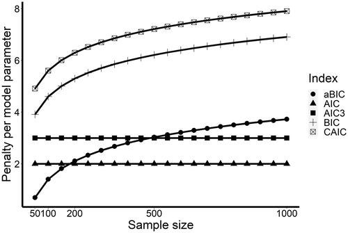
The AIC is computed as (1) $$AIC=-\text{2LL}+\text{2}p$$(1) where LL is the natural logarithm of the likelihood (the fit of the model to the data) and p is the number of model parameters, reflecting model complexity. The model parameters that have to be estimated in a latent transition analysis (for the model equation, see e.g. Edelsbrunner, 2017, p. 24; for a description of the model, see Supplementary Materials S3) are the mean values and variances of each latent profile for each of the indicator variables, the proportions of learners within each of the latent profiles (the last remaining one of which however is not estimated because it just adds up to the full proportion of 100%), and transition probabilities between all the profiles between all of the measurement points (of which as well the last one always adds up to 100%). More complex models generally lead to a better overall fit to the data, or a lower −2log likelihood. With increasing model complexity, the likelihood of overfitting increases, that is, it becomes more likely to estimate model parameters (in the present cases, profiles and transitions between these over time) that mostly catch nuisance or variance caused by sampling error (Vandekerckhove et al., 2015). The AIC counters overfitting by putting a penalty of two points on top of the −2LL for each model parameter. This penalty term was meant to select the model that has would be expected to have the lowest error in predicting future data taken from the same population as the sample data (Dziak et al., 2020). This penalty on model complexity is still relatively weak and might be too weak particularly in small samples (Dziak et al., 2020), leading the AIC to prefer rather complex models. This can be seen in Figure 1, where the penalty that different fit indices put on each model parameter is presented.

Figure 1. Penalty per model parameter that the different fit indices pose on models, depending on sample size.

Another popular fit index, the BIC, is computed as (2) $$BIC=-\text{2LL}+\text{log}\left(n\right)p$$(2)

This index puts a penalty of log(sample size) times the number of parameters on top of the −2log-likelihood. This penalty term makes the BIC stricter in terms of model complexity (see Figure 1). The reason is that this index is not meant to provide the best predictive accuracy, which might be better obtained with a weaker penalty, but it is meant to point to the true model of the data-generating process (for a more detailed description, see Aho et al., 2014). Already in small samples of up to N = 200, this index puts about 4–5 points of penalty on each parameter. Consequently, the BIC tends to favor less complex models than the AIC, for example, models with a lower number of profiles in LTA.

A third popular fit index, the sample-size adjusted BIC, is computed as (3) $$aBIC=-\text{2LL}+\text{log}\left(\left(n-\text{2}\right)/\text{24}\right)p$$(3)

The dependence on sample size here is such that in smaller models, the aBIC puts less penalty on each model parameter than the AIC, whereas for sample sizes of about N = 200 and above, it adds more penalty for each parameter than the AIC (Figure 1). Although the adaptation of the penalty term for this index has been developed for time series models, it has been found to work well, for example, in latent class models (Dziak et al., 2020).

Another alternative is the AIC3 (Fonseca, 2018), which functions similarly to the AIC but just adds three instead of two points of penalty for each model parameter: (4) $$AIC3=-\text{2LL}+\text{3}p$$(4)

Whereas the increase in the penalty of one point in comparison to the AIC is arbitrary from a theoretical view, the AIC3 has been found to work well in some studies (Dziak et al., 2020).

Finally, the consistent AIC (Vonesh & Chinchilli, 1997) puts the highest penalty on each model parameter (Figure 1), exactly one point more for each parameter than the BIC: (5) $$CAIC=-\text{2LL}+\left[\text{log}\left(n\right)+\text{1}\right]p$$(5)

The stronger penalty term in comparison to the BIC has no firm statistical basis (Dziak et al., 2020) but empirically it might work well for some models.

The differences in how these fit indices balance fit, sample size, and model complexity indicate that when comparing the fits of models that differ in the number of extracted profiles/clusters, different model fit indices may indicate different model choices. This can be seen in examples from the applied literature in which the different fit indices disagreed regarding the best solution. For example, Flaig et al. (2018) used latent transition analysis to model university students’ development of knowledge about human memory across four-time points. They estimated models with increasing numbers of profiles based on three indicator variables that captured students’ affirmative answers that were in accordance with a common misconception, a partially correct conception, and a scientifically correct concept of human memory, respectively. The authors estimated models with up to five profiles, resulting in the fit indices shown in Table 1. The AIC and adjusted BIC indicated that the five-profile model had the best fit for the data, whereas the BIC and CAIC favored the three-profile solution. The AIC3 yielded the same lowest value with three and four profiles. This raised the question of which fit index should be preferred in this data situation: Should we rely on the more stringent BIC and CAIC regarding model complexity and decide to model three profiles, or should we model five profiles based on the less stringent AIC and aBIC indices? This question is central to the present study: As different fit indices put different amounts of penalty on model complexity, researchers require guidance regarding at which sample sizes (and further factors that may affect the precision of fit indices), how much penalty is right for finding the correct number of profiles, and which fit index adds just this right amount of penalty to the respective model log-likelihood. In the study by Flaig et al. (2018), the authors decided to model four profiles, as the additional profile that appeared in the four-profile solution compared to the model with three profiles was of theoretical interest. The authors referred to the BIC as a reason not to include the fifth profile. We will come back to this example to see whether the results that we obtain from the present study support the authors’ decision, or would have suggested a different solution.

Table 1. Fit indices were obtained in the study by Flaig et al. (2018).

Number of profiles	Number of parameters	Log-likelihood	AIC	BIC	aBIC	AIC3	CAIC
1	24	−1513	3074	3144	3067	3098	3168
2	25	−1350	2750	2823	2743	2775	2848
3	41	−1278	2638	2758	2627	2679	2799
4	63	−1245	2616	2800	2599	2679	2863
5	91	−1212	2606	2872	2581	2697	2963

Note. The sample size was N = 137. Fit indices are computed based on the number of parameters and log-likelihood values reported by authors.

Situations in which different fit indices disagree are rather the rule than the exception when using latent transition analysis (e.g., Edelsbrunner et al., 2018; Flaig et al., 2018; Schneider & Hardy, 2013). Particularly in small samples (Ns < 500), under conditions of imperfect measurement (indicator variables with measurement error), study dropout, or model misspecification, fit indices may lack accuracy in determining the correct number of classes or profiles (Peugh & Fan, 2013). Researchers need to rely on guidelines regarding which model fit indices will most likely reflect the best model choice for an analysis at hand.

LTA in Educational Research: An Applied Example

For the present study, we construct another example in which we describe hypothetical learner profiles and learners’ transitions between these profiles in the course of learning. We base this example on typical design characteristics and results from previous studies that have used LTA, or related cross-sectional models, in educational research (e.g., Flaig et al., 2018; Fryer, 2017; McMullen et al., 2015; Schneider & Hardy, 2013; Straatemeier et al., 2008; Van Der Maas & Straatemeier, 2008). The online Supplementary Materials provide an extended description of the characteristics of these prior studies and how they influenced the current scenario. This example scenario serves two purposes: (1) It illustrates the questions researchers are faced with when conducting LTA, and (2) it describes the central scenario for data simulations of the current simulation study.

Let us assume that we have collected data in a longitudinal study with a group of learners at three measurement points. The three measurement points represent a pretest before an intervention, a posttest after the intervention, and a follow up-test later after the intervention. The learners answered the same knowledge test at each measurement point. Based on learners’ answers, the researchers calculated scores on each of the three continuous indicator variables at each individual measurement point. The three indicator variables represent indicators of an idealized developmental progression from preconceptions (Indicator 1) over intermediate concepts (Indicator 2) to scientifically correct concepts (Indicator 3). In this scenario, Indicator 1 represents a measure of early, scientifically incorrect knowledge. Students who are in an early stage of learning in science will show above-average scores on this indicator, for example, a misconception of rational numbers or density (see e.g., Hardy et al., 2006; McMullen et al., 2015). Indicator 2 represents a measure of intermediate knowledge. This could be an intermediate concept that is not in full accordance with scientific facts, for example, a physical concept of size and matter that does not yet fully integrate these two aspects of density (Hardy et al., 2006; McMullen et al., 2015; Schneider & Hardy, 2013). Indicator 3 represents advanced knowledge. For example, this would represent a fully scientifically correct concept of rational numbers or density.

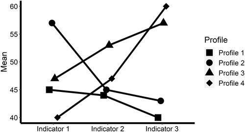
In the population, learners differ on these three indicator variables according to four underlying profiles. This is in line with prior studies, which typically identified two to five profiles (Edelsbrunner et al., 2018; Fryer, 2017; McMullen et al., 2015; Schneider & Hardy, 2013). In our example, each profile reflects a certain quality of knowledge (i.e., from naïve to expert understanding) and is characterized by its specific configuration of misconceptions (Indicator 1), prescientific concepts (Indicator 2), and scientific concepts (Indicator 3). These profiles are depicted in Figure 2; note that the indicators are centered around an arbitrary mean of 50.

Figure 2. Four latent profiles are defined by patterns of mean values across three indicator variables.

Latent Profiles

Profile 1 describes learners who show low scores on all three indicator variables, misconceptions, prescientific concepts, and scientific concepts. This represents learners who have not yet developed clear concepts, beliefs, or knowledge about a topic. Consequently, neither a high level of misconceptions nor high levels of more advanced learning progress are visible in these learners. Such profiles have been found in prior studies across various topics (Edelsbrunner et al., 2018; Flaig et al., 2018; Schneider & Hardy, 2013). Profile 2 describes students in an early stage of learning with naïve understanding, who show high levels of misconceptions (Indicator 1). Such profiles are commonly found in science education (Straatemeier et al., 2008; Van Der Maas & Straatemeier, 2008). Profile 3 describes learners who are in an intermediary stage of learning, in which they show rather high levels of prescientific concepts (Indicator 2) but also high levels of scientific concepts (Indicator 3; Edelsbrunner et al., 2015; Schneider & Hardy, 2013). Profile 4 represents a group of advanced students who have reached an (almost) expert understanding (Flaig et al., 2018).

Latent Profile Transitions

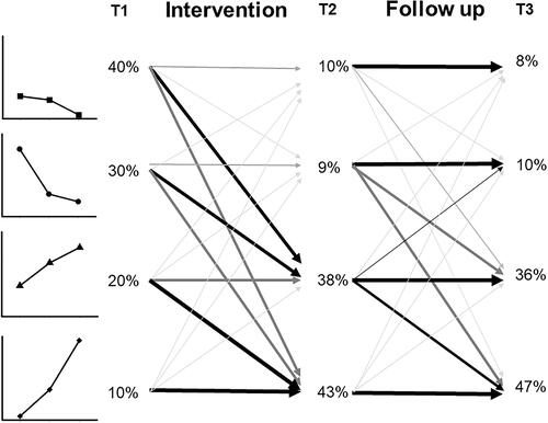
At each of the three-time points, students can belong to one of these four profiles. Educational researchers are usually interested in learners’ transitions between profiles over time. Transitions between profiles can, for example, represent learning (from pre- to posttest) or forgetting (from post-test to follow-up), depending on the nature of the profiles. Staying in the same profile can be an indicator of the absence of learning processes (from pre- to posttest), and transitioning into an initial profile may indicate a forgetting process (from post-test to follow-up). As in our example, we assumed that if there is an intervention between the first and the second measurement point, learners will most likely transition to another profile between T1 and T2. Under the assumption that the intervention is fairly effective, most learners will transition from less advanced profiles to more advanced profiles (e.g., from Profile 1 to Profile 3 or 4). The resulting transition probabilities from T1 to T2 are depicted in Figure 3. Also, as there is no further intervention, we expect that these changes will remain relatively stable between T2 and the follow-up measure at T3. Consequently, we will find high probabilities for learners to stay in the same profile between T2 and T3, with lower probabilities for transitioning back to low-quality profiles (reflecting forgetting or regressing), and also lower probabilities for advancing to higher-quality profiles (delayed learning).

Figure 3. Simulated transitions between the four profiles across the three measurement points. Note. Thicker lines indicate higher probabilities of transitioning between two profiles between two-time points. The thinnest lines indicate a 5% probability, the thickest line is 95%. Percentages at each time point indicate the resulting percentage of learners showing each profile at the respective measurement point.

Conducting the Analysis

As researchers conducting this example study, we would be unaware of the true nature of the profiles in the population (as described in the previous paragraphs and the example by Flaig et al., 2018). The question is thus, how we should decide on the number of profiles to be extracted in the analysis? From a mathematical perspective, many solutions are possible. Assuming for simplicity that learners show either low, average, or high scores on Indicators 1–3, then there are 3³ = 27 possible profile configurations at each measurement point. To analyze the underlying knowledge profiles and transition patterns throughout the three measurement points, the researcher would set up an LTA model. To allow a straightforward interpretation of the transition patterns, the researchers would constrain the indicator means and variances of each profile to be equal across the three-time points. This represents an assumption of measurement invariance, which can also be tested (Collins & Lanza, 2010). Thus, the interpretation of the profiles would not change throughout the study, that is, a misconceptions profile would show the same configuration of Indicators 1–3 at T1, T2, and T3.

To determine the number of profiles in our example, the researchers would conduct LTA and compare the fit of models with different numbers of profiles, for example, two, three, four, and five profiles. Probably, they would do some exploratory analyses with single time points first before they set up the longitudinal model to decide on the number of profiles in the final model. As there is no significance test available for LTA models, the researchers would rely on the information criteria when deciding on the number of profiles. When plotting the fit statistics of the different models, they might see an increase in fit when adding more profiles, for example, an increase in fit between the five-profile and the four-profile model. However, different fit indices may favor different model choices. For example, the BIC might indicate that the three-profile solution has the best fit for the data, whereas the aBIC might point toward the four-profile solution and the AIC toward five-profiles. For this reason, simulation studies are needed that help researchers decide which of the fit indices (or a combination thereof) works best for reliably finding the correct number of profiles.

Performance of Fit Indices: Evidence from Simulation Studies

Simulation studies can be a useful means to guide researchers’ reliance on specific fit indices in their modeling decisions. They provide information on how to fit indices perform under various modeling conditions (e.g., sample size, amount of missing data, class/profile separation, number of measurement occasions, and number of observed variables). One frequently cited publication is a Monte Carlo simulation study conducted by Nylund et al. (2007). From their analyses, the authors derived recommendations concerning the use of likelihood-based tests and information criteria in different mixture models, encompassing latent class analysis, factor mixture models, and growth mixture models. The BLRT emerged as the best performing index for model selection, followed by the BIC and adjusted BIC across the different scenarios (varying sample sizes and numbers of items) under consideration. Perhaps the consistency of these results in various modeling scenarios is a reason why the findings of the study are commonly cited in the selection process in mixture modeling (see Edelsbrunner et al., 2015; Flaig et al., 2018; Kainulainen et al. 2017; McMullen et al., 2015; Mellard et al., 2016; Schneider & Hardy, 2013; Swanson, 2012). Moreover, the findings of some other simulation studies are largely consistent with Nylund et al. (2007) in cross-sectional (Peugh & Fan, 2013; Tein et al., 2013) and longitudinal designs (Chen et al., 2017).

However, the study by Nylund et al. (2007) did not actually examine the performance of fit indices for LTA. Their study only encompassed the other mentioned kinds of mixture models. We are not aware of any simulation studies that have investigated the performance of fit statistics for identifying the correct number of classes/profiles specifically in LTA. Findings from other simulations with latent Markov models (generalizations of LTA) suggest that characteristics of the longitudinal design, such as the sample size, the number of observed variables, and the number of measurement occasions, as well as characteristics of the population model (i.e., the number of latent variables, initial proportions of the latent variables, stability of latent variable membership), are critical determinants of power when testing hypotheses in these models (Gudicha, Schmittmann, & Vermunt, 2016). Furthermore, some studies noted that the BIC should be used with caution under certain conditions, for example, because of a tendency of underfitting or generally unsatisfactory performances of all fit statistics examined (Bacci et al., 2014; Lin & Dayton, 1997; Morgan, 2015; Peugh & Fan, 2013; Tein et al., 2013). Thus, it is a matter of scientific inquiry to investigate whether findings from prior simulations conducted in cross-sectional scenarios or using other longitudinal models can be extended to latent transition analysis, particularly within the context of educational studies.

The Current Study

The current study tackles this lack of knowledge concerning the central aspect of identifying the correct number of latent classes/profiles in latent transition analysis. In this study, we simulate data from a typical scenario in educational research, specifically, the hypothetical scenario described before. In this scenario, we investigate the research question of how different fit indices perform in identifying the correct number of classes/profiles under varying conditions of sample size, participant dropout, and in the presence of more or less distinctive profiles. In addition, we will provide a robustness check to examine whether our obtained results might generalize to different scenarios and to bring up related hypotheses for future research.

Method

Simulation Scenario

We simulated data from the scenario presented in the applied example above. This scenario can be considered typical for educational research, as it resembles the average numbers of time points, indicator variables, and profiles, as well as typical profile patterns found in educational research (Compton et al., 2008; Edelsbrunner et al., 2015, 2018; Flaig et al., 2018; Fryer, 2017; Gillet et al., 2017; McMullen et al., 2015; Kainulainen et al., 2017). In our scenario, we assumed measurement invariance. In LTA, this means that the number of profiles, as well as the mean and variance parameters characterizing the profiles, remain the same across all measurement points (Collins & Lanza, 2010). We simulated four profiles and transitions of individuals between these profiles across three measurement points as presented in Figures 2 and 3.

Simulation Conditions

Whereas the described scenario was the same across all simulation runs, we varied three factors that represented our experimental simulation conditions: Sample size, entropy (profile separation), and participant dropout. An overview of the simulation conditions is presented in Table 2.

Table 2. Overview of simulated scenarios and study conditions within those scenarios.

Standard scenario	Sample sizes	Entropy	Attrition
3 indicator variables, 4 latent profiles	N = 50, 100, 200, 500, 1,000	E = .73, .82, .87	No attrition/10% attrition per wave
Robustness check scenarios	Poor conditions	Moderate conditions	Good conditions
1, 2, or 4-time points, 4 indicator variables, alternative profiles, 3 or 5 latent profiles	N = 200, E = .73, 10% attrition/wave	N = 500, E = .82, 10% attrition/wave	N = 1,000, E = .87, no attrition

As a first experimental variation, we simulated data with five different sample sizes (N = 50, 100, 200, 500, 1,000). These sample sizes covered the typical sizes found in the published literature applying latent transition analysis in education. We also included a condition with a very small sample size of only N = 50 because we sometimes encounter researchers who are interested in applying methods, such as latent transition analysis to such small datasets and who would like to know whether this might yield informative results. We caution however that with an N of only 50, the number of estimated parameters in a latent transition analysis can easily be larger than the number of observations (i.e., the sample size). In this case, many model estimators will show identification or convergence problems.

The second experimental variation in the simulations was entropy, or profile separation (Collins & Lanza, 2010). The strength of the differences between profiles is not just determined by their mean value patterns, but also by the variances of learners within the different profiles. If variances within the profiles are high, this implies that their overall distributions still overlap strongly despite the differences in mean values. If variances within the profiles are low, there is less overlap in their overall distributions, and the mean value patterns are more distinct. In the former case, when the differences in mean values are rather small compared to their variances, this results in low profile separation. The average separation or distinctiveness of profiles in an LTA model is summarized within an index called entropy. If entropy is high (close to 1), individuals belonging to different profiles can be clearly separated based on their patterns across the indicator variables. Entropy is essentially a weighted average of individuals’ posterior probabilities to belong to a certain profile given their observed patterns of values across the indicator variables (Collins & Lanza, 2010, p. 75). The formula of the entropy-index is provided in Supplementary Materials S1. If entropy is low (further away from 1, closer to 0), individuals belonging to different profiles do not so clearly show different patterns across the indicator variables, because the variances of the indicator variables overlap more strongly. We varied the variances within the four profiles, resulting in entropy values of .73 (low entropy), .82 (medium entropy), or .87 (high entropy). These values encompass most of the range of entropy estimates from prior studies applying LTA in education (see Supplementary Materials S2). We did not follow any formal rules in setting the variances and fixing entropy. Instead, to make the simulated scenario as realistic as possible, variances differed between the profiles, with those variances belonging to profiles with more extreme means fixed to be smaller (reflective, for example, of floor and ceiling effects on indicator variables) than those closer to the grand mean. We did not impose parameter constraints apart from measurement invariance over time.

The last experimental variation in the simulations was sample attrition. In educational research, the dropout of participants over time often cannot be fully avoided. In the published literature applying LTA in educational research, participant dropout varied between 0% and about 30%. We included one simulation condition in which there was no attrition and a second one with attrition. We modeled random attrition of 10% at the second and another 10% at the third measurement point, summing up to 20% of missing data after the third measurement point (this was the typical amount of missing data in prior studies, see Supplementary Materials S2).

In addition to these simulation conditions, we varied further factors in a less comprehensive manner to provide a first look into the robustness of our findings and bring up hypotheses for future research. This included the number of indicator variables in the analysis, the number of measurement points, as well as the number and nature of profiles in the population (e.g., non-linear or linear profiles, such that patterns of profile means either overlap or do not overlap across indicator variables; Hickendorff et al., 2018).

Simulation Strategy

We simulated (i.e., randomly generated applying Monte Carlo-simulation) data sets for each of the 30 (five sample sizes, three entropy levels, attrition or no attrition) conditions. Subsequently, we analyzed each dataset with latent transition analyses with varying numbers of profiles. In this way, we examined how frequently different fit indices point toward the correct solution with four profiles under each condition. We simulated and analyzed between 300 and 600 data sets for each combination of sample size, entropy, and attrition. We simulated and analyzed all data using Mplus 8.5 (Muthén & Muthén, 1998–2011) via the MplusAutomation (Hallquist & Wiley, 2018) and tidyverste (Wickham et al., 2019) packages in the R software environment (R Core Team, 2017). The number of simulated datasets was restricted by the running time of the simulations in Mplus. Although this software package is known for its fast estimation procedures for models of the kind in focus here, the estimation of a single model lasted between 1 and 30 min using multithreading on a 16-core 2.70 GHz Intel Xeon Gold 6150 Windows desktop computer with 128 RAM. All syntaxes and results-objects for R can be found under https://osf.io/w9uqy/?view_only=6c3cbdb1284346db98c7396346d06de1. Concerning the technical implementation of the simulations and analyses, we used maximum likelihood estimation with an expectation-maximization algorithm, with 400 random starts of which the most promising 100 were continued for estimation until the relative loglikelihood-change between two iterations was <10⁻⁴ and the absolute change <10⁻⁴. Further technical details are provided in the Supplementary Materials.

On each dataset, we estimated latent transition analyses with three to five latent profiles at each time point. For each estimated model, we computed the five fit indices discussed above (AIC, BIC, aBIC, AIC3, CAIC) and examined for each index whether it favored the model with three (underfitting), four (correct model choice), or five (overfitting) profiles.

Robustness Check

As a robustness check, we then selected three scenarios from our original set of factors corresponding to poor, moderate, and ideal conditions, and then verified our findings for these scenarios while changing five different aspects of the data generating process. First, we varied the number of measurement points. With only one measurement point, an LTA reduces to a latent profile analysis; latent student profiles are estimated but no transition probabilities over time, because the data are cross-sectional. To examine the robustness of our results in this cross-sectional design, we analyzed just the first measurement point of the simulated data from the standard scenario with a typical latent profile analysis model. To further examine the robustness of a design with two measurement points, we also analyzed only the first and second measurement points of the simulated data from the standard scenario by applying latent transition analysis. Finally, to examine the robustness of a study design with four measurement points, we added a fourth measurement point to the standard scenario. We then simulated transition probabilities that resembled a longitudinal study design in which there is no intervention but a more steady change between measurement points. The second characteristic that we varied for the robustness check was the number of indicator variables. We set up a scenario with a fourth indicator variable that represents another intermediate step in an educational progression, for example, in building up knowledge or skill. Details of the profiles that we set up, which resemble those for the standard scenario but with this additional intermediate indicator variable, are described in Supplementary Materials Section S2. The third characteristic that we varied for the robustness check was the number of simulated profiles. To this end, we removed one of the profiles (profile 3) but the other three profiles and their transition probabilities across the three measurement points remained the same as in the standard scenario. We also simulated a scenario with five profiles; in this scenario, the fifth profile describes learners with low values on all indicator variables. As a fourth and final characteristic, we varied the nature of the simulated profiles. To this end, we set up a scenario within which the four profiles represent motivational/affective states in which there exists less overlap than in the profiles of the standard scenario. In this way, we covered a different kind of educational research scenario in which person-centered approaches, such as LTA have also been used recently (e.g., Gillet et al., 2017) and at the same time, we covered profiles with less overlap/non-linear patterns of mean values across the indicator variables. An overview of the overall seven scenarios of the robustness check is provided in Table 1.

For the robustness check, we simulated and analyzed 300 datasets each for three benchmark conditions from among the 30 conditions of the standard scenario: Poor conditions, with a sample size of N = 200, low entropy of .73, and missing data with 10% dropout per wave; moderate conditions, with a sample size of N = 500, medium entropy of .82, and missing data with 10% dropout per wave; and good conditions, with N = 1,000, high entropy of .87, and no missing data.

Results

We report the results in three parts. First, we present the accuracy of the five fit indices under the different conditions. Accuracy is the proportion of simulated datasets for which a fit index points toward the correct model (i.e., with four profiles) under the different conditions. We summarize the accuracies of the fit indices in increasing the magnitude of sample sizes. In the second part, we examine in detail why some fit indices perform better than others. To this end, we summarize the frequencies of overfitting (selecting the model with five profiles) and underfitting (selecting the model with three profiles) for the five fit indices. In the third part, we present the results of the robustness check.

Accuracy of the Five Fit Indices across Conditions

As the simulation outcomes showed, at a sample size of N = 50, the AIC is the only fit index that could correctly identify the model with four profiles in more than 50% of cases (see Figure 4). At this extremely small sample size, all other fit indices constantly show extremely low accuracies below 15%.

Figure 4. Accuracy (proportion of correctly identified models) for the fit indices across all thirty conditions of sample size, entropy, and attrition. Note. A full horizontal line indicates 50% accuracy and dashed lines 33 and 66%.

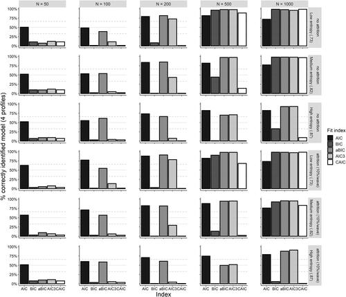
With N = 100, the accuracy of the AIC increases to about 75% across conditions, and the aBIC now is also constantly above 50%, apart from the condition with low entropy and no attrition. The accuracy of the remaining fit indices remains very low.

With N = 200, the AIC and the aBIC are constantly above 75% of correctly identified models, apart from the high entropy condition under which the performance of both appears to decrease slightly. At this sample size, also the AIC3 works better, however, its performance depends as well substantially on entropy. At the lowest level of entropy (.73), the AIC3 achieves accuracies around 75%, whereas its accuracy drops considerably below 75% in conditions of medium and high entropy. Furthermore, the AIC and the aBIC benefit from attrition in smaller samples of up to N = 200. This is visible in the higher accuracy of these two fit indices in the lower three rows compared to the upper three rows of Figure 4 at sample sizes N = 50 to N = 200. At larger sample sizes, however, the most strict model parameters BIC, AIC3, and CAIC appear to suffer moderately from attrition.

At N = 500, the AIC, aBIC, and AIC3 all demonstrate rather high accuracies. With low and moderate entropy, the aBIC and the AIC3 outperform the AIC, whereas with high entropy, the AIC outperforms the two other indices. At this sample size, the BIC and the CAIC finally show better accuracies. However, both seem to suffer from higher entropy levels. The CAIC only performs well under low entropy, and the BIC under low to medium entropy. In addition, both the BIC and the CAIC perform worse under attrition than without attrition.

At the largest sample size, with N = 1,000, all fit indices generally perform well. Only under high entropy, particularly in combination with attrition, the BIC and the CAIC lack accuracy, similarly to the patterns that they showed for N = 500.

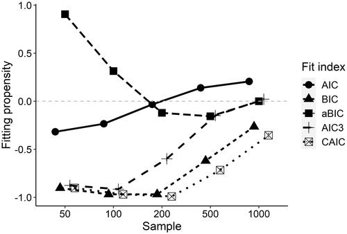
Since sample size appeared to be the decisive factor in determining the propensity of the different fit indices to find the right model, in Figure 5 it is shown how the indices behave across different sample sizes, averaged across the other factors. Marginalizing across entropy and missingness conditions, we indicated for each fit index applied to each simulated data set whether the index indicated the correct model with four profiles (indicated by a 0), underfitted (indicated by a −1), or overfitted (indicated by a 1). Averaging these values for each fit index at each sample size, we can see from Figure 5 under what sample sizes the respective fit indices tend to be overly strict (resulting in an average below 0), and tend to find the right model (resulting in values just around 0), or tend to overfit (resulting in values >0). As Figure 5 indicates, the AIC tends to slightly underfit but is the most precise index up to N = 200, where the AIC and the aBIC (which overfits up to N = 200) are both perfectly on spot. At N = 500 and N = 1,000, the AIC starts to engage in overfitting, whereas in accordance with Figure 4, the AIC3 becomes very precise and yields very similar precision as the aBIC.

Figure 5. Propensity to indicate the correct model or under- and overfit for different fit indices across sample sizes. Note. 0-line indicates perfect calibration of the fit index at respective sample size, >0 propensity to overfit, <0 propensity to underfit.

Over- and Underfitting of the Five Fit Indices across Conditions

Figures S2–S6 in the Supplementary Materials represent the frequencies of the fit indices regarding underfitting, overfitting, and identification of the correct model across the various conditions in more detail.

AIC

Overall, it is visible that in accordance with Figure 5, the reason for the moderately good, yet limited performance (50–70% of correctly identified models) of the AIC under small sample sizes is underfitting (see Figure S2). This ties back to the penalty of two points that the AIC puts on each model parameter (see Figure 1 and Equation 1(1) $$AIC=-\text{2LL}+\text{2}p$$(1) ). In samples of up to N = 100, the AIC tends to underestimate the number of profiles. At sample sizes of N = 200 and N = 500, this is not the case and AIC exhibits almost optimal performance, whereas, with N = 1,000, overfitting emerges.

BIC

As shown in Figure S3, the BIC tends to underfit (bars on grey) in smaller samples (up to N = 200). We observed an interaction between sample size and entropy on the accuracy of the BIC in larger samples of N = 500 and N = 1,000. Whereas the performance of the BIC was almost perfect in samples with low entropy, underfitting reemerged in samples with medium and high entropy (N = 500). Note that the BIC puts a strong penalty of about six points on each model parameter in such large samples (Figure 1, Equation 2(2) $$BIC=-\text{2LL}+\text{log}\left(n\right)p$$(2) ). When increasing the sample size to N = 1,000, where the penalty per model parameter increases to about seven points (see Figure 1 and Equation 2(2) $$BIC=-\text{2LL}+\text{log}\left(n\right)p$$(2) ), underfitting occurred only in conditions with high entropy.

aBIC

The aBIC showed overfitting (bars in black) in very small samples (N = 50; Figure S4). In samples of N = 100, where similar to the AIC this aBIC puts about two points of penalty on each model parameter (see Figure 1 and Equation 3(3) $$aBIC=-\text{2LL}+\text{log}\left(\left(n-\text{2}\right)/\text{24}\right)p$$(3) ), its accuracy was never far above chance. Similar to the BIC, in conditions with high entropy and a sample size of N = 500, underfitting emerged, but only in two conditions.

AIC3

The pattern of the AIC3’s accuracy was similar to the BIC, showing underfitting in various conditions (Figure S5). In larger samples, the interaction between sample size and entropy was not as strong as for the BIC. Note that the AIC3 always puts less penalty on model parameters than the BIC, particularly in larger samples (Figure 1 and Equation 4(4) $$AIC3=-\text{2LL}+\text{3}p$$(4) ). In samples of N = 1,000, the performance of the AIC3 was almost perfect and very reliable across conditions (Figure S5).

CAIC

The pattern of the CAIC, which always penalizes each model parameter more strongly than the BIC (Figure 1 and Equation 5(5) $$CAIC=-\text{2LL}+\left[\text{log}\left(n\right)+\text{1}\right]p$$(5) ), was similar to the BIC and AIC3 but with stronger underfitting except for a few conditions with large samples (N = 1,000, low to medium entropy; Figure S6).

Robustness Check

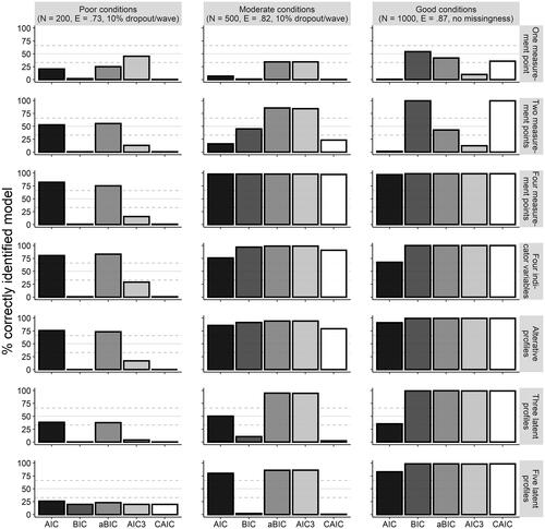
The results regarding the accuracy of the fit indices in the seven robustness check-conditions are provided in Figure 6 (the more detailed results for individual fit indices are provided in Supplementary Materials Section S4). To summarize the results from these conditions, the main conclusions from the standard scenario appear to hold. The BIC and the CAIC underestimate the actual number of profiles, particularly with just one measurement point (i.e., a latent profile analysis, with no transitions over time), with only three latent profiles, and more moderately with two measurement points or four indicator variables. The AIC works well overall but overestimates the number of profiles with only one measurement point, more moderately with two measurement points, and also moderately with three latent profiles. The aBIC works well under all scenarios. However, it tends to overfit with one measurement point. The AIC3 shows a mixed picture with both over- and underfitting with only one or two measurement points, but it works well under further scenarios apart from poor conditions. Overall, it appears that under scenarios with more linearity in the profiles (with four indicator variables and in the alternative scenario of affective/motivational profiles), as well as with four measurement points (i.e., more repeated observations of the profiles), all fit indices work better than under the standard scenario.

Figure 6. Accuracy of fit indices in the seven robustness check scenarios. Note. A full horizontal line indicates 50% accuracy and dashed lines 33 and 66%.

Discussion

Key Findings

To our knowledge, this study is the first simulation study on the performance of different fit indices for latent transition analysis applied to educational research. Overall, the results are rather clear and consistent. The AIC and aBIC showed high accuracy in smaller samples, the AIC3 in larger samples. The BIC and CAIC showed substantial underfitting, which decreased only under some conditions with the largest sample sizes and low entropy. We now discuss the more detailed results for each individual fit index and then comment on the limitations of this study and its implications for educational research.

Performance by Fit Index

Overall, the accuracy of the fit indices increased with increasing sample size. In very small samples (N = 50) the probability of identifying the correct model with four profiles was below 50% for all fit indices. In small samples (N = 100), only the performance of the AIC was more appropriate (50-75% accuracy) but far from perfect. Over- or underfitting in such small samples is more likely than identifying the correct model. In larger samples from N = 200 on, accuracy generally increases. Nevertheless, not each fit index is reliably precise in identifying the correct model in large samples of N = 500 and N = 1,000. In such large samples, our results indicate moderate overfitting for the AIC, an interaction between sample size and entropy on the performance of the BIC and AIC3, and overall insufficient accuracy of the CAIC.

The varying results between the fit indices can be traced back to how they are computed. In our descriptions of the equations of the different fit indices, we pointed out that they differ in the amount of penalty that they put on every model parameter. Our results reflect the different amounts of penalty and how they vary across sample sizes for some of the fit indices. From this view, our results can be discussed based on the question of how much penalty is adequate at what sample size. In smaller samples, the BIC, AIC3, and CAIC showed strong underfitting, the AIC moderate underfitting, and the aBIC overfitting. This can be traced back to the fact that in small samples, the BIC, AIC3, and CAIC put a higher penalty on each model parameter than the AIC and the aBIC. Apparently, the resulting penalty is too high, causing these fit indices to prefer models with too few profiles in small samples. The AIC, which puts less penalty on each model parameter, performed best in smaller samples, whereas the aBIC puts even less and too little penalty on each parameter and therefore resulted in more overfitting. In larger samples, the penalty term of the AIC3 of exactly three points for each model parameter appears to be just right for selecting the correct model. The aBIC has the same amount of penalty at N = 500, which is reflected in the comparable results for these two indices at that sample size. In contrast, starting from this sample size, the two points of penalty that the AIC puts on each model parameter are too little and this index produces overfitting.

These findings are generally in line with prior simulation studies pointing toward underfitting for the BIC in related kinds of models (Bacci et al., 2014; Lin & Dayton, 1997; Morgan, 2015; Peugh & Fan, 2013; Tein et al., 2013). The consistency of our results with the penalty terms that the different fit indices work with and with prior findings speak for their validity.

Limitations and Future Outlook

We restricted this simulation study to a design with a single group. This does not exclude our findings from informing experimental research involving multiple groups or treatments. Data from experimental studies can be analyzed with a latent transition analysis assuming a single group of students by estimating LTA models first and then relating the model parameters to a group indicator variable, for example, via the three-step approach (Nylund-Gibson et al., 2014). The effects of intervention could then, for instance, be visible in varying transition probabilities across groups, or in profiles that are reached only by individuals receiving a specific intervention (Grimm et al., 2021).

We did not assume a hierarchical data structure, for example, with students nested in classrooms or in schools. Simulation studies have shown that neglecting hierarchical data structure in similar models can lead to biased results. This problem occurs only under specific circumstances (Chen et al., 2017). Future studies should evaluate to what extent our findings generalize to such contexts.

Future research should consider our result that the fit indices with higher penalty terms BIC, AIC3, and CAIC decreased in performance under higher entropy values. Apparently, their high penalty terms come into play when the variances within profiles overlap less strongly (i.e., entropy is higher). These indices then showed underfitting. One reason for this might be that the additional variance parameters of each added profile in the model contribute less to a good model fit. There is less variance to explain around each profile’s estimated mean value. The indices, therefore, punish those parameters too much. This and further explanations for overfitting under high entropy should be evaluated in future research.

In our simulations, we considered a specific scenario, informed by published studies applying latent transition analysis in educational research (Edelsbrunner et al., 2015, 2018; Flaig et al., 2018; Kainulainen et al., 2017; McMullen et al., 2015; Schneider & Hardy, 2013). For example, we simulated data stemming from three continuous indicator variables at pre-, post-, and follow-up, and a rather specific pattern of four profiles that exhibit strong non-linear overlap in their mean values across the indicator variables, heterogeneous variances, and measurement invariance over time. It is not yet known whether our results can be fully generalized to contexts differing in these aspects. Still, this scenario is much closer to typical educational conditions than commonly cited in prior simulation studies. Such prior studies have even considered other types of models than latent transition analysis (e.g., latent class analysis and growth mixture modeling, Nylund et al., 2007), or scenarios that are further away from typical educational research regarding sample size and measurement design (e.g., intensive longitudinal studies with many more data points; Bacci et al., 2014; Gudicha, Schmittmann, & Vermunt, 2016). Thus, overall, our study appears to be the simulation study currently most closely adapted to realistic educational contexts.

We have taken a step toward generalizability by providing a few alternative conditions in our robustness check. These results are generally in line with our main findings, although they also indicate some deviations that might be further explored in future research. For example, in a scenario with more linear/less overlapping profiles, as they are commonly found in research on motivation (e.g., Costache et al., 2021) and with four indicator variables, the fit indices showed generally better performance. A deviation from our main findings was that under good conditions (e.g., N = 1,000) and with only two measurement points, the BIC and CAIC (particularly the BIC) worked better than in the other conditions. Apparently, under these conditions, the higher penalty terms of these two indices work out better. From this finding, we derive the hypothesis for future research that in an LTA with only two measurement points and a sample size of at least N = 500, the BIC is the most precise index (although note that even under these conditions, its precision was just at about 50%).

Finally, apart from the number of profiles, it would be informative to conduct simulation studies that inform about the impact of sample sizes and additional conditions on the amount of bias in the estimated profile and transition parameters. Conducting such simulation studies in mixture modeling is, however, aggravated by an issue specific to this kind of model that is called label switching (Stephens, 2000). This occurs when across different simulation runs, the profiles switch their numeric labels, such that it cannot be told which profile is which in the simulated datasets. A potential solution to this issue has been proposed that might be harnessed in future research (Tueller et al., 2011).

Implications for Educational Research

Our results show that the BIC, typically believed to be a superior fit index for mixture models (as indicated, e.g., by the very large number of articles employing this index referring to Nylund et al., 2007), performs poorly in applications of latent transition analysis to typical educational contexts. The BIC almost constantly underfits, meaning that it points toward models with too few learner profiles. This has direct implications for published research and for future research. For published research applying latent transition analysis in education, this finding indicates that reliance on the BIC for model selection might have led researchers to select models with too few profiles. We suggest researchers to re-evaluate their model selection strategies and, in case original data are still available, to re-investigate their original analyses and check whether they might have been overlooked profiles that the AIC, AIC3, or the aBIC would have detected.

In the application of LTA in educational research, we suggest putting less emphasis on model selection on the BIC and more on the AIC, aBIC, and AIC3. These indices work rather well with sample sizes of 200 individuals or more. We suggest researchers to rely more strongly on these fit indices when selecting which model to further examine and report. Optimally, this would include looking into a combination of at least two indices, for example, either the AIC for up to N = 200 or the AIC3 from N = 500 together with the aBIC. The robustness checks indicated that in cases where more linear profiles with less overlapping patterns across indicator variables are plausible or empirically found, all fit indices work better. In addition, when only one or two measurement points are analyzed, the AIC tends to overfit; in such cases, we suggest researchers to rely more strongly on the aBIC because it seems to find a better balance of complexity and fit in such scenarios. To which extent these additional results hold across further conditions should be the concern of future research. To sum up our recommendations, in Table 3 we provide an overview of guidelines for selecting appropriate fit indices among based on our findings.

Table 3. Derived guidelines for fit indices for latent transition analysis.

	Moderate sample (N = 100–200)	Large sample (N = 500–1,000)
Moderate entropy (≤.82)	AIC and aBIC	aBIC and AIC3
High entropy (≥.87)	AIC and aBIC	AIC^a and AIC3

^aUnder attrition, the weight should be shifted more toward the AIC.

Coming back to the applied example by Flaig et al. (2018), we can now see how our results would suggest solving the issue of how many latent profiles to model. At a sample size of N = 137, the entropy of .83–.86 across time points, and dropout of 17%, the AIC and adjusted BIC pointed toward five profiles, the AIC3 toward three or four, and the BIC and CAIC toward five profiles. Given our guidelines visible in Table 3, we would suggest relying more on the AIC and adjusted BIC than on the regular BIC and the CAIC, and perhaps modestly on the AIC3. Our results point toward the five profile-solution for their study and our findings regarding the BIC indicate that this index should not have been used to justify ignoring the five profile-solution. The five profile solution still could have been dropped for theoretical reasons that our study cannot inform about, such as the added theoretical information value of the fifth profile, or the amount of learners that would have been accounted for this additional profile. This example demonstrates that shifting the weight away from the BIC in realistic data situations can affect researchers’ decisions.

Readers might wonder how they should obtain the different fit indices since not all of these are provided in typical software packages that estimate latent transition analyses. We have programmed a simple online tool that researchers can freely use to compute the different fit indices. The tool is available under https://peter1328.shinyapps.io/FitApp/ and readers can use this app to compute all of these fit indices with a simple click. As a final point, we stress that prior empirical findings and established theories, as well as the researcher’s expertise should be incorporated into the model selection process. The combination of the highlighted fit indices with such information will help to prevent overlooking profiles that might be theoretically or empirically relevant, while also avoiding the extraction of profiles that might be spurious or not deliver informative insights into individual differences between learners.

Open Scholarship

This article has earned the Center for Open Science badges for Open Data through Open Practices Disclosure. The data are openly accessible at https://osf.io/42tgp.

Acknowledgments

We thank Simon Grund, Oliver Lüdtke, Gabriel Nagy, Alexander Robitzsch, and Jeroen Vermunt, as well as the organizers and attendees of the First Symposium on Classification Methods in the Social and Behavioral Sciences hosted at Tilburg University, for informative discussions and helpful feedback. Furthermore, we thank Fabian Dablander for his help with technical descriptions.

Open Research Statements

Study and Analysis Plan Registration

There is no study and analysis plan registration associated with this manuscript.

Data, Code, and Materials Transparency

The data and code that support the findings of this study are openly available on the Open Science Framework: https://osf.io/42tgp.

Design and Analysis Reporting Guidelines

This manuscript was not required to disclose the use of reporting guidelines, as it was initially submitted before JREE mandating open research statements in April 2022.

Transparency Declaration

The lead author (the manuscript’s guarantor) affirms that the manuscript is an honest, accurate, and transparent account of the study being reported; that no important aspects of the study have been omitted; and that any discrepancies from the study as planned (and, if relevant, registered) have been explained.

Replication Statement

This manuscript reports an original study.

References

- Aho, K., Derryberry, D., & Peterson, T. (2014). Model selection for ecologists: The worldviews of AIC and BIC. Ecology, 95(3), 631–636. https://doi.org/10.1890/13-1452.1
- Bacci, S., Pandolfi, S., & Pennoni, F. (2014). A comparison of some criteria for states selection in the latent Markov model for longitudinal data. Advances in Data Analysis and Classification, 8(2), 125–145. https://doi.org/10.1007/s11634-013-0154-2
- Brühwiler, C., & Blatchford, P. (2011). Effects of class size and adaptive teaching competency on classroom processes and academic outcome. Learning and Instruction, 21(1), 95–108. https://doi.org/10.1016/j.learninstruc.2009.11.004
- Chen, Q., Luo, W., Palardy, G. J., Glaman, R., & McEnturff, A. (2017). The efficacy of common fit indices for enumerating classes in growth mixture models when nested data structure is ignored: A Monte Carlo study. SAGE Open, 7(1), 215824401770045. https://doi.org/10.1177/2158244017700459
- Collins, L. M., & Lanza, S. T. (2010). Latent class and latent transition analysis: With applications in the social, behavioral, and health sciences. John Wiley & Sons.
- Compton, D. L., Fuchs, D., Fuchs, L. S., Elleman, A. M., & Gilbert, J. K. (2008). Tracking children who fly below the radar: Latent transition modeling of students with late-emerging reading disability. Learning and Individual Differences, 18(3), 329–337. https://doi.org/10.1016/j.lindif.2008.04.003
- Costache, O., Edelsbrunner, P. A., Becker, E., Sticca, F., Staub, F. C., & Götz, T. (2021). Who loses motivation and who keeps it up? Investigating student and teacher Factors for student motivational development across multiple subjects PsyArXiv Preprint. Retrieved from psyarxiv.com
- Dziak, J. J., Coffman, D. L., Lanza, S. T., Li, R., & Jermiin, L. S. (2020). Sensitivity and specificity of information criteria. Briefings in Bioinformatics, 21(2), 553–565. https://doi.org/10.1093/bib/bbz016
- Edelsbrunner, P. A. (2017). Domain-general and domain-specific scientific thinking in childhood: measurement and educational interplay [Doctoral dissertation]. ETH Zurich.
- Edelsbrunner, P. A., Schalk, L., Schumacher, R., & Stern, E. (2015). Pathways of conceptual change: Investigating the influence of experimentation skills on conceptual knowledge development in early science education. In Proceedings of the 37th Annual Conference of the Cognitive Science Society (Vol. 1, pp. 620–625). https://www.research-collection.ethz.ch/handle/20.500.11850/108017
- Edelsbrunner, P. A., Schalk, L., Schumacher, R., & Stern, E. (2018). Variable control and conceptual change: A large-scale quantitative study in elementary school. Learning and Individual Differences, 66, 38–53. https://doi.org/10.1016/j.lindif.2018.02.003
- Flaig, M., Simonsmeier, B. A., Mayer, A.-K., Rosman, T., Gorges, J., & Schneider, M. (2018). Reprint of “Conceptual change and knowledge integration as learning processes in higher education: A latent transition analysis”. Learning and Individual Differences, 66, 92–104. https://doi.org/10.1016/j.lindif.2018.07.001
- Fonseca, J. R. (2018). Information criteria’s performance in finite mixture models with mixed features. Journal of Scientific Research and Reports, 21(1), 1–9. https://doi.org/10.9734/JSRR/2018/9004
- Franzen, P., Arens, A. K., Greiff, S., & Niepel, C. (2022). Student profiles of self-concept and interest in four domains: A latent transition analysis. Learning and Individual Differences, 95(4), 102139. https://doi.org/10.1016/j.lindif.2022.102139
- Fryer, L. K. (2017). (Latent) transitions to learning at university: A latent profile transition analysis of first-year Japanese students. Higher Education, 73(3), 519–537. https://doi.org/10.1007/s10734-016-0094-9
- Gaspard, H., Wille, E., Wormington, S. V., & Hulleman, C. S. (2019). How are upper secondary school students’ expectancy-value profiles associated with achievement and university STEM major? A cross-domain comparison. Contemporary Educational Psychology, 58, 149–162. https://doi.org/10.1016/j.cedpsych.2019.02.005
- Gillet, N., Morin, A. J., & Reeve, J. (2017). Stability, change, and implications of students’ motivation profiles: A latent transition analysis. Contemporary Educational Psychology, 51, 222–239. https://doi.org/10.1016/j.cedpsych.2017.08.006
- Grimm, A., Edelsbrunner, P. A., & Möller, K. (2021). Accommodating heterogeneity: The interaction of instructional scaffolding with student preconditions in the learning of hypothesis-based reasoning. Preprint. Retrieved from psyarxiv.com/sn9c3
- Gudicha, D. W., Schmittmann, V. D., Tekle, F. B., & Vermunt, J. K. (2016). Power analysis for the likelihood-ratio test in latent Markov models: Shortcutting the bootstrap p-value-based method. Multivariate Behavioral Research, 51(5), 649–660. https://doi.org/10.1080/00273171.2016.1203280
- Gudicha, D. W., Schmittmann, V. D., & Vermunt, J. K. (2016). Power computation for likelihood ratio tests for the transition parameters in latent Markov models. Structural Equation Modeling: A Multidisciplinary Journal, 23(2), 234–245. https://doi.org/10.1080/10705511.2015.1014040
- Hallquist, M. N., & Wiley, J. F. (2018). MplusAutomation: An R package for facilitating large-scale latent variable analyses in M plus. Structural Equation Modeling: A Multidisciplinary Journal, 25(4), 621–638. https://doi.org/10.1080/10705511.2017.1402334
- Hardy, I., Jonen, A., Möller, K., & Stern, E. (2006). Effects of instructional support within constructivist learning environments for elementary school students’ understanding of “floating and sinking. Journal of Educational Psychology, 98(2), 307–326. https://doi.org/10.1037/0022-0663.98.2.307
- Harring, J. R., & Hodis, F. A. (2016). Mixture modeling: Applications in educational psychology. Educational Psychologist, 51(3-4), 354–367. https://doi.org/10.1080/00461520.2016.1207176
- Hattie, J. A. C. (2009). Visible learning: A synthesis of over 800 meta-analyses relating to achievement. Routledge.
- Hickendorff, M., Edelsbrunner, P. A., McMullen, J., Schneider, M., & Trezise, K. (2018). Informative tools for characterizing individual differences in learning: Latent class, latent profile, and latent transition analysis. Learning and Individual Differences, 66, 4–15. https://doi.org/10.1016/j.lindif.2017.11.001
- Kainulainen, M., McMullen, J., & Lehtinen, E. (2017). Early developmental trajectories toward concepts of rational numbers. Cognition and Instruction, 35(1), 4–19. https://doi.org/10.1080/07370008.2016.1251287
- Lin, T. H., & Dayton, C. M. (1997). Model selection information criteria for non-nested latent class models. Journal of Educational and Behavioral Statistics, 22(3), 249–264. https://doi.org/10.3102/10769986022003249
- McMullen, J., Laakkonen, E., Hannula-Sormunen, M., & Lehtinen, E. (2015). Modeling the developmental trajectories of rational number concept(s). Learning and Instruction, 37, 14–20. https://doi.org/10.1016/j.learninstruc.2013.12.004
- Mellard, D. F., Woods, K. L., & Lee, J. H. (2016). Literacy profiles of at-risk young adults enrolled in career and technical education. Journal of Research in Reading, 39(1), 88–108. https://doi.org/10.1111/1467-9817.12034
- Morgan, G. B. (2015). Mixed mode latent class analysis: An examination of fit index performance for classification. Structural Equation Modeling: A Multidisciplinary Journal, 22(1), 76–86. https://doi.org/10.1080/10705511.2014.935751
- Muthén, L. K., & Muthén, B. O. (1998–2011). Mplus user’s guide (6th ed.). Muthén & Muthén.
- Nylund, K. L., Asparouhov, T., & Muthén, B. O. (2007). Deciding on the number of classes in latent class analysis and growth mixture modeling: A Monte Carlo simulation study. Structural Equation Modeling: A Multidisciplinary Journal, 14(4), 535–569. https://doi.org/10.1080/10705510701575396
- Nylund-Gibson, K., Grimm, R., Quirk, M., & Furlong, M. (2014). A latent transition mixture model using the three-step specification. Structural Equation Modeling: A Multidisciplinary Journal, 21(3), 439–454. https://doi.org/10.1080/10705511.2014.915375
- Peugh, J., & Fan, X. (2013). Modeling unobserved heterogeneity using latent profile analysis: A Monte Carlo simulation. Structural Equation Modeling: A Multidisciplinary Journal, 20(4), 616–639. https://doi.org/10.1080/10705511.2013.824780
- R Core Team. (2017). R: A language and environment for statistical computing. R Foundation for Statistical Computing.
- Schneider, M., & Hardy, I. (2013). Profiles of inconsistent knowledge in children’s pathways of conceptual change. Developmental Psychology, 49(9), 1639–1649. https://doi.org/10.1037/a0030976
- Schwichow, M., Osterhaus, C., & Edelsbrunner, P. A. (2020). The relationship between the control-of-variables strategy and science content knowledge in secondary school. Contemporary Educational Psychology, 63, 101923. https://doi.org/10.1016/j.cedpsych.2020.101923
- Stephens, M. (2000). Dealing with label switching in mixture models. Journal of the Royal Statistical Society: Series B (Statistical Methodology), 62(4), 795–809. https://doi.org/10.1111/1467-9868.00265
- Straatemeier, M., van der Maas, H. L., & Jansen, B. R. (2008). Children’s knowledge of the earth: A new methodological and statistical approach. Journal of Experimental Child Psychology, 100(4), 276–296. https://doi.org/10.1016/j.jecp.2008.03.004
- Swanson, H. L. (2012). Cognitive profile of adolescents with math disabilities: Are the profiles different from those with reading disabilities? Child Neuropsychology, 18(2), 125–143. https://doi.org/10.1080/09297049.2011.589377
- Tein, J.-Y., Coxe, S., & Cham, H. (2013). Statistical power to detect the correct number of classes in latent profile analysis. Structural Equation Modeling: A Multidisciplinary Journal, 20(4), 640–657. https://doi.org/10.1080/10705511.2013.824781
- Tolvanen, A. (2007). Latent growth mixture modeling: A simulation study (No. 111). University of Jyväskylä.
- Tueller, S. J., Drotar, S., & Lubke, G. H. (2011). Addressing the problem of switched class labels in latent variable mixture model simulation studies. Structural Equation Modeling: A Multidisciplinary Journal, 18(1), 110–131. https://doi.org/10.1080/10705511.2011.534695
- Van Der Maas, H. L., & Straatemeier, M. (2008). How to detect cognitive strategies: Commentary on ‘Differentiation and integration: Guiding principles for analyzing cognitive change’. Developmental Science, 11(4), 449–453. https://doi.org/10.1111/j.1467-7687.2008.00690.x
- Vandekerckhove, J., Matzke, D., & Wagenmakers, E.-J. (2015). Model comparison and the principle of parsimony. In J. R. Busemeyer, Z. Wang, J. T. Townsend, & A. Eidels (Eds.), The Oxford handbook of computational and mathematical psychology (pp. 300–319). Oxford University Press.
- Vonesh, E., & Chinchilli, V. (1997). Linear and nonlinear models for the analysis of repeated measurements. CRC Press.
- Wickham, H., Averick, M., Bryan, J., Chang, W., McGowan, L., François, R., Grolemund, G., Hayes, A., Henry, L., Hester, J., Kuhn, M., Pedersen, T., Miller, E., Bache, S., Müller, K., Ooms, J., Robinson, D., Seidel, D., Spinu, V., … Yutani, H. (2019). Welcome to the Tidyverse. Journal of Open Source Software, 4(43), 1686. https://doi.org/10.21105/joss.01686