Combined chronic dietary exposure to four nephrotoxic metals exceeds tolerable intake levels in the adult population of 10 European countries

Abstract

A mixture risk assessment (MRA) for four metals relevant to chronic kidney disease (CKD) was performed. Dietary exposure to cadmium or lead alone exceeded the respective reference values in the majority of the 10 European countries included in our study. When the dietary exposure to those metals and inorganic mercury and inorganic arsenic was combined following a classical or personalised modified reference point index (mRPI) approach, not only high exposure (95th percentile) estimates but also the mean exceeded the tolerable intake of the mixture in all countries studied. Cadmium and lead contributed most to the combined exposure, followed by inorganic arsenic and inorganic mercury. The use of conversion factors for inorganic arsenic and inorganic mercury from total arsenic and total mercury concentration data was a source of uncertainty. Other uncertainties were related to the use of different principles to derive reference points. Yet, MRA at the target organ level, as performed in our study, could be used as a way to efficiently prioritise assessment groups for higher-tier MRA. Since the combined exposure to the four metals exceeded the tolerable intake, we recommend a refined MRA based on a common, specific nephrotoxic effect and relative potency factors (RPFs) based on a similar effect size.

Keywords:

• Cadmium
• lead
• inorganic arsenic
• inorganic mercury
• nephrotoxicity
• combined exposure

Introduction

Heavy metals like lead, cadmium and inorganic mercury are well known for their adverse effects on the kidney (EFSA 2009a, 2010b, 2012c). In fact, EFSA based its risk assessment of these metals on their nephrotoxic effects (EFSA 2009a, 2010b, 2012c). For many years, the health risks of metals were assessed based on exposure to a single metal. However, humans are chronically exposed to multiple metals in their daily life as consumers or at the workplace. This exposure occurs via different sources (e.g. food, drinking water, dust or consumer products) and via different exposure routes (oral, dermal and inhalation). The combined exposure to different metals may cumulate the risk due to dose addition (Rotter et al. 2018). Therefore, it would be more pertinent to assess the risk of combined exposure (hereinafter called mixture risk assessment [MRA]) to metals on nephrotoxicity.

In the past years, concepts, methods, guidance documents and applications for MRA haven been developed (Boobis et al. 2008; Fox et al. 2017; Bopp et al. 2018; OECD 2018; EFSA 2019, 2021b). To harmonise MRA within the European Union, EFSA has published two guidance documents for MRA. In the first report, EFSA introduced a tiered approach for several aspects of MRA across EFSA’s domains (EFSA 2019). In the second EFSA report, criteria for grouping chemicals for MRA were published (EFSA 2021b). Grouping based on mechanistic information, such as a common mode of action or adverse outcome pathway (AOP), using weight of evidence approach is regarded as the gold standard. Yet, since mechanistic data are not always available to a sufficient extent, EFSA also proposed grouping based on a common adverse outcome (phenomenon) or a common target organ/system as an alternative. EFSA used these grouping principles for dietary exposures to pesticides and proposed common assessment groups derived for chronic effects on the thyroid and for those that have acute effects on the nervous system (EFSA 2020a, 2020b). Grouping at the organ level could be regarded as a prioritisation step according to the EFSA paradigm to prioritise target organs for higher tier MRA (EFSA 2021b; Te Biesebeek et al. 2021).

In this article, we explored MRA using a component-based approach for dietary exposure to metals causing nephrotoxicity. As already mentioned cadmium, lead and inorganic mercury are well-known nephrotoxic metals and were therefore selected. Since exposure to inorganic arsenic can also cause kidney damage in humans (Foa et al. 1984; Hong et al. 2004; Lin YJ et al. 2020), we included inorganic arsenic too. Adverse effects on the kidney can be divided roughly into effects on the tubuli (cadmium, inorganic mercury) and glomeruli (lead, inorganic arsenic, inorganic mercury; Table 1). Both impact on the functioning of the kidney and may result in chronic kidney disease (CKD). Therefore, these metals can be grouped at the target organ level for MRA. MRA was performed following the modified reference point index (mRPI) approach, introduced by Vejdovszky et al. (2019). This approach sums percentiles at the population level and is hereinafter referred to as the classical mRPI approach. Further refinement of the mRPI to the individual level yields a distribution of mRPIs as described by Van den Brand et al. (2022) and Sprong et al. (2023); this approach is referred to as the personalised mRPI approach. Both approaches were applied in this article. Using food consumption data from ten European countries and metal concentration data in food from 14 European countries, we assessed the risk related to the combined dietary exposure to the four metals as well as the metals and food items driving the risk.

Table 1. Metals in the assessment group, their endpoint-specific reference value (ESRV) used in the assessment and data used for the derivation of the ESRV.

Metal	Effect	Reference point	Reference type	Species	UF	Conversion to intake dose	ESRV µg/kg bw/d	Reference
Cadmium	Elevated beta-2-microglobulin levels in urine in female volunteers aged > 50 years	4.0 µg/g creatinine	BMDL05	Human	3.9^a	Relation dietary exposure and urinary cadmium levels in non-smoking Swedish women	0.36	EFSA (2009a); Amzal et al. (2009)
Lead	Prevalence of chronic kidney disease defined as a 50% reduction in the glomerular filtration rate to values below 60 mL/min/1.73 m^2 body surface in male and female adults aged > 20 years	15 µg/L blood	BMDL10	Human	3.16^b	Carlisle-Wade model for relation between dietary exposure and lead levels in blood	0.20	Carlisle and Wade (1992); EFSA (2010b)
iAs	Estimated glomerular filtration rate of <60 mL/min/1.73 m^2 body surface in male and female adults > 40 years	1.56 µg/kg per day	BMDL05	Human	3.16^c	Physiologically based pharmacokinetic model	0.49	Lin YJ et al. (2020)
iHg	Elevated biomarkers of proteins in urine in male and female workers (average age 30 years)	35 µg/g creatinine	NOAEL	Human	10^d	Steady-state equation	0.75	SCOEL (2007)

UF: uncertainty factor; ESRV: endpoint-specific toxicological reference value; BMDL: benchmark dose lower limit, NOAEL no observed adverse effect levels, iAs: inorganic arsenic; iHg: inorganic mercury

^a Chemical-specific adjustment factor as applied by EFSA (2009a).

^b Default assessment factor for intraspecies differences in toxicodynamics.

^c Default assessment factors for intraspecies differences in toxicokinetics.

^d Default assessment factors for intraspecies differences in toxicodynamics and toxicokinetics.

Materials and methods

Hazard identification and characterisation

Lead, cadmium, inorganic arsenic and inorganic mercury were identified as priority substances within the European Human Biomonitoring Initiative HBM4EU (www.hbm4eu.eu). Exposure to these metals can impact on various organs; in this study, however, we focused on the adverse effect on the kidney as a common target organ. Grouping of these metals for MRA was based on the adverse outcome pathway (AOP) proposed in the HBM4EU project (Sarigiannis 2022).

Endpoint-specific reference values

Endpoint-specific reference values (ESRVs) were obtained for each of the four metals (Table 1) and described in more detail below.

Cadmium

For cadmium, we used the tolerable weekly intake (TWI) level of 2.5 µg cadmium/kg bw derived by EFSA (2009a). This was based on a reference point with an urinary level of 4.0 µg cadmium/g creatinine for the increased prevalence of elevated beta-2-microglobulin (a biomarker for tubular effects) levels in humans, which was obtained using the lower confidence limit after benchmark dose modelling with an effect size of 5% (BMDL₀₅; EFSA 2009a). Using a one-compartment model describing the relationship between dietary cadmium exposure and urinary cadmium excretion in Swedish women (Amzal et al. 2009) and a chemical specific adjustment factor of 3.9 for inter-individual variation in urinary cadmium, EFSA derived a health-based guidance value of 0.36 µg cadmium/kg bw/d (and subsequently a TWI of 2.5 µg cadmium/kg bw). This value of 0.36 µg cadmium/kg bw/d was used in this study as the ESRV for cadmium.

Lead

EFSA did not set a health-based guidance value (such as a tolerable weekly or daily intake) for lead, in contrast to cadmium. However, the Authority did derive a BMDL₁₀ of 15 µg lead/L blood, based on effects on the prevalence of CKD, defined as a reduction in the glomerular filtration rate to values below 60 mL/min in humans (EFSA 2010b). Using the relationship between dietary lead intake and blood levels in adults (Carlisle and Wade 1992), this internal exposure level corresponds to an external dietary exposure level of 0.63 µg lead/kg bw/d. Since the elderly, the most sensitive population for CKD, were underrepresented in the epidemiological cohort, an additional uncertainty factor (UF) of 3.16 for differences in toxicodynamics was applied, resulting in an ESRV of 0.20 µg lead/kg bw/d.

Inorganic arsenic

Recently, a BMDL₀₅ of 1.557 µg/kg bw/d was derived for the adverse effects of inorganic arsenic on the estimated glomerular filtration rate (less than 60 mL/min/1.73 m²; Lin et al. 2020). Using a cohort of 601 Taiwanese subjects aged over 40 years (mean age 64 years), those authors first modelled blood total arsenic levels into an estimated daily intake of inorganic arsenic using a physiologically based pharmacokinetic model. Subsequently, benchmark dose modelling was performed to obtain the BMDL. We applied an additional UF of 3.16 for intraspecies differences in toxicokinetics because the BMDL was based on only one population group (Taiwanese subjects) and the number of subjects included was relatively small. This resulted in an ESRV of 0.49 µg inorganic arsenic/kg bw/d.

Inorganic mercury

The no observed adverse effect level (NOAEL) of 35 µg mercury/g creatinine for elevated protein marker levels (such as increased levels of beta-galactosidase activity and increased excretion of retinol-binding protein and beta-2-microglobulin levels) in urine (Buchet et al. 1980; Roels et al. 1985; SCOEL 2007) was used as reference point. As total mercury in urine predominantly reflects inorganic mercury exposure and very little methyl mercury is excreted in urine (Berglund et al. 2005), the value of 35 µg mercury/g creatinine was extrapolated to inorganic mercury. Assuming that all inorganic mercury in urine originated from dietary exposure, a daily urinary creatinine excretion C_e of 1.5 (Hays et al. 2010), an absorption factor F_a of 0.1 (the high end of the range reported for inorganic mercury (Berglund et al. 2005; JECFA 2011; EFSA 2012c), an estimated, conservative urinary excretion factor F_ue of 1 (all absorbed inorganic mercury is excreted in urine), and a mean body weight bw of 70 kg, the creatinine adjusted urinary excretion Cc of 35 µg mercury/g creatinine was transferred into a daily dietary dose, D_dietary, using the formula: (1) $$D_{\mathit{dietary}}=\mathrm{ }\frac{\mathrm{C}c\mathrm{\hspace{0.17em}*\hspace{0.17em}}{C}_e}{F_a\mathrm{\hspace{0.17em}*\hspace{0.17em}}{F}_{\mathit{u}\mathit{e}}\mathrm{\hspace{0.17em}*\hspace{0.17em}}bw}$$(1)

Because the NOAEL was based on a limited number of adult workers (n = 185), an additional UF of 10 (3.16 for intraspecies differences in toxicodynamics and 3.16 for intraspecies differences in toxicokinetics) was used, and subsequently an ESRV of 0.75 µg/kg bodyweight was obtained. Equation (1)(1) $$D_{\mathit{dietary}}=\mathrm{ }\frac{\mathrm{C}c\mathrm{\hspace{0.17em}*\hspace{0.17em}}{C}_e}{F_a\mathrm{\hspace{0.17em}*\hspace{0.17em}}{F}_{\mathit{u}\mathit{e}}\mathrm{\hspace{0.17em}*\hspace{0.17em}}bw}$$(1) can be used in case where chronic exposure to a substance (i.e. inorganic mercury) has resulted in a steady-state situation in humans (or animals). Due to a daily, chronic exposure (via the diet) and a rather long elimination half-life of inorganic mercury in humans (40 d for mercuric mercury (EFSA 2012c)) the steady-state condition is met.

Exposure assessment

Metal concentration data

Metal concentration data used in the present MRA were obtained from the EFSA data warehouse from 13 European countries: Austria, Croatia, Cyprus, Denmark, Estonia, Finland, France, Hungary, Ireland, Italy, Lithuania, the Netherlands and Sweden. Concentration data according to EFSA’s standard sample description 1 (EFSA 2010c) for cadmium, lead, mercury and arsenic over the years 2014–2018 were extracted. In addition, national cadmium concentration data between 2014 and 2016 were extracted from the EFSA data warehouse by Portugal and added to the combined metal concentration data from the other countries. The concentration data were coded according to EFSA’s harmonised food coding system FoodEx1 (EFSA 2011). If a FoodEx code was missing, but the product name was available, the corresponding FoodEx code was added manually. Data were cleaned by removing samples obtained via targeted strategy (as such, only data obtained from random and convenient sampling were included), removing duplicate or otherwise aberrant samples, removing samples with empty fields where a value for a metal concentration or the limit of detection (LOD) was expected and removing samples with invalid concentration units. Wherever, possible food concentration data were used at the most detailed FoodEx1 level (level 4). If less than 50 samples were available, the data were grouped at a lower, less detailed FoodEx1 level. For example, ‘cow milk, < 1% fat (skimmed milk)’ was then recoded into cow’s milk (level 3), liquid milk (level 2) or milk and dairy products (level 1), wherever relevant. Aggregation to a less detailed FoodEx1 level was not performed if such aggregation would result in foods with a large difference in metal composition being grouped together (e.g. inorganic arsenic in rice-based products and wheat-based products were not grouped together).

For each metal and composite food (i.e. foods consisting of more than one ingredient) combination in the dataset, the analytical value of the composite food as such was used or converted into its ingredient(s) (see Section Matching food to concentration data). The complexity of the food (e.g. the FoodEx1 code represented a broad range of foods rather than a single food), availability of recipe data and number of measurements for the composite food and its ingredients were criteria affecting the decision made. When it was decided to convert a composite food into its ingredients rather than using the concentration data of the particular composite food, the metal concentration of the composite food was removed from the dataset. Supplemental Material A provides information on the used FoodEx1 levels and mean concentrations for each compound and food combination in the dataset, as well as the number of analytical samples and the percentage of left-censored data. Some compound-specific information regarding the concentration data are provided below.

Cadmium. Samples coded as ‘cadmium and derivatives’ were removed because additional information related to the specific compound analysed was missing. After data cleaning 39,114 entries from 14 countries and for 329 food codes were obtained.

Lead. The same concentration data for lead were used as described by Sprong et al. (2023). From the EFSA data warehouse, all samples that were analysed for ‘lead’ were retrieved. Two aberrant samples (outliers defined as larger than two times the standard deviation) were removed from the FoodEx1 category ‘wine’; one with 14 mg lead/kg and the other with 21 g/kg. Of all substances, lead concentration data were abundantly available, with 39,919 entries that were obtained from 13 European countries and for 358 different FoodEx1 codes, after clean-up of the data.

Inorganic arsenic. Concentration data used for inorganic arsenic were similar to those described in the article by Sprong et al. (2023). From the EFSA data warehouse, samples containing ‘arsenic’ were retrieved. Since we focused on the exposure to inorganic arsenic, ‘organic arsenic’ samples were omitted from the data and samples coded as ‘arsenic and derivatives’ and ‘arsenic’ were recoded to ‘total arsenic’ samples, following the approach taken by EFSA (2021a). If both ‘total arsenic’ and ‘inorganic arsenic’ values were reported for the same samples, the ‘total arsenic’ data were omitted from the database. In addition, after closer examination of the original data, samphire (‘zeekraal’) samples analysed for ‘arsenic’ from the Netherlands were originally coded as ‘leafy vegetables’, and were recoded as ‘seaweeds’. From the remaining ‘total arsenic’ samples, the fraction of inorganic arsenic was translated according to the median ratios described in EFSA’s Scientific Opinion (EFSA 2021a). Similar to EFSA, total arsenic was not converted into inorganic arsenic for fish. Supplemental Material B lists the factors used for the conversion of total arsenic into inorganic arsenic. The original dataset also contained 3104 entries for drinking water (tap and bottled). High concentrations of inorganic arsenic in tap water (typically up to 7920 µg/L), especially originating from one country, were present in the data set. In addition, the dataset contained non-detects with high LOQs (up to 900 µg/kg). In the most recent EFSA opinion on inorganic arsenic, EFSA used concentration data over the years 2013–2018 and excluded non-detects with high LOQs and high concentrations (EFSA 2021a). EFSA did not provide specific information to reproduce their cleaning step. Therefore, all entries for drinking water were replaced with the mean lower and upper bound (UB) concentrations that EFSA reported in 2021. After data cleaning, 3021 entries for inorganic arsenic were obtained from 13 EU countries and for 117 different FoodEx1 codes.

Inorganic mercury. Samples coded as ‘mercury and derivatives’ were removed because additional information related to the specific compound analysed was missing. In addition, all ‘methylmercury’ and ‘organic mercury’ entries were removed as these were not relevant for this assessment. Subsequently, the ‘total mercury’ entries were translated to ‘inorganic mercury’ according to the fractions indicated by EFSA in their exposure assessment (EFSA 2012c). Inorganic mercury was considered 20% of the total mercury reported in fish samples and 50% in shell fish samples. All other samples that reported total mercury were considered 100% inorganic mercury. After cleaning the data, a total of 14,437 inorganic mercury samples were used for the exposure assessment, obtained from 14 EU countries and for 188 different FoodEx1 codes.

Food consumption data

From 10 different European countries, Austria, Croatia, Cyprus, Czech Republic, Denmark, France, Italy, the Netherlands, Portugal and Slovenia, the most recent food consumption surveys were used in this assessment. Approval to use these data was obtained from the data owners and submitted to EFSA, after which the food consumption data was retrieved from the EFSA data warehouse. The food consumption data were coded using the harmonised food coding system FoodEx1 (EFSA 2011). If the data were originally submitted to EFSA in FoodEx2, the data were recoded by EFSA into FoodEx1. Table 2 shows an overview of the consumption data used in our study.

Table 2. Description of the food consumption data of ten different European countries included in the cumulative exposure assessment for chemicals relevant for nephrotoxicity.

	Food consumption survey						Data included in study
Country	Method^a	Years^c	Name^d	Population^e (y)	N total^g	Consumption days^h	Population^i (y)	N^j
Austria (AT)	24-h dietary recall	2016	NATIONAL-2016	18–64	2250	2	18–64	2250
Croatia (HR)	24-h and 48-h dietary recall	2011–2012	NIPNOP-HAH- 2011–2012	18–64	2002	3	18–64	2002
Cyprus (CY)	24-h dietary recall	2014–2017	2014–2017–LOT2	10–76	1016	3	18–64	478
Czech Republic (CZ)	24-h dietary recall	2004–2008	SISP04	4–64	2353	2	18–64	1666
Denmark (DK)	Food record	2005–2008	DANSDA 2005–2008	4–75	2700	7	18–64	1739
France (FR)	FPQb and 24-h dietary recall	2014–2015	INCA3	General population^f	4874	3	adults	1980
Italy (IT)	Food record	2005–2006	INRAN SCAI 2005–2006	0–97	3323	3	18–64	2313
Netherlands (NL)	Food record, 24-h dietary recall	2012–2016	FCS2016_Core	1–80	4313	2	18–64	2849
Portugal (PT)	Food record, 24-h dietary recall	2015–2016	IAN-AF-2015–2016	0–84	6429	2	18–64	3434
Slovenia (SI)	24-h dietary recall	2018	SI.MENU-2018	0–75	1981	2	18–64	1047

^a Method of food consumption survey.

^b FPQ – Food propensity questionnaire.

^c Year(s) in which the food consumption survey was conducted.

^d Name of the food consumption survey.

^e The population addressed, the population included males and females.

^f Due to privacy reasons, French food consumption data contained age groups instead of individual ages.

^g The total number of individuals included in the food consumption survey.

^h The number of consumptions days included in the study.

ⁱ The age of the subpopulation group (adults) included in the assessment.

^j The number of individuals included in the assessment.

Matching food to concentration data

Food consumption data were matched with concentration data at the same level of detail, wherever possible. When insufficient data were available to do so (e.g. in case of missing concentration data), food consumption was linked to a less detailed level of FoodEx1 coding using the hierarchical FoodEx1 system. For example, consumption of turnips was linked to concentration data in root vegetables. Concentrations of metals are often available in raw agricultural products rather than processed products. Therefore, a food translation table was used to link consumed processed food to metal concentrations in its raw agricultural commodity ingredients. For this we used a food translation table, which was based on the Dutch food translation table made for pesticides (Boon et al. 2015) and updated for animal-derived foods (Sprong et al. 2023). The food translation table was based on Dutch recipes and contained conversion factors to convert foods classified according to FoodEx1 into their edible raw agricultural commodity ingredients (e.g. 167 g raw spinach is needed to produce 100 g cooked spinach).

Metals are often considered stable in food and resistant to processing (relevant EFSA opinions). Therefore, the use of processing factors was not considered relevant.

Exposure scenarios

The exposure assessment was performed by assigning the reported samples below the limit of quantification (LOQ) or LOD with a value of zero (lower bound [LB] scenario) or with the respective value of the LOQ or LOD of the sample (UB scenario) according to EFSA and WHO practices (EFSA 2010a; mICPS 2020).

Mixture risk assessment

MRA was performed according to the classical (Vejdovszky et al. 2019) and the personalised mRPI approach (van den Brand et al. 2022; Sprong et al. 2023) and using the Monte Carlo Risk Assessment tool version 9.1 (MCRA, https://mcra.rivm.nl). This tool contains a module for MRA and provides results for exposure distributions for single substances and combined exposure distributions for multiple substances. As the nephrotoxic effect is associated with long-term exposure, the cumulative chronic exposure model in MCRA was used. For this, the observed individual means model was selected. To combine the exposure and assess the combined risk of the four metals, the default approach of dose addition was assumed (OECD 2018; EFSA 2019). In short, for each individual (i) and each single metal (m) in the assessment group, the consumed amount of a certain food (f) was averaged over the total recorded consumption days in the consumption survey (q_if) and multiplied by the average concentration level of the respective food item (c_ifm). This was done for all consumed food items for each individual to obtain the intake of a compound in all consumed food items. The obtained exposures per food item were summed to obtain the total chronic exposure (E_im) to the respective chemical in one individual, and were divided by the individual’s body weight (bw_i) (2) $$E_{\mathit{i}\mathit{m}}=\frac{{\sum }_{f=1}^F{q}_{\mathit{i}\mathit{f}}{c}_{\mathit{i}\mathit{f}\mathit{m}}}{{\mathit{bw}}_{\mathit{i}}}$$(2)

This provided the exposure distributions for single metals. To calculate the combined exposure to all metals in the assessment group, the exposure to each of the four metals was expressed as the equivalent of the reference metal cadmium. This was done by multiplying E_im with the ratio of the ESRV of the reference substance (r) relative to the ESRV of the metal m, sometimes referred to as scaling factor (e.g. Sprong et al. 2023). Subsequently, the exposure to the reference metal and the calculated equivalents were summed to obtained the combined exposure to all metals, per individual (Com E_i) (3) $$\mathit{Com}\mathrm{ }{E}_i={\sum }_{m=1}^M{E}_{\mathit{i}\mathit{m}}\mathrm{\hspace{0.17em}*\hspace{0.17em}}\frac{\mathit{ESRVr}}{\mathit{ESRVm}}$$(3) where S is the total number of metals considered in the assessment group. For each individual in the food consumption database the Com E_i was divided by the ESRV of the reference metal (r), yielding the personalised mRPI (4) $$\mathit{Personalised}\mathrm{ }\mathit{mRPI}=\frac{\mathit{Com}\mathrm{ }{E}_i}{\mathit{ESRVr}}$$(4)

In the classical mRPI approach, the exposure of each substance is divided by the ESRV of the substance and then summed (Vejdovszky et al. 2019) (5) $$\mathit{Classical}\mathrm{ }\mathit{mRPI}={\sum }_{m=1}^M\mathrm{ }\frac{Em}{\mathit{ESRVm}}$$(5) with Em being the exposure statistics for a certain metal.

Although the equation in the classical mRPI approach differs from the one used in this article, the resulting metric is exactly the same as elaborated by van den Brand et al. (2022) and Sprong et al. (2023). The only difference is that Vejdovszky et al. (2019) obtained the mRPI by using exposure statistics of population groups, while the personalised mRPI approach is based on the whole distribution of personalised mRPIs (Sprong et al. 2023). By doing so, one obtains a more realistic and refined estimate of the combined risk of exposure to multiple metals.

The personalised mRPI distributions obtained in this way were evaluated in terms of exceedances of combined ‘tolerable’ exposures to cadmium equivalents relative to a value of 1. A personalised mRPI larger than 1 indicates either that a risk of the combined exposure cannot be excluded or that refinement is needed, depending on the outcome of the uncertainty analysis.

In addition to the calculation of percentiles, the contribution of each substance to the personalised mRPI of the total population was assessed. For a particular metal m, the sum was calculated of the exposure E to that substance (expressed as cadmium equivalents) of all individuals (n) in the food consumption database relative to the sum of the combined exposures of all individuals: (6) $$\mathrm{\%}\mathrm{ }\mathit{\text{Contribution}}\mathrm{ }\text{s}=\frac{\sum _{i=1}^{n}Em}{\sum _{i=1}^n\mathit{Com}\mathrm{ }{E}_i}\mathrm{ }\mathrm{\hspace{0.17em}*\hspace{0.17em}}100$$(6)

Calculating the contributions for combinations of foods and substances was done in a similar way.

Uncertainty

To quantify sampling uncertainty in food consumption and concentration data caused by a limited sampling size the bootstrapping approach was used (Efron 1979; Efron and Tibshirani 1993). The original food consumption and concentration dataset was resampled (with replacement) to obtain a bootstrap of n observations. For this, 100 re-sampling cycles with 10,000 iterations were used. This resulted in 100 alternative exposure distributions, which might have been obtained during sampling from the population of interest and during sampling of foods. As usually done by EFSA (2012a, 2012b, 2012c, 2021a), we calculated the mean and P95 for each of those 100 alternative exposure distributions, yielding 100 alternative exposure statistics. The median value (regarded as the best estimate) and its 95% uncertainty interval around the exposure estimates were obtained from those 100 alternative means and P95s.

Results

Exposure and risk to individual metals

Currently, for risk assessment of exposure to single metals the mean and high exposure percentile (P95) are usually calculated. Therefore, those exposure estimates (Table 3) were first calculated. Regarding cadmium, mean exposure estimates in the LB scenario were just below or around the ESRV of 0.36 µg/kg bw/d. In the UB scenario, all mean exposure estimates exceeded the ESRV of cadmium by about a factor 1.5. The ERSV of cadmium was also exceeded at the P95 of exposure in both the LB (approximately by a factor 2–3) and UB scenarios (by a factor 2–4). For lead, exposure estimates at the mean and at the P95 of exposure exceeded the ESRV of 0.2 µg/kg bw/d for all countries and in both scenarios. The ESRV of lead was exceeded by at least a factor 1.5 in the LB mean exposure and up to a factor 9 in the UB P95 exposure. For inorganic arsenic, mean exposures in the LB scenario were below the ESRV of 0.49 µg/kg bw/d, and around this value in the UB scenario. Exceedances of the ESRV at P95 exposures were observed for some countries in the LB scenario and for all countries in the UB scenario. With respect to inorganic mercury, only P95 exposure estimates in the UB scenario exceeded the ESRV of 0.75 µg/kg bw/d.

Table 3. Exposure estimates (µg/kg bw/d) for the metals cadmium, lead, inorganic arsenic and inorganic mercury across ten European countries

	Cadmium		Lead		Inorganic arsenic		Inorganic mercury
Country	Mean	P95	Mean	P95	Mean	P95	Mean	P95
Lower bound^a^,c
AT	0.3 [0.2–0.4]	0.8 [0.4–1.5]	0.5 [0.4–0.5]	0.8 [0.6–1.1]	0.2 [0.2–0.3]	0.5 [0.4–0.7]	0.08 [0.06–0.11]	0.3 [0.2–0.4]
CY	0.2 [0.2–0.3]	0.5 [0.4–0.7]	0.3 [0.3–0.4]	0.6 [0.5–0.7]	0.3 [0.2–0.5]	1.0 [0.5–2.1]	0.08 [0.04–0.13]	0.2 [0.1–0.3]
CZ	0.3 [0.2–0.4]	0.7 [0.5–1.4]	0.3 [0.3–0.4]	0.6 [0.5–0.8]	0.3 [0.2–0.4]	0.5 [0.3–0.9]	0.04 [0.03–0.05]	0.1 [0.1–0.2]
DK	0.3 [0.2–0.4]	0.5 [0.3–1.1]	0.3 [0.3–0.4]	0.6 [0.5–0.7]	0.2 [0.1–0.2]	0.3 [0.2–0.4]	0.04 [0.02–0.06]	0.09 [0.05–0.2]
FR	0.4 [0.3–0.5]	1.1 [0.6–2.4]	0.4 [0.3–0.5]	0.7 [0.6–0.9]	0.2 [0.2–0.3]	0.5 [0.3–0.8]	0.09 [0.08–0.1]	0.3 [0.3–0.4]
HR	0.3 [0.2–0.4]	1.0 [0.6–2.0]	0.3 [0.2–0.3]	0.5 [0.4–0.6]	0.2 [0.2–0.3]	0.4 [0.2–0.6]	0.04 [0.02–0.05]	0.1 [0.1–0.2]
IT	0.3 [0.2–0.4]	0.6 [0.5–1.1]	0.4 [0.3–0.4]	0.6 [0.5–0.8]	0.3 [0.2–0.5]	0.5 [0.3–0.9]	0.05 [0.04–0.06]	0.2 [0.2–0.2]
NL	0.2 [0.2–0.3]	0.5 [0.3–0.7]	0.3 [0.2–0.4]	0.6 [0.4–0.7]	0.2 [0.2–0.3]	0.4 [0.3–0.6]	0.07 [0.06–0.08]	0.3 [0.2–0.3]
PT	0.3 [0.2–0.5]	0.9 [0.6–1.7]	0.3 [0.3–0.4]	0.6 [0.5–0.6]	0.2 [0.1–0.4]	0.6 [0.3–1.1]	0.09 [0.05–0.1]	0.2 [0.2–0.4]
SI	0.3 [0.2–0.6]	0.4 [0.3–1.1]	0.3 [0.2–0.3]	0.5 [0.4–0.6]	0.2 [0.1–0.2]	0.4 [0.2–0.5]	0.04 [0.03–0.05]	0.1 [0.1–0.2]
Upper bound^b^,c
AT	0.6 [0.5–0.8]	1.4 [0.9–2.2]	1 [0.8–1.1]	1.7 [1.5–2.1]	0.4 [0.4–0.5]	0.8 [0.7–1.0]	0.4 [0.3–0.6]	1.1 [0.7–1.5]
CY	0.5 [0.4–0.7]	0.9 [0.6–1.7]	0.8 [0.7–0.9]	1.5 [1.2–1.9]	0.5 [0.4–0.7]	1.3 [0.7–2.3]	0.3 [0.2–0.4]	0.5 [0.4–0.7]
CZ	0.5 [0.4–0.7]	1.1 [0.8–1.6]	0.7 [0.6–0.8]	1.3 [1.1–1.4]	0.5 [0.4–0.7]	0.8 [0.6–1.2]	0.3 [0.2–0.4]	0.7 [0.4–1.0]
DK	0.5 [0.3–0.8]	1.0 [0.6–1.7]	0.9 [0.7–1.0]	1.4 [1.1–1.6]	0.4 [0.3–0.5]	0.6 [0.5–0.7]	0.3 [0.2–0.4]	0.6 [0.4–0.9]
FR	0.7 [0.5–0.9]	1.6 [1.1–2.8]	0.9 [0.8–1.1]	1.6 [1.3–2.4]	0.5 [0.4–0.5]	0.9 [0.7–1.1]	0.3 [0.3–0.4]	0.7 [0.6–0.8]
HR	0.5 [0.4–0.6]	1.3 [0.9–2.2]	0.8 [0.7–0.9]	1.5 [1.2–2.0]	0.4 [0.3–0.5]	0.7 [0.6–0.9]	0.3 [0.2–0.4]	0.5 [0.4–0.7]
IT	0.5 [0.4–0.7]	1.1 [0.8–1.5]	1.0 [0.8–1.3]	1.8 [1.2–3.1]	0.5 [0.4–0.7]	0.8 [0.6–1.2]	0.3 [0.3–0.3]	0.6 [0.5–0.7]
NL	0.5 [0.4–0.7]	1.1 [0.7–1.5]	0.8 [0.7–1.0]	1.4 [1.1–2.0]	0.4 [0.4–0.5]	0.7 [0.6–0.9]	0.3 [0.3–0.4]	0.7 [0.6–0.9]
PT	0.6 [0.4–0.9]	1.5 [0.9–2.2]	0.8 [0.7–0.8]	1.4 [1.2–1.8]	0.5 [0.4–0.6]	0.9 [0.7–1.4]	0.3 [0.3–0.4]	0.6 [0.5–0.7]
SI	0.6 [0.4–0.9]	1.2 [0.7–2.1]	0.6 [0.5–0.8]	1.2 [0.9–1.7]	0.3 [0.3–0.4]	0.5 [0.4–0.8]	0.3 [0.2–0.3]	0.5 [0.4–0.8]

^a In the lower bound scenario metal concentrations below the limits of quantification were assumed to equal zero.

^b In the upper bound scenario metal concentrations below the limits of quantification were assumed to equal the value of the limit of quantification.

^c Values between brackets indicate the 95% uncertainty interval around the exposure estimates.

Classical and personalised modified reference point index (mRPI) approach

Both the classical and personalised mRPI approaches were used to combine the risk of exposure to individual metals. Figure 1 shows the distribution of the personalised mRPIs for the adult population of 10 European countries assessed in the LB scenarios, in which analytical measurements below the LOQ or LOD were assumed to equal zero. A large part of the population exceeded the threshold of 1, which means that the combined exposure to the four metals expressed as cadmium-equivalents was higher than levels that are currently considered tolerable.

Figure 1. Distribution of personalised modified reference point indices (pmRPI) for metals relevant to kidney disease (cadmium, lead, inorganic arsenic and inorganic mercury) for adults aged 18–64 years in ten European countries in the lower bound scenario. AT: Austria; CY: Cyprus; CZ: Czech Republic; DK: Denmark; FR: France; HR: Croatia; IT: Italy; NL: Netherlands; PT: Portugal; SI: Slovenia. Dotted lines indicate a pmRPI of 1. Green bars indicate a pmRPI less than one, red bars indicate a pmRPI larger than 1.

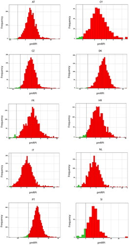
Table 4 shows the exposure statistics for the mean and high (P95) combined exposure. In the LB scenario, the mean combined exposure exceeded the ESRV of the reference compound cadmium by a factor 2.5 (Slovenia) to 3.7 (Austria and France). High combined exposure levels exceeded the ESRV of cadmium by a factor 4.5 (Slovenia) to 7.4 (France). For the UB scenario, 5.8 (Slovenia) to 8.3 (Austria) fold exceedance of the ESRV of cadmium was observed for the mean combined exposure. Ten to 14-fold exceedance of the ESRV of cadmium was found for the P95 combined exposure estimates.

Table 4. Classical modified reference point index (mRPI|) and personalised mRPI at mean and high (P95) exposure percentiles for metals relevant to kidney disease (lead, cadmium, inorganic arsenic and inorganic mercury) calculated for the adult population of ten European Countries.

	Classical mRPI				Personalised mRPI
	Mean^d		P95^d		Mean		P95
Country^a	LB^b	UB^c	LB	UB	LB	UB	LB	UB
AT	3.9 [3.0–4.4]	8.0 [6.5–9.5]	7.6 [5.2–11.6]	15.5 [12.4–20.7]	3.7 [3.1–4.3]	8.3 [7.5–9.2]	6.8 [5.5–9.0]	14.5 [12.4–16.9]
CY	2.8 [2.5–4.0]	6.8 [6.0–8.4]	6.7 [4.8–10.3]	13.3 [9.6–19.9]	2.9 [2.6–3.4]	6.7 [6.0–7.5]	5.8 [5.1–7.8]	12.2 [10.5–14.6]
CZ	3.0 [2.5–4.0]	6.3 [5.2–7.9]	6.1 [4.6–9.9]	12.1 [9.5–15.2]	3.2 [2.7–3.6]	6.6 [6.1–7.2]	6.0 [4.8–7.6]	11.4 [10.2–12.9]
DK	2.8 [2.3–3.6]	7.1 [5.2–8.8]	5.1 [3.8–7.6]	11.8 [8.7–15.4]	2.9 [2.5–3.4]	7.1 [6.8–8.0]	4.5 [3.8–6.0]	11.0 [9.5–12.8]
FR	3.6 [2.9–4.6]	7.9 [6.6–9.6]	8.0 [5.7–13.3]	15.2 [11.8–23.1]	3.6 [3.1–4.2]	7.6 [6.8–9.1]	7.4 [5.6–10.8]	13.6 [11.2–18.1]
HR	2.8 [2.0–3.3]	6.6 [5.5–7.7]	6.2 [4.2–10.1]	13.2 [10.3–18.9]	2.7 [2.4–3.2]	6.4 [5.8–7.3]	5.7 [4.4–8.2]	11.7 [9.9–15.0]
IT	3.5 [2.5–4.2]	7.8 [6.3–10.3]	6.0 [4.8–9.2]	14.5 [10.1–23.1]	3.5 [2.9–4.1]	7.9 [6.7–9.8]	6.3 [5.1–7.5]	14.0 [10.8–21.4]
NL	2.6 [2.0−3.6]	6.6 [5.8–8.5]	5.6 [3.7–7.1]	12.4 [9.5–17.2]	2.9 [2.5–3.3]	6.8 [6.1–7.9]	5.0 [4.3–5.7]	11.4 [9.7–14.0]
PT	2.9 [2.3–4.3]	7.1 [5.8–8.3]	7.0 [5.1–10.5]	13.8 [10.6–18.9]	3.2 [2.8–3.6]	7.0 [6.3–8.0]	6.2 [5.3–8.1]	12.6 [10.8–15.0]
SI	2.8 [1.8–3.6]	5.7 [4.6–7.7]	4.6 [3.4–7.3]	11.0 [7.8–17.0]	2.5 [2.0–3.3]	5.8 [4.8–7.1]	4.5 [3.4–5.5]	10.5 [8.2–14.0]

^a AT: Austria; CY: Cyprus; CZ: Czech Republic; DK: Denmark; FR: France; HR: Croatia; IT: Italy; NL: Netherlands; PT: Portugal; SI: Slovenia

^b LB is lower bound scenario. In this scenario analytical values below the limit of detection or limit of quantification were assumed to equal 0.

^c UB is upper bound scenario. In this scenario analytical values below the limit of detection or limit of quantification were assumed to equal the value of the respective limit.

^d Values between brackets indicate the upper and lower boundaries of the uncertainty interval quantified for uncertainties in food consumption and metal concentration data in food due limited sample sizes.

Table 4 also reports mRPIs obtained from the classical approach. For this, the exposure statistics for cadmium, lead, inorganic arsenic and inorganic mercury shown in Table 3 were divided by their respective ESRVs. Summing ERSV-adjusted mean exposures resulted in classical mRPIs ranging from 2.6 (the Netherlands) to 3.9 (Austria) in the LB scenario and from 5.7 (Slovenia) to 8.0 (Austria) in the UB scenario. Those values differed slightly from the personalised mRPI values. When ERSV-adjusted P95 exposures were summed, values obtained from the classical mRPI approach were about 10% higher than those obtained from the personalised mRPI approach. The classical mRPIs ranged from 4.6 (Slovenia) to 8.0 (France) in the LB scenario and from 11.0 (Slovenia) to 15.5 (Austria) in the UB scenario.

Risk driving chemicals

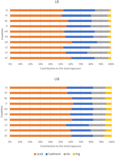
Figure 2 shows the contribution of each of the metals to the total combined exposure. Regardless the country or scenario, lead and cadmium together contributed around 80% to the total combined exposure. Lead was by far the major determinant of the total combined exposure; its contribution varied from 51 to 61% in the LB scenario (where measurements below the LOQ were assumed to be 0) and from 55 to 62% in the UB scenario (where measurements below the LOQ were assumed to equal the value of the LOQ). Cadmium contributed 21–31% to the total combined exposure in the LB scenario and 19–25% in the UB scenario. Inorganic arsenic impacted less on the total combined exposure (12–20% in the LB scenario; 11–16% in the UB scenario). Inorganic mercury only contributed marginally to the total combined exposure (4% or less in the LB scenario; 5–7% in the UB scenario).

Figure 2. Relative contribution of the individual metals to the personalised mRPI of metals relevant for chronic kidney disease. LB: Lower bound scenario in which values below the limit of quantification equalled 0. UB: Upper bound scenario in which values below the limit of quantification equalled the value of the limit of quantification. Pb: Lead; Cd: Cadmium; iA: inorganic arsenic; iHg: inorganic mercury; AT: Austria; CZ: Czech Republic; CY: Cyprus; DK: Denmark; Fr: France; HR: Croatia; IT: Italy; NL: the Netherlands; PT: Portugal; SI: Slovenia.

Risk-driving food-substance combinations

Figure 2 provides insight into risk-driving chemicals but information on risk-driving food-chemical combinations could provide additional information for risk managers to discuss legal maximum limits in food. Figure 3 gives information on the top 5 food-metal combinations that contributed most (i.e. 5% or more) to the total combined exposure per country, resulting in 13 food-metal combinations across countries. Lead in vegetables and products thereof and in grain and grain-based products contributed most to the personalised mRPI, regardless of the country and use of a lower versus UB scenario. For the other food-metal combinations per country results were more varied (Figure 3). In the LB scenario, cadmium in grain and grain-based products was an important determinant of the total combined exposure for most of the countries, while this combination was less important in the UB scenario.

Figure 3. Food-metal combination contributing 5% or more to the total combined exposure to metals relevant for chronic kidney disease. LB: Lower bound scenario in which values below the limit of quantification equalled 0. UB: Upper bound scenario in which values below the limit of quantification equalled the value of the limit of quantification. Pb: Lead; Cd: Cadmium; iAs: inorganic arsenic; iHg: inorganic mercury; AT: Austria; CZ: Czech Republic; CY: Cyprus; DK: Denmark; Fr: France; HR: Croatia; IT: Italy; NL: the Netherlands; PT: Portugal; SI: Slovenia.

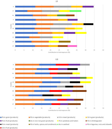
Depending on the scenario and country, lead in drinking water, meat and meat products, fruits and fruit products, herbs, spices and condiments, potatoes and other starchy roots and tubers, and legumes, nuts and oilseeds each contributed between 5 and 10% to the total combined exposure, as did cadmium in grain and grain-based products, fruit and fruit products, and meat and meat products. For inorganic arsenic, it was grain and grain-based products other than rice and/or fish and seafood that contributed 5–10% to the total combined exposure. There were no food products containing inorganic mercury that contributed 5% or more to the total combined exposure.

Discussion

Dietary exposure to single metals

In our case study, we used metal concentration data obtained from EFSA’s data warehouse for 14 European countries. It is therefore pertinent to compare our exposure estimates with those obtained by EFSA in their most recent assessments. As EFSA only assessed the exposure to single metals, we also assessed the exposure to those single metals. Cadmium, lead and LB inorganic mercury exposure estimates in our case study differed only slightly from those published in the most recent EFSA opinions (Table 3; EFSA (2012b, 2012a, 2012c, 2021a)). Somewhat larger deviations from EFSA estimates were observed for inorganic arsenic (on average 4.5 times higher than the mean exposure calculated by EFSA (2021a)) and UB inorganic mercury exposure (approximately 2.5 times higher than the most recent EFSA assessment (EFSA 2012c)). Differences could be due to differences in food consumption data (more recent surveys in our assessment), metal concentration data (less data because of fewer countries and more recent data in our assessment) and the linkage of food consumption data to metal concentration data (use of Dutch recipes in our assessment). The use of EFSA’s raw primary commodity model, which transforms food consumption data into raw primary commodity consumption data for each country in the EFSA data warehouse and takes into account variability in recipes (Dujardin and Kirwan 2019) can overcome the uncertainty in food recipes. Currently, EFSA’s raw primary commodity model is, however, not compatible with the FoodEx classification system as it focuses on the nomenclature used in the pesticide framework.

Regarding inorganic arsenic, the same food consumption data and concentration data over the same time period were used as compared to the EFSA assessment (EFSA 2021a). However, higher mean concentrations were observed in bread and rolls, cereal flakes, biscuit and cookies, fish meat, prawns, water molluscs, dietary supplements, meat-based meals and prepared mixed vegetable salads. These higher mean concentrations of inorganic arsenic in non-seafood products could be due to unintentional oversampling of rice-based products in foods aggregated to a non-specific food category (such as cereal flakes) for which no additional data on the source of cereals was available in our study. In addition, for fish meat, prawns and water molluscs, we used conversion factors to calculate inorganic arsenic from total arsenic. Considerable uncertainty was introduced when predicting inorganic arsenic concentrations out of total arsenic in seafood, as the relative proportion of inorganic arsenic tends to decrease as the total arsenic content increases. Moreover, this varies depending on the seafood species (EFSA 2009b, Supplemental Material A). Therefore, the use of conversion factors could have led to an overestimation of the exposure to inorganic arsenic. Using conservative conversion factors to calculate inorganic mercury concentrations from total mercury could also have overestimated the exposure to inorganic mercury (EFSA 2012c). The direct chemical analysis of inorganic metals in more (types of) food products, as recommended by EFSA in their opinions (EFSA 2012c, 2021a) will reduce this uncertainty.

Single metal risk assessment is usually based on the critical effect of the metal, i.e. the toxic effect observed at the lowest exposed dose of a chemical. CKD is the critical effect for cadmium, lead and inorganic mercury (EFSA 2009a, 2010b; JECFA 2011; EFSA 2012c) but not for inorganic arsenic (EFSA 2009b), for which carcinogenic effects were considered critical. Our MRA focussed on the common effect of four metals on kidney function. Therefore, the comparison of the dietary exposure to single metals in our study with those published by EFSA is restricted to three (cadmium, lead and inorganic mercury) out of four metals. For cadmium, the EFSA TWI of 2.5 µg/kg bw/d (EFSA 2009a) was divided by 7 to obtain the ESRV of 0.36 µg/kg bw/d. Like EFSA’s risk assessment (EFSA 2012a) exceedances of this value were observed (Table 3), particularly for the high exposure percentiles.

For lead, EFSA used the BMDL₁₀ of 0.63 µg/kg bw/d for effects on the glomerular filtration rate in a margin of exposure approach but did not state clearly which margin of exposure would be tolerable (EFSA 2010b). EFSA concluded that a margin of exposure of at least 10 would be sufficient to ensure that there was no appreciable risk of a clinically significant change in the prevalence of CKD. EFSA also stated that at a margin of exposure greater than 1, the risk would be very low. In their most recent exposure assessment, EFSA compared the lead exposure directly to the BMDL₁₀, which suggests that a margin of exposure of 1 would be tolerable (EFSA 2012b). In our study, we used an UF of 3.16 for differences in toxicodynamics because the elderly, who are the most sensitive population for CKD, were underrepresented in the epidemiological cohort. This resulted in an ESRV of 0.2 µg/kg bw/d. Mean and high exposure exceeded this ESRV in all populations (Table 3).

For inorganic mercury, EFSA derived a TWI of 4.0 µg inorganic mercury/kg bw, expressed as mercury (EFSA 2012c), which was based on kidney weight changes in rats. As it remains unclear how kidney weight changes in rats relate to glomerular or tubular effects in humans, we selected the point of departure based on tubular/glomerular effects in humans (Table 1). When the EFSA TWI is divided by 7, a daily dose of 0.57 µg/kg bw is obtained, which is somewhat lower than the ESRV of 0.75 µg/kg bw/d. Dietary exposure to inorganic mercury did not exceed this value (Table 3) nor the EFSA TWI, as was shown in EFSA’s risk assessment (EFSA 2012c).

Combined dietary exposure to the four metals

The dietary exposure assessment to single metals showed that exposure to cadmium or lead alone may already result in exceeding tolerable intake levels for CKD. Thus, a combined exposure to cadmium, lead and also the other nephrotoxic metals will result in an even larger exceedance of tolerable intake levels. To assess the combined exposure to the four metals, we used the classical and personalised mRPI approach. The mRPI reflects the fold-exceedance of the tolerable dose of, in our study, cadmium used as a reference compound. The personalised mRPI approach expresses the exposure to metals as equivalents of cadmium for each individual in the food consumption database, and relates those cadmium-equivalents to the ESRV of cadmium. This results in a distribution of individual mRPIs, from which exposure statistics were obtained. This personalised mRPI approach provides a more realistic assessment than classical approaches relying on summary statistics of exposures at the median or the P95 (see e.g. (Evans et al. 2016; Martin et al. 2017; EFSA 2019; Vejdovszky et al. 2019; Sprong et al. 2020; Boberg et al. 2021) as illustrated by van den Brand et al. (2022) and by Kortenkamp et al. (2022)). The use of summarised population statistics does not allow for dealing with the fact that individuals that are highly exposed to one chemical may not necessarily be highly exposed to another substance. This way of combining exposures can as such be considered a ‘worst-case’ scenario. For example, a high exposure to lead due to a high consumption of grain-based products, fruit and vegetables does not necessarily coincide with high exposure to inorganic arsenic due to a high consumption of seafood. Summing exposure equivalents derived from high exposure percentiles is, therefore, considered as conservative. Our results, however, showed that personalised mRPIs obtained for the upper exposure levels (P95) were about 10% lower than those obtained from the classical approach (Table 4). This is probably due to the fact that cadmium and lead, which together contributes to about 80% of the combined exposure, often were present in the same foods (Supplemental Material A), including frequently consumed foods like grains, vegetables and fruit. Other case studies with different classes of chemicals may show greater divergence between the upper exposure levels, emphasising the conservative nature of the classical mRPI approach resulting from summing the statistics per individual chemical. Regardless the approach taken median and high exposure assessment exceeded the tolerable dose of cadmium. Exceedances were up to 2.5–14 times in the personalised mRPI approach depending on the exposure statistic (median or P95), scenario (LB or UB) or country (Table 4).

It should be noted that individual ESRV values for cadmium and lead are exceeded in many countries (Table 3). If cadmium and lead exposures were compliant with the respective ESRVs in those countries, the mRPI would be at least two. Given the fact that the ESRVs for cadmium and lead are based on the critical effect and thus used for risk assessment of exposure to the single metals, this could indicate that toxicological reference values deemed tolerable for exposure to single metals might not be protective for combined exposure to metals if exposures are around this value. However, uncertainties in the ESRVs (see Uncertainties in hazard data section) introduced uncertainties in summing the risk and those should be addressed first before drawing conclusions on the protectiveness of toxicological reference values used for single risk assessment for combined exposure to metals.

In this assessment, only dietary exposure to the metals was considered, thus neglecting other relevant routes of exposure, such as air, cigarette smoke, dust and soil. Smoking cigarettes may contribute 15–30% to the total cadmium exposure (EFSA 2009a), and up to 5% to the total lead exposure (EFSA 2010b). Regarding non-smokers, the contribution of non-dietary sources to the overall exposure of adults in the general population is relatively low: for cadmium up to 20%, for lead up to 10% and for inorganic arsenic up to 1% in non-smoking subjects (EFSA 2009a, 2009b, 2010b). Dental amalgam and thiomersal used as a preservative in vaccines and some personal care products could contribute to inorganic mercury exposure (EFSA 2012c). Occupational exposure of workers to metals could cause additional exposure via other routes. Most likely neglecting other sources of metal exposure will have resulted in an underestimation of the true combined exposure to metals.

Human biomonitoring data can be used to assess the combined exposure to multiple chemicals from all sources (Luijten et al. 2023). While less refined methods are available to cumulate the risk (e.g. Socianu et al. 2022) based on human biomonitoring data, further refined methods, such as the personalised mRPI approach are still in their infancy. Such refined methods could be considered by risk assessors in the future. Although human biomonitoring integrates the individual’s exposure from all sources and exposure routes and could provide information on metals contributing most to the exposure or risk, it is more difficult to assign risk-driving sources of exposure. Yet for addressing risk management questions, this information is required. External exposure assessment, like our dietary exposure assessment, does provide information on risk driving-sources. Our case study showed that grains and grain-based products were important contributors to the combined risk of cadmium and lead, as were cadmium and lead in meat and meat products. Also, lead in vegetables and vegetable products, drinking water, fruits and fruit products, herbs, spices and condiment, potatoes and other starchy roots and tubers and legumes, nuts and oil seeds contributed considerably to the exposure. Furthermore, inorganic arsenic in non-rice grains and grain-based products and fish and seafoods impacted on the exposure. Risk managers may consider revising existing maximum limits for food in the EU as laid down in Regulation 1881/2006 (EC 2006) and for drinking water in Directive 2020/2184 (EC 2020), or they may consider setting additional maximum limits on metal concentrations in foods that are not included in Regulation 1881/2006. As many healthy foods, such as vegetables, fruit, whole grains, legumes and nuts contain (low) concentrations of metals, a risk-benefit analysis for the combined exposure to metals could be considered, as has been performed for the individual metals, such as the presence of methyl mercury and beneficial fatty acids in fish (FAO/WHO 2011).

In this work, the MRA was restricted to the four metals only. It should be noted that people are exposed to other nephrotoxic substances as well. Vejdovszky et al. (2021) performed an mPRI approach for lead, cadmium, 3-monochloropropane-1,2-diol (renal tubular hyperplasia), fumonisins B1, B2 and B3 (nephrotoxicity), methyl mercury (CKD), ochratoxin A (altered kidney enzymes) and patulin (altered kidney function). Lead and cadmium contributed 77% to the combined exposure, comparable to this study, where both metals contributed up to 80% to the combined exposure. Neglecting these other substances in a risk assessment has underestimated the combined risk of nephrotoxicity at the organ level. Yet, further refinement of the assessment to a higher tier, where only chemicals with the same mode of action are grouped together, may result in a significantly lower risk estimate.

Uncertainties

As for all risk assessments, the one performed in our case study involves uncertainties in the exposure and hazard data used. Identification of those uncertainties is needed to assess whether the assessment represents an overestimation or an underestimation of risks. If possible expert knowledge elicitation and probabilistic modelling could be performed to integrate complex uncertainty patterns into an overall uncertainty estimate (EFSA 2014, 2020a, 2020b). Expert knowledge elicitation is a resource-intensive exercise that could not be performed within the budget of the project. Instead, a description of the identified uncertainties is described below. Where known, the direction of the uncertainty (overestimation or underestimation) was provided.

Uncertainties in exposure data

Uncertainties in exposure data are related to food consumption data, metal concentration data and matching food consumption data to metal concentration data. Sampling uncertainty in food and consumption data caused by the limited sampling size was assessed using the bootstrap approach (Efron 1979; Efron and Tibshirani 1993), which resulted in an uncertainty interval around the exposure estimates (Tables 3 and 4). This uncertainty interval indicates what the exposure estimate could have been if other samples from the population and foods were used, assuming that representative sampling was applied. Sampling uncertainty did not affect the outcome of the MRA since none of the LBs of the uncertainty interval around the personalised mRPI is smaller than 1.

The uncertainty caused by measurements below the LOQ was addressed by the lower and UB scenarios where those samples were substituted by zero or the value of the LOQ, respectively. The LB scenario reflects an underestimate of the exposure while the UB scenario overestimates the exposure. These scenarios are frequently performed in exposure assessments. If the LB scenario indicates that exposure does not exceed the limit that is currently considered tolerable while exposure in the UB does exceed those limits, refinement of the concentration data could be useful to gain insight on the most realistic exposure. In our case study, both the lower and UB scenario resulted in an exposure exceeding the limit that is currently considered tolerable. Therefore, refinement of LOQs (i.e. lower LOQs) would not improve the exposure assessment.

Several other sources of uncertainties could not be quantified in our assessment. A detailed description of general uncertainties in dietary exposure and more specific for lead and inorganic arsenic exposure has been recently described by Sprong et al. (2023), which used the same food consumption data, concentration data (for lead and inorganic arsenic) and Dutch recipes for matching food consumption data to concentration data in a case study on MRA for chemicals relevant for cognitive decline in children. Uncertainties included the use of the food coding system and assumptions made to handle data gaps, such as the use of a conversion factor (as already described for inorganic arsenic and inorganic mercury in section ‘Dietary exposure to single metals’) and aggregation of foods to a higher FoodEx1 hierarchy for foods with fewer than 50 measurements. For inorganic mercury and cadmium, the same uncertainties are applicable. In many cases, the direction of the uncertainty was undefined.

Uncertainties in hazard data

MRA is preferably conducted using relative potency factors (RPFs) for components of a mixture to express exposure as equivalents of the reference compound (e.g. cadmium in our case study) to combine the exposure. Such RPFs can be obtained only if the different components of the mixture under study 1) act via a common mode of action; 2) differ only in potency (i.e. their individual dose–response curves should be parallel on log–dose scale), 3) do not interact (Bosgra et al. 2009; EFSA 2019; Bil et al. 2023), and 4) if dose-response relationships between contributing substances and a common adverse effect are determined in one study (in one matrix) or using different studies with the same study design. Since this information is lacking for the metals in our case study, we used the personalised mRPI approach, which is less restrictive in its assumptions as it only requires reference points and UFs for a common endpoint (Vejdovszky et al. 2019), such as CKD. However, this approach may have introduced some uncertainties in the MRA of dietary exposure to the four metals, as it unclear how a BMDL₀₅ for elevated beta-2 microglobulin excretion in humans relates to a BMDL₁₀ for a reduced glomular filtration rate, and a NOAEL for increased levels of retinol-binding protein. Recently, an AOP for the four metals has been developed for proximal tubular damage (Sarigiannis 2022). This AOP can be used to identify (novel) effect biomarkers for which simultaneous benchmark modelling could be performed to obtain RPFs for higher tier MRA.

The choices and assumptions made for ESRVs in the mRPI approach may have affected the outcome of our study. Uncertainties in reference points, kinetic modelling from internal concentrations to external dietary sources and selection of uncertainty factors may have influenced the value of the ESRV and hence the personalised mRPI.

For cadmium, the ESRV was obtained by dividing the EFSA TWI of 2.5 µg cadmium/kg bw (EFSA 2009a, 2009b) to obtain a daily dose of 0.36 µg cadmium/kg bw. EFSA based their TWI on a dose-response relationship between urinary cadmium and elevated beta-2-microglobulin (a biomarker for tubular effects) levels observed in a meta-analysis using group means of human cohorts and derived a urinary BMDL₀₅ of 4 µg cadmium/g creatinine. Like EFSA, we applied a chemical-specific adjustment factor of 3.9, to account for uncertainty generated by using group means instead of data points from individual subjects, which resulted in a value of 1.0 µg Cd/g creatinine. The chemical-specific adjustment factor was defined as the ratio of the 95th population percentile to the median BMD and was included to cover 95% of the population (EFSA 2009a). Recently, the value of 1.0 µg cadmium/g creatinine was proposed as a human biomonitoring guidance value for the general population (Lamkarkach et al. 2021). EFSA modelled the urinary BMDL₀₅ into an external dietary dose using kinetic modelling assuming an absorbed fraction of 10% (Amzal et al. 2009), i.e. the highest fraction observed in human adults (men 5% and women 10%) (EFSA 2009a).

Regarding lead, ECHA listed several blood reference points for effects on CKD in lead-exposed workers in their evaluation of limit values for lead and its compounds at the workplace (ECHA 2020). Those BMDLs were much higher than the BMDL₁₀ of 15 µg/L blood in our case, e.g. a BMDL₀₅ of 101 µg/L urine and a BMDL₁₀ of 253 µg/L urine for changes in urinary excretion of N-acetyl-β-D-glucosaminidase (NAG; a biomarker of tubular effects) were calculated for storage battery workers (Lin T and Tai-yi 2007; Sun et al. 2008) and a BMDL₁₀ of 402 µg/L blood was obtained for urinary total protein in storage battery workers (Lin T and Tai-yi 2007). According to ECHA, the BMDL₁₀ value of 253 µg/L urine for sub-clinical changes from an effect marker of renal impairment (NAG) could be considered the NOAEL. It should be noted that changes in urinary excretion of NAG were considered by ECHA as sub-clinical and their long-term prognostic value is unclear, and therefore changes in NAG cannot be considered as adverse (ECHA 2020). A disadvantage of extrapolating reference points of metals in workers is the intermittent (relatively high) exposure (e.g. 8 h/d, 40 h/week), compared with more chronic (relatively low) exposure via food and drinking water. The different BMDLs indicate that uncertainty still exists around the ESRV and the preferred human biomonitoring matrix for lead.

For inorganic arsenic, we used the BMDL₁₀ derived by Lin et al. (2020). It should be noted that exposure to other metals could have biased this reference point, as those authors did not correct the BMD analysis for other confounding metals, such as cadmium or lead levels. This could have resulted in an overestimation of the risk of inorganic arsenic.

Several points of departure were available for the nephrotoxic effects of inorganic mercury (SCOEL 2007; EFSA 2012c). As we were interested in tubular or glomerular effects, we used the urinary NOAEL of 35 µg inorganic mercury/g creatinine, which was based on the absence of increased enzyme (galactosidase) excretion in workers. Using a simple kinetic equation (Equation (1)(1) $$D_{\mathit{dietary}}=\mathrm{ }\frac{\mathrm{C}c\mathrm{\hspace{0.17em}*\hspace{0.17em}}{C}_e}{F_a\mathrm{\hspace{0.17em}*\hspace{0.17em}}{F}_{\mathit{u}\mathit{e}}\mathrm{\hspace{0.17em}*\hspace{0.17em}}bw}$$(1) ) and assumptions for C_e (1.5 g/d; Hays et al. 2010), F_a (0.1; the highest of a range reported for humans by JECFA (2011)), F_ue (1; all absorbed inorganic mercury excreted in urine), a mean bodyweight of 70 kg, and an additional UF of 10, we obtained an ESRV of 0.75 µg/kg bw/d. When multiplied by 7, a weekly dose of 5.3 µg/kg bw was obtained, which is slightly higher than the EFSA TWI of 4 µg inorganic mercury/kg bw, expressed as mercury. EFSA based their TWI on kidney weight changes in rats, and not on the data from several epidemiological studies showing nephrotoxic effects of inorganic mercury. This is because EFSA’s CONTAM panel concluded that the epidemiological studies suffered from several limitations, such as a small study group, insufficient control for confounders, inadequate exposure assessment, and insufficient differentiation between mercury compounds and routes of exposure (EFSA 2012c). Our results show that the ESRV based on a NOAEL of 35 µg mercury/g creatinine that was identified by SCOEL (2007), closely resembles EFSA’s health-based guidance value.

Based on the study of Roels et al. (1985), the SCOEL also derived an lowest observed adverse effect level of 50 µg inorganic mercury/g creatinine for increased protein excretion in workers (SCOEL 2007). Using the same model and assumptions as described above for the NOAEL of 35 mercury/g creatinine would have resulted in an ESRV of 1 µg/kg bw/d. Since the ESRV of 0.75 µg inorganic mercury/kg bw/d used in our study is more conservative, we selected this one in our assessment. Other proposed human biomonitoring health-based guidance values were not deemed relevant as they were based on other endpoints, such as the biological limit values of 10 µg/L blood and 30 µg/g creatinine set by the SCOEL, as those relates to neurological effects (Roels et al. 1985; SCOEL 2007).

Taken together, the personalised mRPI approach in our study was performed with the ESRVs currently available. If future studies provide RPFs or better ESRVs as input in a personalised mRPI approach, a new assessment could be performed.

Conclusion

This case study shows that dietary exposure of adults to cadmium alone may already exceed the tolerable intake level. The same holds true for dietary exposure to lead only. When the exposure to cadmium, lead, inorganic arsenic and inorganic mercury was combined in a component-based approach using the personalised mRPI methodology, the combined exposure exceeded the tolerable level 2–14 times in 10 European countries, depending on the exposure statistics, the exposure scenario and the country. The methodology provides useful information for risk managers on exceedances of the tolerable combined exposures and on sources of exposure, which could feed into re-evaluations of legal limits of substances in food and dietary recommendations to the population. As expected from the single metal assessments, cadmium and lead contributed strongly to the personalised mPRI, followed by inorganic arsenic. The impact of inorganic mercury on the personalised mRPI was limited, due to its low exposure compared to the other substances and a (relatively) higher ESRV. In our case study, lead and cadmium in grains and meat were important contributors to the combined risk. Lead in vegetables, dairy, drinking water, fruits, herbs, spices and condiments, starchy roots and tubers also contributed importantly to the combined exposure. Regarding inorganic arsenic, non-rice grains, fish and seafoods and/or composite foods impacted on the total combined exposure. There were no food products containing inorganic mercury that contributed 5% or more to the total combined exposure. Uncertainties were identified in exposure data (such as conversion factors for total arsenic and mercury to the inorganic forms) and hazard data (differences in principles in the derivation of reference points). Yet, MRA at the target organ level as performed in our study could be regarded as a way to prioritise assessment groups for higher-tier MRA. Since the combined exposure to the four metals exceeded the tolerable level of cadmium considerably, a refined MRA based on a common specific nephrotoxic effect could be the next step.

Abbreviations
BMD	=	benchmark dose
BMDLx	=	benchmark dose lower limit, related to a x% change in response
CKD	=	chronic kidney disease
ECHA	=	European Chemicals Agency
EFSA	=	European Food Safety Authority
ESRV	=	endpoint specific reference value
JECFA	=	Joint FAO/WHO Expert Committee on Food Additives
LB	=	lower bound scenario
LOD	=	limit of detection
LOQ	=	limit of quantification
MCRA	=	Monte Carlo Risk Assessment
MRA	=	mixture risk assessment mRP I-modified reference point index
NAG	=	N-acetyl-β-Dglucosaminidase
NOAEL	=	no observed adverse effect level
P95	=	95th percentile RP Fs-relative potency factors
SCOEL	=	Scientific Committee on Occupational Exposure Limits
TWI	=	tolerable weekly intake
UB	=	upper bound scenario
UF	=	uncertainty factor

Acknowledgements

The authors would like to thank Matthijs Sam (RIVM) for his help in organising the food consumption data and chemical concentration data, Jan Dirk Te Biesebeek (RIVM) for his help with the exposure assessment, EFSA for providing the food consumption databases, and data owners for giving permission to use the data.

Disclosure statement

The authors report there are no competing interests to declare.

Additional information

Funding

The work performed for this article started in the HBM4EU project which received funding from the European Union’s Horizon 2020 research and innovation program under Grant Agreement No. 733032 (ADvdB, GvD, ERG, ML and MJBM) and was completed in the framework of the European Partnership for the Assessment of Risks from Chemicals (PARC) which received funding from the European Union’s Horizon Europe Research and Innovation Programme under Grant Agreement No. 101057014 (RCS, AC, AM and JDvK) and Horizon 2020 Framework Programme.

References

- Amzal B, Julin B, Vahter M, Wolk A, Johanson G, Akesson A. 2009. Population toxicokinetic modeling of cadmium for health risk assessment. Environ Health Perspect. 117(8):1293–1301. doi: 10.1289/ehp.0800317.
- Berglund M, Lind B, Bjornberg KA, Palm B, Einarsson O, Vahter M. 2005. Inter-individual variations of human mercury exposure biomarkers: a cross-sectional assessment. Environ Health. 4(1):20. doi: 10.1186/1476-069X-4-20.
- Bil W, Ehrlich V, Chen G, Vandebriel R, Zeilmaker M, Luijten M, Uhl M, Marx-Stoelting P, Halldorsson TI, Bokkers B. 2023. Internal relative potency factors based on immunotoxicity for the risk assessment of mixtures of per- and polyfluoroalkyl substances (PFAS) in human biomonitoring. Environ Int. 171:107727. doi: 10.1016/j.envint.2022.107727.
- Boberg J, Bredsdorff L, Petersen A, Lobl N, Jensen BH, Vinggaard AM, Nielsen E. 2021. Chemical mixture calculator - A novel tool for mixture risk assessment. Food Chem Toxicol. 152:112167. doi: 10.1016/j.fct.2021.112167.
- Boobis AR, Ossendorp BC, Banasiak U, Hamey PY, Sebestyen I, Moretto A. 2008. Cumulative risk assessment of pesticide residues in food. Toxicol Lett. 180(2):137–150. doi: 10.1016/j.toxlet.2008.06.004.
- Boon PE, van Donkersgoed G, Christodoulou D, Crépet A, D'Addezio L, Desvignes V, Ericsson B-G, Galimberti F, Ioannou-Kakouri E, Jensen BH, et al. 2015. Cumulative dietary exposure to a selected group of pesticides of the triazole group in different European countries according to the EFSA guidance on probabilistic modelling. Food Chem Toxicol. 79:13–31. doi: 10.1016/j.fct.2014.08.004.
- Bopp SK, Barouki R, Brack W, Dalla Costa S, Dorne JCM, Drakvik PE, Faust M, Karjalainen TK, Kephalopoulos S, van Klaveren J, et al. 2018. Current EU research activities on combined exposure to multiple chemicals. Environ Int. 120:544–562. doi: 10.1016/j.envint.2018.07.037.
- Bosgra S, van der Voet H, Boon PE, Slob W. 2009. An integrated probabilistic framework for cumulative risk assessment of common mechanism chemicals in food: an example with organophosphorus pesticides. Regul Toxicol Pharmacol. 54(2):124–133. doi: 10.1016/j.yrtph.2009.03.004.
- Buchet JP, Roels H, Bernard A, Lauwerys R. 1980. Assessment of renal function of workers exposed to inorganic lead, calcium or mercury vapor. J Occup Med. 22(11):741–750.
- Carlisle JC, Wade MJ. 1992. Predicting blood lead concentrations from environmental concentrations. Regul Toxicol Pharmacol. 16(3):280–289. doi: 10.1016/0273-2300(92)90008-w.
- Dujardin B, Kirwan L. 2019. The raw primary commodity (RPC) model: strengthening EFSA’s capacity to assess dietary exposure at different levels of the food chain, from raw primary commodities to foods as consumed. EFSA Supporting publication 2019: EN-1532.
- European Commission (EC). 2006. COMMISSION REGULATION (EC) No 1881/2006 of 19 December 2006 setting maximum levels for certain contaminants in foodstuffs. J Eur Union L. 364:5–24.
- European Commission (EC). 2020. Directive (EU) 2020/2184 of the European parliament and of the council of 16 December 2020 on the quality of water intended for human consumption (recast). J Eur Union L. 345:1–62.
- European Chemicals Agency (ECHA). 2020. ECHA Scientific report for evaluation of limit values for lead and its compounds at the workplace. Helsinki, Finland.
- Efron B. 1979. Bootstrap methods: another look at the jackknife. Ann Statist. 7(1):1–26. doi: 10.1214/aos/1176344552.
- Efron B, Tibshirani RJ. 1993. An introduction to the bootstrap. New York (NY): Chapman & Hall.
- European Food Safety Authority (EFSA). 2009a. Cadmium in food. EFSA J. 980:1–139.
- European Food Safety Authority (EFSA). 2009b. Scientific opinion on arsenic in food. EFSA J. 7(10):1351.
- European Food Safety Authority (EFSA). 2010a. Management of left-censored data in dietary exposure assessment of chemical substances. EFSA J. 8(3):1557.
- European Food Safety Authority (EFSA). 2010b. Scientific opinion on lead in food. EFSA J. 8(8):1570.
- European Food Safety Authority (EFSA). 2010c. Standard sample description for food and feed. EFSA J. 8(1):1457.
- European Food Safety Authority (EFSA). 2011. Evaluation of the FoodEx, the food classification system applied to the development of the EFSA comprehensive European food consumption database. EFSA J. 9(3):1970.
- European Food Safety Authority (EFSA). 2012a. Cadmium dietary exposure in the European population. EFSA J. 10(1):2551.
- European Food Safety Authority (EFSA). 2012b. Lead dietary exposure in the European population1. EFSA J. 10(7):2831.
- European Food Safety Authority (EFSA). 2012c. Scientific opinion on the risk for public health related to the presence of mercury and methylmercury in food. EFSA J. 10(12):1–241.
- European Food Safety Authority (EFSA). 2014. Guidance on expert knowledge elicitation in food and feed safety risk assessment. EFSA J. 12(6):3734.
- European Food Safety Authority (EFSA). 2019. Guidance on harmonised methodologies for human health, animal health and ecological risk assessment of combined exposure to multiple chemicals. EFSA J. 17(3):e05634.
- European Food Safety Authority (EFSA). 2020a. Cumulative dietary risk characterisation of pesticides that have acute effects on the nervous system. EFSA J. 18(4):e06087.
- European Food Safety Authority (EFSA). 2020b. Cumulative dietary risk characterisation of pesticides that have chronic effects on the thyroid. EFSA J. 18(4):e06088.
- European Food Safety Authority (EFSA). 2021a. Chronic dietary exposure to inorganic arsenic. EFSA J. 19(1):e06380.
- European Food Safety Authority (EFSA). 2021b. Guidance document on scientific criteria for grouping chemicals into assessment groups for human risk assessment of combined exposure to multiple chemicals. EFSA J. 19(12):e07033.
- Evans RM, Martin OV, Faust M, Kortenkamp A. 2016. Should the scope of human mixture risk assessment span legislative/regulatory silos for chemicals? Sci Total Environ. 543(Pt A):757–764. doi: 10.1016/j.scitotenv.2015.10.162.
- Food and Agricultural Organization of the United Nations (FAO)/World Health Organisation (WHO). 2011. Joint FAO/WHO expert consultation on the risks and benefits of fish consumption. Rome: Food and Agricultural Organization of the United Nations; Geneva: World Health Organization; p. 50.
- Foa V, Colombi A, Maroni M, Buratti M, Calzaferri G. 1984. The speciation of the chemical forms of arsenic in the biological monitoring of exposure to inorganic arsenic. Sci Total Environ. 34(3):241–259. doi: 10.1016/0048-9697(84)90066-4.
- Fox MA, Brewer LE, Martin L. 2017. An overview of literature topics related to current concepts, methods, tools, and applications for cumulative risk assessment (2007–2016). Int J Environ Res Public Health. 14(4):389.
- Hays SM, Aylward LL, Gagne M, Nong A, Krishnan K. 2010. Biomonitoring equivalents for inorganic arsenic. Regul Toxicol Pharmacol. 58(1):1–9. doi: 10.1016/j.yrtph.2010.06.002.
- Hong F, Jin T, Zhang A. 2004. Risk assessment on renal dysfunction caused by co-exposure to arsenic and cadmium using benchmark dose calculation in a Chinese population. Biometals. 17(5):573–580. doi: 10.1023/b:biom.0000045741.22924.d8.
- International Program in Chemical Safety (ICPS). 2020. Dietary exposure assessment for chemicals in food. Environmental health criteria 240: principles and methods for the risk assessment of chemicals in food. Rome: Food and Agriculture Organization of the United Nations; Geneva: World Health Organization.
- Joint Food and Agricultural Organization of the United Nations (FAO)/World Health Organization (WHO) Expert Committee on Food Additives (JECFA). 2011. Safety evaluation of certain contaminants in food. Mercury (addendum). Evaluation of certain contaminants in food: seventy-second report of the Joint FAO/WHO Expert Committee on Food Additives. WHO Technical Report Series No. 959. Rome: Food and Agricultural Organization of the United Nations; Geneva: World Health Organization.
- Kortenkamp A, Scholze M, Ermler S, Priskorn L, Jorgensen N, Andersson AM, Frederiksen H. 2022. Combined exposures to bisphenols, polychlorinated dioxins, paracetamol, and phthalates as drivers of deteriorating semen quality. Environ Int. 165:107322. doi: 10.1016/j.envint.2022.107322.
- Lamkarkach F, Ougier E, Garnier R, Viau C, Kolossa-Gehring M, Lange R, Apel P. 2021. Human biomonitoring initiative (HBM4EU): human biomonitoring guidance values (HBM-GVs) derived for cadmium and its compounds. Environ Int. 147:106337. doi: 10.1016/j.envint.2020.106337.
- Lin T, Tai-Yi J. 2007. Benchmark dose approach for renal dysfunction in workers exposed to lead. Environ Toxicol. 22(3):229–233. doi: 10.1002/tox.20260.
- Lin YJ, Hsiao JL, Hsu HT. 2020. Integration of biomonitoring data and reverse dosimetry modeling to assess population risks of arsenic-induced chronic kidney disease and urinary cancer. Ecotoxicol Environ Saf. 206:111212. doi: 10.1016/j.ecoenv.2020.111212.
- Luijten M, Vlaanderen J, Kortenkamp A, Antignac JP, Barouki R, Bil W, van den Brand A, den Braver-Sewradj S, van Klaveren J, Mengelers M, et al. 2023. Mixture risk assessment and human biomonitoring: lessons learnt from HBM4EU. Int J Hyg Environ Health. 249:114135. doi: 10.1016/j.ijheh.2023.114135.
- Martin OV, Evans RM, Faust M, Kortenkamp A. 2017. A human mixture risk assessment for neurodevelopmental toxicity associated with polybrominated diphenyl ethers used as flame retardants. Environ Health Perspect. 125(8):087016. doi: 10.1289/EHP826.
- Organisation for Economic Co-operation and Development (OECD). 2018. Considerations for assessing the risk of combined exposure to multiple chemicals. Series on testing and assessment No. 296, Environment, Health and Safety Division, Environment Directorate, Paris, France.
- Roels H, Gennart JP, Lauwerys R, Buchet JP, Malchaire J, Bernard A. 1985. Surveillance of workers exposed to mercury vapour: validation of a previously proposed biological threshold limit value for mercury concentration in urine. Am J Ind Med. 7(1):45–71. doi: 10.1002/ajim.4700070106.
- Rotter S, Beronius A, Boobis AR, Hanberg A, van Klaveren J, Luijten M, Machera K, Nikolopoulou D, van der Voet H, Zilliacus J, et al. 2018. Overview on legislation and scientific approaches for risk assessment of combined exposure to multiple chemicals: the potential EuroMix contribution. Crit Rev Toxicol. 48(9):796–814. doi: 10.1080/10408444.2018.1541964.
- Sarigiannis D. 2022. Final report on AOPs. Deliverable Report D13.6; HBM4EU. https://www.hbm4eu.eu/work-packages/deliverable-13-6-final-report-on-aops/.
- Scientific Committee on Occupational Exposure Limits (SCOEL) of the European Commission. 2007. Recommendation from the scientific committee on occupational exposure limits for elemental mercury and inorganic divalent mercury compounds. https://echa.europa.eu/recommendations-of-the-scoel.
- Socianu S, Bopp SK, Govarts E, Gilles L, Buekers J, Kolossa-Gehring M, Backhaus T, Franco A. 2022. Chemical mixtures in the EU population: composition and potential risks. Int J Environ Res Public Health. 19(10):6121.
- Sprong C, Crepet A, Metruccio F, Blaznik U, Anagnostopoulos C, Christodoulou DL, Jensen BH, Kennedy M, Gonzalez N, Rehurkova I, et al. 2020. Cumulative dietary risk assessment overarching different regulatory silos using a margin of exposure approach: a case study with three chemical silos. Food Chem Toxicol. 142:111416. doi: 10.1016/j.fct.2020.111416.
- Sprong C, Te Biesebeek JD, Chatterjee M, Wolterink G, van den Brand A, Blaznik U, Christodoulou D, Crépet A, Hamborg Jensen B, Sokolić D, et al. 2023. A case study of neurodevelopmental risks from combined exposures to lead, methyl-mercury, inorganic arsenic, polychlorinated biphenyls, polybrominated diphenyl ethers and fluoride. Int J Hyg Environ Health. 251:114167.
- Sun Y, Sun D, Zhou Z, Zhu G, Lei L, Zhang H, Chang X, Jin T. 2008. Estimation of benchmark dose for bone damage and renal dysfunction in a Chinese male population occupationally exposed to lead. Ann Occup Hyg. 52(6):527–533.
- Te Biesebeek JD, Sam M, Sprong RC, van Donkersgoed G, Kruisselbrink JW, de Boer WJ, van Lenthe M, van der Voet H, van Klaveren JD. 2021. Potential impact of prioritisation methods on the outcome of cumulative exposure assessments of pesticides. EFSA Support Public. EN(6559):99.
- van den Brand AD, Bokkers BGH, Te Biesebeek JD, Mengelers MJB. 2022. Combined exposure to multiple mycotoxins: an example of using a tiered approach in a mixture risk assessment. Toxins (Basel). 14(5):303. doi: 10.3390/toxins14050303.
- Vejdovszky K, Mihats D, Griesbacher A, Wolf J, Steinwider J, Lueckl J, Jank B, Kopacka I, Rauscher-Gabernig E. 2019. Modified Reference Point Index (mRPI) and a decision tree for deriving uncertainty factors: a practical approach to cumulative risk assessment of food contaminant mixtures. Food Chem Toxicol. 134:110812. doi: 10.1016/j.fct.2019.110812.
- Vejdovszky K, Mihats D, Griesbacher A, Wolf J, Steinwider J, Lueckl J, Jank B, Kopacka I, Rauscher-Gabernig E. 2021. A tiered approach to cumulative risk assessment for reproductive and developmental toxicity of food contaminants for the austrian population using the modified Reference Point Index (mRPI). Food Chem Toxicol. 147:111861. doi: 10.1016/j.fct.2020.111861.