Temporal detection of sharp landslide deformation with ensemble-based LSTM-RNNs and Hurst exponent

Abstract

The sharp slope deformation which often contains seasonal patterns is the major source of the landslide hazard with respect to the local community, which it is a serious geological environment problem. In this paper, a long short-term memory-based deep learning framework has been proposed to model the deformation behaviors especially the sharp deformation of the landslide. First, the Box–Cox transformation is applied to normalize the dataset that includes time-series deformation, precipitation, and reservoir water level. Then, an elastic net (EN)-based ensemble of long short-term memory recurrent neural networks (LSTM-RNNs) is applied to forecast landslide deformation by using month forward-chaining nested cross-validation. This method is performed on the time-series data as our training strategy. Last, the Hurst exponent is formulated to identify incoming sharp deformation. The computational results demonstrated that this approach can accurately identify future sharp deformation. The Hurst exponent illustrates the abnormal patterns in the prediction errors which indicate sharp deformation. As a result, the proposed framework would assist the on-site risk analysis and decision-making process for geological engineers to prevent the landslide hazard in the future.

Keywords:

• Sharp landslide deformation
• deep learning
• nested cross-validation
• elastic net
• Hurst exponent

1. Introduction

Landslides are severe natural hazards that are catastrophic to the local economy and communities (Gao and Meguid 2018; Xu et al. 2019). In particular, Three Gorges Reservoir is considered as the most landslide-prone region in China; it contains thousands of landslide occurrences. This region is long and narrow and extends along the midstream of the Yangtze River, which flows between massive limestone mountains with steep slopes. Most of the landslides are water-driven and caused by environmental factors including heavy precipitation and fluctuations in the reservoir’s water level. However, such factors are generally dynamic and complex, which makes it challenging to investigate the landslides’ patterns and prevent geohazard. Hence, it is essential to accurately model and forecast the evolutionary trend of landslide displacement to provide early warning of similar disasters and scientific guidelines for related research.

To address the dynamics of the triggering factors and the displacement, physics approaches sand data-driven approaches have been widely deployed in the literature (Meng et al. 2020; Xu et al. 2016). Physics models generally develop rheological equations to interpret the numerical relationships between triggering factors and displacement. Saito (1965) first introduced a physics model to interpret the inversely proportional relationship between the existing strain rate within the tertiary creep phase and the time to slope failure, to predict future displacement. Voight (1989) extended the physics model by expressing the inverse-velocity of landslide displacement. Montgomery and Dietrich (1994) hypothesized the spatial distributions of the soil thickness as a uniform value to simulate the displacement of shallow landslides. Dietrich et al. (1995) developed a displacement estimation model integrated with physical mechanisms and soil thickness. Zhu et al. (2021) constructed a physics model to estimate the landslide displacement using negative Poisson’s ratio cables. Numerical simulations of the slope failure process has been performed the three-dimension distinct element code. All the physics models are constructed based on laboratory creep experiments and fundamental physics theories. However, in reality, a landslide is a complex geological phenomenon, and its displacement is the consequence of interactions of multiple factors (Tao et al. 2021). The physics models rely substantially on case-specific conditions and may not be sufficiently robust.

In the literature, data-driven approaches have been gaining more attraction in recent landslide displacement research. Lewis and Reinsel (1985) applied autoregressive time-series models to forecast future landslide displacement. Lu and Rosenbaum (2003) selected GM (1, 1) algorithm to model the time-series displacement. Jibson (2007) considered multiple triggering factors and constructed multivariate regression models to forecast landslide displacement. Apart from the classical time-series approaches, machine learning algorithms have been demonstrated to exhibit good modeling performance. Pradhan (2013) compared decision tree, support vector machine (SVM), and neuro-fuzzy models to examine their performance in displacement forecasting. Chousianitis et al. (2014) employed Newmark model to construct a mapping between geological parameters and earthquake-induced landslides’ displacement. Lian et al. (2016) applied a switched prediction approach integrated with artificial neural networks (ANNs) to forecast landslide displacement. Ma et al. (2017) applied entropy-based decision tree algorithm to predict the displacement. Shihabudheen et al. (2017) used an advanced extreme learning machine to predict landslide deformation. Lian et al. (2018) applied an ensemble of neural networks to construct a highly accurate prediction intervals for incoming landslide displacements. Wang et al. (2019) proposed a method that combines double exponential smoothing and article swarm optimization extreme learning machines to forecast landslide displacement with lower and upper bounds. Li et al. (2020a) compared a big family of data-driven algorithms for the prediction of future landslide displacements and a case study in Baishuihe landslide is presented. Similar data-driven approaches have obtained higher popularity owing to their simple implementation procedures and good forecasting performances.

Advances in deep learning techniques have enabled their applications in many research domains including computer vision (Greenspan et al. 2016), medical imaging (Falk et al. 2019), manufacturing (He et al. 2018), energy systems (Ouyang et al. 2019) and geo-hazards (Ghorbanzadeh et al. 2019; Gudiyangada Nachappa et al. 2020; Meena et al. 2019; 2021; Tavakkoli et al. 2019) in the present. As opposed to machine learning, deep learning generally refers to the stacking of multiple layers of neural network and reliance on stochastic optimization to perform machine learning tasks. A varying number of layers can provide multi-level data feature representation to improve the learning capacity and task performance. In particular, in time-series studies, the long short-term memory recurrent neural network (LSTM-RNN) has gained enormous attention with applications in many studies (Irie et al. 2018; Yang et al. 2019; Yildirim et al. 2019). Specifically, in landslide displacement forecasting, Yang et al. (2019) decomposed the cumulative displacement along with other environmental triggering factors into trend and seasonal components and utilized LSTM-RNN to model them separately in order to achieve highly potential performance. Although the capacity of LSTM-RNN to handle time-series data has been widely validated, the application of LSTM-RNN on landslide displacement study is relatively limited.

Meanwhile, the aforementioned landslide displacement studies were mostly focused on the overall prediction performance. In reality, sharp deformation contributes a significant portion of the prediction error and causes devastating consequences. However, quantitative assessment of fast seasonal displacement has been rarely discussed in literature. To mitigate such limitations, it is necessary to construct an index that can offer advance warning of incoming fast seasonal displacements. The Hurst exponent (HE) is a noise-based instrument that quantifies the relative tendency of a time-series data (Hurst 1956). It has been widely applied in financial stock price forecasting (Tiwari et al. 2017) and hydrological research (Efstratiadis et al. 2015). It has significant potential in the improvement of landslide displacement prediction and the early warning of future fast seasonal displacements.

In this study, a novel data-driven framework to monitor and detect sharp landslide deformation with ensemble-based LSTM-RNNs and HE is proposed. First, a Box–Cox transformation is applied for data normalization to remove outliers. Next, time-series analysis is conducted to compute the autocorrelation functions (ACFs) and partial-autocorrelation functions (PACFs) of displacement, precipitation, and water reservoir level in the temporal domain. Then, the ensemble of LSTM-RNNs is constructed based on elastic net (EN) to predict future landslide displacement. The displacement predictive model is compared with four state-of-the-art machine learning algorithms: back-propagated neural network (BPNN), extreme learning machine (ELM), SVM and classical LSTM-RNN. The forward-chain nested cross-validation is applied as the training strategy in this research rather than the classical k-fold cross-validation. Because all the variables in our dataset are time-series data, the data features in the temporal domain is preserved. Finally, the HE is computed using the predicted instant future displacement. Fast seasonal displacement can be identified in advance using the computed HE as the index.

2. Methodology

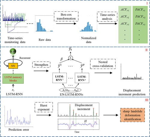
In this research, a deep-learning based data-driven framework is developed for predicting and monitoring deformed landslide displacements. The architecture of the proposed framework consists of three phases. A schematic diagram is presented in Figure 1. In Phase I, the time-series monthly precipitation, reservoir water level, and displacement data are normalized through Box–Cox transformation. Meanwhile, the ACFs and PACFs are computed to investigate the temporal dependencies of the time-series. In Phase II, the prediction models are constructed using EN-LSTM-RNNs to predict future incoming displacement. Month forward-chaining nested cross-validation is applied for training and validating the EN-LSTM-RNNs for each case study. To validate the effectiveness of the LSTM-RNN algorithm, five benchmarking machine learning algorithms are selected for performance comparison. In Phase III, the HEs are computed to monitor the sharp landslide deformation based on the prediction error produced by EN-LSTM-RNNs in the temporal domain. The prediction errors with respect to the incremental displacements are utilized to obtain the HE. Abnormal HEs are applied to monitor and detect sharp landslide deformation.

Figure 1. Architecture of the proposed data-driven framework.

2.1. Box–Cox transformation

The time-series landslide instant displacement and other triggering factors are time-dependent, non-stationary, and highly nonlinear. Outliers and the algorithm’s high non-linearity deteriorate the algorithm’s modelling performance. In this research, the Box–Cox transformation (Box and Cox 1964) is utilized to normalize the dataset and improve the prediction performance.

The Box–Cox transformation is a parametric power transformation technique that improves the additivity, normality, and homoscedasticity of the dataset (Box and Cox 1964). The Box–Cox transformation can be expressed by (1): (1) $$y\left(\lambda \right)=\{\begin{array}{c}\frac{y^{\lambda }-1}{\lambda },\lambda \ne 0\\ \mathrm{logy},\lambda =0\end{array}$$(1) where y represents the monitored instant displacement and λ denotes the transformation parameter to be identified. In accordance with previous research (Legendre and Borcard 2018), the maximum likelihood method is applied to estimate the power parameter λ. The log-likelihood function for λ can be expressed by (2): (2) $$L\left(\mathrm{\lambda }\right)=C-\frac{n}{2}\log \left({\widehat{\sigma }}^2\left(\lambda \right)\right)+(\lambda -1)\sum _{i=1}^n\log \left(y_i\right)$$(2) where n denotes the total number of displacement observations, $C=-\frac{n}{2}\ln 2\mathrm{\pi }-\frac{n}{2},$ and ${\widehat{\sigma }}^2$ represents the sample variance. λ can be determined by taking the partial derivatives of (2) to obtain the maximum likelihood estimation.

2.2. Autocorrelation analysis

Landslide instant displacement and its triggering factors including precipitation and reservoir water level have exhibited strong auto-correlation and seasonality patterns. Autocorrelation analysis can assist the discovery of temporal patterns and the construction of time-series model. Identifying these patterns through time-series in the temporal domain is essential for determining the optimal input and output scale to ensure the quality of the prediction outcome.

In this research, the autocorrelation analysis includes the computation of the ACF and PACF. The ACF (see (3)) represents the correlation coefficient between the current observation and its lag-k observation. The PACF (see (4)) represents the added contribution from the lag-k observation to the current observation as follows: (3) $${\rho }_k=\frac{\mathit{Cov}(x_t,x_{t-k})}{\sqrt{\mathit{V}\mathit{ar}\left(x_t\right)\mathit{Var}\left(x_{t-k}\right)}}=\frac{\mathit{Cov}(x_t,x_{t-k})}{\mathit{Var}\left(x_t\right)}=\frac{{\gamma }_k}{{\gamma }_0}$$(3) (4) $${\mathrm{\varnothing }}_k=\mathit{Corr}\left(x_t,x_{t-k}\right|x_{t-1},x_{t-2},\dots ,x_{t-k+1})$$(4) where x_t denotes the current data, x_t-k represents the lag-k historic observation, γ_k is the covariance between x_t and x_t-k, and γ₀ is the variance of the current observation. In practice, both the ACF and PACF are non-zero for most of the case studies in time-series types of problems. Intuitively, the ACF measures the correlation between the present value of the series and its past values. The PACF measures the hidden information (past residues) that may be correlated with the future present value after considering the effects of autocorrelation. Overall, based on the ACF and PACF, the contribution and correlation of the historic landslide instant displacement, precipitation, and water reservoir level to the current observation can be quantitatively assessed.

2.3. Long short-term memory recurrent neural network

The temporal data features play a crucial role in modelling and forecasting time-series displacement, precipitation, and water reservoir level. In this regard, a learning algorithm with the capacity to abstract the temporal data features from the previous data is the key to sufficient forecasting performance. The LSTM-RNN is a highly preferable candidate algorithm owing to its demonstrated capacity in learning temporal features.

The LSTM-RNN algorithm consists of two major components: the RNN and LSTM. The RNN is a sequence-based model that is fundamentally different from traditional feedforward neural networks, which can form the fundamental temporal correlations between the previous information and current circumstances. In time-series sector, this implies that the decision an RNN makes at time step t − 1 could impact the decision at any time step after t. The intrinsic structure of an RNN makes it highly preferable for time-series displacement modelling because the temporal correlation within displacement and its triggering factors are preserved well, which is crucial as discussed in previous studies (Li et al. 2018).

In practice, the RNNs are trained using backpropagation. However, learning long-range dependencies with RNNs is challenging owing to the gradient vanishing or exploding (Sutskever et al. 2014). Gradient vanishing refers to the exponential decrease of the fast norm of the gradient for long-term components to zero. It limits the RNN’s capacity to extract long-term temporal correlations. Meanwhile, the gradient explosion refers to the converse scenario, which also impacts the temporal feature extraction similarly (Turaga et al. 2008). To overcome this issue, the LSTM architecture has been introduced. It has become highly popular in many time-series applications (Mohammadi et al. 2018).

As described in (Irie et al. 2018), the LSTM-RNN includes a memory cell, an input gate, an output gate, and an additional forget gate in each building block. Let {x₁, x₂,…, x_t} denote a typical time-series sequence as LSTM’s input; here, x_t represents a multi-dimensional vector for real values. The LSTM-RNN can be expressed as (5)–(9): (5) $$i_t=\sigma (W_{xi}{x}_t+W_{hi}{h}_{t-1}+W_{ci}{c}_{t-1}+b_i)$$(5) (6) $$f_t=\sigma (W_{xf}{x}_t+W_{hf}{h}_{t-1}+W_{cf}{c}_{t-1}+b_f)$$(6) (7) $$c_t=f_t{c}_{t-1}+i_t\tanh (W_{xc}{x}_t+W_{hc}{h}_{t-1}+b_c)$$(7) (8) $$o_t=\sigma (W_{xo}{x}_t+W_{ho}{h}_{t-1}+W_{co}{c}_{t-1}+b_o)$$(8) (9) $${\overline{y}}_t=o_t\tanh \left(c_t\right)$$(9) where W_xi, W_hi, W_ci, W_xf, W_hf, W_cf, W_xc, W_hc, W_xo, W_ho and W_co are weight matrices for the corresponding inputs of the network activation functions; i_t, f_t, c_t and o_t denote the input gate, forget gate, memory cell state, and the output gate, respectively; $\overline{y_t}$ denotes the intermediate output vector; σ presents the sigmoid activation function; and tanh() represents the tanh function. The hyperparameters of LSTM-RNN need to be specified using cross-validation, which is described in the next subsection.

2.4. Ensemble learning using elastic net

In the field of machine learning, a single regressor (e.g., LSTM-RNN) is likely to converge to the optimal solution based on the specific data patterns contained in the training dataset. However, in certain scenarios, these identified patterns exist only in a certain portion of the training dataset and cannot be generalized to the whole dataset. Hence, ensemble learning can be utilized to enhance the performance over a group of regressors (see Figure 2).

Figure 2. Scheme of EN ensemble-based LSTM-RNN.

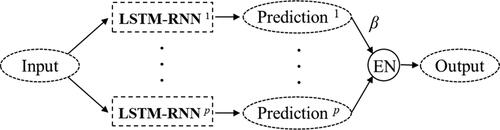
The EN ensemble regressor is a modified bagging technique that generates an ensemble of regressors. Proposed by Zou and Hastie (2005), the EN is a new regularization and variable selection method that considers strongly correlated features as a group. The EN algorithm contains both L1 and L2 regularization parameters and hence incorporates the benefits of both least absolute shrinkage and selection operator (LASSO) and ridge; both are conventional and widely utilized ensemble approaches. The objective function of EN is defined in (10): (10) $$\widehat{\beta }=\underset{\beta }{\mathrm{argmin}}{\Vert Y-X\beta \Vert }_2^2+{\lambda }_1{\Vert \beta \Vert }_1+{\lambda }_2{\Vert \beta \Vert }_2^2$$(10) where Y is the ground truth of the output, X is the vector containing all the prediction results from all the regressors, β denotes the correlation coefficient estimated with respect to all the regressors, and λ₁ and λ₂ are regularization coefficients for the L1-norm (i.e., LASSO) and L2-norm (i.e., ridge regression) penalties, respectively. The optimal values of λ₁ and λ₂ are determined by nested cross-validation, which is introduced in the next subsection.

In this study, we have produced five single LSTM-RNNs as our single regressors within the framework. The historic incremental displacement, predicted precipitation, and predicted water reservoir levels are all utilized as inputs in for each LSTM-RNN algorithm. The output is the instant displacement for the following month. An EN containing both the L1-norm and L2-norm serves as a regressor that aggregate the prediction outcomes from the LSTM-RNNs to derive the final prediction outcome. The regression coefficients as well as the two penalization parameters are tuned via nested cross-validation, respectively.

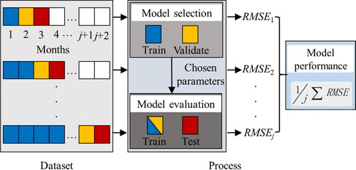
2.5. Month forward-chaining nested cross-validation

Traditional cross-validation (e.g., k-fold cross-validation) has become the benchmarking approach for validating machine learning/deep learning algorithms. However, in a time-series domain, traditional k-fold cross-validation should not be arbitrarily utilized owing to the temporal dependencies (e.g., auto-correlation or seasonality). With time-series data, particular care must be taken while splitting the data in the cross-validation procedures.

In this research, a month forward-chaining (Tashman 2000) is applied to cross-validate the time-series displacement, precipitation, and water reservoir level. In this method, each month is considered as the test set, and all previous data are assigned as training and validation dataset, as illustrated in Figure 3. Hence, all the temporal dependencies among the data points have been preserved. This method produces many training/testing data splits, and the error measurement in each split is averaged to compute a robust estimate of the model performance.

Figure 3. Month forward-chaining nested cross-validation.

2.6. State-of-art machine learning algorithms

In this research, four state-of-the-art machine algorithms (BPNN, ELM, SVM and classical LSTM-RNN) have been selected and compared with the proposed EN-LSTM-RNNs to validate the accuracy and effectiveness of our framework.

The BPNN model applied in this research is a commonly used neural network involving processing neurons organized into multiple layers (Moghaddam et al. 2016). It applies back-propagation (BP) to optimize the weights and biases in the hidden layers and hidden neurons to extract models based on the input data and the corresponding outputs. The sigmoid function is selected as the activation function in this study. The optimal number of hidden neurons and hidden layers are obtained through 10-fold cross-validation through the strategies presented in Table 1.

Table 1. Parameters selected for training via cross-validation.

Algorithm	Parameter	Details
BPNN	Hidden neuron	M = 10, 20, 30, 40, 50
	Hidden layers	N = 1, 2, 3, 4, 5
ELM	Hidden neuron	h = 2,4,6,8,…,98,100
SVM	Compacity factor	C = 1, 10, 100, 1000
	Gamma	γ = 0.001, 0.01, 0.1, 1
LSTM-RNN	Dropout	Dp = 0.2,0.3,0.4,0.5
	Epochs	Epochs = 30,40,50,60
EN	log(λ1)	log(λ) = 0, −1, −2, …, −5
	log(λ2)	log(λ) = 0, −1, −2, …, −5

The ELM algorithm is a single hidden-layer feedforward neural network (Huang et al. 2006). It is considered as a novel computing paradigm that enables a neural network to learn features with fast training speed and good generalization performance (Jiang et al. 2021). In this paper, the optimal number of hidden neurons is determined through 10-fold cross-validation by following the training strategies presented in Table 1.

The SVM model is a supervised learning method based on kernel functions used for classification, regression, and function approximation (Gunn 1998). Specific kernel functions are utilized to transform the original parameter space into a high-dimensional space, where a maximum margin hyper-plane is constructed. In this study, the radial basis function (RBF) is selected as the kernel function expressed in (11): (11) $$K(X,X\prime )=\hspace{0.17em}\text{exp}\hspace{0.17em}\left(\frac{-\Vert X-X\prime \Vert }{2{\sigma }^2}\right)$$(11) where X is the vector of the input data. The optimal parameter settings of the capacity factor C and the parameter γ = 1∕2σ² are evaluated through 10-fold cross-validation by following the strategies presented in Table 1.

In addition, for the proposed EN-LSTM-RNNs and classical LSTM-RNN, different parameters including dropout ratio and training epochs have been tested, as presented in Table 1.

2.7. Model evaluation metrics

To assess the performance of the proposed deep-learning framework in landslide displacement prediction, four metrics (namely, mean absolute error (MAE (12)), mean absolute percentage error (MAPE (13)), root mean square error (RMSE (14)), and hit rate (HR (15))) are selected in this study to evaluate the performances of all the machine learning algorithms tested. (12) $$\mathit{MAE}=\frac{1}{n}{\sum }_{t=1}^n\left|{\overline{y}}_t-y_t\right|$$(12) (13) $$\mathit{MAPE}=\frac{1}{n}{\sum }_{t=1}^n\left|\frac{{\overline{y}}_t-y_t}{y_t}\right|$$(13) (14) $$\mathit{RMSE}=\sqrt{\frac{1}{n}\sum _{t=1}^n{({\overline{y}}_t-y_t)}^2}$$(14) (15) $$HR=\frac{1}{N}\sum _{t=1}^{N}I\left(t\right)$$(15) where y_t denotes the actual data by field investigation, $\overline{y_t}$ represents the predicted outcome; and I() in (15) denotes the indication function expressed in (16): (16) $$I\left(t\right)=\{\begin{array}{c}1,if\left|\frac{{\overline{y}}_t-y_t}{y_t}\right|\le 0.1\\ 0,if\left|\frac{{\overline{y}}_t-y_t}{y_t}\right|>0.1\end{array}$$(16)

2.8. Hurst exponent

The HE, proposed by Hurst (1956, 1957) for use in fractal analysis, has been applied in various research domains, particularly in the finance community (Couillard and Davison 2005). It provides a measure for the long-term memory and factuality of a time-series data. Owing to its robustness with few assumptions required for any underlying system, it has broad applicability for time-series analysis in all domains. The HE ranges from zero to one. Based on the HE value (H), all time-series can be classified into the following three categories: (1) H = 0.5 indicates a random time-series (white noise), (2) 0 < H < 0.5 indicates an anti-persistent series, and (3) 0.5 < H < 1 indicates a persistent series. The random time-series is a Gaussian process with mean zero and a static standard deviation. The anti-persistent time-series contains the characteristic of mean-reversion, i.e., the values tend to revert to their mean. The persistent time-series indicates the presence of a significant trend wherein the values depart from the mean of the original series.

The HE can be computed by rescaled range analysis (R/S analysis). For a time-series, the R/S analysis can be performed as follows.

Step 1: Calculate the mean value m using (17): (17) $$m=\frac{1}{n}\sum _{t=1}^n{e}_t$$(17) where e_t is the prediction error of EN-LSTM-RNN.

Step 2: Calculate the mean adjusted time-series ae using (18): (18) $${ae}_t=e_t-m,\mathrm{}t=1,2,\dots ,n$$(18)

Step 3: Calculate the cumulative deviate time-series Z using (19): (19) $$Z_t=\sum _{i=1}^t{ae}_t,t=1,2,\dots ,n$$(19)

Step 4: Calculate the range of the time-series R using (20): (20) $$R_t=\max \left(Z_1,Z_2,\dots ,Z_t\right)-\min \left(Z_1,Z_2,\dots ,Z_t\right),t=1,2,\dots ,n$$(20)

Step 5: Calculate the standard deviation series S using (21): (21) $$S_t=\sqrt{\frac{1}{t}\sum _1^t{(e_t-u)}^2},t=1,2,\dots ,n$$(21) where u denotes the mean from e₁ to e_t.

Step 6: Calculate the rescaled range series (R/S) using (22): (22) $${\left(\raisebox{1ex}{$R$}\!\left/ \!\raisebox{-1ex}{$S$}\right.\right)}_t=\raisebox{1ex}{$R_t$}\!\left/ \!\raisebox{-1ex}{$S_t$}\right.,t=1,2,\dots ,n$$(22)

Step 7: H can be computed based on the fact that (R/S) increases with time following a power-law, as expressed in (23): (23) $${\left(\raisebox{1ex}{$R$}\!\left/ \!\raisebox{-1ex}{$S$}\right.\right)}_t={cv}^{\mathrm{*}}{t}^H$$(23) where cv is a constant. In this research, it is challenging to detect the sharp deformation and is hence a persistent time-series. Hence, the HE can be applied as an indicator to predict the incoming occurrences.

3. Field investigation and data collection

To evaluate the effectiveness of the proposed deep-learning framework, on-site displacement data collected from three landslide locations in Three Gorges Reservoir in China has been processed and investigated as case studies. As illustrated in Figure 4(a), the three selected landslides are Baishuihe, Muyubao and Shuping. They all located on the riverside of Yangtze River. All the three landslides are water-induced and have been widely discussed in literature. The summary of each landslide is presented in Table 2. The field investigation for each landslide is discussed in detail in the following subsections.

Figure 4. Overview of the study area. (a) Location of the Three Gorges Reservoir; (b) location of the three cases; (c) a top view of the Muyubao landslide; (d) aerial image of Baishuihe landslide; (e) aerial image of Shuping landslide.

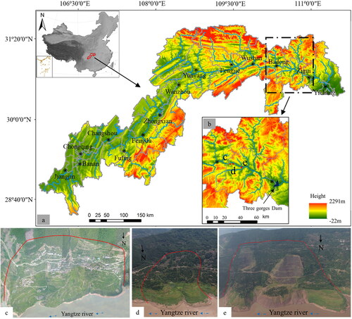
Table 2. Summary of the geological conditions in the case studies.

Landslide	Baishuihe	Muyubao	Shuping
Elevation (m.a.s.l)	75–390	120–425	60–470
Range (km^2)	0.42	1.80	0.55
Volume (m^3)	1260 × 10^4	9000 × 10^4	2750 × 10^4
Mean surface gradient (°)	30	15	50
Mean sliding zone thickness (m)	30	22	50
Bedrock geology	Coalseams, sandstones and mudstones	Carbonaceous siltstones and quartz sandstones	Sandstones, mudstones and limestones
Triggering factors	Precipitation and reservoir water level fluctuations	Precipitation and reservoir water level fluctuations	Precipitation and reservoir water level fluctuations

Note: m.a.s.l. represents the meter above the sea level as the elevation measurement unit.

3.1. Muyubao landslide

The Muyubao landslide is also located in Zihui county, China and is on the south river bank of Yangtze River. The total range of the landslide region is approximately 1.80 km². The total volume is 9000 × 10⁴ m³. The elevation of the landslide body ranges from 120 to 425 m.a.s.l. The average surface gradient is 15°, and the average slide body thickness is 22 m. The bedrock geology is composed of carbonaceous siltstones and quartz sandstones. The major triggering factors include precipitation and reservoir water level fluctuations. The conditions of Muyubao landslide is illustrated in Figure 4(c).

3.2. Baishuihe landslide

The Baishuihe landslide is located on the south bank of the Yangtze River in Zihui county and is approximately 60 km west of the Three Gorges Dam. This elevation of the fan-shaped landslide extends from 75 to 390 m.a.s.l. and covers an area of 0.42 km². The estimated volume of the slide is 1260 × 10⁴ m³. Moreover, it exhibits superficial cracking or distinct ground displacements. Its mean surface gradient is 30°, and the sliding zone thickness is 30 m. Its bedrock geology consists mainly of coal seams, sandstones, and mudstones.

The Baishuihe landslide should be conceived as an old landslide with frequent bedding slope failure in history, as illustrated in Figure 4(d). Most of the slope deformations in the past were triggered by precipitation and fluctuations of the water reservoir level. In August 2014, a landslide occurred with significant deformation and caused the evacuation of 85 individuals from 21 houses in local communities. Large farmlands and citrus orchards are still present on the slope. Hence, considering its morphological and geological conditions, public safety and land utilities are still at risk.

3.3. Shuping landslide

The Shuping landslide located in the Zigui county is another water-induced landslide. It is also in the river bank of Yangtze River near the town of Shazhenxi. The Shuping landslide has an elevation ranging from 60 to 470 m, covers a total area of 0.55 km², and has a total estimated volume of 2750 × 10⁴ m³. Its bedrock is composed of sandstones, mudstones, and limestones.

The Shuping landslide consists of two major blocks, as illustrated in Figure 4(e). The deformations on both the blocks are water-induced, and the intense conditions started in February 2004. Considering its risky geological condition, a total of 580 local inhabitants living in 163 houses have been instructed to evacuate since May 2004.

4. Experimental results

In this paper, the performance of the proposed deep-learning framework has been evaluated using the displacement data collected from three landslides in the Three Gorges Reservoir. The data for the three case studies are obtained via the GPS monitoring points in each landslide at monthly resolution (see Figure 5). Several reactivations are recorded during the monitoring period in each case study. Prior to the numerical analysis, all the monitoring data are subjected to pre-processing, including outlier removal and missing value imputation.

Figure 5. Historical landslide displacement, precipitation, and reservoir water level. (a) Muyubao landslide. (b) Baishuihe landslide. (c) Shuping landslide. (d) Reservoir water level.

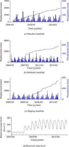
4.1. Data normalization and time-series analysis

After the data pre-processing, the Box–Cox normalization is employed in this research. The transformation power parameter λ expressed in (1) is approximated via cross-validation. Two normality evaluation metrics including Kolmogorov–Smirnov test (K–S test) (Razali and Wah 2011) and Cramer–von Mises test (C–vM test) (Evans et al. 2008) are conducted to evaluate the normality of the transformed displacement, precipitation, and reservoir water level. The normality tests results are summarized in Table 3.

Table 3. Normality test of Box–Cox transformed data.

Landslide	K-S test (p-value)			CvM test (p-value)
	Displacement	Precipitation	Reservoir water level	Displacement	Precipitation	Reservoir water level
Muyubao	0.45	0.21	0.26	0.26	0.17	0.33
Baishuihe	0.35	0.24		0.19	0.22
Shuping	0.27	0.19		0.12	0.15

As summarized in Table 3, all the normality test results have non-significant p values (p > 0.05) with respect to the transformed displacement, precipitation, and reservoir water level. This indicates that the dataset has approximately followed a Gaussian distribution.

The ACF and PACF with respect to the displacement, precipitation, and reservoir water level are also computed in this study. The ACF, which represents the linear dependence between the present and past lagged data, is expressed in (3). The PACF, which measures the autocorrelation between the present and past lagged data after removing the linear dependence, is expressed in (4). In this study, we applied the Ljung–Box test (Lee 2016) to measure the statistical significance of the computed ACFs and PACFs. The level of significance with regard to the lags of ACFs and PACFs is set as 0.05. The computational results are summarized in Table 4.

Table 4. Significant non-zero lags of ACF and PACF.

Landslide	ACF
	Displacement	Precipitation	Reservoir water level
Muyubao	1, 12, 13	1, 2, 4–8, 10–13	1–12
Baishuihe	1, 12	1–2, 4–8, 10–14
Shuping	1, 12, 13	1–2, 4–8, 10–14
	PACF
Landslide	Displacement	Precipitation	Reservoir water level
Muyubao	1, 12	1, 4–6, 12	1, 3, 8–10, 12
Baishuihe	1, 2, 12	1, 4–7, 12
Shuping	1, 12	1, 4–7

Note: All lags of ACF and PACF listed in this table are according to their p-value from Ljung–Box test.

According to Table 4, the precipitation and water reservoir levels reflected strong seasonal patterns. The first-three-month lag as well as the past-12-month lag exhibit significant non-zero autocorrelation, which indicates strong patterns of seasonality in the temporal domain. Meanwhile, the ACFs for the displacement in the three landslide case studies exhibit an exponential decay pattern. However, only the most recent lags for PACFs are significantly non-zero. Hence, it illustrates that the displacement only has autocorrelations without strong seasonality patterns.

4.2. Month forward-chaining cross-validation

In this experiment, the three landslide cases studies (namely, Muyubao, Baishuihe and Shuping) are investigated to construct the displacement prediction model. The proposed algorithm is compared with the four state-of-the-art machine learning algorithms described in Section 2.5. The data utilized in this experiment has been collected from GPS monitoring points in each landslide case study. The whole dataset has been split into training and testing datasets according to the 70% and 30% rule. The details of the dataset for each case study are summarized in Table 5.

Table 5. Experimental training and testing dataset.

Landslide	Training (nested cross-validation)		Testing
	Period	Number of samples	Period	Number of samples
Muyubao	Oct 2006–Oct 2012	73	Nov 2012–Jun 2015	32
Baishuihe	Jul 2003–Dec 2012	114	Jan 2013–Sep 2016	45
Shuping	Jul 2003–Jan 2010	79	Feb 2010–Oct 2012	33

In this study, all the hyperparameters in the tested algorithms are tuned and validated via month forward-chaining nested cross-validation. Thereby, the temporal dependencies within the dataset have been preserved well. In each training-validation experiment, the historic one-month to one-year data has been utilized for training. Moreover, the next one-month data has been utilized for validation. The month forward-chaining nested cross-validation results are illustrated in Figure 6.

Figure 6. Month forward chaining nested cross validation of all algorithms tested. a, d, g, and j are the evaluation for Muyubao landslide; b, e, h, and k are the evaluation for Baishuihe landslide; c, f, i, and l are the evaluation for Shuping landslide.

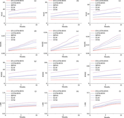
Figure 6 shows the experimental results of forward-chaining nested cross-validation for the different case studies. The cross-validation errors are evaluated by the four measurement metrics (namely, MAE, MAPE, RMSE and HR) discussed in Section 2.5. The computational results demonstrated that the proposed EN-LSTM-RNNs significantly outperform the other state-of-the-art machine learning algorithms tested; it produced the smallest prediction errors. All the hyperparameters of all the algorithms have been tuned to the optimal solution. The EN-LSTM-RNNs exhibited their outperformance in terms of prediction in the temporal domain, owing to the characteristics of its sequential learning structure and long-term memory. The testing outcome is presented in Table 6.

Table 6. Landslide displacement testing performance of all algorithms tested.

MAE (mm)
Landslide	EN-LSTM-RNN	LSTM-RNN	BPNN	ELM	SVM
Muyubao	14.96	18.55	32.21	34.91	44.13
Baishuihe	15.79	22.77	35.76	39.13	47.66
Shuping	18.36	28.57	47.07	49.25	65.58
MAPE
Landslide	EN-LSTM-RNN	LSTM-RNN	BPNN	ELM	SVM
Muyubao	1.43%	1.85%	3.11%	3.51%	3.89%
Baishuihe	0.96%	1.48%	2.41%	2.65%	3.50%
Shuping	1.32%	1.78%	3.46%	3.87%	4.42%
RMSE (mm)
Length	EN-LSTM-RNN	LSTM-RNN	BPNN	ELM	SVM
Muyubao	15.89	22.41	36.14	37.74	58.13
Baishuihe	17.99	27.49	42.76	44.61	69.17
Shuping	24.25	34.93	51.99	53.67	83.60
1-HR
Landslide	EN-LSTM-RNN	LSTM-RNN	BPNN	ELM	SVM
Muyubao	36.67%	38.91%	40.79%	46.14%	53.31%
Baishuihe	13.33%	14.08%	15.43%	17.47%	19.94%
Shuping	23.33%	25.49%	27.48%	29.81%	34.33%

According to Table 6, the proposed EN-LSTM-RNNs produces the lowest prediction error for all the three case studies presented. In Muyubao landslide, the MAPE values of the EN-LSTM-RNN, LSTM-RNN, BPNN, ELM, and SVM are 1.43%, 1.85%, 3.11%, 3.51% and 3.89%, respectively. In Baishuihe landslide, the RMSE of all five methods are 17.99, 27.49, 42.76, 44.61 and 69.17 successively using millimeter as the unit. The 1-HR in case Shuping are 23.33%, 25.49%, 27.48%, 29.81% and 34.33%. Therefore, it can be concluded that the proposed ensemble predicting framework outperforms when compared with the classical LSTM-RNN and other benchmarks. Meanwhile, the MAE values in all three cases of the proposed method are 14.96, 15.79, and 18.36, which are 20% less than the classical LSTM-RNN. Comparatively, for the case study of Baishuihe landslide, all MAPE values are lower compared with Muyubao and Shuping landslides which may be attributed to the intrinsic autoregressive and seasonal patterns that exist in its dataset. Meanwhile, according to the 1-HR values computed, over 85% of the predicted instance displacements fall into the 90% confidence interval of the actual displacement value in the case study of Baishuihe landslide, which is slightly higher than the case studies of Muyubao and Shuping landslides. The computational results imply that Baishuihe are more homogeneous with respect to the autoregressive and seasonal patterns in the temporal domain. In addition, it is noteworthy that the RMSEs are on an average higher than the measured MAE. This phenomenon indicates that the errors in the prediction of sharp landslide deformation (with large increment displacement) are statistical outliers and contribute more to the overall prediction errors measured. The identification of sharp landslide deformation based on the prediction error produced by EN-LSTM-RNNs is discussed in detail in the next subsection.

4.3. Measurement of long-term memory

As discussed in the literature (Li et al. 2018), the majority of the slide patterns in Three Gorges Reservoir belonged to two types of landslide motion: slower displacement and sharp landslide deformation. The long period of slower displacement results from semi-constant displacement rates over several months or most parts of the year. The sharp landslide deformation reflects steep positive gradients and exhibits ‘step-like’ patterns in the cumulative horizontal displacement plots (Massey et al. 2013). In the temporal domain, the increments in the slower displacement can be conceived as a persistent time-series exhibiting strong stationarity with limited temporal variation. Meanwhile, the sharp landslide deformation contains anti-persistent behaviour. This imparts complexity and uncertainty to the displacement modelling system.

In this research, the HE, which was designed to detect the persistence/anti-persistence in the time-series data, has been computed for detecting sharp landslide deformation. The prediction errors with respect to the incremental displacement produced by the EN-LSTM-RNNs algorithm are utilized in the computation. The computed HEs are based on window sizes ranging from 1 to 12 (similar to the training size for each month forward-chaining nested cross-validation experiment) and smoothed in the temporal domain. The experiments are conducted in accordance with the steps introduced in Section 2.8. The computational results of the three case studies are plotted in Figure 7.

Figure 7. Smoothed Hurst exponent corresponding to the incremental displacement in the temporal domain. (a) Muyubao landslide. (b) Baishuihe landslide. (c) Shuping landslide.

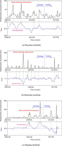
As shown in Figure 7, the smoothed HEs correspond to the incremental displacement in the temporal domain. As discussed in Section 4.2, the outliers (sharp landslide deformation) contribute more to the prediction errors. Hence, the anti-persistence (HE > 0.5 or HE < 0.5) detected from the prediction errors corresponds to the majority of the extremely sharp landslide deformation with large slide volumes. In contrast, the prediction errors are relatively small under a slower displacement. The prediction errors reflected persistent behaviour in the temporal domain, and the corresponding HEs are approximated to 0.5. Hence, the HEs can be utilized as an effective sensor to detect the hazardous sharp landslide deformation in the future.

5. Discussion

The historic precipitation and reservoir water level are highly correlated with the instant displacement values. Meanwhile, strong auto-correlation and seasonality patterns exist in the time-series precipitation and reservoir water level. Hence, an LSTM-RNN algorithm that can incorporate these complex patterns would exhibit sufficient performance in the prediction of landslide displacement.

Sharp landslide deformation and slower displacement composed the majority of the displacement patterns in all the water-induced landslides in Three Gorges Reservoir. The slower displacement accounts for over 80% of the displacement behaviours in the temporal domain and can be conceived as a persistent time-series. Nevertheless, the sharp landslide deformation is more hazardous to the local community owing to its intensified movement within a short period of time and its mass slide volume. In the temporal domain, the sharp landslide deformation illustrates an anti-persistent pattern in the displacement time-series. Therefore, in this study, we proposed the use of HE, which detects anti-persistence in time-series data to identify sharp landslide deformation.

The computational results are derived which can be attributed to the following three reasons: First, the dataset utilized in this study are very homogeneous and all case studies are from one macro region which all landslides are induced by water. There exists a strong dependency between the instant displacement and the water-related features according to the previous studies (Li et al. 2020b; Lian et al. 2018; Tao et al. 2020; Wang et al. 2019; Zhu et al. 2020). Hence, for other types of landslides or other time-series dataset, the accuracy and effectiveness still await further validation. Second, the triggering factors as precipitation and water reservoir levels have strong seasonal patterns and are also autoregressive. These temporal patterns are easy to be captured by the EN-LSTM algorithm which is designed to effectively capture the temporal features. For other non-water induced landslide, the triggering factors may not have such explicit temporal pattern which may increase the difficulty for training an accuracy regressors for predicting future landslide displacement. Third, all sharp landslide deformation with large instant displacement values can be perceived as statistical outliers compared with the other displacement patterns. The Hurst exponent is designed to capture such outliers in the temporal domain and has been widely applied in financial engineering sectors such as high-frequency trading systems. For the similar time-series problems, the proposed framework could be a feasible solution as well.

The advantages of the proposed framework can be summarized as three points: First, it is a pioneering research that uses deep-learning in time-series landslide displacement research. The proposed algorithm outperforms the state-of-the-art approaches in all the case studies. Secondly, this research applies month forward-chaining nested cross-validation to train and validate the time-series dataset. All the temporal data features such as auto-correlation and seasonality are preserved well during the cross-validation, in comparison with traditional 10-fold cross validation. Thirdly, the HE, which represents the relative tendency of the predicted displacement, has served as an effective indicator of fast seasonal displacement. An early warning system can be constructed by analysing the computed HE in the temporal domain.

In the present stage, similar as related research, displacement modelling and prediction are conducted based on single GPS point in each landslide. Nevertheless, the landslide displacement even varies with respect to the different monitoring location in the landslide slope. Hence, it may produce biasness using single GPS point to estimate the overall landslide displacement behaviour. Future displacement research should be directed toward generalizing spatial–temporal models that include both spatial and temporal features of multiple GPS points. A prominent contribution can be expected in landslide deformation studies through this strategy.

In addition, the HE, which measures the persistence/anti-persistence, has been widely discussed in time-series research. Owing to its high dependencies on data rescaling in the temporal domain, outliers in the low-frequency dataset may straightforwardly result in false discovery of anti-persistence in the temporal domain. In future research, the displacement and the triggering factors collected under high-frequency is likely to further improve the detection reliability of sharp landslide deformation.

6. Conclusions

In this study, a deep-learning framework for predicting and monitoring landslide deformation displacement was developed. In the data pre-processing step, the dataset was normalized and the outliers are removed. The proposed EN-LSTM-RNNs was constructed to predict the displacement and the month forward-chaining nested cross-validation was utilized as the training strategy. Comparative analysis is performed against four state-of-the-art machine learning algorithms. Then, the HE is used to measure the future prediction for identifying sharp landslide deformation. To validate the robustness of the proposed framework, three landslides in Three Gorges Reservoir, China have been selected as case studies.

The experimental results of the three case studies have demonstrated that the displacement, precipitation, and reservoir water level exhibit strong seasonality and auto-correlation patterns in the temporal domain. Moreover, the proposed EN-LSTM-RNNs outperforms the other state-of-the-art machine learning algorithms tested here, for modelling landslide displacement. In addition, the computed time-dependent HE has been demonstrated to be indicative of incoming fast seasonal displacements.

In practice, this proposed framework enables us to predict and monitor landslide displacement in real-time. The time-dependent HE can function as the indicator for predicting incoming fast seasonal displacement for sharp slope deformation. In the future, the transformer which contains the self-attention method could be utilized to further improve the performance of deformation prediction tasks.

Data available statement

Some or all data, models, or code that support the findings of this study are available from the corresponding author upon reasonable request.

Disclosure statement

No potential conflict of interest was reported by the authors.

Additional information

Funding

This research was supported by the Science Fund for Innovative Research Groups of the National Natural Science Foundation of China (Grant No. 41521002), the Major projects of the National Natural Science Foundation of China (Grant No. 41790445), the Opening fund of State Key Laboratory of Geohazard Prevention and Geoenvironment Protection (Chengdu University of Technology) (Grant No. SKLGP2021K014), “Miaozi project” of scientific and technological innovation in Sichuan Province, China (Grant No. 2021090), and the Project of remote sensing identification and monitoring of geological hazards in Sichuan province, CN (2020) (Grant No. 510201202076888).

References

- Box GEP, Cox DR. 1964. An analysis of transformations. J R Stat Soc: Ser B. 26(2):211–252.
- Chousianitis K, Del Gaudio V, Kalogeras I, Ganas A. 2014. Predictive model of Arias intensity and Newmark displacement for regional scale evaluation of earthquake-induced landslide hazard in Greece. Soil Dyn Earthquake Eng. 65:11–29.
- Couillard M, Davison M. 2005. A comment on measuring the Hurst exponent of financial time series. Physica A. 348:404–418.
- Dietrich WE, Reiss R, Hsu ML, Montgomery DR. 1995. A process‐based model for colluvial soil depth and shallow landsliding using digital elevation data. Hydrol Process. 9(3-4):383–400.
- Efstratiadis A, Nalbantis I, Koutsoyiannis D. 2015. Hydrological modelling of temporally-varying catchments: facets of change and the value of information. Hydrol Sci J. 60(7-8):1438–1461.
- Evans DL, Drew JH, Leemis L. 2008. M., The distribution of the Kolmogorov–Smirnov, Cramer–von Mises, and Anderson–Darling test statistics for exponential populations with estimated parameters. Commun Stat-Simulat Comput. 37(7):1396–1421.
- Falk T, Mai D, Bensch R, Çiçek Ö, Abdulkadir A, Marrakchi Y, Böhm A, Deubner J, Jäckel Z, Seiwald K, et al. 2019. A., U-Net: deep learning for cell counting, detection, and morphometry. Nat Methods. 16(1):67–70.
- Gao G, Meguid MA. 2018. On the role of sphericity of falling rock clusters—insights from experimental and numerical investigations. Landslides. 15(2):219–232.
- Ghorbanzadeh O, Blaschke T, Gholamnia K, Meena S, Tiede D, Aryal J. 2019. Evaluation of different machine learning methods and deep-learning convolutional neural networks for landslide detection. Remote Sens. 11(2):196..
- Greenspan H, Van Ginneken B, Summers RM. 2016. Guest editorial deep learning in medical imaging: Overview and future promise of an exciting new technique. IEEE Trans Med Imaging. 35(5):1153–1159.
- Gudiyangada Nachappa T, Kienberger S, Meena SR, Hölbling D, Blaschke T. 2020. Comparison and validation of per-pixel and object-based approaches for landslide susceptibility mapping. Geomat Nat Hazards Risk. 11(1):572–600.
- Gunn SR. 1998. Support vector machines for classification and regression. ISIS Technic Rep. 14:5–16. http://see.xidian.edu.cn/faculty/chzheng/bishe/indexfiles/new_folder/svm.pdf.
- He Y, Fei F, Wang W. 2018. Predicting manufactured shapes of a projection micro-stereolithography process via convolutional encoder-decoder networks. Paper presented at: ASME 2018 International Design Engineering Technical Conferences and Computers and Information in Engineering Conference. American Society of Mechanical Engineers: V01BT02A033-V01BT02A033.
- Huang GB, Zhu QY, Siew CK. 2006. Extreme learning machine: theory and applications. Neurocomputing. 70(1–3):489–501.
- Hurst HE. 1956. Methods of using long-term storage in reservoirs. Proc Inst Civ Eng. 5(5):519–543.
- Hurst HE. 1957. A suggested statistical model of some time series which occur in nature. Nature. 180(4584):494–494.
- Irie K, Lei Z, Schlüter R, Ney H. 2018. Prediction of LSTM-RNN full context states as a subtask for N-gram feedforward language models. Paper presented at 2018 IEEE International Conference on Acoustics, Speech and Signal Processing (ICASSP). IEEE. p. 6104–6108.
- Jiang Y, Xu Q, Lu Z, Luo H, Liao L, Dong X. 2021. Modelling and predicting landslide displacements and uncertainties by multiple machine-learning algorithms: application to Baishuihe landslide in Three Gorges Reservoir, China, Geomatics. Nat Hazards Risk. 12(1):741–762.
- Jibson RW. 2007. Regression models for estimating coseismic landslide displacement. Eng Geol. 91(2–4):209–218.
- Lee T. 2016. Wild bootstrap Ljung–Box test for cross correlations of multivariate time series. Econ Lett. 147:59–62.
- Legendre P, Borcard D. 2018. Box–Cox‐chord transformations for community composition data prior to beta diversity analysis. Ecography. 41(11):1820–1824.
- Lewis R, Reinsel GC. 1985. Prediction of multivariate time series by autoregressive model fitting. J Multivariate Anal. 16(3):393–411.
- Li H, Xu Q, He Y, Deng J. 2018. Prediction of landslide displacement with an ensemble-based extreme learning machine and copula models. Landslides. 15(10):2047–2059.
- Li H, Xu Q, He Y, Fan X, Li S. 2020b. Modeling and predicting reservoir landslide displacement with deep belief network and EWMA control charts: a case study in Three Gorges Reservoir. Landslides. 17(3):693–707.
- Li SH, Wu LZ, Chen JJ, Huang RQ. 2020a. Multiple data-driven approach for predicting landslide deformation. Landslides. 17(3):709–718.
- Lian C, Philip Chen CL, Zeng Z, Yao W, Tang H. 2016. Prediction intervals for landslide displacement based on switched neural networks. IEEE Trans Rel. 65(3):1483–1495. https://doi.org/http://dx.doi.org/10.1109/TR.2016.2570540.
- Lian C, Zhu L, Zeng Z, Su Y, Yao W, Tang H. 2018. Constructing prediction intervals for landslide displacement using bootstrapping random vector functional link networks selective ensemble with neural networks switched. Neurocomputing. 291:1–10.
- Lu P, Rosenbaum MS. 2003. Artificial neural networks and grey systems for the prediction of slope stability. Nat Hazards. 30(3):383–398.
- Ma L, Sun B, Li Z. 2017. Bagging likelihood-based belief decision trees. Paper presented at 2017 20th International Conference on Information Fusion (Fusion). IEEE. p. 1–6.
- Massey CI, Petley DN, McSaveney MJ. 2013. Patterns of movement in reactivated landslides. Eng Geol. 159:1–19.
- Meena S, Ghorbanzadeh O, Blaschke T. 2019. A comparative study of statistics-based landslide susceptibility models: a case study of the region affected by the Gorkha earthquake in Nepal. IJGI. 8(2):94..
- Meena SR, Ghorbanzadeh O, van Westen CJ, Nachappa TG, Blaschke T, Singh RP, Sarkar R. 2021. Rapid mapping of landslides in the Western Ghats (India) triggered by 2018 extreme monsoon rainfall using a deep learning approach. Landslides. 18(5):1937–1950.
- Meng Q, Wang H, He M, Gu J, Qi J, Yang L. 2020. Displacement prediction of water-induced landslides using a recurrent deep learning model. Eur J Environ Civil Eng. 1–15.
- Moghaddam AH, Moghaddam MH, Esfandyari M. 2016. Stock market index prediction using artificial neural network. J Econ, Fin Administrat Sci. 21(41):89–93.
- Mohammadi M, Al-Fuqaha A, Sorour S, Guizani M. 2018. Deep learning for IoT big data and streaming analytics: a survey. IEEE Commun Surv Tutorials. 20(4):2923–2960.
- Montgomery DR, Dietrich WE. 1994. A physically based model for the topographic control on shallow landsliding. Water Resour Res. 30(4):1153–1171.
- Ouyang T, He Y, Li H, Sun Z, Baek S. 2019. Modeling and forecasting short-term power load with copula model and deep belief network. IEEE Trans Emerg Top Comput Intell. 3(2):127–136.
- Pradhan B. 2013. A comparative study on the predictive ability of the decision tree, support vector machine and neuro-fuzzy models in landslide susceptibility mapping using GIS. Comput Geosci. 51:350–365.
- Razali NM, Wah YB. 2011. Power comparisons of shapiro-wilk, kolmogorov-smirnov, lilliefors and Anderson-Darling tests. J Stat Model Anal. 2:21–33.
- Saito M. 1965. Forecasting the time of occurrence of a slope failure. Paper presented at the Proceedings of the 6th international conference on soil mechanics and foundation engineering, Montre al, Que. Pergamon Press, Oxford. p. 537–541. https://ci.nii.ac.jp/naid/10003436025/.
- Shihabudheen KV, Pillai GN, Peethambaran B. 2017. Prediction of landslide displacement with controlling factors using extreme learning adaptive neuro-fuzzy inference system (ELANFIS). Appl Soft Comput. 61:892–904.
- Sutskever I, Vinyals O, Le QV. 2014. Sequence to sequence learning with neural networks. Adv Neural Inform Process Syst. 3104–3112. http://papers.nips.cc/paper/5346-sequence-to-sequence-learning-with-neural-networks.
- Tao ZG, Zhu C, He MC, Karakus M. 2021. A physical modeling-based study on the control mechanisms of Negative Poisson's ratio anchor cable on the stratified toppling deformation of anti-inclined slopes. Int J Rock Mech Min Sci. 138:104632..
- Tao ZG, Zhu C, He MC, Liu KM. 2020. Research on the safe mining depth of anti-dip bedding slope in Changshanhao Mine. Geomech Geophys Geo-Energy Geo-Resour. 36(6):1–20.
- Tashman LJ. 2000. Out-of-sample tests of forecasting accuracy: an analysis and review. Int J Forecast. 16(4):437–450.
- Tavakkoli S, Shahabi H, Jarihani B, Ghorbanzadeh O, Blaschke T, Gholamnia K, Meena S, Aryal J. 2019. Landslide detection using multi-scale image segmentation and different machine learning models in the higher Himalayas. Remote Sens. 11(21):2575..
- Tiwari AK, Albulescu CT, Yoon SM. 2017. A multifractal detrended fluctuation analysis of financial market efficiency: comparison using Dow Jones sector ETF indices. Physica A. 483:182–192.
- Turaga P, Chellappa R, Subrahmanian VS, Udrea O. 2008. Machine recognition of human activities: a survey. IEEE Trans Circuits Syst Video Technol. 18(11):1473–1488.
- Voight B. 1989. A relation to describe rate-dependent material failure. Science. 243(4888):200–203. https://science.sciencemag.org/content/243/4888/200.
- Wang Y, Tang H, Wen T, Ma J. 2019. A hybrid intelligent approach for constructing landslide displacement prediction intervals. Appl Soft Comput. 81:105506–105516.
- Xu Q, Li H, He Y, Liu F, Peng D. 2019. Comparison of data-driven models of loess landslide runout distance estimation. Bull Eng Geol Environ. 78(2):1281–1294.
- Xu W, Meng Q, Wang R, Zhang J. 2016. A study on the fractal characteristics of displacement time-series during the evolution of landslides. Geomat Nat Hazards & Risk. 7(5):1631–1644.
- Yang B, Yin K, Lacasse S, Liu Z. 2019. Time series analysis and long short-term memory neural network to predict landslide displacement. Landslides. 16(4):677–694.
- Yildirim O, Baloglu UB, Tan RS, Ciaccio EJ, Acharya UR. 2019. A new approach for arrhythmia classification using deep coded features and LSTM networks. Comput Methods Programs Biomed. 176:121–133.
- Zhu C, He MC, Karakus M, Cui XB, Tao ZG. 2020. Investigating toppling failure mechanism of anti-dip layered slope due to excavation by physical modelling. Rock Mech Rock Eng. 53(11):5029–5050.
- Zhu C, He MC, Karakus M, Zhang XH, Tao ZG. 2021. Numerical simulations of the failure process of anaclinal slope physical model and control mechanism of negative Poisson's ratio cable. Bull Eng Geol Environ. 80(4):3365–3380.
- Zou H, Hastie T. 2005. Regularization and variable selection via the elastic net. J Royal Stat Soc B. 67(2):301–320.