Effect of spatial resolution and data splitting on landslide susceptibility mapping using different machine learning algorithms

Abstract

With the increasing computational facilities and data availability, machine learning (ML) models are gaining wide attention in landslide modeling. This study evaluates the effect of spatial resolution and data splitting, using five different ML algorithms (naïve bayes (NB), K nearest neighbors (KNN), logistic regression (LR), random forest (RF) and support vector machines (SVM)). The maps were developed using twelve landslide conditioning factors at two different resolutions, 12.5 m and 30 m. To identify the effect of data splitting on model performance, 2162 landslide points and an equal number of non-landslide points were used for training and testing the models using k-fold cross-validation, by varying the number of folds from two to ten. Results indicated that the spatial resolution of the dataset affects the performance of all the algorithms considered, while the effect of data splitting is significant in KNN and RF algorithms. All the algorithms yielded better performance while using the dataset with 12.5 m resolution for the same number of folds. It was also observed that the accuracy and area-under-the-curve values of 7, 8, 9, and 10-fold cross-validations with 30 m resolution was better than 2 and 3-fold cross-validations using 12.5 m resolution, in the case of RF algorithm.

Keywords:

• Landslides
• machine learning
• GIS
• susceptibility
• Idukki

1. Introduction

Landslide is one of the most severe geohazards, and it has severe effects on human life in mountainous terrain across the world. The recent increase in extreme climate events, urban expansion and unplanned development due to rapid population growth have increased the risk due to landslides. The hilly areas are being used for urban expansions and infrastructural developments, which in turn expose more elements to the risk due to landslides. This scenario calls for the requirement of landslide hazard zonation, for identifying the highly susceptible landslide zones that can help in landslide risk reduction and in framing the future land development strategies. The term ‘landslide susceptibility’ denotes the possibility of a landslide happening in a location, subjected to some conditioning factors which includes the local hydro-meteor-geological conditions, which can help in estimating the locations where landslides are expected to occur (Reichenbach et al. 2018). Landslide susceptibility maps are useful in management of landslide hazards and decision making in vulnerable areas (van Westen et al. 2006; Akgun 2012). Landslide susceptibility mapping (LSM) is carried out by government and non-governmental agencies using different modelling approaches. The earlier methods were based on expert opinions, which got replaced by a variety of physical-based (Sorbino et al. 2010; Formetta et al. 2016), analytical (Yalcin 2008) and statistical-based models (Bai et al. 2008; Akgun and Türk 2010; Pradhan 2013; Piciullo et al. 2018). The first attempts date back to the 1970s, and since then, the methods used for LSM are being constantly updated with technological advancements. The data driven models based on machine learning (ML) have proven to outperform all the conventional approaches in LSM (Pham et al. 2016). The advancements in geographical information systems (GIS) and easy accessibility to geospatial data have played a crucial role in the evolution of LSM using data driven models. Different machine learning models are being used for LSM, since the mid-2000s. Different ML techniques are widely accepted solutions for spatial analytics of big data (Qiu et al. 2016; Zhou et al. 2017; Singh et al. 2018). They have outperformed other models, as the theoretical knowledge of the problem for wider extents and presumptions in statistical models is unknown (Lary et al. 2016; Dou et al. 2019). ML does not require a pre assumed model, as in the case of statistics, and the algorithm learns the association between the landslides and the different conditioning factors, using the provided data. The initial studies using ML were based on Logistic Regression (LR). LR is a statistical tool, used to solve binary classification problems, later adopted by ML. For better accuracy, advanced ML models like Naïve Bayes (NB), K Nearest Neighbors (KNN), Decision Trees (DT), Support Vector Machines (SVM) and Random Forest (RF) are being widely used in LSM for more than a decade. Recently, many ensemble algorithms are being used for the performance enhancement of ML models (Dou et al. 2020; Merghadi et al. 2020; Pham et al. 2020; Wang et al. 2020), but an ensemble model does not necessarily result in better performance. In this study, the focus is on the effect of spatial resolution and data splitting only, and Random Forest is the only ensemble algorithm discussed in this study.

The quality of the input data is a key factor in deciding the performance of any machine learning model (Lima et al. 2021). In this study, the effect of the spatial resolution and the ratio of training and testing data are explored in detail. Effect of spatial resolution has been performed by evaluating scale effects of topographic variables in landslide susceptibility models using different resolutions of digital elevation models (DEM). The DEM resolution is a key factor, as several other landslide conditioning factors, like slope and aspect, are derived from the DEM layer. A general observation is that fine resolution of DEM would result in better performance, but the previous studies do not agree with this statement (Pradhan and Sameen 2017). A study on Sydney basin in Australia with different DEM resolutions varying from 2 m to 40 m proved that the best performance was obtained for 10 m DEM, using decision trees, which used 80% data for training and 20% for testing (Palamakumbure et al. 2015). Pradhan and Sameen (2017) prepared susceptibility maps for Cameron Highlands, in Malaysia for DEM resolutions varying from 1 to 30 m. They have used the elevation data from two different sources, i.e., LiDAR sensor and ASTER sensor, and the comparison showed that the data collected from LiDAR generated better landslide susceptibility maps. The study was conducted using LR method, and the best results were obtained for a resolution of 2 m. In a study conducted at Baxie river basin in China (Chen et al. 2020), the spatial resolution of DEMs were varied from 30 m to 90 m and the best performance was obtained for DEM with 70 m resolution. Another study conducted for Arno river basin in Italy concludes that spatial resolution of 50 m to 100 m has yielded optimum results, using RF algorithm (Catani et al. 2013). The study was conducted by varying spatial resolution from 10 m to 500 m, and the resolution of 100 m was further used for regional scale LSM for other parts of Italy as well (Luti et al. 2020). This study used three different statistical approaches, the frequency ratio, weights-of-evidence and index of entropy and the training to test dataset ratio was 70:30. The effect of spatial resolution, data splitting and their effects on different machine learning approaches are still less explored in the previous studies. The recent literature shows a shift toward cross-validation techniques for LSM using machine learning, but the number of folds is chosen randomly (Merghadi et al. 2020). The value of ‘k’ or the number of folds determines the train: test ratio, which highly influences the performance of any ML model. There is no clear agreement about the best model for LSM, and hence the choice of model has to be determined specifically for each case, through quantitative comparison. In this study, the performance of different machine learning models (NB, LR, KNN, RF and SVM) are evaluated with respect to the DEM resolution and number of folds used for validation.

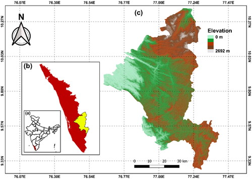
To check the effect of DEM resolution and data splitting in the performance of different ML algorithms used for LSM, a study area in the Western Ghats of India has been chosen. The location is Idukki district in the state of Kerala, which is highly affected by landslides. More than 2000 landslides were reported in the recent disaster that happened in 2018 August, and the severity is increasing every year (Abraham et al. 2019). The increasing number of landslides is creating havoc during the monsoon seasons. The landslide inventory data of 2018 shows a significant number of landslides have occurred outside the hazard zones, as depicted in the existing landslide susceptibility map for Idukki. Hence, the region direly needs an updated landslide susceptibility map, which can be used by the authorities as a tool for risk reduction.

2. Study area

India contributes 16% of the total rainfall induced landslides across the world (Froude and Petley 2018), and the Himalayas (Dikshit and Satyam 2018) and Western Ghats (Vishnu et al. 2019; Abraham et al. 2021; Meena et al. 2021) are two highly susceptible landslide zones in the country. The Western Ghats runs parallel to the western coast of the Indian peninsula, traversing from Gujarat in the North to Tamil Nadu in the south. The occurrence of rainfall induced landslides are increasing considerably and a notable increase is observed in the Western Ghats since 2018 (Abraham et al. 2021). The high intensity rainfalls have resulted in a notable increase in the number of landslides since 2018. Idukki is a hilly district belonging to the Western Ghats, spanning across an area of 4358 km². This ecologically sensitive zone has faced severe challenges from natural disasters, especially landslides during monsoon seasons. The unplanned infrastructural development and land use changes are exposing more elements to landslide risk, and it is high time that proper risk reduction strategies are to be developed for the region (Kanungo et al. 2020; Jones et al. 2021).

The district is drained by four major rivers and its tributaries, with a strong drainage network. Three of these rivers flow to the west and one towards east. The district also houses many hydro-electric projects and serves as the major power source for the state of Kerala. The topography of the district varies from north to south, resulting in varying climatic conditions across the district. The least rainfall in Idukki is recorded in the northern parts and the amount increases towards south (Abraham et al. 2021). More than 60% of the average annual rainfall is contributed by the north-east monsoon season, which triggers landslides in the district due to extreme rainfall events.

More than half of the area of Idukki belongs to forest and the rocks are composed of peninsular gneissic complex, migmatite complex and charnockite group from north to south (Department of Mining and Geology Kerala 2016). The rocks of the Peninsular gneissic complex are found in the northern part of the district. The granite gneiss rocks of Archean age are very hard and well foliated. The central area of the district is dominated by the migmatite complex, represented by biotite gneiss and hornblende biotite gneiss. Similar to the peninsular gneissic complex, migmatite complex is also very hard and foliated (Department of Mining and Geology Kerala 2016). A major portion of the district in the southern and south central part is composed of rocks of charnockite group, represented by pyroxene granulite, magnetite quartzite and charnockite (Geological Survey of India 2010). Among these, charnockite is spread across the area and the other two are found as linear bands, aligned parallel to the foliation trend. Minor fraction of Khondalite group, acidic intrusive and basic intrusive rocks are also found across the district, along with the other three major groups. The lower elevation region in the western part of the district (Figure 1) belongs to pediment complex, while the remaining area is formed by structural cum denudational hills, on Precambrian rock formations. The region consists of hills with thin cover of soil, laid over the basement rocks. The highly dissected hills and valleys of the district are prone to landslides and cause severe destruction. The forest cover of the region is composed of thick forest loam soil, formed by weathering of rock, rich in organic matter (Department of Mining and Geology Kerala 2016). The midlands of the district, with lesser elevation, are composed of lateritic soil with less organic content and high permeability. The valley regions of the district are composed of transported soil, with fine particle size, and the river banks are formed by highly fertile alluvial soil (Department of Mining and Geology Kerala 2016).

Figure 1. Locations of the study area: a) India; b) Kerala; and c) Idukki.

Agriculture and tourism are the major income sources of this district, and the transportation network requirements often lead to cutting of slopes without lateral support. The regions with elevation up to 1500 m are considered being plateau and most of the district belongs to this category. Most of the built-up area in the district falls in the midlands and the plateau region. The highest number of landslides in Idukki occurs along the major roads, unsettling the transport facilities. The hill stations and plantations, which are tourist hubs, often witness slope failures during monsoon seasons. The road and drainage network plays a substantial part in the triggering of landslides in this region, which has to be explored in detail. The increasing number of casualties due to landslides every year demands the necessity of proper planning for further development and land use changes. Hence, this study attempts to prepare data driven landslide susceptibility maps for Idukki, using different machine learning approaches and explores the effect of resolution and data splitting in the performance of different machine learning models.

3. Methodology

The study focuses on understanding the effect of spatial resolution and data splitting in LSM, using different ML algorithms. The procedure is represented schematically in Figure 2. The first step is the preparation of landslide inventory data. The landslides were represented using point data, at the crown of each landslide. The data is split into two parts, training and testing. The data splitting is carried out with different train: test ratios and k-fold validation were performed. The methodology depicted in Figure 2 has been repeated for different values of k, varying from 2 to 10.

Figure 2. Schematic diagram representing the methodology flow chart.

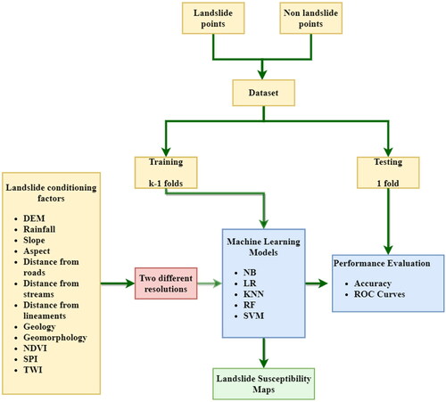
The landslide conditioning factors selected for the study are: elevation, aspect, slope, geology, rainfall, geomorphology, distance from roads, distance from streams, distance from lineaments, Topographic Wetness Index (TWI), Normalized Difference Vegetation Index (NDVI), and Stream Power Index (SPI). The definition of landslide conditioning factors is not straightforward and requires detailed knowledge of the geomorphological evolution of the study areas (Pradhan and Sameen 2017). Hence, the factors were selected considering the different aspects that may trigger landslide: – the elevation, slope, drainage characteristics, vegetation, geology, geomorphology and rainfall. These layers were collected from remote sensing data and published maps from different sources, rasterized and prepared the database using GIS software. The layers were then used to develop the landslide susceptibility maps using different machine learning models.

3.1. Data and preprocessing

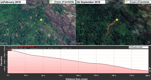
The quality of data is the key factor in determining the outputs of every data-driven model. Hence, data collection is a process to be carried out with utmost care and accuracy (Bui et al. 2012). The landslide inventory data has been prepared using Google earth imageries. The landslides were identified by comparing the images before and after August 2018 and the crown point was identified using the elevation profile of the terrain (Figure 3). The dataset has been prepared specifically for LSM, as the existing dataset available for the district (Abraham et al. 2021), is focused on the time of occurrence of landslides, using approximate landslide locations. The prepared dataset was found to be in good agreement with the database published by Hao et al. (2020). By this procedure, a total of 2162 landslide points were recognized in the administrative boundary of Idukki region. Out of the total landslides, 65.6% were classified as shallow landslides, 31.3% as debris flows and remaining 3.1% as rockslides. An equal number of points with no landslides were also created randomly inside the polygon, using the existing landslide susceptibility map for Idukki and the slope map of Idukki. The points were selected in flat terrains outside the existing susceptibility maps. These landslide and non-landslide points were used for training and testing each machine learning model used in this study.

Figure 3. Procedure of preparation of landslide inventory data: a) Google earth image before event; b) Google earth image after event; and c) elevation profile.

The DEM for the study area was derived from two different sources, the Alos Palsar DEM (ASF DAAC 2015) and the Cartosat DEM (National Remote Sensing Centre 2015). Alos Palsar DEM is a Radiometrically Terrain Corrected (RTC) product from the Alaska Satellite Facility (ASF DAAC 2015). The high resolution DEMs are available at 12.5 m $\times$ 12.5 m in the projected coordinate system. CartoDEM is developed using Augmented Stereo Strip Triangulation (ASST) by Indian Space Research Organisation. The resolution of DEM is 1 arc second (approximately 30 m) in the geographic coordinate system. In this manuscript, the Alos Palsar DEM is referred to as 12.5 m resolution DEM and CartoDEM as 30 m resolution DEM for convenience. The difference in data collected from the two sources and the different conditioning factors derived from DEM for 100 random points are plotted in Figure 4.

Figure 4. Comparison of different DEM derived layers using 12.5 m resolution and 30 m resolution: a) elevation, b) slope, c) aspect, d) TWI, and e) SPI.

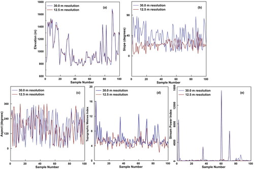
Slope, aspect, SPI and TWI layers were prepared from the DEM. The difference in altitude values of the two different DEMs will affect the values of these layers as well (Pradhan and Sameen 2017). As depicted in Figure 4, the variation in elevation values is negligible when both layers are compared. However, this minor variation has severe impacts on the DEM derived layers. Hence, the resolution of DEM is a critical factor in determining the quality of results and all these layers were developed using the DEMs of two different resolutions. Slope is a significant parameter in the process of LSM. It is the ratio of vertical distance to horizontal distance between two specified points, expressed using the tangent angle. The slope angle varies from 0 to 90 degrees and studies on LSM supports the consensus on the notion of considering slope as an important parameter in the initiation of landslides. The term aspect indicates the orientation of the slope face, expressed as an angle varying from 0 to 360 degrees, starting from north, in the clockwise direction, they are classified into 8 categories with a difference of 45 degrees each. The literature says that the slope aspect is critical when landslides are triggered after superficial cracks (tension cracks) are formed in clay (Capitani et al. 2013). These types of landslides are detected in the study area, and it is very common that long tension cracks can be identified at the crown of landslides much before the occurrence of landslides. Hence, aspect maps are also prepared using the DEM, for two different resolutions.

The drainage maps were developed for two different resolutions and were verified using google earth and minor corrections were made. The stream network was then used to calculate the distance from the stream layer of LSM. The flow accumulation maps were also developed using both the DEMs, for the calculation of SPI and TWI. SPI indicates the erosive power of flowing water, calculated using the slope and contributing area. SPI estimates positions where a flow path or gully is likely to form on the landscape. TWI is a wetness index, commonly used to quantify topographic control on hydrological processes. From the flow accumulation $(FA)$ map, SPI and TWI were calculated using the equations listed below, where $i\mathrm{ }$ is the index of each grid cell of the DEM: (1) $$\mathrm{SPI}={\mathrm{FA}}_{\mathrm{i}}\times \text{tan}\mathrm{ }\left({\mathrm{Slope}}_{\mathrm{i}}\right)$$(1) (2) $$\mathrm{TWI}=\ln \mathrm{ }\left(\frac{{\mathrm{FA}}_{\mathrm{i}}}{\text{tan}\mathrm{ }\left({\mathrm{Slope}}_{\mathrm{i}}\right)}\right)\mathrm{ }$$(2)

The rainfall data for the study area was collected from the Indian Meteorological Department (IMD) for four rain gauges in the study area. The average annual rainfall data collected from these points were estimated using Inverse Distance Weighted (IDW), which is a widely followed method of interpolation of rainfall data (Gilewski 2021; Jaya et al. 2021). In IDW, the cell values are determined using a linearly weighted combination of the sample points. The weight is inversely proportional to the remoteness from a point to the cell. The NDVI layer was prepared using Landsat 8 images, acquired on 21st January 2018. The NDVI values indicate the greenness of a location. Higher NDVI values indicate the presence of vegetation, while the least values are observed in water bodies. NDVI is computed as the ratio between the red (R) and near infrared (NIR) values, and can be calculated from Landsat 8 images using the following equation: (3) $$\mathrm{NDVI}=\frac{(\mathrm{Band}\mathrm{ }5\mathrm{ }–\text{ Band }4)\mathrm{ }}{(\mathrm{Band}\mathrm{ }5+\mathrm{Band}\mathrm{ }4)}$$(3)

The road network, geology, geomorphology, and lineaments were collected from maps published by GSI. The road network and lineaments were used to prepare the distance from roads and distance from lineaments layers using proximity rasters. The road network and the distance from roads are highly significant as the landslides which affect the transportation facilities are highly critical.

The geology and geomorphology layers are vector files published by GSI. Both the layers are highly significant in the initiation of landslides as the physical processes of landslide triggering are related to the rock type and morphology. Geology explains the bedrock type, while geomorphology explains the interaction of rock with the environment (Youssef et al. 2015). The geology of the region is classified into six categories, viz charnockite group, khondalite group, migmatite complex, peninsular gneissic complex, acid intrusive and basic intrusive (Geological Survey of India 2010). Similarly, there are five prominent categories in geomorphology, i.e., highly dissected hills and valleys, moderately dissected hills and valleys, low dissected hills and valleys, anthropologic terrains and pediment and pediplain complex. From the landslide inventory data, it was observed that more than 70% of the landslides have occurred on terrain which is composed of the migmatite complex and peninsular gneissic complex. These regions are geomorphologically classified as highly and moderately dissected hills and valleys. The vector files were rasterized into two different resolutions, according to the DEM, for a comparative study.

All other layers, except geology, geomorphology and aspect, were classified after normalizing the values to a scale of 0 to 1, using the minimum and maximum values in each case. The values of different layers compose a database of multiple orders and normalizing has been done to avoid any biasness towards any particular layer (Bui et al. 2016). After normalizing, the values are classified into five equal categories, from 0 to 0.2, 0.2 to 0.4, 0.4 to 0.6, 0.6 to 0.8 and 0.8 to 1. Hence, the aspect layer is classified into nine categories including flat areas, geology layer into six and all other layers are classified into five classes.

The landslide and non-landslide points were used to extract data from the classified layers, to generate the training and testing data for LSM (Pourghasemi et al. 2013; Zare et al. 2013). Later, the derived model was applied on the whole data set to develop landslide susceptibility maps for Idukki.

3.2. Machine learning models

Machine learning techniques are used to solve problems involving big data, when there is limited knowledge on the theoretical part (Dou et al. 2019). ML models are highly suitable for solving non-linear problems and hence are widely adopted for LSM. From the landslide and no landslide data used for training, the ML algorithm learns the association between the occurrence of the landslide and the different conditioning factors. In this study, we explore in detail the performance of different ML models in LSM for Idukki, using k-fold cross-validation. The different algorithms used for analysis are explained as follows:

3.2.1. Naive Bayes

The term “Naive” came from the fact that the algorithm “naively” takes the features to be independent of each other while calculating the conditional probabilities. NB is an algorithm based on the Bayes’ theorem of mathematics. The algorithm takes certain features like events and calculates Bayesian probabilities, with a naive assumption. Due to this assumption of independence between features, which is rarely true in real-life problems, the NB’ Classifier can produce less accurate predictions in comparison to other classifiers. On the other hand, mathematical control over the model helps us achieve results fast, unlike other models which require parameter tuning to produce efficient results. The model is being used in LSM since 2010 (Miner et al. 2010) and has proved to obtain satisfactory accuracy values.

Bayes theorem states that the conditional probability of occurrence of any class variable $B$ subject to the occurrence of a vector of dependent features $A\mathrm{ }(A_1\mathrm{ }to\mathrm{ }{A}_n)$ is given by: (4) $$P\mathrm{ }\left(B\right|A_1,A_2,......A_n)\mathrm{ }=\mathrm{ }\frac{P\left(B\right)\times P(A_1,A_2,......A_n|B)}{P(A_1,A_2,......A_n)}$$(4)

The values of relative frequency of class $B$ in the training dataset, $P(B)$ and the conditional probability $P(A_i|B)$ can be determined by using the Maximum a Posterior (MAP). The distribution of $P(A_i|B)$ and the assumptions made on it decide the NB classifier. The model is easy to implement and doesn't need any hyper parameter tuning.

3.2.2. Logistic regression

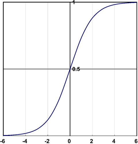
LR is an algorithm derived from regression analyses that form a linear relationship between different features by means of coefficients. This popular ML algorithm was initially borrowed from statistics. The regression output is passed through a mathematical function that produces the probability of occurrence of Landslides. The name logistic regression is derived from the logistic function or sigmoid function (Figure 5), which is the core element of this algorithm. According to this function, when the value of any variable x is positive, the function sets off an asymptote to the line$y\mathrm{ }=\mathrm{ }1,$ and similarly, for negative values of $x,$ an asymptote $y\mathrm{ }=\mathrm{ }0$ is set. LR can be considered as a special case of a generalized linear model (McCullagh and Nelder 1989), used to get results in binary form.

Figure 5. The logistic function or sigmoid function.

This parametric model is able to predict the solutions of a problem, using the concept of probability, and hence it is actively used for LSM. The algorithm finds a fitting function, to establish a non-linear relationship with the landslide and non-landslide points and the input layers. LR does not require hyper parameter tuning and hence can be used easily in predictive models like LSM. The equation used by LR, to find the probability of occurrence of landslide ($P$) using the input layers can be expressed as: (5) $$P\mathrm{ }=\frac{e^z}{1+e^z}$$(5) where z is a linear fitting function, using the different input layers, which can be expressed as (6) $$z\mathrm{ }=\mathrm{ }{a}_0\mathrm{ }+a_1{X}_1\mathrm{ }+a_2{X}_2\mathrm{ }+\cdots +\mathrm{ }{a}_n{X}_n\mathrm{ }$$(6) where $a_0$ is the intercept, $a_1,a_2\dots \dots \dots \mathrm{ }{a}_n\mathrm{ }$ are the regression coefficients and $X_1,\mathrm{ }{X}_2,\dots \dots .X_n$ are the landslide conditioning factors, obtained from the input layers. LR can be efficiently used for getting satisfac factory predictions if the dependent variable is in binary form and the input data set is sufficiently large with minimum duplicates and little multicollinearity.

3.2.3. K-Nearest neighbors

KNN as the name implies, is an algorithm that works by seeing the characteristics of neighboring data values. KNN is one of the simplest ML algorithms which has wide applications and is being used in LSM for a decade (Marjanovic et al. 2009). The algorithm predicts a membership probability for each class, which indicates the probability of a given element can be allocated to any class (Bröcker and Smith 2007). For classifying an object, the algorithm observes KNN falling in the radius of the object. The algorithm takes a poll of all neighbors and assigns the class, which has got the maximum number of votes. The object will be classified as to how the maximum number (K) of its nearest neighbors are classified. The value of K is a small positive integer, given as a parameter, and a change in k value might affect the results of the algorithm (Figure 6).

Figure 6. Graphical representation of K nearest neighbors algorithm.

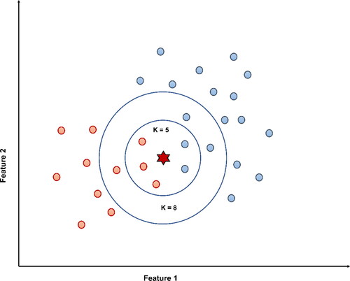
In KNN, the learning is deferred till a request is made, unlike the eager learning algorithms. Hence, it is termed as a ‘lazy’ supervised algorithm. The computations of the algorithm do not depend upon the data distributions and hence it is classified as a non-parametric model. This is an advantage in case of LSM, when the number of features is high, and the data is seldom fit to neat distributions. The algorithm receives an unclassified dataset, and it computes the distance from each data point, to determine the K closest neighbors (Figure 5). The labels of the K closest neighbors are then used for voting and classification of the data point.

3.2.4. Random Forest

RF is an ensemble algorithm. Just like a forest is created by many trees, this algorithm works with a combination of many Decision Trees (DT) (Figure 7). A DT has nodes and branches, the nodes make the decision to continue on a particular branch. By taking consecutive decisions, including all the features, the DT decides which class to assign to an object. The RF takes into account decisions of specified K number of trees. It calculates the probability of landslide occurrence on the basis of votes. Each tree in a RF contains a subset of the whole dataset, which is independently sampled by means of bootstrapping (Breiman et al. 2006). RF in LSM is well known to provide highly accurate results owing to the random selection at each node.

Figure 7. Graphical representation of RF algorithm.

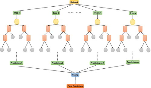
RF algorithms can also decrease the overfitting issues by building several trees, bootstrapping and splitting of nodes. As the tree grows, the randomness of the model is also increasing. While splitting a node, the algorithm does not quest for the most vital feature, but for the best one among the random subset of features. This diversity results in a better model and it can be fine-tuned by changing the maximum number of features taken at each node, the depth of trees and number of trees to be combined.

3.2.5. Support vector machines

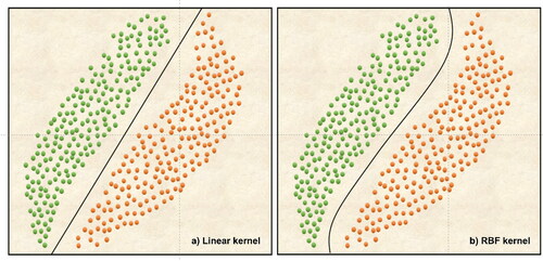
The support vector machines (SVM) algorithm finds a hyperplane in a multidimensional space, which can classify the distinct data point. Hyperplanes can be termed as the decision boundaries that aid in classifying the data point (landslides and no landslides in this case). The dimension of the hyperplane alters according to the number of layers used for LSM. It is possible that multiple hyperplanes can be used to classify the data points. Hence, the purpose of the SVM algorithm is to choose a hyperplane with maximum margin or maximum distance between the data points of both classes using the statistical learning theory (Cortes and Vapnik 1995). Maximum margin is chosen to accommodate the possible data points that may be added in the future. Those data points which are nearer to the hyperplane determine the position and orientation of hyperplanes and are called as support vectors.

The required outputs in SVM are obtained by using different kernel functions, which transform the input data into the required forms (Cristianini and Schölkopf 2002). The choice of the right kernel function is critical in the prediction performance of the model. Linear, radial basis function (RBF), polynomial and sigmoid are some of the kernel functions employed in SVM. The localized and finite response of the RBF kernel has made it the most popular in LSM applications. The difference between two kernel functions, linear and RBF, is shown in Figure 8. Even though both kernels can be used to define the hyperplane in figure, RBF kernel can provide a classifier with a higher margin.

Figure 8. Graphical representation of SVM algorithm.

3.3. K-fold cross-validation

Cross-validation can be defined as a resampling technique used to assess the performance of ML models with a limited dataset. In k-fold cross-validation, the input is a single parameter k, which defines the number of groups or fold the data is divided into. Cross-validation is used in ML, to know the performance of a model on the unseen data. The method is simple and provides a less biased estimate of the skill scores of the ML model.

The procedure of k-fold cross-validation technique includes dividing the dataset into k groups (folds) of equal size (Figure 9). Out of the k-folds, k-1 sets are taken for training the model and the remaining 1 set for testing the performance of the model. The process is repeated k-1 times more, so that each set of data is considered as a test set.

Figure 9. Graphical representation of k-fold validation.

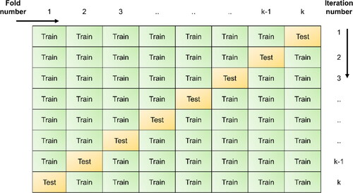
Many studies have used k-fold cross-validation for LSM and most of the studies follow 10-fold cross-validation (Sun et al. 2020) and some of them have used fivefold cross-validation (Palamakumbure et al. 2015). However, these numbers are chosen arbitrarily and the effect of the number of folds have not been explored in detail. Rodríguez et al. (2010) points out that a lesser number of k (k = 2) can be used for the comparison of different ML algorithms, due to the lower variance. It is said that when a single algorithm is used, k = 5 or k = 1 0 are recommended, however, if computationally feasible, repeated cross-validation shall be conducted (Rodríguez et al. 2010).

3.4. Performance evaluation of the models

The performance of ML models considered in this study is compared using the accuracy values and receiver-operating characteristic (ROC) curves approach. The comparison of different models can be done using a confusion matrix, in which the probabilities estimated by each model are compared with the presence or absence of landslide points in the test dataset. Accuracy of a model can be computed as the ratio of the correct predictions to the total data points in the test dataset. Based on the attributes attained from the confusion matrix, the true positive rate ($\mathrm{TPR}$) and the false positive rate ($\mathrm{FPR}$) of the model can be calculated. $\mathrm{TPR}$ is the ratio of appropriately predicted landslide points to the total count of landslide points in the test dataset and $\mathit{FPR}$ is the ratio of incorrect landslides predicted, to the total count of nonlandslide points in the test dataset. The following equations are used for the calculation of accuracy, $\mathrm{TPR}$ and $\mathrm{FPR}:$ (7) $$\mathrm{Accuracy}\mathrm{ }=\frac{\mathrm{TP}+\mathrm{TN}}{\mathrm{TP}+\mathrm{FN}+\mathrm{FP}+\mathrm{TN}}$$(7) (8) $$\mathrm{TPR}\mathrm{ }=\mathrm{ }\frac{\mathrm{TP}}{\mathrm{TP}+\mathrm{FN}}$$(8) (9) $$\mathrm{FPR}\mathrm{ }=\mathrm{ }\frac{\mathrm{FP}}{\mathrm{FP}+\mathrm{TN}}$$(9) where $\mathrm{TP}$ is the true positives, the number of landslides correctly predicted, $\mathrm{FN}$ is the false negatives, the number of landslides missed by the model, $\mathrm{FP}$ is false positives, the number of nonlandslide points in which landslides were incorrectly predicted by the model and $\mathrm{TN}$ is true negatives, the correctly predicted non-landslide points. For a perfect model, the TPR value should be 1 and FPR value should be zero. The plot between these two is known as the ROC curve, and the area under this curve (AUC) is used for comparing the performance of each model. The method is widely used for quantitative comparison of performance of different models (Chen et al. 2021; Li et al. 2021). ROC curves are plotted for each value of k in cross-validation, for each ML model for both 12.5 m and 30 m resolution. The best performing model is then chosen to develop the landslide susceptibility map for Idukki.

4. Results

The performance of all the machine learning models, for different DEM resolutions and different number of folds in cross-validation were carried out using the AUC approach. To enhance the performance of KNN, RF and SVM, the hyper parameters were fine tuned. The ROCs for fine-tuned models are shown in Figure 10.

Figure 10. ROC curves using different ML algorithms: a) NB, b) LR, c) KNN, d) RF, and e) SVM.

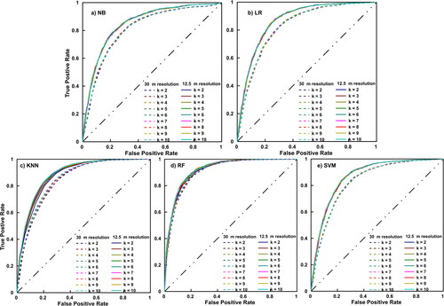
The NB algorithm showed a clear distinction between the results of 12.5 m and 30 m DEMs, while the different values of k did not have much consequence on the model performance (Figure 10a). The maximum AUC was obtained at k = 7 (AUC = 0.848) for 12.5 m resolution and the minimum value was obtained as 0.807, for 30 m resolution, when k = 3. The values of AUCs were varying from 0.807 to 0.810 for 30 m resolution and from 0.846 to 0.848 in the case of 12.5 m resolution. The standard deviation of AUC values in each fold is found to be less in 12.5 m resolution. The value starts from 0.002 when k = 2 and increases to 0.157 in when k = 10. For 30 m resolution, the values vary from 0.005 to 0.020 as the value of k increases from two to ten.

The AUC values obtained using LR algorithm were found to be higher than those with NB, in all the cases. Similar to the case of NB, the results of 30 m and 12.5 m were clearly distinct, but the AUCs obtained by a different number of folds were found to be very close to each other (Figure 10b). Even though there was no significant increase in the AUC values with respect to the number of folds, the maximum value was obtained as 0.867 for both k = 7 and k = 10. While comparing both these models, it can be observed that the standard deviation is almost four times for k = 10 (0.0190) when compared with that at k = 7 (0.005). The best performing model using LR was chosen as the one with 12.5 m resolution and k = 7, considering both the values of AUC and standard deviation. The maximum AUC obtained in the case of 30 m resolution was 0.810 for both k = 7 and k = 10, while the minimum value of AUC obtained in the case of 12.5 m resolution was 0.865 when k = 3.

In KNN algorithm, the key parameter is the number of neighbors, K. The value of K was first fine-tuned for both 12.5 m and 30 m resolutions. The hyper parameter tuning was conducted for 12.5 m and 30 m separately and the best value of K was obtained as 9 and 15, respectively. The AUC values for a different number of folds were then carried out using the fine-tuned parameters. The AUC values obtained using KNN were found to be higher than those obtained using NB in all cases and were slightly higher than to those obtained using LR. Unlike LR and NB, the AUCs for different number of folds are not very close in the case of KNN. The maximum value of AUC was obtained as 0.888 when k = 9 for 12.5 m resolution and the minimum value was 0.840 when k = 2, with 30 m resolution.

RF is widely used for LSM, and the findings of this study also support RF as a good tool for LSM. The AUC values obtained using RF method are higher than all the other algorithms. It should also be noted that the AUC values for 30 m resolution obtained using RF are also higher than those obtained from all other algorithms. The major limitation of RF model is the requirement of hyper parameter tuning. The number of estimators, maximum depth of trees and minimum samples at each split were fine tuned for 30 m and 12.5 m resolution separately as 200, 20, 2 and 400, 25, 2, respectively. The tuned parameters were then used for finding out the effect of several folds. All AUC values obtained using RF algorithm are above 0.900, with the minimum value 0.902 for 30 m resolution with two folds and maximum value 0.920 for 12.5 m resolution with seven folds. The standard deviation is also less when compared with other models. The AUC values slightly differ from each other, with respect to the number of folds (Figure 10d).

The most crucial criteria in deciding the performance of an SVM is the selection of suitable kernel function. After multiple trials, RBF kernel was chosen as the suitable one to classify the dataset used in this study. SVM also needs hyper parameters tuning, and the c value and gamma value were fine tuned for the two different resolutions considered. The c value calibrated for both resolutions was obtained as 1000, while the value of gamma was obtained as 0.0001 for 12.5 m and 0.001 for 30 m resolution. The AUC values for SVM were similar to those of LR and are slightly lesser than those obtained using KNN. As in the case of LR, the distinction between 12.5 m and 30 m resolutions is clear, but the AUC curves for a different number of folds overlap with each other (Figure 10e). The maximum value of AUC attained using SVM is 0.867, for 12.5 m resolution and 5 folds cross-validation. The AUC values are almost constant from k = 5 to k = 10, but the standard deviation increases from 0.015 to 0.019. The standard deviations for all trials using SVM were found to be higher than the other algorithms.

Next, the landslide susceptibility maps were plotted using the best performing models developed using each algorithm (Figure 11) and were evaluated in detail to understand the percentage distribution of spatial probability of occurrence of landslides in Idukki (Figure 12). The area is divided into five categories (very-low, low, medium, high and very-high) according to the probability of occurrence of landslides.

Figure 11. Best performing landslide susceptibility maps developed using different algorithms: a) NB, b) LR, c) KNN, d) RF, and e) SVM.

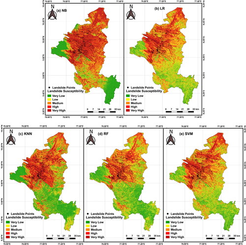
Figure 12. Percentage distribution of total pixels and landslide pixels for the best performing landslide susceptibility maps developed using different algorithms: a) NB, b) LR, c) KNN, d) RF, and e) SVM.

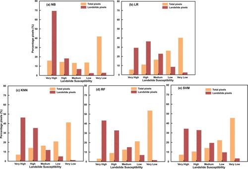
The ratio of pixels in each category, to the total number of pixels is depicted as total pixels percentage, and the ratio of number of landslides that happened in each category, to the total number of landslides considered, is the landslide pixels percentage. The maximum number of pixels belongs to very-low category in all cases (Figure 12). The distribution is almost uniform among the other four categories in the case of NB. For all other algorithms, the percentage pixels increase with a decrease in probability of occurrence of landslides.

It can be understood from Figure 12 that the maximum number of landslides in all cases, except LR, has occurred in the pixels with very-high probability of landslides. Among all the five, the best performing model is the one developed using RF (Figure 11d), in which 4.40% of the total area is classified with very-high susceptibility, 10.53% with high susceptibility, 13.14% with medium susceptibility, 19.83% with low susceptibility and 52.08% with very-low susceptibility. In this case, the maximum number of landslides (43.29%) have occurred in locations classified with very-high susceptibility and only 1.62% of the events have happened in locations with very-low susceptibility. The effect of each conditioning factor on landslide susceptibility was evaluated in detail for the best performing model, which clearly indicates how the spatial resolution of DEM has affected the model performance.

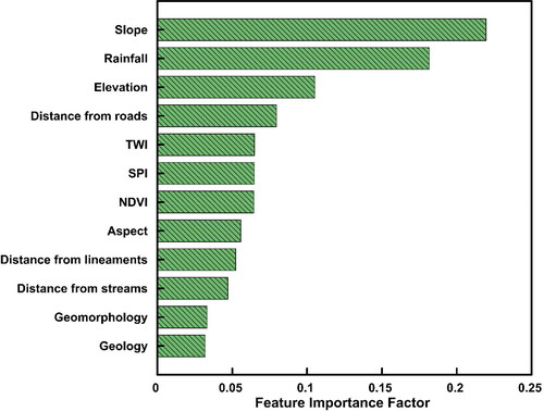
From the best performing model derived using RF, it can be understood that the probability of occurrence of landslides is highly influenced by the slope of the region, with an importance factor of 0.220 (Figure 13). From Figure 4, it is evident that slope values are highly influenced by the resolution of DEM. The rainfall is the next crucial factor with importance factor 0.182 and then comes the elevation with importance factor 0.105. Distance from roads is also a crucial factor, as most of the landslides happen very close to the roads cut through the hillsides, without proper lateral support. The three different indices considered, TWI, SPI and NDVI, were found to have very close importance factors, 0.649, 0.647 and 0.644, respectively. The values of TWI and SPI were found to be more important than the distance from streams. Geology and geomorphology were the least important features with a value of importance factor 0.031 and 0.033, respectively, in this study. The importance factors imply the relevance of using suitable DEM for LSM. The different conditioning factors like elevation, slope, TWI, SPI and aspect are derived from DEM, and all these layers are having high importance factors. Thus, the quality of a majority of layers depends upon the quality of DEM.

Figure 13. Feature importance factors for the best performing model.

The evaluation indicates that the landslide susceptibility map derived using RF model with 12.5 m resolution and 7-fold cross-validation can be used as a reliable tool by the planners and policy makers for making decisions regarding future developments. The impending risk due to landslides in Idukki must be controlled by minimizing further development activities in very-high susceptible zones where the maximum number of landslides are reported. Rainfall is one critical feature which cannot be controlled manually, but any alteration to the features like slope, elevation, TWI, SPI, NDVI, aspect through large-scale land use modifications should be strictly controlled. Strengthening existing road cuttings, and effective planning of future roads according to the susceptibility maps can also control the number of landslides along the road corridors.

5. Discussion

From the results, the best performing model in case of all algorithms was obtained at a resolution of 12.5 m. While comparing the variation in accuracy and AUC values with respect to the number of folds for each algorithm as shown in Figure 14, it is clear that the resolution of DEM has influenced the performance of NB, LR and SVM algorithms. There is a remarkable increase in the performance indicators of these three algorithms when 12.5 m DEM is used. In the case of KNN, the minimum accuracy improved from 0.765 to 0.799 upon the usage of a finer resolution DEM, but the variation between maximum accuracy obtained by 30 m resolution and the minimum accuracy obtained by 12.5 m resolution is marginal. The values are 0.777 and 0.799, respectively (Figure 14). In the case of RF algorithm, this difference is further less. The results of KNN and RF algorithms indicate the significance of data splitting. The maximum accuracy obtained using 30 m resolution is higher that obtained by 12.5 m resolution, by varying the number of folds used for cross-validation, or in other words, by changing the ratio of train to test dataset in the case of RF algorithm. The performance of 7-, 8-, 9-, and 10-fold cross-validations with 30 m resolution was better than 2- and 3-fold cross-validations using 12.5 m resolution, as observed from Figures 10 and 14.

Figure 14. Comparison of minimum and maximum values of: a) accuracy; and b) AUC obtained for 12.5 m and 30 m resolutions.

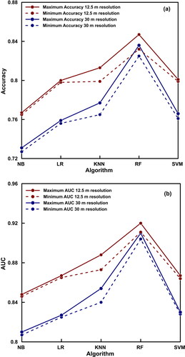
The general trend is an increasing accuracy with respect to the number of folds for lesser values of k; i.e., when more data is used for training, but the optimum performance was obtained for different algorithms at different values of k (Table 1). Figure 14 shows that there is no notable increase in the accuracy and AUC values of NB, LR and SVM algorithms with respect to the values of k. The accuracy of RF algorithm improved from 0.830 to 0.847 in the case of 12.5 m resolution and from 0.825 to 0.836 in the case of 30 m resolution as mentioned in Table 1. In the case of KNN, the accuracies improved from 0.799 to 0.813 and from 0.765 to 0.777 in the case of 12.5 m and 30 m resolution, respectively. From the analysis, all algorithms are performing better with 12.5 m resolution DEM. The maximum accuracy is obtained for RF with 7 folds, as 0.847 when the resolution is 12.5 m.

Table 1. Comparison of accuracy and AUC values for different algorithms using 12.5 m resolution DEM.

Algorithm	Accuracy ± SD	AUC ± SD	Optimum value of number of folds
NB	0.767 ± 0.012	0.848 ± 0.006	7
LR	0.800 ± 0.010	0.867 ± 0.006	7
KNN	0.813 ± 0.012	0.888 ± 0.006	9
RF	0.847 ± 0.012	0.920 ± 0.001	7
SVM	0.801 ± 0.007	0.867 ± 0.010	5

The comparison of different algorithms shows that the choice of a suitable algorithm is the most crucial factor in LSM. The performance is highly influenced by the algorithm and the response of each algorithm to the variation in spatial resolution and the number of folds is different. The accuracy values are the highest in the case of RF algorithm and the least in the case of NB. The assumption of NB algorithm that the predictor variables are independent highly affects the prediction performance of the model. This assumption has a significant effect on the results and the chances of less accurate results are higher when the parameters are not independent. The values of LR and SVM are comparable, while the accuracies obtained by KNN are slightly higher when compared with LR and SVM. LR algorithm results in lesser performance when the problem is non-linear; and the algorithm does not provide good results when the parameters are mutually related. The advantage of using LR is that it does not require any hyper parameter tuning. Even though RF is providing the highest accuracies, complex models like SVM and RF involve higher computational time due to the hyper-parameter tuning. The variation in accuracy values with respect to the number of folds is relevant in the case of KNN and RF only. The statistical performance of the models can be further enhanced by employing ensemble learning using single or hybrid models (Dou et al. 2019; Pham et al. 2020). While comparing the different algorithms, it can be noticed that the optimum value of k is obtained as same for both 30 m and 12.5 m resolution in all cases. Thus, the best suited number of folds depends upon the number of data points and algorithm, rather than the resolution of data.

The study shows that RF algorithm performs better than all the other algorithms considered, in all the cases. The findings of the study point towards the significance of the choice of DEM resolution and data splitting for LSM. The resolution of DEM clearly affects the data in all DEM derived layers and hence the importance of all conditioning factors, which in turn affects the performance of ML model. However, the results indicate that finer resolution data does not indicate better performance. The performance is also influenced by the choice of algorithm and ratio of data splitting. The study proves that the performance of RF algorithm is affected by both the resolution of DEM and number of folds. The important concern here is while using RF algorithm, the wrong selection of train to test ratio might result in poor performance, even with a higher resolution DEM.

The representation of landslides may affect the prediction performance of data driven approaches. However, studies have shown that single point data can satisfactorily represent landslides and different sampling strategies are less significant with the use of advanced algorithms (Dou et al. 2020; Pham et al. 2020). Hence, this aspect is not discussed in this manuscript. With the availability of better resolution DEMs, the performance can be further improved, and the study points out that if computational facilities are available, the performance should be evaluated for different train to test ratios, to obtain the best model. When the resolution of LSM is finer, it helps in efficient management and planning, but the study shows that in the case of RF algorithm (the best performing one), finer resolution does not always guarantee better results. Random choice of the value of number folds might yield poor results irrespective of the resolution of the dataset. Hence, for each study area, the best suited algorithm, spatial resolution and train to test ratio shall be selected after thorough study, as the choice can significantly affect the performance of the derived landslide susceptibility map.

6. Conclusion

Landslide susceptibility maps for Idukki district in southern part of India were developed using five different machine learning algorithms viz. NB, LR, KNN, RF and SVM. Twelve conditioning factors were used to develop the models at two different resolutions, 12.5 m and 30 m k-fold cross-validation were used to assess the performance. The effect of data splitting was also evaluated by varying the number of folds used in k-fold cross-validation from 2 to 10.

The landslide susceptibility maps were plotted for the best performing models using each algorithm, to understand in detail the spatial distribution of probability of occurrence of landslides. The total area was classified into five categories, based on landslide susceptibility. As per the best model developed using RF, 4.40% of the total area is classified with very-high susceptibility, 10.53% with high susceptibility, 13.14% with medium susceptibility, 19.83% with low susceptibility and 52.08% with very-low susceptibility landslide zones. The slope, rainfall and elevation were found to be the most critical features deciding the occurrence of landslides in Idukki.

The analysis showed that the resolution has a significant effect on the performance of model, and the 12.5 m resolution models were performing better than the 30 m resolution models using all the algorithms. The effect of data splitting was found to be significant in KNN and RF algorithms and was negligible in the case of all other algorithms. The standard deviations of the results were the least for a smaller number of folds and it increases along with the number of folds. The optimum performance was obtained for k values 7, 7, 9, 7 and 5 for NB, LR, KNN, RF and SVM, respectively. The ROC curve approach was used to compare the performance of different algorithms and the maximum value of AUC was obtained as 0.920, for RF model with k value 7 and 12.5 m resolution. The results indicate that the spatial resolution has a significant effect on the prediction performance of all algorithms, while the best performing algorithms are also influenced by the number of folds. Hence, if computational facilities are available, it is advised to develop landslide susceptibility maps, by comparing the performance of datasets using available DEM resolutions and different train to test ratios.

Disclosure statement

The authors declare no conflict of interest.

Data availability

Raw data were generated at Indian Institute of Technology, Indore. Derived data supporting the findings of this study are available from the corresponding author [Biswajeet Pradhan] on request.

Additional information

Funding

This research is funded by the Centre for Advanced Modelling and Geospatial Information Systems (CAMGIS), Faculty of Engineering and Information Technology, the University of Technology Sydney, Australia. This research is also supported by Researchers Supporting Project number RSP-2021/14, King Saud University, Riyadh, Saudi Arabia.

References

- Abraham MT, Pothuraju D, Satyam N. 2019. Rainfall thresholds for prediction of landslides in Idukki, India: an empirical approach. Water. 11(10):2113.
- Abraham MT, Satyam N, Reddy SKP, Pradhan B. 2021. Runout modeling and calibration of friction parameters of Kurichermala debris flow, India. Landslides. 18(2):737–754.
- Abraham MT, Satyam N, Rosi A, Pradhan B, Segoni S. 2021. Usage of antecedent soil moisture for improving the performance of rainfall thresholds for landslide early warning. Catena. 200(January):105147.
- Abraham MT, Satyam N, Shreyas N, Pradhan B, Segoni S, Abdul Maulud KN, Alamri AM. 2021. Forecasting landslides using SIGMA model: a case study from Idukki, India. Geomat Nat Hazards Risk. 12(1):540–559.
- Akgun A. 2012. A comparison of landslide susceptibility maps produced by logistic regression, multi-criteria decision, and likelihood ratio methods: a case study at İzmir, Turkey. Landslides. 9(1):93–106.
- Akgun A, Türk N. 2010. Landslide susceptibility mapping for Ayvalik (Western Turkey) and its vicinity by multicriteria decision analysis. Environ Earth Sci. 61(3):595–611.
- ASF DAAC. 2015. Alaska Satellite Facility Distributed Active Archive Center (ASF DAAC) Dataset: ASF DAAC 2015, ALOS PALSAR_Radiometric_Terrain_Corrected_high_res; Includes Material © JAXA/METI 2007.
- Bai SB, Wang J, Zhang FY, Pozdnoukhov A, Kanevski M. 2008. Prediction of landslide susceptibility using logistic regression: a case study in Bailongjiang River Basin, China. Proc – 5th Int Conf Fuzzy Syst Knowl Discov FSKD. 4:647–651.
- Breiman L, Last M, Rice J. 2006. Random Forests: finding Quasars. In: Stat challenges astron. New York: Springer; p. 243–254.
- Bröcker J, Smith LA. 2007. Increasing the reliability of reliability diagrams. Weather Forecast. 22(3):651–661. https://journals.ametsoc.org/doi/https://doi.org/10.1175/WAF993.1.
- Bui DT, Ho T-C, Pradhan B, Pham B-T, Nhu V-H, Revhaug I. 2016. GIS-based modeling of rainfall-induced landslides using data mining-based functional trees classifier with AdaBoost, Bagging, and MultiBoost ensemble frameworks. Environ Earth Sci. 75(14):1101. http://link.springer.com/https://doi.org/10.1007/s12665-016-5919-4.
- Bui DT, Pradhan B, Lofman O, Revhaug I, Dick OB. 2012. Landslide susceptibility assessment in the Hoa Binh province of Vietnam: a comparison of the Levenberg–Marquardt and Bayesian regularized neural networks. Geomorphology. 171–172:12–29. https://linkinghub.elsevier.com/retrieve/pii/S0169555X12002061.
- Capitani M, Ribolini A, Bini M. 2013. The slope aspect: a predisposing factor for landsliding? Comptes Rendus – Geosci. 345(11–12):427–438. https://doi.org/http://dx.doi.org/10.1016/j.crte.2013.11.002.
- Catani F, Lagomarsino D, Segoni S, Tofani V. 2013. Landslide susceptibility estimation by random forests technique: sensitivity and scaling issues. Nat Hazards Earth Syst Sci. 13(11):2815–2831.
- Chen Y, Chen W, Janizadeh S, Bhunia GS, Bera A, Pham QB, Linh NTT, Balogun A-L, Wang X. 2021. Deep learning and boosting framework for piping erosion susceptibility modeling: spatial evaluation of agricultural areas in the semi-arid region. Geocarto Int. 1–27. https://www.tandfonline.com/doi/full/https://doi.org/10.1080/10106049.2021.1892212.
- Chen Z, Ye F, Fu W, Ke Y, Hong H. 2020. The influence of DEM spatial resolution on landslide susceptibility mapping in the Baxie River basin, NW China. Nat Hazards. 101(3):853–877.
- Cortes C, Vapnik V. 1995. Suppport vector networks. Mach Learn. 20(3):273–297.
- Cristianini N, Schölkopf B. 2002. Support vector machines and kernel methods: the new generation of learning machines. AI Mag. 23(3):31–41.
- Department of Mining and Geology Kerala. 2016. District Survey Report of Minor Minerals. Thiruvananthapuram.
- Dikshit A, Satyam DN. 2018. Estimation of rainfall thresholds for landslide occurrences in Kalimpong, India. Innov Infrastruct Solut. 3(1). Article number: 24. doi: https://doi.org/10.1007/s41062-018-0132-9
- Dou J, Yunus AP, Bui DT, Merghadi A, Sahana M, Zhu Z, Chen CW, Han Z, Pham BT. 2020. Improved landslide assessment using support vector machine with bagging, boosting, and stacking ensemble machine learning framework in a mountainous watershed, Japan. Landslides. 17(3):641–658.
- Dou J, Yunus AP, Bui DT, Merghadi A, Sahana M, Zhu Z, Chen CW, Khosravi K, Yang Y, Pham BT. 2019. Assessment of advanced random forest and decision tree algorithms for modeling rainfall-induced landslide susceptibility in the Izu-Oshima Volcanic Island, Japan. Sci Tot Environ. 662:332–346.
- Dou J, Yunus AP, Merghadi A, Shirzadi A, Nguyen H, Hussain Y, Avtar R, Chen Y, Pham BT, Yamagishi H. 2020. Different sampling strategies for predicting landslide susceptibilities are deemed less consequential with deep learning. Sci Tot Environ. 720(February):137320.
- Dou J, Yunus AP, Tien Bui D, Sahana M, Chen C-W, Zhu Z, Wang W, Pham BT. 2019. Evaluating GIS-based multiple statistical models and data mining for earthquake and rainfall-induced landslide susceptibility using the LiDAR DEM. Remote Sens. 11(6):638.
- Formetta G, Capparelli G, Versace P. 2016. Evaluating performance of simplified physically based models for shallow landslide susceptibility. Hydrol Earth Syst Sci. 20(11):4585–4603.
- Froude MJ, Petley DN. 2018. Global fatal landslide occurrence from 2004 to 2016. Nat Hazards Earth Syst Sci. 18(8):2161–2181. https://nhess.copernicus.org/articles/18/2161/2018/.
- Geological Survey of India. 2010. Geology and minerals: District Resource Map, Idukki. [place unknown].
- Gilewski P. 2021. Impact of the grid resolution and deterministic interpolation of precipitation on rainfall–runoff modeling in a sparsely gauged mountainous catchment. Water. 13(2):230. https://www.mdpi.com/2073-4441/13/2/230.
- Hao L, van Westen C, Martha TR, Jaiswal P, McAdoo BG, Rajaneesh A. 2020. Constructing a complete landslide inventory dataset for the 2018 monsoon disaster in Kerala, India, for land use change analysis. Earth Syst Sci Data. 12(4):2899–2918. https://essd.copernicus.org/articles/12/2899/2020/.
- Jaya IGNM, Ruchjana BN, Abdullah AS, Andriyana Y. 2021. Comparison of IDW and GP models with application to spatiotemporal interpolation of rainfall in Bali Province, Indonesia. J Phys Conf Ser. 1722(1). Article number is : 012080
- Jones S, Kasthurba AK, Bhagyanathan A, Binoy BV. 2021. Landslide susceptibility investigation for Idukki district of Kerala using regression analysis and machine learning. Arab J Geosci. 14(10):838. https://link.springer.com/https://doi.org/10.1007/s12517-021-07156-6.
- Kanungo DP, Singh R, Dash RK. 2020. Field observations and lessons learnt from the 2018 landslide disasters in Idukki District, Kerala. Curr Sci. 119(11):1797–1806.
- Lary DJ, Alavi AH, Gandomi AH, Walker AL. 2016. Machine learning in geosciences and remote sensing. Geosci Front. 7(1):3–10. https://doi.org/http://dx.doi.org/10.1016/j.gsf.2015.07.003.
- Li Y, Chen W, Rezaie F, Rahmati O, Davoudi Moghaddam D, Tiefenbacher J, Panahi M, Lee M-J, Kulakowski D, Tien Bui D, et al. 2021. Debris flows modeling using geo-environmental factors: developing hybridized deep-learning algorithms. Geocarto Int. 1–25. https://www.tandfonline.com/doi/full/https://doi.org/10.1080/10106049.2021.1912194.
- Lima P, Steger S, Glade T. 2021. Counteracting flawed landslide data in statistically based landslide susceptibility modelling for very large areas: a national-scale assessment for Austria. Landslides (December 2020). 18(11):3531–3546. https://link.springer.com/https://doi.org/10.1007/s10346-021-01693-7.
- Luti T, Segoni S, Catani F, Munafò M, Casagli N. 2020. Integration of remotely sensed soil sealing data in landslide susceptibility mapping. Remote Sens. 12(9):1486. https://www.mdpi.com/2072-4292/12/9/1486.
- Marjanovic M, Bajat B, Kovacevic M. 2009. Landslide susceptibility assessment with machine learning algorithms. In: 2009 Int Conf Intell Netw Collab Syst. Barcelona Spain: IEEE; p. 273–278. http://ieeexplore.ieee.org/document/5368960/.
- McCullagh P, Nelder JA. 1989. Generalized linear models. 2nd ed. London, New York: Chapman and Hall.
- Meena SR, Ghorbanzadeh O, van Westen CJ, Nachappa TG, Blaschke T, Singh RP, Sarkar R. 2021. Rapid mapping of landslides in the Western Ghats (India) triggered by 2018 extreme monsoon rainfall using a deep learning approach. Landslides. 18(5):1937–1950. http://link.springer.com/https://doi.org/10.1007/s10346-020-01602-4.
- Merghadi A, Yunus AP, Dou J, Whiteley J, ThaiPham B, Bui DT, Avtar R, Abderrahmane B. 2020. Machine learning methods for landslide susceptibility studies: a comparative overview of algorithm performance. Earth Sci Rev. 207(June):103225.
- Miner A, Vamplew P, Windle DJ, Flentje P, Warner P. 2010. A comparative study of various data mining techniques as applied to the modeling of landslide susceptibility on the Bellarine Peninsula, Victoria, Australia. In: 11th IAEG Congr Int Assoc Eng Geol Environ. Auckland, New Zealand; p. 1327–1336.
- National Remote Sensing Centre 2015. Cartosat DEM. Natl Remote Sens Centre, Dep Space, Gov India.
- Palamakumbure D, Flentje P, Stirling D. 2015. Consideration of optimal pixel resolution in deriving landslide susceptibility zoning within the Sydney Basin, New South Wales, Australia. Comput Geosci. 82:13–22. https://doi.org/http://dx.doi.org/10.1016/j.cageo.2015.05.002.
- Pham BT, Nguyen-Thoi T, Qi C, Phong T, Van Dou J, Ho LS, Le H, Van, Prakash I. 2020. Coupling RBF neural network with ensemble learning techniques for landslide susceptibility mapping. Catena. 195(June):104805.
- Pham BT, Pradhan B, Tien Bui D, Prakash I, Dholakia MB. 2016. A comparative study of different machine learning methods for landslide susceptibility assessment: a case study of Uttarakhand area (India). Environ Model Softw. 84:240–250. https://doi.org/http://dx.doi.org/10.1016/j.envsoft.2016.07.005.
- Pham BT, Prakash I, Dou J, Singh SK, Trinh PT, Tran HT, Le TM, Van Phong T, Khoi DK, Shirzadi A, et al. 2020. A novel hybrid approach of landslide susceptibility modelling using rotation forest ensemble and different base classifiers. Geocarto Int. 35(12):1267–1292.
- Piciullo L, Calvello M, Cepeda JM. 2018. Territorial early warning systems for rainfall-induced landslides. Earth Sci Rev. 179(April 2017):228–247.
- Pourghasemi HR, Pradhan B, Gokceoglu C, Mohammadi M, Moradi HR. 2013. Application of weights-of-evidence and certainty factor models and their comparison in landslide susceptibility mapping at Haraz watershed, Iran. Arab J Geosci. 6(7):2351–2365. http://link.springer.com/https://doi.org/10.1007/s12517-012-0532-7.
- Pradhan B. 2013. A comparative study on the predictive ability of the decision tree, support vector machine and neuro-fuzzy models in landslide susceptibility mapping using GIS. Comput Geosci. 51:350–365. https://doi.org/http://dx.doi.org/10.1016/j.cageo.2012.08.023.
- Pradhan B, Sameen MI. 2017. Effects of the spatial resolution of digital elevation models and their products on landslide susceptibility mapping. In: Pradhan B, editor. Laser scanning appl landslide assess. 1st ed. Cham: Springer International Publishing; p. 133–150. http://link.springer.com/https://doi.org/10.1007/978-3-319-55342-9.
- Qiu J, Wu Q, Ding G, Xu Y, Feng S. 2016. A survey of machine learning for big data processing. EURASIP J Adv Signal Process. 67 (2016). https://doi.org/https://doi.org/10.1186/s13634-016-0355-x
- Reichenbach P, Rossi M, Malamud BD, Mihir M, Guzzetti F. 2018. A review of statistically-based landslide susceptibility models. Earth-Sci Rev. 180:60–91. https://linkinghub.elsevier.com/retrieve/pii/S0012825217305652.
- Rodríguez JD, Pérez A, Lozano JA. 2010. Sensitivity analysis of kappa-fold cross validation in prediction error estimation. IEEE Trans Pattern Anal Mach Intell. 32(3):569–575.
- Singh SK, Taylor RW, Rahman MM, Pradhan B. 2018. Developing robust arsenic awareness prediction models using machine learning algorithms. J Environ Manage. 211:125–137.
- Sorbino G, Sica C, Cascini L. 2010. Susceptibility analysis of shallow landslides source areas using physically based models. Nat Hazards. 53(2):313–332.
- Sun D, Xu J, Wen H, Wang Y. 2020. An optimized random forest model and its generalization ability in landslide susceptibility mapping: application in two areas of three Gorges Reservoir, China. J Earth Sci. 31(6):1068–1086.
- Vishnu CL, Sajinkumar KS, Oommen T, Coffman RA, Thrivikramji KP, Rani VR, Keerthy S. 2019. Satellite-based assessment of the August 2018 flood in parts of Kerala, India. Geomat Nat Hazards Risk. 10(1):758–767. https://www.tandfonline.com/doi/full/https://doi.org/10.1080/19475705.2018.1543212.
- Wang W, He Z, Han Z, Li Y, Dou J, Huang J. 2020. Mapping the susceptibility to landslides based on the deep belief network: a case study in Sichuan Province, China. Nat Hazards. 103(3):3239–3261.
- van Westen CJ, van Asch TWJ, Soeters R. 2006. Landslide hazard and risk zonation – why is it still so difficult? Bull Eng Geol Environ. 65(2):167–184.
- Yalcin A. 2008. GIS-based landslide susceptibility mapping using analytical hierarchy process and bivariate statistics in Ardesen (Turkey): comparisons of results and confirmations. Catena. 72(1):1–12.
- Youssef AM, Al-Kathery M, Pradhan B. 2015. Landslide susceptibility mapping at Al-Hasher area, Jizan (Saudi Arabia) using GIS-based frequency ratio and index of entropy models. Geosci J. 19(1):113–134. http://link.springer.com/https://doi.org/10.1007/s12303-014-0032-8.
- Zare M, Pourghasemi HR, Vafakhah M, Pradhan B. 2013. Landslide susceptibility mapping at Vaz Watershed (Iran) using an artificial neural network model: a comparison between multilayer perceptron (MLP) and radial basic function (RBF) algorithms. Arab J Geosci. 6(8):2873–2888. http://link.springer.com/https://doi.org/10.1007/s12517-012-0610-x.
- Zhou L, Pan S, Wang J, Vasilakos AV. 2017. Machine learning on big data: opportunities and challenges. Neurocomputing. 237(December 2016):350–361.