Mudslide susceptibility assessment based on a two-channel residual network

Abstract

In response to the challenges posed by rugged terrain in Yunnan, hindering large-scale mudslide screening efforts, this article introduces a dual-channel Convolutional Neural Network (CNN) constructed using elevation data from historical mudslide-prone valleys (Digital Elevation Model, DEM) and remote sensing imagery. The network is designed to facilitate the comprehensive assessment of potential mudslide hazards in gullies, serving as a crucial tool for early mudslide disaster warning. The model initially employs an enhanced residual structure to extract fundamental features from both types of data. Subsequently, it leverages the SE module and deep separable structure to emphasize the importance of relevant features and expedite model convergence. Finally, the model classifies the gullies under evaluation based on their similarity to gullies where mudslides have previously occurred. Experimental results demonstrate the model’s robust performance in assessing mudflow-prone gullies, achieving an impressive precision rate of up to 81.10% and a recall rate of 82.76%. When applied to evaluate the potential hazard of mudslide gullies across the entirety of Nujiang Prefecture, the model predicts that 87.80% of the mudslide locations are at an extremely high risk. These findings underscore the viability of utilizing image-based gully feature analysis for assessing the hazard levels of mudslide-prone gullies.

Keywords:

• Mudslide
• remote sensing
• convolutional neural network
• hazard evaluation

C.I.C. CLASSIFICATION NUMBER:

• P954

DOCUMENT IDENTIFICATION CODE:

• A

1. Introduction

Mudslides are one of the most common geological hazards in mountainous areas of China (Song et al. 2014). They are a geological phenomenon formed by a combination of internal geological factors and external environmental factors, and often pose a great threat to the local natural environment and human life (Hou et al. 2021). Therefore, a reasonable and effective evaluation of the risk of mudslides is of great significance for disaster prevention and mitigation in mountainous areas. The prevention and control of mudslides first began in the 1960s, and early mudslide studies relied on fieldwork, using statistical analysis in conjunction with field data (Iverson et al. 1997). Common research methods now include statistical theory-based, numerical simulation-based and machine learning-based.

The traditional statistical method is to assess the susceptibility of mudslides by counting various parameters of historical mudslides and fitting the relationship between these parameters using specific functions; there are various such methods, and the common ones are hierarchical analysis (Gu et al. 2023), fuzzy evaluation (Yang et al. 2011), entropy method (Lombardo et al. 2016), gray correlation analysis (Yang 2020), etc. However, statistical theory-based methods typically necessitate the prior selection of specific factors. Given the varying geological conditions across regions, the chosen factors may diverge. Moreover, even when the same method is applied within a single area, different factors may be employed. For instance, in the context of gully hazard assessment in Wenchuan County, Yang (Yang et al. 2018) and Wang (Wang et al. 2017) respectively utilized sediment recharge length ratio and gully density as assessment indicators. The primary reason for such variability lies in the inherent subjectivity in factor selection among different experts. This factor-driven subjectivity hampers the broad applicability of such methodologies, particularly in the context of large-scale land survey endeavors.

The numerical simulation method entails selecting a kinetic model, inputting the precise details and physical parameters of the mudslide gully into the model for computational analysis, and subsequently assessing the gully’s hazard based on the parameters derived from the simulation. Commonly used tools for this purpose include FLO-2D (Genevois et al. 2022), MassFlow (Qiao et al. 2020), FLO-3D (Huang et al. 2022), Debris2D (Wu et al. 2013), and others. Numerical simulation methods face a significant challenge, requiring not only statistical parameters such as main ditch length and slope but also field-acquired information, such as catchment point locations. However, obtaining these data, particularly in topographically complex mountainous regions, often proves to be a formidable task. Consequently, this approach is typically limited in its applicability, as it can only be feasibly employed for the assessment of a handful of gullies. This limitation presents a substantial obstacle when attempting to swiftly evaluate the hazard potential of hundreds or even thousands of gullies.

Machine learning-based approaches involve utilizing statistically or computationally obtained gully factors as training data, followed by optimizing model parameters through backpropagation. Subsequently, the fine-tuned model is applied to assess the risk of mudslide gullies. Methods such as BP Neural Networks (Liu et al. 2020), Multi-Classification Support Vector Machines (Li et al. 2010), and Random Forest Models (Pal et al. 2022) have been explored for gully mudslide hazard assessment. Despite their impressive nonlinear fitting capabilities, manual selection of factors for hazard assessment remains a necessity.

In recent years, with the emergence of Convolutional Neural Networks (CNNs), numerous researchers have embraced their application within the realm of geohazards. CNNs possess the unique ability to dynamically extract salient features from input images, circumventing the need for arduous feature extraction processes and consistently delivering robust recognition results. For instance, some researchers have successfully employed CNNs in landslide susceptibility assessments (Hakim et al. 2022; Yang et al. 2022; Youssef et al. 2022).

However, an extensive literature survey reveals a conspicuous scarcity of research endeavors applying CNNs to the realm of mudslides. This dearth of exploration can be attributed, in part, to the inherent challenges posed by mudslide studies. Mudslides inherently present a limited data pool, making it a small-sample problem fraught with data scarcity. Consequently, rapid and accurate identification of mudslide gullies becomes a formidable challenge. Moreover, the nature of the data itself poses a significant hurdle. The expeditious classification of mudslides using CNNs hinges primarily on Digital Elevation Model (DEM) data and remote sensing data. These two data sources encompass distinct information facets, and directly feeding both into the network training process compromises the precision of the classification.

To surmount these challenges, we draw inspiration from the concept of the Dual-Channel Convolutional Neural Network (Barzinpour and Taki 2018; Han et al. 2022), and propose a Dual-Channel Improved Residual Structure Network (DCRNet). DCRNet facilitates the independent processing of DEM data and remote sensing data, effectively mitigating the adverse effects arising from direct input of both data types into the network. Notably, it eliminates the need for the a priori specification of factors used for hazard assessment. Additionally, the input data for the model comprise continuous image data, as opposed to isolated statistical values, rendering a more comprehensive reflection of gully characteristics. DCRNet, adept at adaptively excavating features from diverse data sources and deciphering inter-feature relationships, offers a comprehensive evaluation of the potential mudslide hazard associated with gullies.

Furthermore, the Dual-Channel Improved Residual Structure Network (DCRNet) introduced in this study represents a novel approach in mudslide research. By overcoming the challenges of limited data and information diversity, DCRNet provides a more accurate and reliable tool for mudslide hazard assessment. The innovation of this method lies in its ability to not only eliminate the need for a priori factor selection, as required by traditional methods but also intelligently extract features from multiple data sources to conduct an in-depth analysis of the potential hazard of gullies. This not only aids in a better understanding of the mechanisms behind mudslide formation but also offers a new approach to address mudslide risks in a wider geographical context.

In this research, Nujiang Prefecture has been selected as a classical high-incidence area for mudslides. Notably, there is a paucity of comprehensive literature pertaining to mudslide hazard studies in this region on a regional scale. Furthermore, it is pertinent to highlight that the climatic and geological conditions prevailing in Nujiang Prefecture bear similarity to other regions prone to high mudslide occurrences, such as Nepal and Pakistan (Xu and Wang 2022). Consequently, the research methodology advanced in this article holds the potential for application in these geographically analogous regions.

The structure of this paper is as follows: first, we will present an exposition on the climatic characteristics specific to the study area; second, a comprehensive delineation of the experimental data and methodologies employed will be expounded; and finally, we will proffer our conclusions and furnish in-depth analyses, all rooted in the outcomes of our experiments.

2. Study area and data sources

2.1. Study area

The Nujiang Lisu Autonomous Prefecture, hereinafter referred to as Nujiang Prefecture, is situated in the northwestern region of China’s Yunnan Province. Its nomenclature is derived from the Nujiang River, which courses through the entirety of the prefecture from north to south. Geographically, the region exhibits distinctive features. In the upper reaches, the terrain is characterized by gentle mountains, shallow river valleys, and extensive lakes and marshes, with the exception of towering snow-capped peaks. Transitioning to the middle reaches, the landscape is dominated by the formidable Hengduan Mountains, marked by rugged terrain, steep peaks, and swiftly flowing rivers. Tributaries on both sides of the main river cascade vertically, often featuring imposing waterfalls, treacherous rapids, and a landscape dotted with numerous waterfalls and precarious shores. Moving downstream, influenced by increased rainwater recharge, the mountains gradually yield to an open expanse, forming an agricultural area.

The climate of Nujiang Prefecture is characterized by its uniqueness, blending the attributes of a low-latitude plateau monsoon climate and three-dimensional climatic influences. The annual average precipitation in the region totals 1,301.9 millimeters, with the primary flood season typically concentrated between May and October, contributing to approximately three-quarters of the total annual precipitation. The month of highest precipitation averages 214.1 mm.

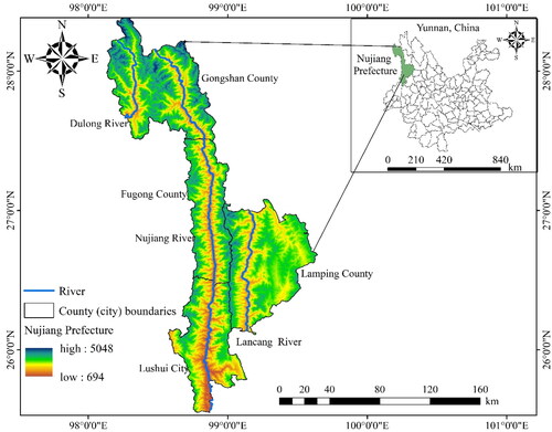
The Nujiang River basin hosts a rich biodiversity, relatively less disturbed by human activities (Zhang et al. 2023). Water temperature displays a remarkable vertical continuity, closely mirroring variations in air temperature (Qiu et al. 2022). Consequently, the overall topography and geomorphological features of Nujiang Prefecture remain relatively stable. The rugged high mountains, steep slopes, extensive river networks, and diverse geological formations collectively provide a nurturing environment conducive to the formation of mudslides. The convergence of intense precipitation and various contributing factors has resulted in the recurrent incidence of mudslide disasters in Nujiang Prefecture (Xu et al. 2023). For a visual representation of the geographical location and topographic distribution of Nujiang Prefecture, please refer to Figure 1 below.

Figure 1. Schematic diagram of the study area.

2.2. Data sources

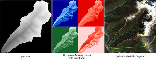
This study utilized Digital Elevation Model (DEM) data and remote sensing data as the primary research datasets. The DEM data were obtained from the publicly available USGS dataset, with a spatial resolution of 30 meters, collected in January 2015. Remote sensing data were exclusively acquired from the Gaofen-1 satellite (GF-1), featuring a resolution of 16 meters and utilizing spectral signals from the blue, red, green, and near-infrared bands. Remote sensing data were acquired over various temporal intervals. For gullies that had previously experienced mudslides, we selected satellite images captured immediately prior to the event. In the case of gullies where mudslides had not yet occurred or were pending assessment, satellite images from November 2022 were employed.DEM data can provide topographic information about the gully, including parameters such as the length of the main gully, catchment area, volume of soil and rock (Zhang et al. 2014), slope, and slope direction (Xie et al. 2011). On the other hand, remote sensing data can furnish surface-related information about the gully, encompassing aspects like surface vegetation coverage, distribution of buildings, and water system conditions (Meyer et al. 2012). These two types of data collectively encompass nearly all the pertinent information about the gully, covering various factors commonly employed in mudslide assessment. Consequently, this article relies on these two datasets.

2.3. Mudslide inventory

In order to adapt the above data to the model in this article, pre-processing of the data was required. First, we distinguished between gullies that had experienced mudslides and those that had not. The processing was as follows: for the valleys where mudslides had occurred, the locations of the mudslides were identified by consulting the Yunnan Disaster Reduction Yearbook and relevant news reports, which pinpointed them to specific villages. Ultimately, 82 gullies in the Nu River basin where mudslides had occurred were identified. For the mudslide valleys that did not occur or were not recorded, the valleys with villages or farmland nearby were selected and recorded using Google Earth’s satellite maps. In this way, we obtained data on 85 valleys with no records of disasters. The 82 gullies where mudslides were confirmed were recorded as positive samples, and the 85 gullies with no disaster records were recorded as negative samples. Once the 167 gullies were identified, ArcGIS was used to determine the location of the gullies, extract the gullies from the DEM map, and then aggregate the extracted gully data. The extracted gullies are illustrated in Figure 2.

Figure 2. Schematic diagram of the gully.

2.4. Data classification criteria

After establishing the positive and negative samples, the experiments categorized them into three groups based on the size of the gully’s watershed area. This division into three categories is supported by a body of research demonstrating a strong correlation between watershed area size and gully hazard (Chen et al. 2020;Liu and Chen 2012;Zhu et al. 2014). These findings underscore the pivotal role played by watershed area size in governing mudslide formation; larger watershed areas are associated with a heightened mudslide risk (Yao et al. 2019). In this article, we classify watershed areas into three categories: small, medium, and large. Correspondingly, positive and negative samples are also divided into these three categories. Positive samples are designated as 0, 1, or 2 based on their watershed area size, while negative samples are labeled as 3, 4, or 5 according to their respective watershed area sizes. The detailed classification method is presented in Table 1.

Table 1. How the sample was classified.

Watershed area (${\mathit{\text{km}}}^2$)	Number of positive samples (pcs)	Number of negative samples (pcs)
Small (1–10)	9 (Class 0)	8 (Class 0)
Medium (10–35)	51 (Class 1)	23 (Class 1)
Large (35–100)	22 (Class 2)	54 (Class 2)

Due to the varying dimensions of DEM images and remote sensing imagery for gullies, with the largest pixel size being 1079*1095, standardizing their dimensions would result in some loss of important feature information. In order to align with the overall network training process and preserve data feature information to the maximum extent possible, all images were uniformly padded to a size of 1280*1280 pixels.

After classifying the positive and negative samples, an imbalance in the sample data based on the watershed area size was identified. To improve the predictive accuracy of these gullies’ hazard levels, all image data were further augmented through rotation and flipping before model training. Detailed results are presented in Table 2.

Table 2. Detailed results of data enhancement.

Category	0	1	2	3	4	5
Pre-enhancement	9	51	22	8	23	54
After enhancement	45	51	44	48	46	54

The number of positive samples increased to 140 and the number of negative samples increased to 148 after the data enhancement process, creating a total of 288 samples. Next, we divided the training and test sets in the ratio of 9:1, 8:2 and 7:3 according to the common data ratio division method of deep learning.

3. Network model DCRNet

3.1. Experimental flow design

Convolutional neural networks are usually trained using a back propagation algorithm. The algorithm evaluates the difference between the predicted and true values of the model by calculating a loss function and uses back propagation to pass the error forward layer by layer from the last layer to update the parameters in the model. After the parameters are updated, the network again undergoes the process of forward and backward propagation, iterating until the error is reduced to an acceptable range, at which point the training of the model is complete. The core operations of a convolutional neural network are formulated as follows: (1) $$Y_{\mathit{\text{out}}}=f_i\left(b_{i,j}+\mathit{\text{conv}}\left(X_{\mathit{\text{in}}},W_{i,j}\right)\right)$$(1) where $Y_{\mathit{\text{out}}}$ and $X_{\mathit{\text{in}}}$ represent the network’s output and input, respectively, $f_i$ stands for the activation function of the ith layer, $b_{i,j}$ corresponds to the jth bias term of the ith layer, and $W_{i,j}$ represents the jth convolution kernel of the ith layer.

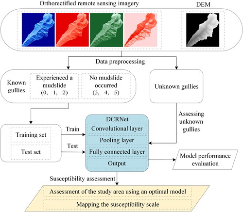
After categorizing the positive and negative samples based on the watershed area size and completing data augmentation, the processed data is further divided into test and training sets using different ratios. These sets are then input into the network for training. Figure 3 below illustrates the experimental flow.

Figure 3. Experimental flow chart.

3.2. Construction of the model

As the experiment incorporates both DEM and remote sensing data, these two datasets offer distinct insights into the geological conditions. To harness this wealth of information effectively, the experiment devises a two-channel network. This network independently extracts features from each dataset and subsequently consolidates these features. The experimental outcomes are then generated through a fully connected layer. Refer to Figure 4 for a detailed depiction of the model structure.

Figure 4. Model structure diagram.

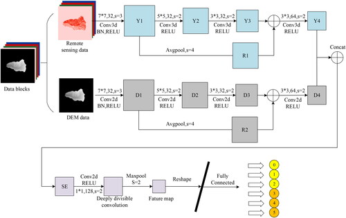
As depicted in Figure 4, the remote sensing maps from the four bands are initially stacked together with the DEM maps, creating a 5-layer data block. During the network training phase, this data block is divided into 1-channel DEM data and 4-channel remote sensing data through slicing. Feature extraction is conducted using a two-channel DCRNet network structure. Each feature extraction channel comprises 4 convolutional layers and 1 residual structure following average pooling (as illustrated in Figure Y1, Y2, Y3, Y4, D1, D2, D3, D4, R1, R2). Subsequent to feature extraction, the resulting feature map Y4 is concatenated with D4 through the Concat function.

To encourage local information interaction within the channel and preserve crucial features, an SE (Squeeze-and-Excitation) attention mechanism is reapplied after feature fusion. Additionally, a depth-divisible convolution is introduced to decrease parameter computation. Finally, the classification outcomes for gullies are generated via a pooling layer and fully connected layer.

Throughout the entire training process, the crux lies in the feature extraction component. Given the constrained volume of experimental data, to mitigate potential overfitting issues and enhance network performance, the experiment introduces 4 convolutional layers to judiciously limit network depth. Furthermore, an improved residual structure with average pooling is employed, effectively addressing the overfitting problem while simultaneously bolstering network performance.

Additionally, recognizing the attributes of multi-channel remote sensing data, three-dimensional convolution is leveraged for feature extraction from the remote sensing data. The resultant feature map, Y4, adeptly encapsulates spatial information.

1. Based on an improved residual structure

   To enhance the classification function for improved accuracy and tackle the optimization challenges in training deeper networks, this article introduces a residual structure (He et al. 2016) for network optimization. Differing slightly from the traditional residual structure, the experimentally designed residual structure replaces the shortcut connection with a global average pooling operation. This operation computes the average feature value within the receptive field and uses it as the output. This modification preserves a greater amount of feature information in the image. Figure 5 illustrates the improved residual structure.

   Assuming that the of layer input $i$ is $x_i,$ the output obtained after the convolutional layer is $F(x_i),$ and the total output after concatenation through residuals is (2) $$y_i=F\left(x_i\right)+x_i$$(2) And the improved residual output is (3) $$y_i=F\left(x_i\right)+H\left(x_i\right)$$(3)

2. Channel attention mechanism and depth-separable convolution

   To diminish the influence of irrelevant features at the edges of input image data while emphasizing the importance of more relevant features, the SENet (Squeeze-and-Excitation Network) structure was incorporated into the experiments (Hu et al. 2018). The SENet structure aims to enhance the network’s expressive power through feature extraction across channel dimensions, ultimately improving network performance. Figure 6 provides a schematic representation of the SENet structure.

Figure 5. Diagram of the improved residual structure.

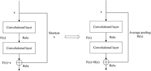
Figure 6. SENet structure diagram.

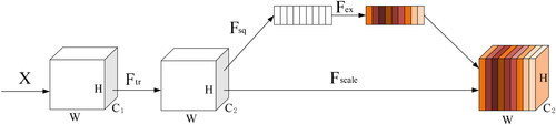
The input image X is initially transformed into a one-dimensional sequence of real numbers via the mapping function $F_{\mathit{\text{tr}}},$ employing the compression operation $F_{\mathit{\text{sq}}}.$ Subsequently, computational demands are reduced through the excitation operation $F_{\mathit{\text{ex}}}.$ Finally, the deflation function $F_{\mathit{\text{scale}}}$ is applied to multiply the weight values of each channel with the corresponding feature values, thereby extracting high-order feature information from the mudslide image.

To mitigate the computational demands on the operating environment and storage, particularly as network depth increases, this article introduces the Depth Divisible Convolutional (DSC) structure (Zhang et al. 2019). DSC achieves this by decoupling the correlation between spatial and channel dimensions, thereby reducing the number of parameters required for convolutional computation and enhancing network efficiency. Figure 7 below provides an illustration of the deeply divisible convolution structure.

Figure 7. Deeply divisible convolutional structure diagram.

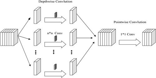
Assuming the input feature map is of size H × W×M, the convolution kernel size is C × C×M, and there are N convolutional kernels, the computational effort for normal convolution is H × W×C × C×M × N, where one convolution operation is needed at each spatial location of the feature map. In contrast, depthwise convolution consists of the computational efforts of Depthwise Convolution (H × W×C × C×M) and Pointwise Convolution (H × W×M × N), resulting in a total computation of H × W×C × C×M + H × W × M × N. It’s evident that the computational load of Depthwise Convolution is significantly lower than that of standard convolution. Furthermore, the two separate convolution operations in Depth Divisible Convolution increase nonlinearity and further enhance the network’s capacity to capture image features.

3.3. Improved loss function

In this article, the model training begins with the utilization of the Cross-Entropy loss function. The Cross-Entropy loss function can be expressed as: (4) $${\mathit{\text{CE}}}_p=-\sum _{i=1}^n{x}_i\mathrm{\text{log}}\hspace{0.17em}{P}_i,i=0,1,2,3,4,5$$(4)

The experiment is categorized into six classes, where $n$ represents the number of categories. $x_i$ serves as the label, indicating that $x_i$ equals 1 if the predicted category is $i,$ otherwise, it is set to 0. $P_i$ represents the neural network’s output, signifying the probability of the category being $i.$ However, the Cross-Entropy loss function tends to bias the network toward learning easily classifiable samples, resulting in suboptimal performance when dealing with small samples. Due to the initial imbalance in the categorized samples, to mitigate the impact of sample imbalance on the model, the experiment introduces an additional loss function known as Focal Loss (FL). FL is designed to address the imbalance in sample categorization by assigning greater weight to hard-to-classify samples, thus emphasizing the training process on these challenging instances. Consequently, this article combines the Focal Loss function with the Cross-Entropy loss function to formulate a new loss function, which is applied to the accurate prediction of potential hazards in different morphological gullies. The Focal Loss function for 6-class classification is as follows: (5) $${\mathit{\text{FL}}}_p=-\alpha \sum _{i=1}^n{\left(1-p_i\right)}^{\gamma }\mathrm{\text{log}}\hspace{0.17em}{p}_i,i=0,1,2,3,4,5$$(5)

In this context, $\alpha$ is a parameter designed to address the sample imbalance issue, and $\gamma$ is a parameter used to manage the challenge of imbalanced samples’ difficulty. $n$ represents the number of categories, while $P_i$ represents the probability value of a correct sample prediction. This study primarily focuses on the sample imbalance problem. Therefore, we fix the value of $\gamma$ at 2 and perform experiments by adjusting the parameter $\alpha .$ Experimental results indicate that setting $\alpha$ to 0.25 leads to a significant improvement in model accuracy when using the combined loss function. The accuracy is approximately 10% higher than when exclusively employing the cross-entropy function. Consequently, the experiment has ultimately determined the loss function as: (6) $${\mathit{\text{Loss}}}_P={\mathit{\text{CE}}}_p+{\mathit{\text{FL}}}_P$$(6)

4. Analysis of results

4.1. Comparative experiments and model performance

This section presents the experimental comparison results between the model proposed in this article and other models using different training and test set division ratios. The hardware used for the experiment includes a CPU: Intel Xeon E5-2650 v3, Memory: 128GB, GPU: NVIDIA GeForce RTX 3090. The software stack consists of Ubuntu 18.06, PyTorch 1.9.0, Python 3.8, and CUDA 11.1.

In this experiment, the dataset is divided into positive and negative samples, resulting in 6 channels, and the DCRNet is employed as the backbone architecture for feature extraction. The hyperparameters are configured as follows: learning rate (lr) = 0.0001, Focal Loss parameter ($\alpha$) = 0.25, dropout rate = 0.5, batch size = 8, and the number of training epochs = 100. The loss function utilized is the joint loss function (${\mathit{\text{Loss}}}_P$), and the optimization method is Stochastic Gradient Descent (SGD).

In multiclassification problems, commonly used evaluation metrics include Accuracy, Precision, Recall, F1-Score, and Kappa, which can be calculated based on the confusion matrix. The following three tables provide performance comparison results between DCRNet and common deep learning models (including VGG, ResNet18, ResNet34, ResNeXt, EfficientNet, and RegNet) in the context of 6-class classification. The "2-classification accuracy" represents accuracy when considering only positive and negative samples. All metrics are results obtained from 10 parallel experiments and averaged.

Based on the results presented in Tables 3–5, it is evident that DCRNet outperforms other network structures in gully feature recognition. As the number of test samples increases, the overall performance of all models tends to decrease. DCRNet consistently exhibits superior performance in gully feature extraction, and its higher recall rate suggests that the model designed in this article is more accurate in capturing features from positive samples.

Table 3. Experimental results for (9:1) training test set division.

Backbone	Precision	Recall	F1 Score	Kappa	Test2_acc	Test6_acc
VGG	0.667	0.614	0.621	0.597	0.690	0.638
ResNet18	0.706	0.638	0.646	0.647	0.759	0.724
ResNet34	0.705	0.631	0.602	0.646	0.724	0.724
ResNeXt	0.695	0.661	0.647	0.634	0.759	0.707
EfficientNet	0.572	0.587	0.478	0.507	0.690	0.483
RegNet	0.510	0.525	0.502	0.402	0.621	0.586
DCRNet	0.811	0.828	0.784	0.772	0.828	0.811

Table 4. Experimental results for (8:2) training test set division.

Backbone	Precision	Recall	F1 Score	Kappa	Test2_acc	Test6_acc
VGG	0.636	0.616	0.614	0.512	0.690	0.621
ResNet18	0.648	0.657	0.630	0.573	0.707	0.699
ResNet34	0.687	0.678	0.664	0.621	0.724	0.698
ResNeXt	0.675	0.651	0.637	0.607	0.698	0.647
EfficientNet	0.659	0.542	0.456	0.599	0.672	0.586
RegNet	0.677	0.633	0.637	0.608	0.690	0.655
DCRNet	0.728	0.713	0.710	0.671	0.741	0.724

Table 5. Experimental results for (7:3) training test set division.

Backbone	Precision	Recall	F1 Score	Kappa	Test2_acc	Test6_acc
VGG	0.616	0.566	0.537	0.537	0.686	0.570
ResNet18	0.741	0.640	0.630	0.691	0.733	0.640
ResNet34	0.749	0.684	0.679	0.701	0.721	0.698
ResNeXt	0.673	0.654	0.653	0.609	0.709	0.651
EfficientNet	0.578	0.617	0.546	0.498	0.721	0.605
RegNet	0.612	0.620	0.613	0.532	0.709	0.640
DCRNet	0.730	0.724	0.723	0.676	0.744	0.721

Despite DCRNet having a relatively small number of network layers compared to VGG and the ResNet series, its performance is improved. This can be attributed to two possible reasons. Firstly, the experiment’s dataset is small, comprising only 288 samples, and deep network structures are prone to overfitting issues when trained on small datasets, leading to suboptimal results. Shallow networks, in this case, tend to perform better. Secondly, DCRNet separately extracts features from DEM and remote sensing data before fusing them. This approach is more effective compared to conventional network structures that directly input all data together, allowing DCRNet to better extract the fundamental features of gullies.

Analyzing the results further, it was found that the best network performance was achieved when the training and test sets were divided in a 9:1 ratio. To provide a more intuitive comparison of all models’ performance, Figure 8 displays a graph illustrating the accuracy of all models under the 9:1 training-test division ratio. The graph showcases the results from the best round of experiments out of 10 parallel sets.

Figure 8. Accuracy curve.

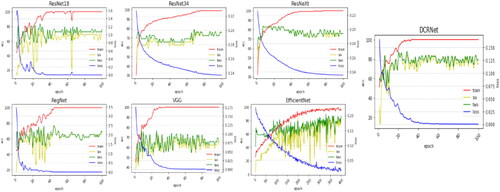
From the figure, it is clear that the performance of the residual series networks doesn’t vary significantly, with test set accuracy hovering around 75%. RegNet and VGG exhibit relatively lower performance, fluctuating between 60% and 70% accuracy. EfficientNet displays more variability in test set accuracy, with the model gradually converging after approximately 300 rounds of training. In contrast, DCRNet performs exceptionally well, achieving network convergence between rounds 30 and 40, with test set accuracy stabilizing at around 80%. These results in Figure 8 underscore that DCRNet excels in classifying gully data with greater accuracy compared to other network architectures.

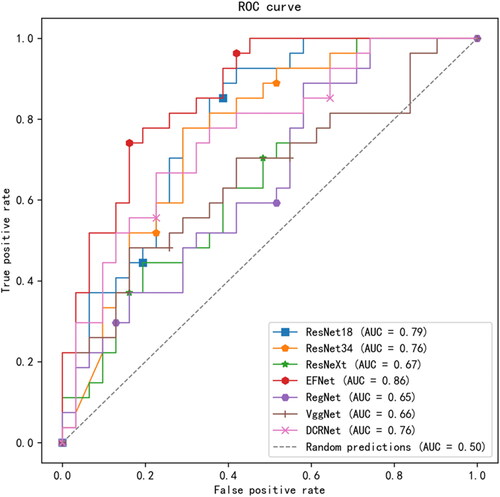
In this section, the Receiver Operating Characteristic curve (ROC) is employed as an alternative evaluation measure to assess the model’s performance. The accuracy of the model is determined by the Area Under the Curve (AUC) metric. The range of AUC values is between 0.5 and 1.Where a higher AUC value indicates a greater model accuracy. Figure 9 below illustrates the ROC curves for the seven models mentioned above. ResNet18, ResNet34, EfficientNet, and DCRNet al.l exhibit AUC values exceeding 0.7, showcasing outstanding capability in distinguishing between positive and negative instances. On the other hand, ResNeXt, RegNet, and VGGNet have AUC values below 0.7, indicating a moderate level of discriminative ability. However, in terms of model selection, despite the higher AUC values for EfficientNet and ResNet18, both exhibit significant fluctuations in predictive accuracy, and their average accuracy rates are inferior to that of DCRNet. Therefore, to pursue a more stable and reliable predictive performance, we have chosen DCRNet as the preferred model for assessing debris flow hazards.

Figure 9. Receiver operating characteristic curve.

4.2. Ablation experiments

To further validate the effectiveness of each component of the model’s architecture, ablation experiments were conducted for comparison. The structures of residuals, SE, and DSC were individually added to the base model to assess the impact on the model’s performance. The training set to test set ratio is 9:1. Detailed results are presented in Table 6.

Table 6. Results of ablation experiments.

	Precision	Recall	F1-score	Kappa	Test2_acc	Test6_acc
Basic net	0.598	0.595	0.582	0.518	0.655	0.590
With 3D	0.633	0.667	0.640	0.560	0.679	0.643
With Res	0.774	0.716	0.709	0.675	0.759	0.742
With SE	0.705	0.629	0.627	0.647	0.724	0.638
With DSC	0.595	0.608	0.587	0.512	0.621	0.586
Res + 3D	0.794	0.743	0.735	0.750	0.773	0.760
Res + SE + DSC	0.804	0.838	0.755	0.764	0.828	0.793
DCRNet	0.811	0.828	0.784	0.772	0.828	0.811

From the above table, it is evident that replacing the 2D convolution of the network with 3D convolution, or adding the SE module or residual structure individually, leads to significant improvements in network performance. This improvement may be attributed to the fact that remote sensing data contains 4 latitudinal dimensions, and 3D convolution is better suited for extracting multidimensional features. On the other hand, the residual structure may better adapt to the classification function, resulting in higher classification accuracy, while the SE structure may be enhancing feature extraction in the channel dimension, thereby capturing more feature information.

Although the performance of the model appears slightly degraded after adding the DSC structure, it significantly improves network efficiency. Furthermore, when structures like residuals and SE are combined, there is a notable enhancement in network performance. This could be due to the fusion of advantages from different structures.

4.3. Optimal parameter selection

To further illustrate the impact of hyperparameters on the experiments and determine the optimal model parameters (Zhao 2020), a series of experiments were conducted to test the learning rate and the value of $\alpha$ used in the loss function. The results, averaged from 10 parallel experiments, are presented in Table 7.

Table 7. Experimental results of the loss function.

Classes of loss functions	$\alpha$ Value	6 Classification accuracy rate (%)	2 Classification accuracy rate (%)
Combined loss (CE + FL)	1	0.707	0.741
	0.5	0.776	0.776
	0.25	0.776	0.811
	0.1	0.707	0.707
	0.05	0.793	0.793
	0.02	0.724	0.759
	0.01	0.752	0.759
Cross-entropy	–	0.689	0.655

From Table 7, it is evident that the model achieves superior classification accuracy when the value of $\alpha$ in the joint loss function is set to 0.25. In contrast, using the cross-entropy loss function alone leads to a nearly 10% drop in classification accuracy. This underscores the effectiveness of the joint loss function devised in this article for handling classification tasks with limited samples.

Regarding the findings in Table 8, the network’s classification performance progressively diminishes as the learning rate increases. Moreover, a higher learning rate necessitates more training epochs for convergence, resulting in a slower convergence rate. This phenomenon may be attributed to the modest sample size utilized in the experiment. A higher learning rate can prevent the model from converging to the optimal model parameters and may hinder it from reaching the local optimum.

Table 8. Experimental results for different learning rates.

Learning rate (lr)	6 Classification accuracy rate (%)	2 Classification accuracy rate (%)	Number of convergence rounds
0.0001	0.811	0.828	35
0.0005	0.793	0.828	40
0.001	0.776	0.793	50
0.005	0.759	0.759	70
0.01	0.759	0.759	100

5. Analysis of the susceptibility to mudslides in gullies and valleys in Nujiang Prefecture

5.1. Calculation of potential hazards

Once the model achieved stable performance, saved model parameters were utilized to evaluate all 672 gullies in the Nujiang River. The assessment involved calculating the potential hazards of these gullies based on the degree of feature similarity between the output of the 672 gullies and the gullies of each category obtained during the experiments.

Let the output results from the model be represented as $x_i,$ where $i=0,1,2,3,4,5.$ These results are transformed into probability values using the softmax function. Subsequently, the sum of feature similarity probabilities for positive samples ($S$) is calculated. The corresponding formula is as follows: (7) $$S_i=\frac{e^{x_i}}{{\sum }_{i=0}^5{e}^{x_i}}$$(7) (8) $$S=\sum _{i=0}^2{S}_i$$(8) where $S_i$ represents the probability value of the gully predicted to be the ith category, and $S$ is the sum of the probability values of the positive samples. In this experiment, positive samples refer to the gullies where mudslides have occurred. If the similarity between the sample to be tested and the three types of gullies in the positive sample is higher, it indicates a higher potential hazard for the tested gully.

The similarity results were converted into susceptibility indices by calculating the value of $S$ for all the samples to be tested. Since the value of $S$ is normalized, $S$ ∈ [0,1]. Clearly, the larger the value of $S,$ the higher the susceptibility of the tested gully, and conversely, the lower the susceptibility of the tested gully. This method generates susceptibility indices for all gullies to be tested. Subsequently, all to-be-tested gullies are categorized in terms of hazard using the natural breakpoint method. Finally, different susceptibility zones are determined, and susceptibility zoning maps are created. Detailed results are presented in Section 5.2.

5.2. Map of susceptibility areas

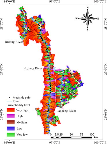
In this section, the susceptibility index for all gullies is statistically determined using the probability distribution calculated by the model. The mudslide susceptibility index is classified into five levels, ranging from high to low, as follows: very high susceptibility zone [0.845,1], high susceptibility zone [0.609,0.845], medium susceptibility zone [0.388,0.609], low susceptibility zone [0.153,0.388], and very low susceptibility zone [0,0.153] (illustrated in Figure 10). Figure 10 reveals that the high susceptibility zone for mudslides is primarily concentrated on both sides of the Nujiang River, encompassing areas such as Fugong County, Gongshan County, Lushui County, and the regions west of the Lancang River. It is also partially concentrated in the Dulong River basin. The overall spatial distribution pattern of high mudflow susceptibility in the study area exhibits a '7′ shape, with a denser concentration of extremely high susceptibility areas in the northwestern part. Meanwhile, the medium and low susceptibility areas are primarily found in the southeastern part of the study area, east of the Lancang River. The combined area of the very high and high susceptibility zones accounts for over 66% of the study area. Notably, the existing mudslide sites roughly align with the extent of the very high and high susceptibility zones.

Figure 10. Map of susceptibility areas.

Additionally, we can observe that within the study area, valleys in the extremely high susceptibility and high susceptibility zones generally exhibit larger and broader characteristics. In contrast, valleys in the low susceptibility and extremely low susceptibility zones tend to be smaller in size. This variation in valley dimensions within the region reflects the combined influence of several geographical, topographical, and climatic factors.The larger size of valleys in the extremely high susceptibility and high susceptibility zones may be linked to a higher prevalence of potential mudslide-contributing factors in these areas. Firstly, regions with significant topographic variations are more likely to witness valley formation, as steep mountainous terrain can lead to more pronounced erosion and sediment transport, resulting in the development of wider valleys. Secondly, these areas may experience more frequent precipitation events, and rainfall-driven erosive processes can contribute to the expansion of valley dimensions. Additionally, land use patterns and vegetation cover conditions may contribute to valley formation and enlargement, with specific land utilization practices and reduced vegetation cover potentially amplifying the presence of mudslide susceptibility factors.Conversely, the smaller size of valleys in the low susceptibility and extremely low susceptibility zones may be attributed to flatter terrain, lower precipitation levels, and reduced erosive forces, which collectively result in smaller valley dimensions. Furthermore, these regions may benefit from improved land management practices and greater vegetation cover, which can help mitigate the presence of mudslide susceptibility factors.

In summary, the relationship between valley size and mudslide susceptibility can be attributed to the intricate interplay of various geographical and environmental factors, collectively shaping the potential mudslide risk in different areas.

5.3. Statistical analysis of susceptibility

To provide a more detailed overview of the results of mudslide susceptibility assessment, Table 9 presents information regarding the number of gullies, elevation differences, slope drop ratios, projected areas, and the number of mudslides corresponding to each susceptibility class for the five susceptibility categories. Additionally, it calculates the ratio of mudslides to the average watershed area of the gullies for each susceptibility class. These data were computed using ArcGIS.

Table 9. Details of different levels of susceptibility.

Models	DCRNet
Susceptibility class zones	Very low	Low	Medium	High	Very high
Total number of gullies	289	109	66	54	154
Average length per gully/$m$	5627.607	6044.822	7511.938	9240.62	14937.41
Total watershed area/${\mathit{\text{km}}}^2$	2510.084	1006.482	821.888	1011.062	7509.177
Average area per gully/${\mathit{\text{km}}}^2$	8.655	9.234	12.644	18.723	49.080
Area share/%	19.52	7.83	6.39	7.86	58.40
Average elevation difference/$m$	1533.768	1658.972	1739.833	2026.204	2378.799
Average longitudinal ratio drop/‰	272.54	274.45	231.61	219.27	159.25
Number of mudslides	2	3	1	4	72
Percentage of mudslides/%	0.69	2.75	1.52	7.41	46.75

Specifically, the elevation difference is obtained by subtracting the elevation of the gully mouth from the highest elevation of the gully. The length of the main gully corresponds to the length of the longest stream, while the gully area is the raster area calculated based on the projected coordinates. The slope-drop ratio, also known as the gully-bed ratio drop, represents the ratio of the elevation difference to the length of the main gully.

From the results in Table 9, it can be visualised that the number of gullies predicted based on the DCRNet model is 154 in the very high susceptibility class. The area of very high susceptibility zone in the study area is about 7509.177 ${\mathit{\text{km}}}^2,$ accounting for 58.40% of the total area of the study area, in which about 87.80% of the mudslide sites are distributed in very high susceptibility class, 4.88% of the sites are distributed in high susceptibility class, and 7.32% of the sites are distributed in medium, low, and very low susceptibility class. The percentage of mudslides in very high susceptibility areas is as high as 46.75 per cent, 7.41 per cent in high susceptibility areas and 4.96 per cent in medium, low and very low susceptibility areas.

In addition, according to the results in the above table, it can also be observed that the average length of gullies and watershed areas in the very high susceptibility areas are much larger than those in other susceptibility classes. In general, according to the order of mudslide susceptibility class from low to high, the values of watershed area, main gully length, and average elevation difference show an increasing trend, i.e. the more susceptible areas tend to have longer main gully, larger watershed area, and larger elevation difference. Figure 11 below visualises the susceptibility zones according to elevation difference, main gully length, gully area and longitudinal ratio drop.

Figure 11. Visualisation of susceptibility zoning.

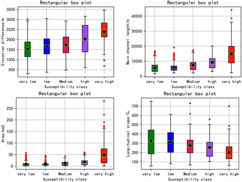
Looking at Figure 11, it becomes evident that areas with higher susceptibility levels, especially the extremely high susceptibility zone, show notable trends in various factors. They tend to have larger differences in elevation, longer main gully lengths, and more extensive watershed areas, indicating a consistent positive correlation. Conversely, the longitudinal slope drop demonstrates a declining pattern, signifying a negative relationship with susceptibility zone levels. A higher longitudinal slope drop suggests steeper terrain, which results in greater variations in elevation within these gullies. However, these gullies typically feature shorter main gully lengths, which enable faster water drainage and reduce the likelihood of debris accumulation and mudslide formation. Hence, gullies with a higher longitudinal slope drop are generally less susceptible to mudslides.

Furthermore, when observing the boxplots related to main gully length and watershed area, several outliers are noticeable. This suggests that the study area tends to have larger geographical areas and longer gullies as common characteristics. Interestingly, the minimum values of watershed areas for different susceptibility levels are nearly identical, indicating that the study area is prone to scenarios where even small gullies can lead to significant disasters. To summarize, gullies in the study area that exhibit a higher susceptibility to mudslides often share characteristics such as larger elevation differences, longer main gully lengths, and more extensive watershed areas.

5.4. Analysis of typical gullies

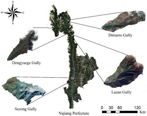
This section combines the analysis related to mudslides at four locations in Dongyuege, Dimaro and Lazan villages in Gongshan County and Sezong village in Lushui City, whose geographical locations are shown in Figure 12.

Figure 12. Schematic diagram of a typical gully.

Dongyuege is situated at 98°43'56.021" E, 27°38'10.331" N, featuring a primary channel length of 10.34 km, an elevation difference of 2.602 km, and an expanse of 17.777 km². The slope ratio is 251.651‰, with an average slope of 23.081°. The terrain is intricate, characterized by soil types encompassing soft thin-layered soil and well-developed, highly active leached soil. The vegetation cover comprises forests, shrublands, and sparse woodlands. Geological formations include granite, gneiss, slate, shale, green schist, and phyllite. Dongyuege encountered a significant mudslide on August 18, 2010, impacting nearly ten thousand individuals and resulting in a direct economic loss of 140 million yuan.

Dimaro is located at 98°70'5.20" E, 27°94'74.80" N, featuring a primary channel length of 6.1 km, an elevation difference of 2.153 km, and an area of 6.559 km². The slope ratio is 352.936‰, with an average slope of 19.911°. The soil comprises well-developed, highly active leached soil, and the vegetation cover includes dry land, shrublands, and sparse woodlands. Geological formations encompass granite, gneiss, slate, shale, green schist, and phyllite. Dimaro experienced a mudslide on July 26, 2019, resulting in the destruction of four production buildings, two fatalities, and one missing person, causing substantial economic losses to the local area.

Lazan Village is positioned at 98°49'46.132" E, 27°32'32.503" N, featuring a primary channel length of 7.824 km, an elevation difference of 2.426 km, and an area of 16.45 km². The slope ratio is 310.082‰, with an average slope of 21.2°. The soil comprises well-developed, highly active leached soil, and the vegetation cover includes forests, shrublands, and sparse woodlands. Geological formations include granite, gneiss, slate, and shale. Lazan Village experienced three mudslides on July 5, 2017, May 31, 2018, and July 10, 2018, respectively. Nearly two thousand people were affected, with a direct economic loss exceeding 25 million yuan.

Sezong Village is situated at 98°89′29.92″ E, 26°38′54.97″ N, featuring a primary channel length of 12.182 km, an elevation difference of 2.527 km, and an area of 26.017 km². The slope ratio is 207.431‰, with an average slope of 18.147°. The soil comprises low-active strong acid soil with humus and well-developed, highly active leached soil. The vegetation cover includes dry land, forested areas, shrublands, sparse woodlands, and moderately covered grasslands. Geological formations encompass granite, gneiss, slate, shale, limestone, and other carbonate rocks. Sezong Village experienced a mudslide on April 23, 2016, resulting in the destruction of one house, two missing persons, 770 affected individuals, and a direct economic loss of 13.6 million yuan.

These four gullies exhibit substantial differences in elevation, characterized by loose soils and sparse vegetation cover. The geological composition is primarily composed of easily weathered rocks, including granite, gneiss, slate, and phyllite. These geological characteristics make these areas highly susceptible to the initiation of mudslides. Furthermore, Gongshan County experiences an annual precipitation range of 2700 to 4700 millimeters, while Lushui City encounters annual precipitation ranging from 2600 to 3800 millimeters. The combination of abundant rainfall and ample sediment sources creates favorable conditions for the occurrence of mudslides.

All four of the above mudslide gullies caused significant economic damage and the following are the similarity scores and susceptibility indices for the four mudslide gullies as assessed by the DCRNet model. These are shown in Table 10.

Table 10. Potential hazards of gullies.

Gully name	Similarity score per category ($x_i$)						Susceptibility Index S
	0	1	2	3	4	5
Dongyuege	0.0002	0.9221	0.0421	0.0000	0.0002	0.0354	0.9644
Dimarro	0.9721	0.0004	0.0001	0.0233	0.0041	0.0000	0.9726
Lazan	0.9868	0.0025	0.0000	0.0004	0.0097	0.0004	0.9893
Sezong	0.0141	0.9598	0.0000	0.0000	0.0034	0.0226	0.9739

As can be seen from Table 10, Dongyege gully and Sezong gully are more similar to the mudslide valleys in category 1, and Dimaro gully and Lazan gully are more similar to the mudslide valleys in category 0. This indicates that all four of these valleys are generally large in size and long in length. In addition, all four valleys have a susceptibility index of 0.95 or more, making them extremely high susceptibility areas. Lazan gully, in particular, has experienced three mudslide events between 2017 and 2018, which further demonstrates the good capability of this experimental model in mudslide assessment.

5.5. Visualisation of network features - Dongyuege gully as an example

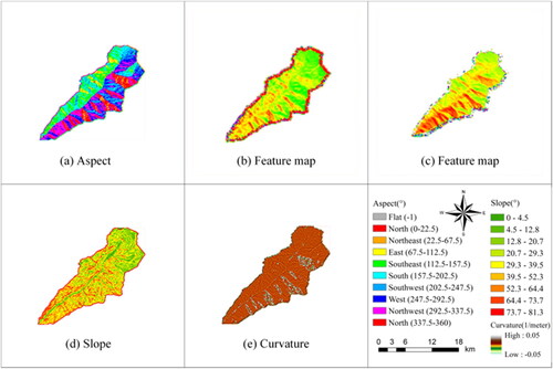
To better visualise the ability of DCRNet to extract gully features, this section shows the feature map after visualisation of the network intermediate layer, using the Dongyuege gully as an example. Figure 13 below shows the gully feature map obtained from the network intermediate layer with the gully image obtained through ArcMap. Where (a), (d) and (e) represent the slope direction, slope and curvature images obtained through ArcMap respectively, while (b) and (c) are the feature maps output by the network intermediate layer. After observation and comparison, it is found that the feature map (b) is very similar to the slope direction image (a), while the Dongyuege gully sit northeast to southwest and are in the northern hemisphere, so the southeast slope is more obvious. This suggests that the network is most likely extracting the slope direction features. In addition, the feature maps show a concentration of colour near the mouth of the gully, while the slope values are larger in the Dongyuege near the mouth of the gully. Therefore, the slope features corresponding to the feature map output from the middle layer of the network also match the actual situation. The curvature is calculated from the slope direction and represents the curvature perpendicular to the direction of maximum slope. It is related to the convergence and dispersion of surface water flows. By observing that some of the features of the feature map are similar to the curvature map, it is possible that the network has also extracted the features of curvature.

Figure 13. Map of slope direction, gradient, curvature and network characteristics.

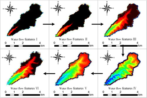
In addition, the visualisation of the middle layer of the network captures two particular features, the first being the change in the area of elevation difference threshold concern, the process of which is shown in Figure 14. As can be seen in the figure, the elevation difference threshold changes continuously from stage I to VI, expanding from 1441 m at the mouth of the gully to 4285 m at the highest point throughout the region, with a progressive increase in elevation difference. The larger elevation difference imparts greater kinetic energy to the water flow, which is highly conducive to the rapid scouring of the water. As can be observed in Figure 15, the convergence of the water flow is a progressive process, starting at the mouth of the gully and gradually spreading throughout the valley and continuously flowing out of the gully mouth. Combining Figure 14 with Figure 15, it can be seen that the convergence of is closely related to the difference in elevation. A large difference in elevation is very conducive to the convergence and acceleration of the water, which gives the water greater kinetic energy and enables it to carry more debris, sediment and other sources to form a mudslide, which is continuously discharged from the mouth of the gully and eventually forms an accumulation area. These features captured by the network visualisation are well illustrated in Figures 14 and 15.

Figure 14. Map of elevation difference threshold intervals.

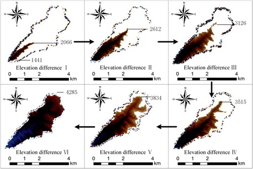
Figure 15. Map of the evolution of the water system.

The upper reaches of Dongyuege ditch are mostly schist, dacite and metasedimentary rocks of the Carboniferous system, while the middle reaches are mostly granite of the late Yanshan period (Li et al. 2021)and the lower reaches are mainly metasedimentary rocks, schist, hornblende and dacite of the Carboniferous system (Lo and Xu 2016). As the Dongyuege ditch is located in the eastern plate of the Nujiang River Rift, the influence of fracture tectonics has led to the development of lamproite, joints and fissures in the watershed, and the resistance to weathering varies greatly (Jie et al. 2015;Wang et al. 2018). In addition, the watershed area in the middle and upper reaches of the Dongyuege gorges is prone to the formation of moraines due to the perennial accumulation of snow. These physical conditions provide favourable conditions for the formation of mudslides. In addition, the data collection combined with the historical mudslide situation shows that since January 2010, the rainfall in Prady Township, Gongshan County, has increased significantly compared to previous years, with 1685.6 mm of rainfall from January to August, 422.8 mm more than the average rainfall of the same period in previous years. The combination of high temperatures in August and the possibility of large amounts of snow and ice melt water in the upper reaches of the Dongyuege, combined with the rich physical conditions of the basin, most likely contributed to the mudslides.

Therefore when the rainy season comes, due to the special situation of the area, it is important to strengthen the monitoring of mudslides, especially the monitoring of weather and rain conditions, and to prepare contingency plans in case of emergency.

6. Discussion and Conclusion

6.1. Feasibility discussion on employing deep learning for mudslide research

In this research, we employed deep learning methodologies to evaluate the susceptibility of debris flows and conducted a comparative analysis of the performance of various classical neural network models. Based on the outcomes presented in Figure 8, residual series networks demonstrated a slightly superior performance on the mudslide dataset, whereas the performance of RegNet and VGG was somewhat less satisfactory. In contrast, although EfficientNet exhibited commendable performance in specific scenarios, its results displayed significant fluctuations and, overall, failed to align with the effectiveness of our designed DCRNet. Residual series networks excelled in capturing the intricate features of mudslides, potentially attributed to the incorporation of residual blocks, thereby facilitating the network in learning and conveying crucial features more effectively. In handling geological and topographic data, the robust feature extraction capability of residual structures appeared more suitable for complex environments, proving pivotal in mudslide research.

EfficientNet manifested substantial variability in certain cases, likely stemming from the complexity of its network structure and sensitivity to parameters. Despite achieving commendable performance on specific datasets, EfficientNet’s results fell short of expectations for highly nonlinear and complex datasets such as mudslide. Moreover, as depicted in the findings presented in Figure 9, DCRNet demonstrated an AUC value of 0.76, indicative of a relatively high level of accuracy. Following a comprehensive comparison of each model’s performance, we concluded that DCRNet exhibited greater robustness in decision-making, particularly in complex geological environments. Consequently, DCRNet was chosen as the experimental network model for our study.

The comparative analysis of our experimental findings with previous studies provides essential validation for the efficacy of our approach. In a study centered on mudslides in Nujiang Prefecture, conventional methods, as exemplified by Kong et al. (2019), employing statistical indicators and the analytic hierarchy process for mudslide hazard assessment, achieved a mere 70% accuracy. In contrast, Wang et al. (2022) utilized a BP neural network, attaining a comparatively modest accuracy of 77.7%. These traditional methodologies may exhibit limitations in capturing intricate geological and topographic features, especially when confronted with highly nonlinear datasets. Conversely, the convolutional neural network (CNN) employed in our study exhibits robust feature extraction capabilities, facilitating the automatic learning of more intricate spatial and temporal features, consequently achieving a heightened predictive accuracy of 82.28%.

From a standpoint of geographical applicability, we have expanded the scope of our research to encompass the entire Nujiang Prefecture. In contrast to the earlier works of Xu and Huang (2015) and Li et al. (2019), which focused solely on specific regions, our study achieved a high predictive accuracy, forecasting 72 out of 82 mudslide points as high-risk, resulting in an accuracy rate of 87.8%. Our model demonstrated superior performance in assessing mudslide susceptibility, highlighting its applicability and generalization capabilities across a broader geographical range. This success can be attributed to the comprehensive impact of multiple factors. Firstly, the widespread distribution of data likely positively influenced the model’s performance. In contrast to prior studies concentrating on limited regions, our research employed a more extensive dataset for training and validation, enabling the model to better learn and comprehend the geological and topographic characteristics of the entire Nujiang Prefecture, thereby enhancing its adaptability to complex geographical environments. Secondly, the diversity of terrain features emerges as a critical factor in the model’s success. Nujiang Prefecture encompasses various terrain types, including high mountains, canyons, and hilly areas, where the geological composition and topographic features may play distinct roles in mudslide formation. The deep learning methodology applied in this study possesses robust feature extraction capabilities, enabling automatic learning and capturing of key features within different terrain types, facilitating the model’s comprehensive adaptation to the geographical complexity of the entire Nujiang Prefecture.

Upon conducting a more in-depth analysis of the mudslide assessment results, we observed a correlation between our research findings and those of a pertinent study (Li et al. 2019). Their results indicated that high and extremely high susceptibility small basins were mainly concentrated west of the Lancang River, including Gongshan County, Fugong County, and Lushui City, while Lanping County was less affected. In comparison, our susceptibility assessment results (as depicted in Figure 10) exhibit a similar distribution pattern, aligning with the spatial distribution of historical mudslide points. Furthermore, in Li Yimin’s study, some regions, such as Dongyuege, were assessed as having low susceptibility, while Lazan was assessed as highly susceptible. However, when considering historical mudslide data, Dongyuege has experienced severe mudslide events, and Lazan had consecutive mudslide occurrences in 2017 and 2018. In contrast, our study, utilizing a CNN model, evaluated both of these valleys as highly susceptible. To some extent, this further underscores the potential accuracy of using CNNs for mudslide susceptibility assessment.

Nonetheless, the CNN model presents certain limitations in terms of interpretability. In the field of disaster analysis, comprehending the interpretability of model results is pivotal. To address this challenge and better showcase DCRNet’s ability to extract features related to mudslide susceptibility, this article employs feature maps from the network’s intermediate layers to interpret key features. By comparing these feature maps with images generated through ArcMap, we observe that CNNs can effectively capture features such as the shape, area, and contours of mudslide valleys. Furthermore, results from Figures 14 and 15 indicate that CNNs can capture not only intuitive features like shape and area but also numerous continuous deep features. For example, they can focus on the evolution of water flow and changes in the threshold area of elevation differences.

In summary, the convolutional neural network (CNN) method employed in this study has not only achieved high methodological accuracy but has also demonstrated significant advantages in geographical applicability across a broader range. It exhibits notable accuracy in susceptibility assessment results. Deep learning methods hold immense potential in the evaluation of mudslide susceptibility. By enhancing the interpretability of the model, a more comprehensive understanding of potential mudslide hazards can be obtained. This approach is not confined to case study regions but can be extended to mudslide research in various global locations.

6.2. Conclusion and way forward

For the prediction and early warning of gully-type mudslides, this article develops a deep learning model based on DEM and remote sensing image data, applying it to assess mudslide susceptibility in gullies within Nujiang Prefecture. This research introduces several noteworthy innovations:

1. Novel Hazard Assessment Approach: This study pioneers a novel method for evaluating the potential hazard of mudslide gullies by employing a deep learning model. This innovation enhances our understanding and predictive capabilities related to mudslide hazards and introduces fresh tools and methodologies for early disaster warning and risk management.

2. DCRNet Model: The article presents the DCRNet model, purposefully designed to utilize mudslide gullies as evaluation units, with DEM and remote sensing data as the primary input. The model employs a dual-channel structure, each channel featuring an enhanced residual structure for improved data feature extraction. This augmentation enables the extraction of more valuable features. Subsequently, these two types of features are fused, enhancing network performance through the SE module and deep separable structures. Finally, an enhanced loss function is applied to minimize the disparity between true and predicted values, thereby improving model accuracy. DCRNet achieved an 82.28% identification rate for mudslide gullies, with an AUC value of 0.76, affirming the feasibility of employing CNN models for potential hazard analysis.

3. Contextual Hazard Analysis: This article employs a CNN model to analyze the potential hazard of mudslide gullies, representing a robust approach. Although the designed model exhibits commendable performance when trained on small samples, there are inherent limitations to enhancement. These limitations may arise from the current incomplete understanding of the contextual and formational mechanisms underlying mudslide occurrences. Additionally, accuracy improvements may be constrained by relying solely on select conditional factors. For instance, rainfall is a pivotal predisposing factor. To potentially achieve superior predictive outcomes, future research may consider quantifying these predisposing factors and integrating them with topographic and geomorphological conditions through multimodal deep learning.

In forthcoming work, we will explore the incorporation of multimodal data fusion to further advance model recognition accuracy and bolster its generalization capabilities.

Author contributions

Conception and methodology, Ruohao Yuan; validation and resources, Yumeng Luo, Xu Wang; writing and editing, Ruohao Yuan, Cunxi Liu; supervision, Baoyun Wang, Fanshu Xu. All authors have read and agreed to the published version of this manuscript.

Data availability statement

The data that support the findings of this study are available from the corresponding author upon reasonable request.

Remote sensing optical images are selected from National Platform for Common Geospatial Information Services and the link is https://www.tianditu.gov.cn/.

DEM data is obtained from Shuttle Radar Topography Mission (SRTM) data and the link is https://lpdaac.usgs.gov/products/srtmgl1v003/.

Disclosure statement

No potential conflict of interest was reported by the authors.

Correction Statement

This article has been corrected with minor changes. These changes do not impact the academic content of the article.

Additional information

Funding

This work was supported by National Natural Science Foundation of China: [Grant Number 61966040].

References

- Barzinpour F, Taki P. 2018. A dual-channel network design model in a green supply chain considering pricing and transportation mode choice. J Intell Manuf. 29(7):1465–1483. doi: 10.1007/s10845-015-1190-x.
- Chen W, Zhao X, Zhang H, Liu T, Li C, Wang K. 2020. Hazard assessment of highway debris flow based on the fuzzy comprehensive evaluation method in Northwest Yunnan. Highway. 65: 25–29.
- Genevois R, Tecca PR, Genevois C. 2022. Mitigation measures of debris flow and landslide risk carried out in two mountain areas of North-Eastern Italy. J Mt Sci. 19(6):1808–1822. doi: 10.1007/s11629-021-7212-6.
- Gu F, Chen J, Sun X, Li Y, Zhang Y, Wang Q. 2023. Comparison of machine learning and traditional statistical methods in debris flow susceptibility assessment: a case study of Changping District, Beijing. Water. 15(4):705. doi: 10.3390/w15040705.
- Hakim WL, Rezaie F, Nur AS, Panahi M, Khosravi K, Lee C-W, Lee S. 2022. Convolutional neural network (CNN) with metaheuristic optimization algorithms for landslide susceptibility mapping in Icheon, South Korea. J Environ Manage. 305:114367. doi: 10.1016/j.jenvman.2021.114367.
- Han R, Jones CK, Lee J, Wu P, Vagdargi P, Uneri A, Helm PA, Luciano M, Anderson WS, Siewerdsen JH. 2022. Deformable MR-CT image registration using an unsupervised, dual-channel network for neurosurgical guidance. Med Image Anal. 75:102292. doi: 10.1016/j.media.2021.102292.
- He K, Zhang X, Ren S, Sun J. 2016. Deep residual learning for image recognition. Proceedings of the Proceedings of the IEEE Conference on Computer Vision and Pattern Recognition.
- Hou S, Cao P, Li A, Chen L, Feng Z, Liu J, Wang L. 2021. Debris flow hazard assessment of the Eryang River watershed based on numerical simulation. IOP Conf Ser: Earth Environ Sci. 861(6):62002. doi: 10.1088/1755-1315/861/6/062002.
- Hu J, Shen L, Sun G. 2018. Squeeze-and-excitation networks. Proceedings of the Proceedings of the IEEE Conference on Computer Vision and Pattern Recognition.
- Huang X, Zhang Z, Xiang G. 2022. Sensitivity analysis of a built environment exposed to debris flow impacts with 3-D numerical simulations. Natural Hazards Earth System Sci Discus. 2022:1–27.
- Iverson RM, Reid ME, LaHusen RG. 1997. Debris-flow mobilization from landslides. Annu Rev Earth Planet Sci. 25(1):85–138. doi: 10.1146/annurev.earth.25.1.85.
- Jie Z, Shikai L, Yunlan G, Hongbing Z, Xiangsheng Y, Weifeng Z, Huazong X, Fan Y. 2015. Analysis and revelation of giant debris flow hazards of August 18, 2010 in Gongshan County, Yunnan Province. J Eng Geol. 23:373–382.
- Kong Y, Wang B, Wang N, Wei B. 2019. Debris flows risk assessment in the Alpine Canyon of Western Yunnan: a case study in Nujiang Lisu autonomous prefecture. J Yunnan Normal Univ (Natural Sci Ed). 39:63–70.
- Li S, Lin J, Pan J, Yu H, Gao R, Yang L, Lin Y, Wang D, Li K. 2021. Multifractal characteristics of soil particle-size distribution under different land-usetypes in an area with high frequency debris flow. Chinese J Appl Environ. 27:893–900.
- Li X, Kong J, Li C. 2010. Application of multi-classification support vector machine in regionalization of debris flow hazards. Bull Soil Water Conserv. 30:128–133.
- Li Y, Li Y, Zhao Z. 2019. Assessment on susceptibility of debris flow in Lushui based on the certain factor model. Res Soil Water Conserv. 26:336–342.
- Li Y, Lei Y, Suhang W. 2019. Susceptibility assessment of debris flow in Nujiang befecture based on the catchment. Res Environ Yangtze Basin. 28:2419–2428.
- Liu H, Chen H. 2012. Hazard assessment of debris flow based on uncertainty measure theory and AHP. Res Environ Yangtze Basin. 21:1032–1038.
- Liu X, Shu X, Liu X, Duan Z, Ran Z. 2020. Risk assessment of debris flow in Ya’an city based on BP neural network. Proceedings of the IOP Conference Series: Materials Science and Engineering; IOP Publishing. doi: 10.1088/1757-899X/794/1/012006.
- Lo S, Xu Z. 2016. Basin morphology characteristics of the giant debris flow in the Dongyuege gully near the Nujiang River. Hydrogeol Eng Geol. 43:1–11.
- Lombardo L, Bachofer F, Cama M, Märker M, Rotigliano E. 2016. Exploiting maximum entropy method and ASTER data for assessing debris flow and debris slide susceptibility for the Giampilieri catchment (north‐eastern Sicily, Italy). Earth Surf Processes Landf. 41(12):1776–1789. doi: 10.1002/esp.3998.
- Meyer NK, Dyrrdal AV, Frauenfelder R, Etzelmüller B, Nadim F. 2012. Hydrometeorological threshold conditions for debris flow initiation in Norway. Nat Hazards Earth Syst Sci. 12(10):3059–3073. doi: 10.5194/nhess-12-3059-2012.
- Pal SC, Chakrabortty R, Saha A, Bozchaloei SK, Pham QB, Linh NTT, Anh DT, Janizadeh S, Ahmadi K. 2022. Evaluation of debris flow and landslide hazards using ensemble framework of Bayesian- and tree-based models. Bull Eng Geol Environ. 81(1):55. doi: 10.1007/s10064-021-02546-2.
- Qiao Y, Liu T, Chen L. 2020. Massflow model-based hazard assessment on Erma Gully Debris Flow in Minxian County of Gansu Province. Water Resour Hydraul Eng. 51:184–192. doi: 10.13928/j.cnki.wrahe.2020.04.022.
- Qiu S, Xu Y, Xu Y, Zhao X, Long L, Ji D, Yang Z. 2022. Spatio-temporal variations characteristics and differences of water temperature in upper and middle reaches of Lancang-Nujiang River. Res Environ Yangtze Basin. 31:2186–2196.
- Song X, Guo F, Xie Y. 2014. Hazard assessment of and countermeasures for Zhaodaisuo gully in Longnan City. J Lanzhou Univ (Natural Sci Ed). 50:639–644.
- Wang M, Wang N, Wang J, Yu T, Jiang Y, Huang X. 2018. On particle composition characteristics of debris flow deposits in different lithologic regions-by the example of middle and upper reaches of the Taxkorgan River. Acta Geologica Sichuan. 38:680–684.
- Wang X, Zhao K, Jiang Y, Zhu W. 2022. Study on dynamic zoning model of mud-rock flow susceptibility in Nujiang basinbased on BP neural network. Ind Miner Process. 51:39–43. doi: 10.16283/j.cnki.hgkwyjg.2022.01.008.
- Wang Y, Tang C, Li W, He C. 2017. Application of GIS-based fuzzy mathematics model to sensitivity evaluation of debris flow. Chin J Nat Disasters. 26:19–26.
- Wu Y-H, Liu K-F, Chen Y-C. 2013. Comparison between FLO-2D and Debris-2D on the application of assessment of granular debris flow hazards with case study. J Mt Sci. 10(2):293–304. doi: 10.1007/s11629-013-2511-1.
- Xie M, Liu X, Wang Z, Hu M. 2011. A 3-D remote sensing system based on assessment of debris flow and impact areasimulation. Hydrogeol Eng Geol. 38:115–119.
- Xu H, Huang J. 2015. Hazard assessment of debris flows in Lanping County of Nujiang Prefecture based on key driving force. J Yunnan Univ-Natural Sci Ed. 37:240–249.
- Xu F, Wang B. 2022. Debris flow susceptibility mapping in mountainous area based on multi-source data fusion and CNN model—taking Nujiang Prefecture, China as an example. Int J Digital Earth. 15(1):1966–1988. doi: 10.1080/17538947.2022.2142304.
- Xu F, Wang B, Han J. 2023. A potential gully debris flows hazard assessment method: a CNN model based on multisource data fusion. J Geo-Info Sci. 25:588–605.
- Yang T, Tang C, Zhu J-y, Liu X-l, H-L XU, Yang C-z 2018. Hazard assessment of debris flow in small watershed of Miansi town, Wenchuan, Sichuan Province. J Yangtze River Sci Res Instit. 35:82.
- Yang Y. 2020. Grey relational analysis on influencing factors of highway slope safety in Ankang mountain area. IJSSE. 10(5):721–726. doi: 10.18280/ijsse.100518.
- Yang Z, Han L, Zheng X, Li W, Feng L, Wang Y, Yang Y. 2022. Landslide identification using remote sensing images and DEM based on convolutional neural network: A case study of loess landslide. Remote Sens Nat Resour. 34:224–230.
- Yang ZQ, Zhu YY, Zou DS, Liao LP. 2011. Activity degree evaluation of glacial debris flow along international Karakorum Highway (KKH) based on fuzzy theory. AMR. 261–263:1167–1171. doi: 10.4028/www.scientific.net/AMR.261-263.1167.
- Yao Z, Liu J, Niu B, Sun H. 2019. Influence of drainage area on development of debris flow in Gully. Res Environ Eng Geol. 33:217.
- Youssef AM, Pradhan B, Dikshit A, Al-Katheri MM, Matar SS, Mahdi AM. 2022. Landslide susceptibility mapping using CNN-1D and 2D deep learning algorithms: comparison of their performance at Asir Region, KSA. Bull Eng Geol Env. 81:165.
- Zhang K, Cheng K, Li J, Peng Y. 2019. A channel pruning algorithm based on depth-wise separable convolution unit. IEEE Access. 7:173294–173309. doi: 10.1109/ACCESS.2019.2956976.
- Zhang P, Ma J, Shu H, Wang G. 2014. Numerical simulation of erosion and deposition debris flow based on FLO-2D Model. J Lanzhou Univ. 50:363–368.
- Zhang Z, Zhang S, Lin Y, Chen Q, Feng T, Yan H, He S, Wang H. 2023. Characteristics of benthic community structure and their relationships with environmental factors in rivers at different orders within the source area of the Nu River. Acta Sci Circum. 43:350–361. doi: 10.13671/j.hjkxxb.2023.0172.
- Zhao Y. 2020. Machine learning based identification of potential low-frequency debris flow catchments in the Bailong River basin [Ph.D. thesis]. Lanzhou University.
- Zhu Y, Yu B, Xing Q, Wang T, Chen Y. 2014. Topographical factors in the formation of Gully type debris flows in the upper reaches of Minjiang River. J Jilin Univ (Earth Sci Ed.). 44:268–277.