Robustness of machine learning algorithms to generate flood susceptibility maps for watersheds in Jordan

Abstract

The study examined three machine learning algorithms (MLAs): random forest (RF), support vector machine (SVM), and artificial neural networks (ANN) for generating flood susceptibility maps in two watersheds in Jordan. Both were selected because they represent two climatic regimes: desert and mountainous areas. Because of a shortage of past floods location, a physical model was utilized to generate them based on simulations of 100-year rainfall. 10,000 of them were selected randomly and used for MLAs training and testing. During training, thirteen flood influential factors were identified. Out of them, the distance to stream, elevation, and topographic wetness index have shown an overwhelming effect in Zarqa Ma’in watershed (they gained 50% of IGR), while the distance to stream, stream density, and elevation have an overwhelming effect in Al-Buaida watershed (they gained 44% of IGR). For flood susceptibility mapping, RF outperformed the other two algorithms for both watersheds and was thus selected for susceptibility mapping. The maps were classified into five classes, and 11% of Al-Buaida watershed fell into high to very high classes, while 5.2% of Zarqa Ma’in watershed fell within these classes. In conclusion, MLAs were able to produce susceptibility maps efficiently, and they can form an alternative to physical modeling.

Keywords:

• Machine learning algorithms
• flood susceptibility
• random forest
• artificial neural networks
• support vector machine

1. Introduction

Floods are among the most catastrophic natural disasters. They inflict serious consequences on humans and the environment and sometimes cause fatalities, infrastructure damage, and communication disruptions, in addition to large economic losses (Pham et al. 2021a; Mousavi et al. 2022).

In recent years, new factors have contributed to a significant increase in flooding, including deforestation, urbanization (Bui et al. 2019), and climate change (Gudiyangada Nachappa et al. 2020; Al-Taani et al. 2023). Based on the causes, floods are divided into coastal floods, urban pluvial floods, river floods, and flash floods (Seleem et al. 2022). In arid and semi-arid climate countries, like Jordan, flash floods are becoming more common, especially at the beginning and end of the rainy season, during which weather instabilities become the prevailing rainfall precipitation mechanism (October to March). Nevertheless, the flash floods, as predicted by climate circulation models, are expected to increase in the East Mediterranean region due to the predicted increase in rainfall intensity and urbanization (Farhan and Ayed 2017; Al-Taani et al. 2023).

Because the frequency of catastrophic flooding will eventually increase in the East Mediterranean region, adaptation that identifies areas prone to flooding will become extremely important. This will help set up priority actions for mitigation and give people a lead time to prepare for forthcoming events (Pham et al. 2021b; Marco et al. 2022). However, because preventing a flood is not easy practically, the development of flood likelihood maps offers a valuable means of predicting potential flood-prone areas and helps individuals, societies, communities, and governments to act in due time (Deroliya et al. 2022; Liu et al. 2022). Here comes into the scene the flood susceptibility mapping, which is this work that will be generated by machine learning algorithms (MLAs) instead of hydrologic-hydraulic modeling. Those algorithms function as semi-quantitative methods that consider the impact of different influential factors that lead to flooding instead of a detailed characterization of rainfall and runoff processes over the watershed.

Several methods have been cited in the literature for flood susceptibility map generation, like the multi-criteria decision analysis (MCDA), statistical methods, physically based models, and MLAs as well (Liu et al. 2022).

The MCDA methods, such as the Analytic Hierarchy Process (AHP), are widely used because their application is straightforward (Liu et al. 2022). However, these methods depend on expert judgment to weigh between the influential flooding factors, which is subjective to human bias that makes results subjective and uncertain (Taromideh et al. 2022). Statistical methods are utilized to assess the relationship between floods and various flood-influencing factors, which typically require bivariate and multivariate analyses. The frequency ratio (FR) is the most common bivariate statistical method, and the logistic regression (LR) is the most widely used multivariate one (Youssef et al. 2016; Bui et al. 2019). Other methods can be used too, including the ‘weight of evidence’ (WoE) and ‘evidential belief function’ (EBF) (Tehrany et al. 2014; Mousavi et al. 2022). These methods, such as FR, failed to account for the role of factors in flooding likelihood; they only assessed the relationship of the factor classes with flooding individually (Sachdeva and Kumar 2022).

Physically based methods, incorporated into hydrodynamic models, are used for simulating the flood. They are the most popular methods for flood mapping and have proven to be very dependable and effective when it comes to water depth and inundated areas (Liu et al. 2022). A wide range of models can be employed, like MIKE FLOOD (Chen 2023), Hydrologic Engineering Center River Analysis System (HEC-RAS) (Ferraro et al. 2020; Costabile et al. 2021), and the Soil Water Assessment Tool (SWAT) (Muhury et al. 2022). However, using hydrodynamic models, particularly for predicting the flooding likelihood, often faces challenges for large-scale simulations; they require a considerable amount of data, complex data manipulations, and substantial computational time and financial resources. In underdeveloped countries, data availability is a critical issue for these models to be applied (Marco et al. 2022).

MLA methods have gained momentum these days. They overcome the limitations of other methods and produce robust outputs. Researchers devised and applied several of them to overcome limitations posed by previous methods (Meliho et al. 2022). Nowadays, MLAs have gained significant attention in flood mapping because they showed good performance and robust predictive capabilities and opened hopes for producing evidence-based flood susceptibility maps (Saber et al. 2023). Several MLAs have been proposed in the literature: Random Forest (RF) (Farhadi and Najafzadeh 2021; Fang et al. 2022; Plataridis and Mallios 2023), Logistic Regression (LR) (Marco et al. 2022), Artificial Neural Networks (ANN) (Kia et al. 2012; Towfiqul Islam et al. 2021; Meliho et al. 2022), Decision Tree (DT) (Deroliya et al. 2022), Support Vector Machines (SVM) (Kia et al. 2012; Youssef et al. 2022), and Convolutional Neural Networks (CNN) (Chen et al. 2021; Li et al. 2021).

For flood susceptibility maps, Bhattarai et al. (2024) utilized four MLAs in the Gandak River transboundary basin between China, Nepal, and India and found that ANN and SVM algorithms were particularly effective in predicting the flooding areas. Similarly, Duwal et al. (2023) utilized SVM, RF, and ANN for flood mapping of the Karnali River Basin (KRB) in Nepal and found that SVM outperformed the other methods. In Germany, Seleem et al. (2022) addressed the challenge of identifying urban pluvial flood-prone areas. Using CNN, ANN, RF, and SVM models, the RF models outperformed the other models. In Exeter, United Kingdom, Li et al. (2021) used Naïve Bayes, Perceptron, ANNs, and CNNs for flood mapping. The study found that CNNs and ANNs outperformed other MLAs.

The recent accuracy and good performance of MLAs, coupled with ensemble techniques, enhanced the generation of flood maps significantly. Saikh and Mondal (2023) highlighted the effectiveness of six ensemble-coupled MLAs (ANN, SVM, RF, Reduced Error Pruning Tree (REPTree), LR, and Bagging) for producing accurate flood maps in the Pagla river basin in India. Liao et al. (2024), in Ningxiang city, China, presented a novel flood hazard mapping model that leverages hyperparameter optimization of the RF algorithm with the Shapley Additive Explanations method to enhance mapping accuracy and interpretability of results. The researchers optimized RF model performance using five algorithms, namely, grid search, random search, Gaussian process, tree-structured Parzen estimator (TPE), and simulated annealing. They found that the RF-TPE model gave the highest predictive accuracy and that hyperparameter optimization significantly enhanced robustness. In Dingnan County, Jiangxi Province, China, Li and Hong (2023) explore the effect of coupling deep learning (DL) with three ensemble learning models, which are Filtered Classifier (FC), Rotation Forest (RF), and Random Subspace (RSS). They found that the RSS-DL model showed stable and strong performance and indicated the significance of coupling deep learning with ensemble models for reliability and good performance.

Pradhan et al. (2023) enhanced flood mapping in Jinju Province, South Korea, using a convolutional neural network (CNN) with SHAP. The study underscores the importance of XAI models in producing machine learning outcomes that are interpretable and trustworthy for stakeholders. Razavi-Termeh et al. (2023) combined the genetic algorithms (GA) with two ensemble methods, RF and Bagging, to map flood-prone areas in Sulaymaniyah/Iraq, and they found that the Bagging-GA model produced superior accuracy. Mehravar et al. (2023) integrated nature-inspired algorithms: bat algorithm BA, weed optimization IWO, and firefly algorithm FA with support vector regression (SVR) in Ahwaz, Iran, and demonstrated that hybrid models, especially SVR-FA, produced superior performance over standalone SVRs. Plataridis and Mallios (2023) investigated the application of four novel hybrid models for mapping flood susceptibility in the Spercheios River Basin in Greece. They combined ensemble algorithms, RF, and Extreme Gradient Boosting (XGBoost) with the statistical methods of frequency ratio (FR) and weight of evidence (WoE), optimized with the Artificial Bee Colony (ABC) metaheuristic method. They found that the optimized hybrid models are more highly effective for predicting flood-prone areas and can aid decision-makers in flood risk management. Fang et al. (2022) created a flood susceptibility map for the Xinluo watershed in China by integrating the RF and hydrodynamic models using HEC-HMS and HEC-RAS. The most severe of the eight rainstorms was used in the hydrodynamic model. The study highlighted the effectiveness of this method in flood susceptibility assessment, offering valuable insights into resilience planning and integrated flood management in hazard-prone areas.

Based on the above literature, MLAs have gained popularity for estimating and predicting flood locations. In comparison to other methods, the algorithms can improve the accuracy and speed of flood predictions when enough data is made available (Deroliya et al. 2022). MLAs can also identify relationships in various datasets and discover patterns directly from the data without the need for a deep understanding of the physical processes in catchments (Li et al. 2021). All these merits allow them to easily map flood susceptibility and vulnerability for large areas. However, hydrodynamic models are more accurate at predicting flood depths (Seleem et al. 2022). To these merits, the present work was conducted, and it is hoped it can be extended to other areas in Jordan with the same or different MLAs.

Upon the recent successes of MLAs, this work will try to use three well-known algorithms to generate flood susceptibility maps in two watersheds in Jordan through a hybrid approach between hydrodynamic models and MLAs. This utilization produces an unbiased and large number of flooded points for use in the training and testing processes. At the same time, gaining insight into the flood-influential factors for each watershed and testing the simulation performance and robustness of the three MLAs. The two watersheds were selected because they witnessed destructive flooding in the recent past, and they represent two climate regimes: arid (desert) and semi-arid (Mediterranean climate), and two different terrains: flat and mountainous.

2. The study areas

Jordan is in an arid to semi-arid region; more than 90% of it receives less than 200 mm of precipitation annually. The annual average precipitation in the north reaches 300–400 mm but drops to less than 50 mm in Aqaba, in the south (Ababsa 2013). Flash floods occur at the beginning and end of the rainy season, when weather instability prevails. They sometimes leave fatalities like the one that occurred in October 2018 in Zarqa Ma’in and claimed 18 lives, and the other that occurred in October 1994 in Ramtha town, downstream of Al-Buaida village, which claimed 9 deaths and stranded 300 people. Flash floods occurred in Jordan due to rainfall bursts concentrated on a small area and falling for a very short duration (Abdelal et al. 2021).

In this work, two watersheds were selected: Zarqa Ma’in and Al-Buaida (Figure 1). Zarqa Ma’in watershed (35°35′0″ to 35°51′30″ longitude and 31°49′30″ to 31°33′0″ latitudes) is situated in the escarpment of Jordan Rift Valley, east to the Dead Sea (Figure 1). It has an area of 270.97 km², is elongated in shape, and is rugged in terrain. The slopes range between 0° and 69.38°, and the elevation ranges from 382 m below to 945 m above mean sea level. Its soil is silty clay loam, clay loam, sandy clay, clay, or silty clay, and its hydrological soil group (HSG) is D, which describes soils having a very slow infiltration rate and the highest runoff potential (Abu Islaih et al. 2020).

Figure 1. Zarqa Ma’in and Al-Buaida watersheds location.

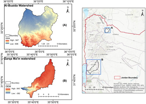
The mean annual rainfalls calculated in the stations Madaba, Ma’in, and Mushaqqar are 319, 264, and 333 mm, respectively. Winter-growing crops and rangeland cover 67.861% of the watershed land use and land cover, of which 30.245% is crops and 37.616% is rangeland. Built area, bare ground, and roads comprised 17.28%, 9.5%, and 5.37%, respectively.

However, the Al-Buaida Watershed (longitude 36°01′15″ to 36°08′15″ and latitude 32°22′45″ to 32°28′10″) is a small one located in the north of Jordan (Figure 1). The watershed covers an area of approximately 71.24 km². The elevation varies between 667 and 947 m above mean sea level. Contrary to the Zarqa Ma’in watershed, the land has gentle to moderate slopes (0° and 24.72°). The watershed hydrologic soil groups are C and D, which characterize a soil containing silty clay loam, clay loam, sandy clay, clay, sandy clay loam, or silty clay.

The mean annual rainfall calculated for two stations (Khanasira and Hosha) is 188.6 and 142.5 mm, respectively. The rangeland comprises 70.8% of the land use and land cover, followed by bare land (19.2%), built areas (8.2%), roads (1.6%), and crops (0.2%) only.

3. Methodology

The study methodology comprised of two stages (Figure 2). The first stage is the generation of flood data by hydrologic modeling, whereas the second stage is the application of machine learning algorithms (MLAs) on the flood-generated data in the first stage.

Figure 2. Flowchart of the applied methodology.

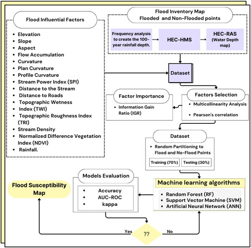
In the first stage, the daily observed rainfall data were used to generate the corresponding 100-year direct runoff and mark the flood and non-flood points in the watershed. The 100-year is used in flood studies in many parts of the world and incorporated in guidelines because it is a tradeoff between the level of protecting of structures and the cost incurred for protection. The HEC-HMS was used for runoff hydrograph generation and the HEC-RAS model for stream flow depth. Of the flooded and non-flooded marked points, 10,000 were randomly selected for the MLAs. Fifteen factors were initially considered influential for training and were later reduced to 13 after multicollinearity, and Pearson’s correlation analyses dropped two of them. Subsequently, 70% of flooded and non-flooded points were utilized for the training process, and the remaining were used for testing. Based on the results, a flood susceptibility map was generated. Details of these methods and their applications are described below.

3.1. Preprocessing and dataset preparation

3.1.1. Flood depth and velocity along the stream network

For generating the flood data from the hydrologic model, Zarqa Ma’in and Al-Buaida watersheds were first delineated from a 12.5 m resolution digital elevation model (DEM). To generate a 100-year flood hydrograph of the watershed, the annual series of maximum daily rainfall was extracted for each rainfall station, then subjected to a frequency analysis and fitted to these probability density functions: Normal, Log-Normal, Log-Pearson type III, and Gumbel.

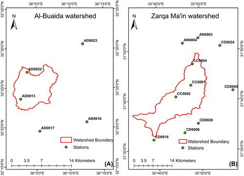
In Zarqa Ma’in watershed, data from ten rainfall stations was used, while in the Al-Buaida watershed, data from five stations was used (Figure 3). The analysis results are presented in Figures S1 and S2. Table S1 also provides a summary of the values for all stations along with the predicted 100-year maximum daily rainfalls.

Figure 3. Rainfall station location.

The Natural Resources Conservation Service-Curve Number (NRCS-CN) method and the Soil Conservation Service (SCS) lag-time method, embedded in HEC-HMS, were employed to generate the direct runoff hydrograph. In the application, it was assumed that rainfall temporal distribution is Type II, rainfall duration is 24-h, and antecedent soil moisture conditions are No. II. For the spatial distribution of rainfall over the watershed, the inverse distance weighting (IDW) method was used.

For flow depth and velocity along the stream network, the hydraulic model HEC-RAS was used. The rain-on-grid discretization was adopted because it accommodates spatial rainfall and infiltration distribution reasonably (Costabile et al. 2021). The model outputs are flow depth and velocity at several locations along the streams.

3.1.2. Flood inventory map

Flood locations as points play an essential role in understanding the correlation between flood occurrences and the underlying flood-influential factors (Darabi et al. 2019). These points form the basis of flood inventory maps, or maps of past events, which are key for predicting future flood incidents. The fundamental concept underlying flood points is that expected floods are likely to exhibit similar circumstances to past floods (Avand et al. 2021).

Prior research has mainly utilized a limited number of flood points, along with flood inventory maps sourced from field surveys or historical flood records. Recorded flood-inundation data often lacks precise spatial information and is frequently outdated. In addition, sparsely distributed points lead to a shortage in the training process of machine-learning algorithms. This leads to limitations in predicting the flood likelihood (Chen et al. 2021). Therefore, the existence of a comprehensive and unbiased flood dataset is essential because it offers continuous spatial coverage and incorporates the details of all influential factors. This dataset functions as the basis for the robust training and validation processes (Fang et al. 2022). In this study, the flood depth maps generated from the HEC-RAS model were converted into a points-based format. Points with insignificant flood depths were excluded. Moreover, using ArcGIS, a random sampling method was used to select 5000 points from areas with high flood depths and velocities, ensuring that the sampled flood points representing severe flooding conditions, or what is called a watershed inventory map (Figures 4 and 5).

Figure 4. Zarqa Ma’in watershed DEM and the 100-year flooding depth.

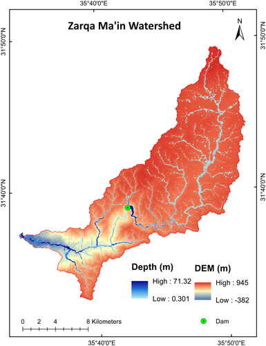
Figure 5. Al-Buaida watershed DEM and the 100-year flooding depth.

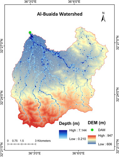
For the non-flooded points, we used random sampling to select 5000 points from areas with no flood depth, with a focus on high-elevation areas, such as mountains and hills, where floods rarely occur. This approach provided a balanced dataset of flood and non-flood points. Similar to previous studies, where data was randomly split, 70% was allocated for model training and 30% was allocated for model testing (Fang et al. 2022; Saikh and Mondal 2023; Li and Hong 2023).

3.1.3. Flood influential factors

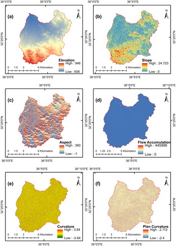
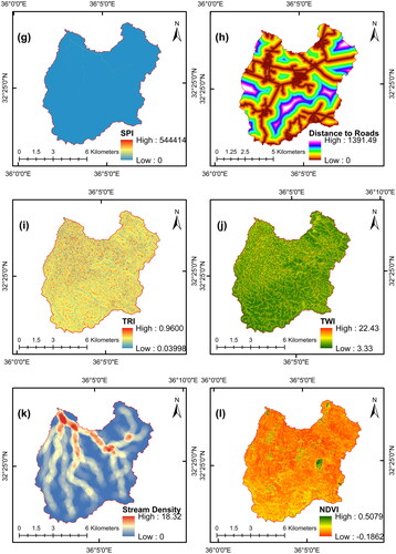
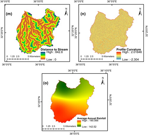
Factors that contribute to flooding are essential for any study that aims to create an accurate flood model for predicting the likelihood of floods. The significance of these factors varies from one case study to another (Kia et al. 2012). However, the selection of these factors was based on the specific characteristics of the case study, the availability of data, and knowledge obtained from the literature (Hasanuzzaman et al. 2022). Table S2 summarizes the factors used in various studies. In our case studies, we considered 15 factors based on data availability and the literature. Most factors were derived from digital elevation models (DEMs) with 12.5-meter resolution from the Alaska Satellite Facility (ALOS PALSAR), including elevation, slope, aspect, flow accumulation, land curvature, profile curvature, plan curvature, stream power index (SPI), distance to the stream, topographic wetness index (TWI), topographic roughness index (TRI), and stream density. The road map was obtained from OpenStreetMap (https://www.openstreetmap.org/) in vector map, and the NDVI factor was derived using multispectral images from Sentinel-2, a satellite-based remote sensing system. The spatial distribution of them for both watersheds is presented in Figures 6 and 7. ArcGIS version 10.3 was used to generate all the factors used in the raster format. The following is a description of the 15 factors considered.

Figure 6. Selected flood influential factors for Zarqa Ma’in watershed.

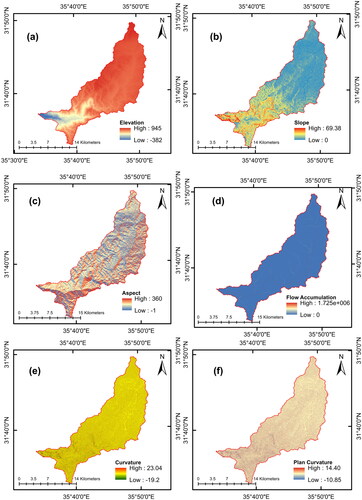
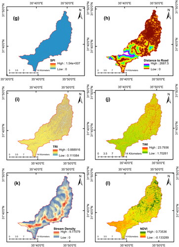
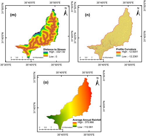
Figure 7. Selected flood influential factors for Al-Buaida watershed.

• Elevation

  Elevation affects the speed and direction of surface runoff, making it a crucial factor in flooding dynamics (Avand et al. 2021). Areas with lower elevations are more prone to flooding than those in high areas (Farhadi and Najafzadeh 2021).

• Slope

  Slope is one of the main factors affecting flooding; it causes water to flow downslope at faster rates, allowing for less infiltration (Edamo et al. 2022). Lowlands, or flatlands, that are characterized by gentle slopes pose a constant flood hazard (Wang et al. 2015; Darabi et al. 2019).

• Aspect

  Aspect is the direction of the steepest slope on the earth’s surface (Youssef et al. 2022). It ranges from 0 to 360°, measured clockwise from the north, and cells with flat areas are assigned an aspect equal to −1 (Edamo et al. 2022).

• Flow accumulation

  Flow accumulation determines where the flow can accumulate over the watershed to form the stream network. It is important for predicting the potential for flooding (Edamo et al. 2022).

• Distance to streams

  The distance to the stream influences the likelihood of flooding. The further away from streams, the lower the likelihood of flooding (Khosravi et al. 2018; Hasanuzzaman et al. 2022).

• Curvature

  Curvature, either flat, concave, or convex, determines the rate of change in the slope inclination at a specific point on a surface. This significantly affects surface runoff and infiltration (Chapi et al. 2017; Youssef et al. 2022). However, there are two common forms of curvature: plan and profile (Youssef et al. 2022). The profile curvature is the rate of change of the slope that aligns with the steepest slope direction. The plan curvature is perpendicular to the direction of the steepest slope (Deroliya et al. 2022).

• Stream Power Index (SPI)

  The Stream Power Index (SPI) is a geomorphic index describing the erosive potential of water flow within watersheds. SPI, as defined in Equation (1)(1) $$\mathrm{\text{SPI}}={\mathrm{A}}_{\mathrm{s}}\mathrm{\text{tan}}\hspace{0.17em}\text{β}$$(1) , illustrates the erosive power of overland flow and its influence on flooding likelihood (Khosravi et al. 2018; Youssef et al. 2022). (1) $$\mathrm{\text{SPI}}={\mathrm{A}}_{\mathrm{s}}\mathrm{\text{tan}}\hspace{0.17em}\text{β}$$(1)

  Where ${\mathrm{A}}_{\mathrm{s}}$ is the watershed area and $\mathrm{\beta }$ is the slope angle (degrees).

• Distance to roads.

  Distance to roads is an indicator of highly impervious surfaces that amplify flooding (Marco et al. 2022), which affects surface runoff and infiltration capacity (Nguyen 2022).

• Topographic Roughness Index (TRI)

  The topographic roughness index (TRI), as defined in Equation (2)(2) $$\mathrm{\text{TRI}}=\frac{\left({\mathrm{\text{FS}}}_{\mathrm{\text{mean}}}-{\mathrm{\text{FS}}}_{\mathrm{\text{min}}}\right)}{\left({\mathrm{\text{FS}}}_{\mathrm{\text{max}}}-{\mathrm{\text{FS}}}_{\mathrm{\text{min}}}\right)}$$(2) , detects how local basin topography impacts flooding, with lower values suggesting a greater flooding likelihood. (2) $$\mathrm{\text{TRI}}=\frac{\left({\mathrm{\text{FS}}}_{\mathrm{\text{mean}}}-{\mathrm{\text{FS}}}_{\mathrm{\text{min}}}\right)}{\left({\mathrm{\text{FS}}}_{\mathrm{\text{max}}}-{\mathrm{\text{FS}}}_{\mathrm{\text{min}}}\right)}$$(2)

  where ${\mathrm{\text{FS}}}_{\mathrm{\text{mean}}},$ ${\mathrm{\text{FS}}}_{\mathrm{\text{max}}}$ and ${\mathrm{\text{FS}}}_{\mathrm{\text{min}}}$ are the mean, maximum, and minimum values, respectively, within the focal statistical layers.

• Topographic Wetness Index (TWI)

  Topographic Wetness Index (TWI) describes the spatial distribution of elements such as soil moisture, water table depth, and soil wetness. TWI (Equation (3)(3) $$\mathrm{\text{TWI}}=\mathrm{\text{ln}}\left(\frac{\mathrm{\alpha }}{\mathrm{\text{tan}}\hspace{0.17em}\text{β}}\right)$$(3) ) measures the degree of wetness at a specific location by considering both the slope and area contributing to the upslope flow (Seleem et al. 2021; Plataridis and Mallios 2023). Higher TWI values in a region make it more susceptible to water accumulation, which increases the likelihood of flooding (Hasanuzzaman et al. 2022). (3) $$\mathrm{\text{TWI}}=\mathrm{\text{ln}}\left(\frac{\mathrm{\alpha }}{\mathrm{\text{tan}}\hspace{0.17em}\text{β}}\right)$$(3)

  where $\mathrm{\alpha }$ is the contributing upslope drainage area through the point, and $\mathrm{\text{tan}}\hspace{0.17em}\text{β}$ is the angle of slope at the point.

• Normalized Difference Vegetation Index (NDVI)

  Flooding is less likely to occur when vegetation covers the surface (Askar et al. 2022). NDVI is a measure of the amount of green vegetation in the watershed. In this study, images from Sentinel-2 were used to calculate NDVI using Equation (4)(4) $$\mathrm{\text{NDVI}}=\frac{\left(\mathrm{\text{NIR}}-\mathrm{R}\right)}{\left(\mathrm{\text{NIR}}+\mathrm{R}\right)}$$(4) (Farhadi and Najafzadeh 2021; Mahdizadeh Gharakhanlou and Perez 2023). (4) $$\mathrm{\text{NDVI}}=\frac{\left(\mathrm{\text{NIR}}-\mathrm{R}\right)}{\left(\mathrm{\text{NIR}}+\mathrm{R}\right)}$$(4)

  where NIR is the near infrared (band number eight in Sentinel-2 images), and R is the red band (band number four in Sentinel-2 images).

• Rainfall

  Rainfall is a crucial flood-influencing factor. In this study, it was obtained from the Ministry of Water and Irrigation (MWI).

• Stream density

  Stream density is a key flood-influential factor that affects flooding in watersheds. Regions with a high stream density exhibit a quick response, which increases the likelihood of flooding (Chapi et al. 2017).

3.2. Factors screening

3.2.1. Factor selection process

Prior to feeding data into MLAs, noisy data needs to be removed to enhance the accuracy and interpretability of the models. In our case studies, two methods were used to screen the factors importance: multicollinearity analysis and Pearson’s correlation.

Multicollinearity occurs when there is a high correlation between independent variables in a regression model. Therefore, it is crucial that researchers identify and remove them (Mansfield and Helms 1982). Multicollinearity can adversely affect the reliability of modeling outcomes (Mansfield and Helms 1982).

As some of the factors used in the model are generated from one input, such as DEM, multicollinearity is expected between the flood-influencing factors (Deroliya et al. 2022). Multicollinearity analysis in the Statistical Package for the Social Sciences (SPSS) was utilized to evaluate correlations among the factors. The variance inflation factor (VIF) is used to evaluate the strength of the correlations between the flood-influential factors (predictors). A VIF (Equation (5)(5) $${\mathrm{\text{VIF}}}_{\mathrm{I}}=\frac{1}{1-{\mathrm{R}}_{\mathrm{i}}^2}$$(5) ) value exceeding five is typically considered indicative of significant multicollinearity (Youssef et al. 2022). A regression model using ordinary least squares was developed. One factor served as a dependent factor, and the remaining factors served as independent factors. This process was repeated, and the R-squared value was calculated for each model (Youssef et al. 2022). (5) $${\mathrm{\text{VIF}}}_{\mathrm{I}}=\frac{1}{1-{\mathrm{R}}_{\mathrm{i}}^2}$$(5)

Pearson’s correlation was used to generate a correlation matrix that assesses the relationship between flood-influential factors (independent variables). This quantifies the strength of the relationships between each pair of factors. The value of Pearson’s coefficient ranged between −1 and +1. A value close to zero indicated that there was no relationship between the factors. If the value is close to +1, it indicates a strong positive relationship; if it is close to −1, it indicates a strong negative relationship (Al-Juaidi et al. 2018). Pearson’s correlation analysis was performed too, using Python with the Pandas, Matplotlib, and Seaborn libraries to measure the linear relationship among the factors. The combination of these two methods was aimed at ensuring a comprehensive evaluation of the selected factors and removing redundant ones.

The final set of factors, free from significant multicollinearity and featuring limited inter-variable correlation, was then utilized as inputs for the MLAs. This dual approach of two evaluation methods enhances the robustness of the factor selection process.

3.2.2. Factor importance evaluation

Information Gain Ratio (IGR) is a method used to assess the importance of input factors in MLAs, particularly in flood studies. It is employed to identify the most suitable factors with effective predictive capabilities (Plataridis and Mallios 2023). It is probable that some influencing factors lack predictive significance, whereas others introduce noise. Therefore, it is important to evaluate the impact of the selected factors. Using the IGR to assess the importance of these factors, its scores provide predictive strength, as a higher IGR value indicates greater predictive capability within the model (Chapi et al. 2017). Equations (6)–(9) are used to calculate the IGR scores for each factor selected in the models (Chapi et al. 2017; Khosravi et al. 2018). The process involved utilizing the scikit-learn library in Python to calculate the mutual information scores between each feature and target variable. (6) $$\mathrm{\text{IGR}}\left(\mathrm{D},\mathrm{f}\right)=\frac{\mathrm{\text{Entropy}}\mathrm{ }\left(\mathrm{D}\right)-\mathrm{\text{Entropy}}\mathrm{ }\left(\mathrm{D},\mathrm{f}\right)}{\mathrm{\text{SplitEntropy}}\mathrm{ }\left(\mathrm{D},\mathrm{f}\right)}$$(6) (7) $$\mathrm{\text{Entropy}}\left(D\right)=-\sum _{\mathrm{i}=1}^2\frac{\left({\mathrm{Y}}_{\mathrm{i}},\mathrm{f}\right)}{\left|\mathrm{D}\right|}{\mathrm{\text{log}}}_2\frac{\mathrm{n}\left({\mathrm{Y}}_{\mathrm{i}},\mathrm{f}\right)}{\left|\mathrm{D}\right|}$$(7) (8) $$\mathrm{\text{Entropy}}\left(\mathrm{D},\mathrm{f}\right)=-\sum _{\mathrm{j}=1}^{\mathrm{m}}\frac{{\mathrm{D}}_{\mathrm{j}}}{\left|\mathrm{D}\right|}\mathrm{\text{Entropy}}\left(\mathrm{D}\right)$$(8) (9) $$\mathrm{\text{SplitEntropy}}\mathrm{ }\left(\mathrm{D},\mathrm{f}\right)=-\sum _{\mathrm{j}=1}^{\mathrm{m}}\frac{\left|{\mathrm{D}}_{\mathrm{j}}\right|}{\left|\mathrm{D}\right|}{\mathrm{\text{log}}}_2\frac{\left|{\mathrm{D}}_{\mathrm{j}}\right|}{\left|\mathrm{D}\right|}$$(9)

Where D is a training dataset that contains (n) input samples, and $\mathrm{n}\left({\mathrm{Y}}_{\mathrm{i}},\mathrm{D}\right)$ represents the number of samples in the training dataset D that fall into the class label ${\mathrm{Y}}_{\mathrm{i}}$ (either Flood or Non-Flood). For instance, $\mathrm{n}\left({\mathrm{Y}}_{\mathrm{i}},{\mathrm{f}}_1\right)$ is the number of classes with the class label ${\mathrm{Y}}_{\mathrm{i}}$ (either Flood or Non-Flood) for factor ${\mathrm{f}}_1.$

3.3. Machine learning algorithms

3.3.1. Random forest

Random Forest (RF) is an ensemble machine learning algorithm that is widely recognized and commonly used for supervised learning tasks and in the application of flood susceptibility mapping (Hasanuzzaman et al. 2022; Seleem et al. 2022). It applies the bootstrap technique to generate new sub-data from the original data, with each sub-data having the same size as the original data (Wang et al. 2015; Youssef et al. 2022). For more details and a comprehensive explanation regarding the RF algorithm, readers can refer to Breiman (2001) and Wang et al. (2015). The training and testing dataset was used to train the Random Forest classifier from the scikit-learn library by employing a specific set of hyperparameters such as the number of estimators, maximum depth, and minimum samples per leaf. The validation techniques of k-fold cross-validation are used to tune the parameters. Table S3 presents the optimal hyperparameter values used.

3.3.2. Support vector machine

Support vector machine (SVM) is widely used in supervised MLAs for linearly separable binary datasets and is commonly utilized in the prediction of flooding likelihood (Tehrany et al. 2014; Youssef et al. 2022). SVM aims to find the decision boundaries and hyperplane that provide the maximum margin to separate datasets into two distinct classes, which enhances robustness and minimizes the chances of misclassification (Pradhan 2012). The SVM classifier from the scikit-learn library was used for flood prediction. A grid search with cross-validation was conducted using the ‘GridSearchCV' function from scikit-learn to explore hyperparameter combinations, including the cost parameter (C) and the radial basis function kernel parameter (gamma) (Mehravar et al. 2023) The optimal hyperparameter values are presented in Table S3. More insights regarding SVM are described in depth by Cortes and Vapnik (1995).

3.3.3. Artificial neural networks

Artificial neural networks (ANNs) are one of the primary MLAs and are a basic representation of brain-like systems that are frequently used in scientific research to address a variety of problems (problems (Kia et al. 2012; Mahdizadeh Gharakhanlou and Perez 2023). ANNs are among the primary MLAs used as powerful tools for flood likelihood prediction (Seleem et al. 2022). The fundamental architecture of this system comprises three essential layers: an input layer, single or multiple hidden layers, and an output layer (Marco et al. 2022). ANNs from the TensorFlow and Keras libraries were used. The model included connected layers with a rectified linear unit (ReLU) activation function, which was used to add nonlinearity. In addition, the sigmoid activation function was utilized for the output layer, which allowed for the interpretation of the output as a probability and prediction for the first and second classes (Kia et al. 2012; Seleem et al. 2022). During training, the goal is to determine the best connection weights by minimizing the cost function (Bishop 1995). Thus, the binary cross-entropy loss function and Adam optimizer were used. Moreover, a grid search was used to tune the hyperparameters, including batch size and learning rate. The optimal values are listed in Table S3. For more details regarding neural network algorithms, Bishop (1995) provides a deeper and more comprehensive explanation of the intricacies of neural networks.

3.4. Model performance evaluation

Three evaluation metrics were employed in this study: kappa, accuracy, and area under the relative operating characteristic curve (AUC-ROC). These metrics are among the most widely used methods in flood prediction research to evaluate the performance of MLAs (Plataridis and Mallios 2023). Among the RF, SVM, and ANN models, the one that showed the best performance was chosen to be used on the entire dataset of the case studies to generate the flood susceptibility map.

The AUC-ROC is a graphical representation that reflects the likelihood that the machine learning models can correctly categorize the points into flooded or non-flooded points. It is a plot of the sensitivity (Equation (10)(10) $$\mathrm{\text{Recall}}=\mathrm{\text{Sensitivity}}=\frac{\mathrm{\text{TP}}}{\mathrm{\text{TP}}+\mathrm{\text{FN}}}$$(10) ) (or true positive rate, TPR) on the y-axis and the 1-specificity (false positive rate, FPR) on the x-axis. The specificity (Equation (11)(11) $$\mathrm{\text{Specificity}}=\frac{\mathrm{\text{TN}}}{\mathrm{\text{TN}}+\mathrm{\text{FP}}}$$(11) ) is the true negative rate correctly predicted by the model (Deroliya et al. 2022; Mahdizadeh Gharakhanlou and Perez 2023). The AUC-ROC ranges from 0 to 1, where one indicates that the model prediction is ideal (Khosravi et al. 2018). Cohen’s kappa (k) is calculated using the following Equation (12)(12) $$\mathrm{k}=\frac{{\mathrm{P}}_{\mathrm{o}}-{\mathrm{P}}_{\mathrm{e}}}{1-{\mathrm{P}}_{\mathrm{e}}}$$(12) , and it measures the degree of consistency between the values predicted by machine learning models and the actual values. When the value of k is close to 1, it is close to agreement (Deroliya et al. 2022). (10) $$\mathrm{\text{Recall}}=\mathrm{\text{Sensitivity}}=\frac{\mathrm{\text{TP}}}{\mathrm{\text{TP}}+\mathrm{\text{FN}}}$$(10) (11) $$\mathrm{\text{Specificity}}=\frac{\mathrm{\text{TN}}}{\mathrm{\text{TN}}+\mathrm{\text{FP}}}$$(11) (12) $$\mathrm{k}=\frac{{\mathrm{P}}_{\mathrm{o}}-{\mathrm{P}}_{\mathrm{e}}}{1-{\mathrm{P}}_{\mathrm{e}}}$$(12) (13) $$P_o=\frac{\mathit{\text{TP}}+\mathit{\text{TN}}}{\mathit{\text{TP}}+\mathit{\text{TN}}+\mathit{\text{FN}}+\mathit{\text{FP}}}$$(13) (14) $$P_e=\frac{\left(\mathit{\text{TP}}+\mathit{\text{FN}}\right)\left(\mathit{\text{TP}}+\mathit{\text{FP}}\right)+\left(\mathit{\text{FP}}+\mathit{\text{TN}}\right)\left(\mathit{\text{FN}}+\mathit{\text{TN}}\right)}{{\left(\mathit{\text{TP}}+\mathit{\text{TN}}+\mathit{\text{FP}}+\mathit{\text{FN}}\right)}^2}$$(14)

Where TP is the true positive, TN is the true negative, FP is the false positive, and FN is the false negative rate. Po is the percentage of the observed agreement between the machine learning model and the actual values, and Pe is the percentage of such an agreement predicted by chance.

Additionally, accuracy, which is the ratio of correctly predicted flooded or non-flooded points to the total number of points used as model inputs, is another statistical measure used to assess the effectiveness of MLAs and is calculated using equation (Li et al. 2021; Saber et al. 2023). It also ranges from 0 to 1, with 1 indicating perfect accuracy. (15) $$\mathrm{\text{Accuracy}}=\frac{\mathrm{\text{TP}}+\mathrm{\text{TN}}}{\mathrm{\text{TP}}+\mathrm{\text{TN}}+\mathrm{\text{FP}}+\mathrm{\text{FN}}}$$(15)

4. Results and discussion

4.1. Factors selection

Both Zarqa Ma’in and Al-Buaida watersheds met the threshold value of five for all factors except curvature, plan curvature, and profile curvature, which seemed to be correlated with other variables (Table 1). This issue is expected because plan curvature and profile curvature are the predominant forms of curvature. Therefore, the plan and profile curvatures were removed. Consequently, the VIF value after removing them settled at less than five. This removal is necessary for the reliability and interpretability of the models.

Table 1. VIF values in multicollinearity analysis for all flood influential factors.

	Factor	VIF
		Zarq Ma’in	Al-Buaida
1	Elevation	4.33	4.998
2	Slope	2.028	2.062
3	Aspect	1.217	1.07
4	Flow accumulation	3.209	4.421
5	Curvature	50.124*	42.91**
6	Plan curvature	15.61	13.538
7	Profile curvature	19.493	15.88
8	SPI	2.042	4.265
9	Distance to stream	1.661	1.992
10	Distance to roads	1.247	1.065
11	TRI	2.094	1.292
12	TWI	3.259	2.437
13	NDVI	4.509	2.975
14	Stream density	1.66	2.069
15	Average annual rainfall	4.537	4.685

The value marked with (*) becomes 3.21 after excluding profile and plan curvature. The value marked with (**) becomes 2.42.

Pearson’s correlation was also used to assess the correlation between flood-influential factors. As illustrated in Figures S2 and S3, curvature demonstrated a robust positive correlation with plan curvature and a substantial negative correlation with profile curvature, indicating that these variables were highly associated with each other. The set of factors, free from significant multicollinearity and characterized by minimal inter-variable correlation, were then employed as input features for the machine learning classification models. This dual-method approach reduces the 15 influential factors to 13.

4.2. Features importance

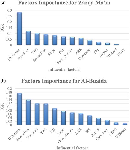
IGR was utilized for identifying the importance of flood-influential factors, and the outcomes are presented in Figure 8. In Zarqa Ma’in watershed, the distance to stream is the most important factor; it has a high IGR of 28.31%. However, the distance to stream, elevation, and TWI combined have almost 50% IGR value, underscoring their pivotal role in improving the model’s ability to recognize and predict patterns. In contrast, Aspect, SPI, distance to road, and NDVI have comparatively low IGR values (5%), suggesting a lack of predictability power during the model training process. In Al-Buaida watershed, distance to stream, like in Zarqa Ma’in watershed, is the most influential factor with an IGR of 17.47%, followed by stream density with a 14% IGR. The factors with the least predictive power are distance to the road, NDVI, curvature, and aspect, with a combined IGR of almost 9%.

Figure 8. Importance sequence of flood influential factors for (a) Zarqa Ma’in watershed and (b) Al-Buaida watershed. Where DTStream is the distance to the stream, StreamDen is the stream density, flow_accum is the flow accumulation, AAR is the average annual rainfall, and DTRoad is the distance to the roads.

Moreover, irrespective of the order, the first six most important factors in both watersheds are the same. These results are in line with those found in the literature (Farhadi and Najafzadeh 2021; Abu El-Magd et al. 2022; Askar et al. 2022). Nevertheless, the distance to stream is the most significant factor here, similar to other literature sources (Darabi et al. 2019; Abu El-Magd et al. 2022; Sachdeva and Kumar 2022; Taromideh et al. 2022; Mehravar et al. 2023). This emphasizes the significance of this factor in flood management and flooding likelihood.

4.3. Models’ evaluation and performance

Assessing MLAs’ performance on training and testing datasets of Zarqa Ma’in and Al-Buaida watersheds provides valuable perspectives on their effectiveness for predicting flood-prone areas. The three algorithms were assessed based on three key metrics: kappa, area AUC-ROC, and accuracy. The results for the training and testing datasets are presented in Table 2. Figures 9 and 10 show the AUC-ROC for both watersheds for training datasets. This assessment illustrates that all algorithms demonstrated excellent performance in both watersheds.

Figure 9. The AUC-ROC curve for Zarqa Ma’in watershed for the training dataset.

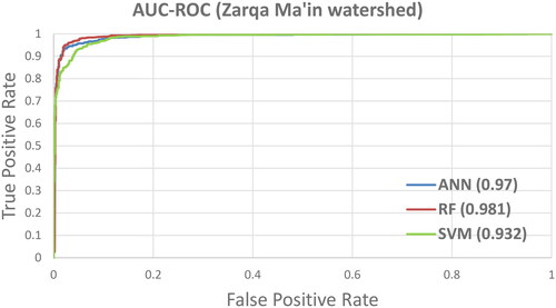
Figure 10. The AUC-ROC curve for Al-Buaida watershed for the training dataset.

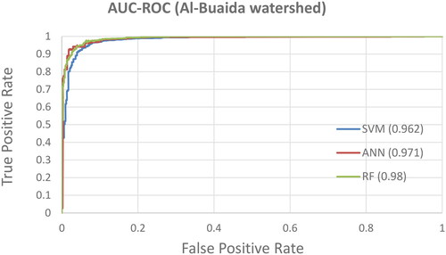
Table 2. Models’ performance using training and testing datasets for Zarqa Ma’in and Al-Buaida watersheds.

	Zarqa Ma’in			Al-Buaida
	Training Dataset
Model name	kappa	AUC-ROC	Accuracy	kappa	AUC-ROC	Accuracy
Random forest (RF)	0.931	0.981	0.972	0.92	0.98	0.974
Support vector machine (SVM)	0.865	0.9321	0.933	0.876	0.962	0.942
Artificial neural network (ANN)	0.903	0.971	0.951	0.864	0.971	0.936
	Testing Dataset
Random forest (RF)	0.928	0.98	0.964	0.901	0.98	0.9517
Support vector machine (SVM)	0.85	0.931	0.928	0.857	0.951	0.934
Artificial neural network (ANN)	0.891	0.966	0.942	0.855	0.97	0.932

The comparative evaluation among the three models illustrates that the RF model outperforms the SVM and ANN in terms of key metrics. In the training dataset, RF exhibited robust performance in both Zarqa Ma’in and Al-Buaida watersheds, achieving high kappa values of 0.93 and 0.92, AUC-ROC scores of 0.981 and 0.98, and high accuracy of 0.972 and 0.974, respectively, in both watersheds. While in the testing dataset, RF maintains its solid performance, with high kappa values (0.928 and 0.901), AUC-ROC scores (0.98 and 0.98), and accuracy (0.964 and 0.9517) for Zarqa Ma’in and Al-Buaida watersheds, respectively. This suggests that the RF could be a robust choice for predicting flood-prone areas. However, the performances of SVM and ANN remain efficacious and significant. Multiple studies have agreed that RF is the top-performing model. In a study by Hasanuzzaman et al. (2022), which compared RF, Naive Bayes (NB), and Extreme Gradient Boosting (XGB), RF exhibited superior performance. Similarly, Youssef et al. (2022) found that RF outperformed seven other models.

4.4. Generating flood susceptibility maps

The creation of a precise flood susceptibility map is essential for making effective and productive strategies to mitigate the impact of flood-related damage. Prior investigations on flood susceptibility mapping worldwide have employed machine learning methods and deep learning. Therefore, extensive model testing is highly recommended, particularly in regions with limited data. In our study, we used three models: RF, SVM, and ANN. All three algorithms demonstrated excellent performance, with an outperformance for the RF algorithm in both case studies, and it is used to generate the flood susceptibility map. The process involved incorporating the entire case study area as points, with values matching the factors used in the training stage, transforming the resultant flood susceptibility predictions into raster maps, and subsequently classifying them into five categories using the natural break method.

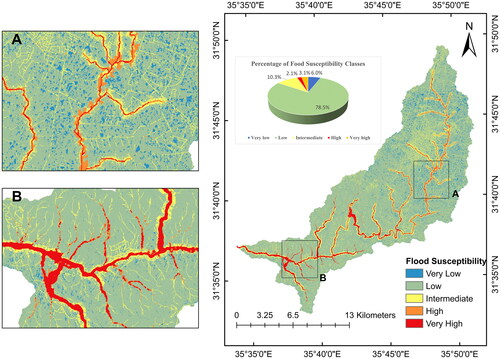
The resulting flood susceptibility map for the Zarqa Ma’in Watershed revealed distinct spatial patterns (Figure 11). Most of the area falls into the ‘low’ susceptibility class, constituting 78.5%. This indicates that a significant portion of the region has a low risk of flooding. Conversely, the ‘Very Low’ susceptibility class covered 6.0% of the study area, indicating areas with a moderate level of vulnerability. The ‘high’ and ‘very high’ susceptibility classes make up smaller percentages, reflecting localized areas with elevated flood risk. However, most of the areas with high and very high susceptibility classes are located in and near wadies. Our models support previous research, which shows that lower-elevation locations near riverbanks and stream drainage systems are more vulnerable to flooding (Bui et al. 2019; Seleem et al. 2022).

Figure 11. Flood susceptibility map for Zarqa Ma’in watershed.

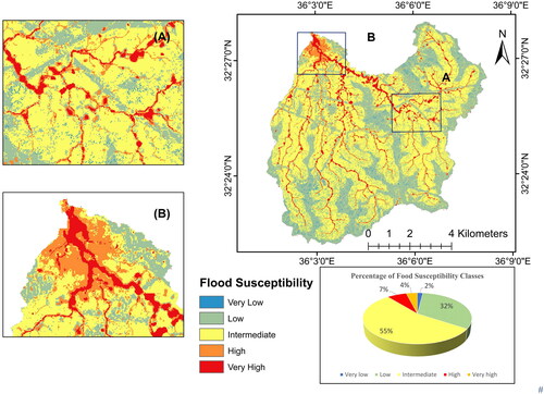
The flood susceptibility map of the Al-Buaida watershed shows a different distribution (Figure 12). Most of the region falls within the ‘intermediate’ susceptibility class, which comprises 55% of the total area. This suggests that a significant portion of the study area has a moderate level of susceptibility to flooding. The ‘low’ susceptibility class covers 32%, indicating areas with a relatively lower risk. The ‘high’ susceptibility class represents 7%, indicating specific regions with greater vulnerability. Additionally, the ‘Very Low’ and ‘Very High’ susceptibility classes each contribute 2% and 4%, respectively, depicting areas with the lowest and highest flood susceptibility.

Figure 12. Flood susceptibility map for Al-Buaida watershed.

4.5. Effectiveness of the model hybrid approach

The hybrid approach between hydrodynamic methods (HDM) and MLAs in the creation of flood susceptibility maps represents a highly effective approach, especially when compared to conventional methods that depend only on public records or governmental datasets. Because of the accuracy and continuous nature of hydrodynamic simulation results, this study adopted a new perspective by converting the HDM outcomes into point data, which was subsequently used to train the three point-based classification models: RF, SVM, and ANN.

Prior research has mainly utilized a limited number of flood points, along with flood inventory maps sourced from field surveys or historical flood records. Recorded flood-inundation data often lacks precise spatial information and is outdated. In addition, sparsely distributed points lead to a shortage in the training process for MLAs. This leads to limitations in predicting the flood likelihood (Chen et al. 2021). One notable strength of this hybrid approach is the generation of a significantly larger dataset for training MLAs compared to conventional methods, which will improve their performance in predicting the likelihood of flooding.

The proposed methodology overcomes the limitations associated with historical flood records and field surveys by providing many data points relevant to MLA applications. Additionally, the effectiveness of this approach is demonstrated by the considerably high performance of the used accuracy, kappa, and AUC-ROC. This hybrid approach addresses the obstacles faced by data-scarce countries by addressing the limitations associated with sparse historical records. However, the effectiveness of this hybrid approach, substantial computational requirements, and extended processing duration within the suggested framework provide significant constraints that limit its widespread adoption.

5. Conclusion

Creating an accurate map of flooding likelihood can be beneficial for developing successful plans to minimize the effects of flood-related damage. The present study utilized MLAs to predict the flooding likelihood in two distinct watersheds: Zarqa Ma’in and Al-Buaida. The following is a summary of the research conclusions and findings:

• In this study, we explored the application of three MLAs in the prediction of flooding likelihood, demonstrating excellent performance in both case studies, with Random Forest slightly outperforming the other two.

• The hybrid between hydrodynamic models and MLAs, specifically the use of 100-year depth maps, has proven to be a successful step in enhancing the prediction abilities of the models by increasing the number of data points used in the training and testing processes. This is illustrated by the evaluation metrics results, as the accuracy, kappa, and AUC for the outperformed model were 0.972, 0.931, and 0.981, respectively, for Zarqa main watershed and 0.974, 0.92, and 0.98, respectively, for Al-Buaida watershed.

• Our findings illustrate the significance of low-lying areas near riverbanks and stream drainages as particularly susceptible to floods, aligning with existing literature. Additionally, areas surrounded by mountains, for instance, in the Zarqa Main watershed, were classified as highly susceptible. The distance to stream was the most important factor, with an IGR percentage of 28.31 in Zarqa Ma’in watershed and 17.473 in Al-Buaida watershed, illustrating its importance in flood susceptibility assessments, which aligns with previous research.

• Furthermore, the first six most important factors (slope, elevation, stream density, distance to stream, TWI, and TRI) in both watersheds, despite the slight variation in their order of importance, matched the existing literature. This study illustrated the distinct nature of predictive modeling, which shows the need for a detailed understanding of complex factor relationships.

• The hybrid approach, which facilitates the generation of a substantial volume of high-quality training data and results in robust predictive models, is a significant advantage of the proposed methodology. This framework, which is particularly useful for data-scarce countries where historical flood records are scarce, presents a promising process for advancing flood susceptibility mapping.

• This research provides valuable knowledge for planners, decision-makers, and other stakeholders, providing them with valuable perspectives through the generated flood susceptibility maps. These maps can serve as an essential step in any flood risk assessment study and as guides for establishing rules and regulations, such as mitigating urbanization in areas classified as highly susceptible to floods.

This study contributes to the field of flood susceptibility mapping and provides a useful solution that can guide adaptive decision-making and urban development plans. As recommendations for future research, it would be beneficial to extend the scope of flood susceptibility studies by incorporating various risk levels and moving farther than binary classifications. Additionally, future research exploring the concept of transfer learning could offer perspectives on the generalizability and flexibility of models across geographical and environmental settings. These recommendations will help provide knowledge for efficient flood risk management.

Acknowledgment

The authors would like to express their gratitude to Jordan University of Science and Technology for providing logistical assistance that contributed to the completion of this research.

Data availability statement

In this research, the data are available upon reasonable request from the corresponding author.

Disclosure statement

The authors declare that there are no conflicting interests regarding this study.

References

- Ababsa M, editor. 2013. Atlas of Jordan. In: Beyrouth: Presses de l’Ifpo. doi: 10.4000/books.ifpo.4560. Digital ISBN: 978-2-35159-438-4.
- Abdelal Q, Al-Rawabdeh A, Al Qudah K, Hamarneh C, Abu-Jaber N. 2021. Hydrological assessment and management implications for the ancient Nabataean flood control system in Petra, Jordan. J Hydrol. 601:126583. doi: 10.1016/j.jhydrol.2021.126583.
- Abu El-Magd SA, Maged A, Farhat HI. 2022. Hybrid-based Bayesian algorithm and hydrologic indices for flash flood vulnerability assessment in coastal regions: machine learning, risk prediction, and environmental impact. Environ Sci Pollut Res Int. 29(38):57345–57356. doi: 10.1007/s11356-022-19903-7.
- Abu Islaih A, Yaghan R, Al Kuisi M, Al-Bilbisi H. 2020. Impact of climate change on flash floods using hydrological modelling and GIS: case study Zarqa Ma’in area. Int J Appl Nat Sci (IJANS). 9:29–52.
- Al-Juaidi AEM, Nassar AM, Al-Juaidi OEM. 2018. Evaluation of flood susceptibility mapping using logistic regression and GIS conditioning factors. Arab J Geosci. 11(24):1–10. doi: 10.1007/s12517-018-4095-0.
- Al-Taani A, Al-Husban Y, Ayan A. 2023. Assessment of potential flash flood hazards. Concerning land use/land cover in Aqaba Governorate, Jordan, using a multi-criteria technique. Egypt J Remote Sens Space Sci. 26(1):17–24. doi: 10.1016/j.ejrs.2022.12.007.
- Askar S, Zeraat Peyma S, Yousef MM, Prodanova NA, Muda I, Elsahabi M, Hatamiafkoueieh J. 2022. Flood susceptibility mapping using remote sensing and integration of decision table classifier and metaheuristic algorithms. Water (Switzerland). 14(19):3062. doi: 10.3390/w14193062.
- Avand M, Moradi H, Lasboyee MR. 2021. Spatial modeling of flood probability using geo-environmental variables and machine learning models, case study: Tajan watershed, Iran. Adv Space Res. 67(10):3169–3186. doi: 10.1016/j.asr.2021.02.011.
- Bhattarai Y, Duwal S, Sharma S, Talchabhadel R. 2024. Leveraging machine learning and open-source spatial datasets to enhance flood susceptibility mapping in transboundary river basin. Int J Digit Earth. 17(1):1–24. doi: 10.1080/17538947.2024.2313857.
- Bishop CM. 1995. Neural networks for pattern recognition CLARENDON PRESS • OXFORD 1995.
- Breiman L. 2001. Random forests. Mach Learn. 45(1):5–32. doi: 10.1023/A:1010933404324.
- Bui DT, Khosravi K, Shahabi H, Daggupati P, Adamowski JF, Melesse M, Pham A, Pourghasemi BT, Mahmoudi HR, Bahrami M, et al. 2019. Flood spatial modeling in Northern Iran using remote sensing and GIS: a comparison between evidential belief functions and its ensemble with a multivariate logistic regression model. Remote Sens (Basel). 11(13):1589. doi: 10.3390/rs11131589.
- Chapi K, Singh VP, Shirzadi A, Shahabi H, Bui DT, Pham BT, Khosravi K. 2017. A novel hybrid artificial intelligence approach for flood susceptibility assessment. Environ Modell Software. 95:229–245. doi: 10.1016/j.envsoft.2017.06.012.
- Chen J, Huang G, Chen W. 2021. Towards better flood risk management: assessing flood risk and investigating the potential mechanism based on machine learning models. J Environ Manage. 293:112810. doi: 10.1016/j.jenvman.2021.112810.
- Chen J. 2023. Dynamic and loss analysis of flood inundation in the floodplain area of the lower Yellow River considering ecological impact. J Eng Appl Sci. 70(1):1–12. doi: 10.1186/s44147-023-00197-6.
- Cortes C, Vapnik V. 1995. Support-vector networks editor. Mach Learn. 20(3):273–297. doi: 10.1007/BF00994018.
- Costabile P, Costanzo C, Ferraro D, Barca P. 2021. Is HEC-RAS 2D accurate enough for storm-event hazard assessment? Lessons learnt from a benchmarking study based on rain-on-grid modelling. J Hydrol (Amst). 603:126962. doi: 10.1016/j.jhydrol.2021.126962.
- Darabi H, Choubin B, Rahmati O, Torabi Haghighi A, Pradhan B, Kløve B. 2019. Urban flood risk mapping using the GARP and QUEST models: a comparative study of machine learning techniques. J Hydrol (Amst). 569:142–154. doi: 10.1016/j.jhydrol.2018.12.002.
- Deroliya P, Ghosh M, Mohanty MP, Ghosh S, Rao KHVD, Karmakar S. 2022. A novel flood risk mapping approach with machine learning considering geomorphic and socio-economic vulnerability dimensions. Sci Total Environ. 851(Pt 1):158002. doi: 10.1016/j.scitotenv.2022.158002.
- Duwal S, Liu D, Pradhan PM. 2023. Flood susceptibility modeling of the Karnali river basin of Nepal using different machine learning approaches. Geomat Nat Hazards Risk. 14(1):1–25. doi: 10.1080/19475705.2023.2217321.
- Edamo ML, Ukumo TY, Lohani TK, Ayana MT, Ayele MA, Mada ZM, Abdi DM. 2022. A comparative assessment of multi-criteria decision-making analysis and machine learning methods for flood susceptibility mapping and socio-economic impacts on flood risk in Abela-Abaya floodplain of Ethiopia. Environ Challenges. 9:100629. doi: 10.1016/j.envc.2022.100629.
- Fang L, Huang J, Cai J, Nitivattananon V. 2022. Hybrid approach for flood susceptibility assessment in a flood-prone mountainous catchment in China. J Hydrol (Amst). 612:128091. doi: 10.1016/j.jhydrol.2022.128091.
- Farhadi H, Najafzadeh M. 2021. Flood risk mapping by remote sensing data and random forest technique. Water (Switzerland). 13(21):3115. doi: 10.3390/w13213115.
- Farhan Y, Ayed A. 2017. Assessment of flash-flood hazard in arid watersheds of Jordan. JGIS. 09(06):717–751. doi: 10.4236/jgis.2017.96045.
- Ferraro D, Costabile P, Costanzo C, Petaccia G, Macchione F. 2020. A spectral analysis approach for the a priori generation of computational grids in the 2-D hydrodynamic-based runoff simulations at a basin scale. J Hydrol (Amst). 582:124508. doi: 10.1016/j.jhydrol.2019.124508.
- Gudiyangada Nachappa T., Tavakkoli Piralilou, S., Gholamnia, K., Ghorbanzadeh, O., Rahmati, O., Blaschke, T., 2020. Flood susceptibility mapping with machine learning, multicriteria decision analysis and ensemble using Dempster Shafer Theory. J Hydrol (Amst). https://doi.org/10.1016/j.jhydrol.2020.125275.
- Hasanuzzaman M, Islam A, Bera B, Shit PK. 2022. A comparison of performance measures of three machine learning algorithms for flood susceptibility mapping of river Silabati (tropical river, India). Phys Chem Earth. 127:103198. doi: 10.1016/j.pce.2022.103198.
- Khosravi K, Pham BT, Chapi K, Shirzadi A, Shahabi H, Revhaug I, Prakash I, Tien Bui D. 2018. A comparative assessment of decision trees algorithms for flash flood susceptibility modeling at Haraz watershed, northern Iran. Sci Total Environ. 627:744–755. doi: 10.1016/j.scitotenv.2018.01.266.
- Kia MB, Pirasteh S, Pradhan B, Mahmud AR, Sulaiman WNA, Moradi A. 2012. An artificial neural network model for flood simulation using GIS: Johor River Basin, Malaysia. Environ Earth Sci. 67(1):251–264. doi: 10.1007/s12665-011-1504-z.
- Li Y, Hong H. 2023. Modelling flood susceptibility based on deep learning coupling with ensemble learning models. J Environ Manage. 325(Pt A):116450. doi: 10.1016/j.jenvman.2022.116450.
- Li Z, Liu H, Luo C, Fu G. 2021. Assessing surface water flood risks in urban areas using machine learning. Water (Switzerland). 13(24):3520. doi: 10.3390/w13243520.
- Liao M, Wen H, Yang L, Wang G, Xiang X, Liang X. 2024. Improving the model robustness of flood hazard mapping based on 2 hyperparameter optimization of random forest.
- Liu J, Wang J, Xiong J, Cheng W, Li Y, Cao Y, He Y, Duan Y, He W, Yang G. 2022. Assessment of flood susceptibility mapping using support vector machine, logistic regression and their ensemble techniques in the belt and road region. Geocarto Int. 37(25):9817–9846. doi: 10.1080/10106049.2022.2025918.
- Mahdizadeh Gharakhanlou N, Perez L. 2023. Flood susceptible prediction through the use of geospatial variables and machine learning methods. J Hydrol (Amst). 617:129121. doi: 10.1016/j.jhydrol.2023.129121.
- Mansfield ER, Helms BP. 1982. Detecting multicollinearity. Am Stat. 36(3a):158–160. doi: 10.1080/00031305.1982.10482818.
- Marco Z, Elena A, Anna S, Silvia T, Andrea C. 2022. Spatio-temporal cross-validation to predict pluvial flood events in the metropolitan city of Venice. J Hydrol (Amst). 612:128150. doi: 10.1016/j.jhydrol.2022.128150.
- Mehravar S, Razavi-Termeh SV, Moghimi A, Ranjgar B, Foroughnia F, Amani M. 2023. Flood susceptibility mapping using multi-temporal SAR imagery and novel integration of nature-inspired algorithms into support vector regression. J Hydrol (Amst). 617:129100. doi: 10.1016/j.jhydrol.2023.129100.
- Meliho M, Khattabi A, Driss Z, Orlando CA. 2022. Spatial prediction of flood-susceptible zones in the Ourika watershed of Morocco using machine learning algorithms. ACI. vol (ahed-of-print):1–13. doi: 10.1108/ACI-09-2021-0264.
- Mousavi SM, Ataie-Ashtiani B, Hosseini SM. 2022. Comparison of statistical and MCDM approaches for flood susceptibility mapping in northern Iran. J Hydrol (Amst). 612:128072. doi: 10.1016/j.jhydrol.2022.128072.
- Muhury N, Apan AA, Marasani TN, Ayele GT. 2022. Modelling floodplain vegetation response to groundwater variability using the ArcSWAT hydrological model, MODIS NDVI data, and machine learning. Land (Basel). 11(12):2154. doi: 10.3390/land11122154.
- Nguyen HD. 2022. GIS-based hybrid machine learning for flood susceptibility prediction in the Nhat Le–Kien Giang watershed, Vietnam. Earth Sci Inform. 15(4):2369–2386. doi: 10.1007/s12145-022-00825-4.
- Pham BT, Jaafari A, Phong TV, Yen HPH, Tuyen TT, Luong V, Van Nguyen HD, Le H, Foong LK. 2021a. Improved flood susceptibility mapping using a best first decision tree integrated with ensemble learning techniques. Geosci Front. 12(3):101105. doi: 10.1016/j.gsf.2020.11.003.
- Pham BT, Luu C, Phong TV, Nguyen HD, Le HV, Tran TQ, Ta HT, Prakash I. 2021b. Flood risk assessment using hybrid artificial intelligence models integrated with multi-criteria decision analysis in Quang Nam Province, Vietnam. J Hydrol (Amst). 592:125815. doi: 10.1016/j.jhydrol.2020.125815.
- Plataridis K, Mallios Z. 2023. Flood susceptibility mapping using hybrid models optimized with Artificial Bee Colony. J Hydrol (Amst). 624:129961. doi: 10.1016/j.jhydrol.2023.129961.
- Pradhan A. 2012. Support vector machine-a survey. Int J Emerg Tech Adv Eng. 2:82–85.
- Pradhan B, Lee S, Dikshit A, Kim H. 2023. Spatial flood susceptibility mapping using an explainable artificial intelligence (XAI) model. Geosci Front. 14(6):101625. doi: 10.1016/j.gsf.2023.101625.
- Razavi-Termeh SV, Sadeghi-Niaraki A, Seo MB, Choi SM. 2023. Application of genetic algorithm in optimization parallel ensemble-based machine learning algorithms to flood susceptibility mapping using radar satellite imagery. Sci Total Environ. 873:162285. doi: 10.1016/j.scitotenv.2023.162285.
- Saber M, Boulmaiz T, Guermoui M, Abdrabo KI, Kantoush SA, Sumi T, Boutaghane H, Hori T, Binh DV, Nguyen BQ, et al. 2023. Enhancing flood risk assessment through integration of ensemble learning approaches and physical-based hydrological modeling. Geomatics Nat Hazards Risk. 14(1):1–38. doi: 10.1080/19475705.2023.2203798.
- Sachdeva S, Kumar B. 2022. Flood susceptibility mapping using extremely randomized trees for Assam 2020 floods. Ecol Inform. 67:101498. doi: 10.1016/j.ecoinf.2021.101498.
- Saikh NI, Mondal P. 2023. GIS-based machine learning algorithm for flood susceptibility analysis in the Pagla river basin, Eastern India. Natural Hazards Res. 3(3):420–436. doi: 10.1016/j.nhres.2023.05.004.
- Seleem O, Ayzel G, de Souza ACT, Bronstert A, Heistermann M. 2022. Towards urban flood susceptibility mapping using data-driven models in Berlin, Germany. Geomat Nat Hazards Risk. 13(1):1640–1662. doi: 10.1080/19475705.2022.2097131.
- Seleem O, Heistermann M, Bronstert A. 2021. Efficient hazard assessment for pluvial floods in urban environments: a benchmarking case study for the city of Berlin, Germany. Water (Switzerland). 13(18):2476. doi: 10.3390/w13182476.
- Taromideh F, Fazloula R, Choubin B, Emadi A, Berndtsson R. 2022. Urban flood-risk assessment: integration of decision-making and machine learning. Sustainability (Switzerland). 14(8):4483. doi: 10.3390/su14084483.
- Tehrany MS, Pradhan B, Jebur MN. 2014. Flood susceptibility mapping using a novel ensemble weights-of-evidence and support vector machine models in GIS. J Hydrol (Amst). 512:332–343. doi: 10.1016/j.jhydrol.2014.03.008.
- Towfiqul Islam ARM, Talukdar S, Mahato S, Kundu S, Eibek KU, Pham QB, Kuriqi A, Linh NTT. 2021. Flood susceptibility modelling using advanced ensemble machine learning models. Geosci Front. 12(3):101075. doi: 10.1016/j.gsf.2020.09.006.
- Wang Z, Lai C, Chen X, Yang B, Zhao S, Bai X. 2015. Flood hazard risk assessment model based on random forest. J Hydrol (Amst). 527:1130–1141. doi: 10.1016/j.jhydrol.2015.06.008.
- Youssef AM, Pourghasemi HR, El-Haddad BA. 2022. Advanced machine learning algorithms for flood susceptibility modeling—performance comparison: red Sea, Egypt. Environ Sci Pollut Res Int. 29(44):66768–66792. doi: 10.1007/s11356-022-20213-1.
- Youssef AM, Pradhan B, Sefry SA. 2016. Flash flood susceptibility assessment in Jeddah city (Kingdom of Saudi Arabia) using bivariate and multivariate statistical models. Environ Earth Sci. 75(1):16. doi: 10.1007/s12665-015-4830-8.