Streamlined approaches for image classification using principal component analysis and hierarchical clustering of extrudates from coffee and sorghum blends

ABSTRACT

This article describes simple methods to group images including principal component analysis (PCA) and hierarchical clustering of principal components (HCPC). Images of expanded and low expanded extrudates were processed using two optimization alternatives: a) image size reduction (from 2126 to 25 pixels); and b) grayscale conversion before size reduction. After applying PCA and HCPC, all tests yielded consistently similar results with the same PCA distribution and identical HCPC groups. Furthermore, expanded and low expanded extrudates formed groups with their respective peers. The RAM allocated to images and the time required to process them was reduced from 1727 Mb to less than 5 Mb and from ~ 2000s to just 0.1s, respectively. These results demonstrate the feasibility of using these two simple multivariate statistical techniques for image classification.

KEYWORDS:

• Image classification
• image analysis
• principal component analysis
• hierarchical clustering of principal components

1. Introduction

The human eye can detect small differences within its magnification limits. This capability allows categorizing images based on their similarity. Consequently, people can utilize this skill to identify various aspects, such as fruit ripeness, the proportion of fruit pulp in yogurt, the quality grades of meat, bean varieties, and numerous other applications. These classifications heavily rely on sensory attributes like color, brightness and opacity, visual texture, shape, and size, among others. Furthermore, technological advances have made it easier and faster to work with large amounts of digital data (Kakani et al., 2020).

Image analysis techniques are increasingly utilized in various fields, including medical diagnosis, automated manufacturing, remote sensing, vehicle and robot guidance, among others (Kakani et al., 2020). In particular, interesting applications have been developed using image analysis instead of expensive specialized equipment to determine chemical compounds and quantify the reducing capacity of foods, such as the use of the Folin-Ciocalteu reagent to ascertain the fermentation indices of cocoa beans (León-Roque et al., 2016), and quantification of the saponins in quinoa (León-Roque et al., 2019). Additionally, particle size distribution has been measured using image analysis techniques (Bai et al., 2021). Another field in which computer image analysis (CIA) is widely used is georeferencing and geoprocessing (Han et al., 2022).

CIA techniques can establish explicit and meaningful descriptions of physical objects from images. The process involves capturing and processing to mimic human vision, enabling electronic perception and interpretation. In the food and agricultural industry, CIA systems are increasingly used for inspection and evaluation, since these systems efficiently provide reliable information at low cost, allowing objective measurement and evaluation of various products (Zhu et al., 2021). The advantages of CIA include accuracy, high speed, objectivity, and low cost. It is a nondestructive method that allows further analysis without requiring special sample preparation (Kakani et al., 2020).

CIA uses various mathematical and statistical techniques, including multivariate analysis, data mining, and artificial intelligence. Among these techniques, principal component analysis (PCA) has significant importance as a dimensionality reduction method. PCA has applications in diverse fields, including data mining, bioinformatics, machine learning, chemistry, CIA and face recognition, among others. The primary objective of PCA is to transform data from high-dimensional to lower-dimensional spaces while preserving relevant information. Additionally, PCA aims to identify relationships between variables and observations (Zhang et al., 2022).

In the field of image analysis, PCA plays an important role by extracting the main features of images, which are then used to classify the images (Arboleda, 2019). Another widely used multivariate technique is hierarchical clustering (HC), which consists of grouping samples by their similarities and maximizing dissimilarity among groups (Bossard et al., 2014).

Every year, numerous scientific works are published in the field of image analysis, applying complex techniques such as convolutional neural network (CNN) analysis for facial expression recognition (Bargshady et al., 2020), detection of coffee bean roasting degrees (Ontoum et al., 2022), identification of food ingredients (Chen et al., 2021), and food recognition and calorie measurement (Reddy et al., 2019).

According to some references, coffee is the second leading global commodity after petroleum (Unal et al., 2022). Besides being consumed as a beverage, coffee is used as an ingredient in other products, including expanded extrudates, as reported by Chávez et al. (2017). Another important crop is sorghum, which is the fifth most produced cereal after wheat, maize, rice and barley. In recent years, increasing attention has been paid to sorghum as a crop to mitigate food insecurity in a scenario of global warming. Sorghum also has gained attention for development of many products (dos Santos et al., 2022). The possibility of producing expanded extrudates combining coffee and sorghum was reported by Chávez et al. (2017). In this regard, it is necessary to classify extrudates regarding visual characteristics such as expansion, color, image, texture and appearance.

Most scientific investigations involving imaging do not require complex techniques. Most of them can be effectively handled using simple tools. For instance, when dealing with images obtained from different treatments, the goal is often to classify them based on their similarities, just as a human would. Therefore, we applied PCA and HCPC to group images of extrudates obtained from sorghum-coffee mixtures, and optimized computer requirements for image size reduction and conversion to grayscale color. This method will enable researchers to classify images based on their similarities, even if they lack expertise in advanced image analysis techniques.

2. Material and methods

2.1. Raw material

2.1.1. Coffee

Roasted and ground coffee (Coffea arabica L.) was purchased from a market in the city of Campo Grande, in Rio de Janeiro.

2.1.2. Sorghum

Whole grains of sorghum (Sorghum bicolor L. Moench) of genotypes 9929026 and 2012038 were provided by the Embrapa Corn and Sorghum research unit.

2.2. Extrusion

In the extrusion process, a Brabender model DSE 20DN single screw extruder was used with constant parameters of screw speed (180 rpm), screw compression ratio (3:1), feed rate (4 kg/h), and output matrix with 3 mm diameter. This extruder has three heating zones, controlled by thermocouples. The temperatures of zones 1, 2, and 3 (feed, transition, and high pressure) were maintained at 60, 120, and 140°C respectively. Extrusion of each sample was started after the three zones reached the desired temperatures and the processing flow stabilized.

The treatments (before the extrusion process) were distributed using three factors: two sorghum genotypes (9929026 and 2012038), four levels of coffee in the mixture with sorghum (0%, 10%, 15%, and 20% coffee) and two moisture levels (16% and 20%).

After the extrusion process, the final product was collected manually and dried in a forced-air oven at 60°C for 4 h, then cooled to room temperature. Finally, the material was transversely cut and the images were obtained by a scanner. The image dimension was 10 mm on each side and image resolution was 2126 × 2126 pixels. The 16 digitized images were coded according to Table 1.

Table 1. Image codification of the extrudates resulting from a mixture of coffee/sorghum/water.

Treatment code	Sorghum genotype	Coffee/Sorghum proportions	Moisture (%)
N1	2012038	0/100	16
N2	2012038	0/100	20
N3	2012038	10/90	16
N4	2012038	10/90	20
N5	2012038	15/85	16
N6	2012038	15/85	20
N7	2012038	20/80	16
N8	2012038	20/80	20
T1	9929026	0/100	16
T2	9929026	0/100	20
T3	9929026	10/90	16
T4	9929026	10/90	20
T5	9929026	15/85	16
T6	9929026	15/85	20
T7	9929026	20/80	16
T8	9929026	20/80	20

2.3. Image processing and preparation for PCA

The images resulting from the extrusion process were obtained with an Epson Perfection 1240 U scanner. Sixteen images (without background) were used to perform PCA and hierarchical clustering of principal components (HCPC) to classify images. The images were in RGB color scale (values ranging from 0 to 255). Each image had three matrices of 2126 × 2126 pixels, for a total of 13,559,628 pixels/image. The prior image manipulation (Figures 1a,b) to apply PCA and HCPC involved the following steps:

Figure 1. (a) Image of the extrudates, (b) red, green, and blue (RGB) matrix distribution of colors, adapted from: https://www.dreamstime.com/stock-image-rgb-cmyk-color-cube-image27461991. (c) RGB matrix image. (d) Example of converting a red matrix into a column vector. (e) Transposition of the three vectors joined to form a one-row vector.

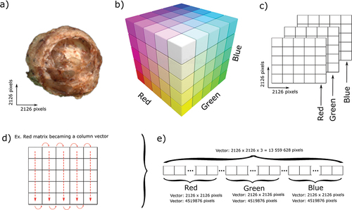
Step 1. First, each matrix of 2126 × 2126 pixels (red, green, and blue, Figure 1b,c) (Bajwa et al., 2009) were transformed into a vector by concatenating the end of each column with the beginning of the next column (Figure 1d). Then, the three new vectors (red, green, and blue) were concatenated into a single vector. Thus, each image generated a vector with one column and 13,559,628 rows. Finally, the vectors were transposed (Figure 1e) to obtain a vector of one row and 13,559,628 columns.

Step 2. All row vectors from the 16 images were put together to create a 2D matrix of 16 rows and 13,559,628 columns (Bajwa et al., 2009; Tharwat, 2016).

Step 3. PCA was performed with the new data matrix of 16 rows and 13,559,628 columns, using a covariance matrix, since the columns had the same unit values.

Step 4. The principal components found by PCA were used to carry out the HCPC (Ferreira et al., 2017). The HCPC was performed using the Euclidean distances between samples and the Ward method among groups.

2.4. Optimizing computer requirements

Two alternatives were tested to optimize computer requirements: image size reduction and conversion of the images to grayscale before reduction.

2.4.1. Image size reduction

This consisted of gradually reducing the size of the pixels in the images, resulting in images of pixel sizes 2126, 2100, 2000, 1800, 1600, 1400, 1200, 1000, 800, 600, 400, 200, 150, 100, 75, 50 and 25. Then steps 1 to 4 of Section 2.3 were applied to each reduced group of images. Additionally, we recorded total necessary to allocate the images in the computer as well as the RAM and the necessary time to perform those tasks.

2.4.2. Converting the images to grayscale and image reduction

Image processing often requires converting the original color image into a grayscale image (Igathinathane & Ulusoy, 2016). Thus, the images were converted from RGB color (3D) to a single dimension grayscale image (1D) as follows. First, each RGB matrix (where MG, MR, and MG are green, red, and blue matrixes respectively) was converted into a grayscale matrix, to obtain MRg, MGg, and MBg for green, red and blue respectively. Then the mean of the three grayscale matrixes ((MRg + MGg + MBg)/3) was calculated to obtain a single grayscale matrix (SGM) of 2126 × 21264 = 4519876 pixels. Next, that matrix was converted into a row vector by concatenating the end of each column with the beginning of the next column. Finally, steps 2 to 4 of Section 2.3 were applied. Additionally, we recorded total memory necessary to allocate the images in the computer as well as the RAM and the necessary time to perform those tasks.

2.4.3. Statistical analysis

PCA was carried out using the covariance matrix since all variables (columns: pixels) had the same order of magnitude (Rencher & Schimek, 2002), with pixel values ranging from 0 to 255, followed by HCPC using two computers, a) a supercomputer with 256 Gb of RAM; and b) a regular laptop with 8 Gb of RAM. All statistical calculations were carried out using the R statistical program version 3.6.1.

3. Results and discussion

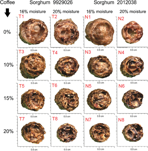
Observation of the images in Figure 2 allows distinguishing the treatments with visual similarities regarding expansion, hole sizes, image texture, and colors. The pairs T1 and N1 and T8 and N8 are similar. Another example is the images N7, T4, T3, and T6. Nevertheless, in this specific example, the classification of the same treatments using human observation was difficult, tedious and led to errors. According to Brosnan and Sun (2002), CIA presents the advantages of speed and accuracy, and thus is an attractive technique to replace human vision analysis. In this regard, since 1996, the food industry has been one of the top 10 industries to use CIA (Kakani et al., 2020).

Figure 2. Images from 16 extrusion treatments from mixes of two sorghum genotypes, four coffee powder levels, and two moisture contents.

3.1. Principal component analysis

After the PCA, the dimensionality was drastically reduced, from 13,559,628 columns to 15 new orthogonal features, called PCs, as observed in the scree plot (Figure 3). Thus, the PCA was able to reduce the data dimensionality and complexity while retaining the primary information (Zhang et al., 2022). The summarized data facilitates visualization in detail. Each PC has its robustness or amount of variance explained in its direction (Tharwat, 2016).

Figure 3. Scree plot of the 15 principal components obtained from the initial 13,559,628 variables.

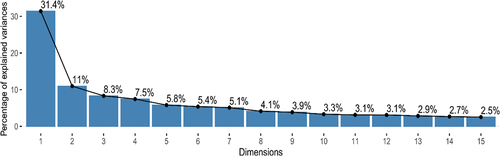
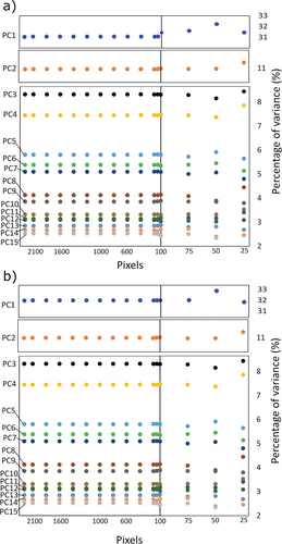
In terms of the percentage explained by the principal components (PCs, the first principal component explained 31.4% of the total variance while the second principal component explained 11% (Figures 3 and 4a). The remaining components showed a gradual small decrease, forming an “elbow”. Consequently, the two first PCs sufficiently captured the underlying phenomena, making them suitable for explanation purposes.

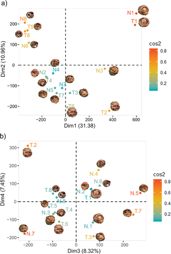
Figure 4. Principal component analysis of the original images (2126 x 2126 pixels), a) PC1 vs. PC2, b) PC3 vs. PC4.

There are different rules regarding choice of the number of principal components to represent the original dataset. This selection must take into consideration the specific phenomena being studied (Mingoti, 2005). When using a correlation matrix for PCA, some authors recommend choosing the PCs that explain a large percentage of initial variation, typically recommending values of accumulated variance explanation from 70% to 90%. Another technique is the using the screen plot and selecting the i-th components that form the referred “elbow”. Another rule is to retain the PCs with eigenvalues greater than 1 for the correlation matrix and greater than the average for the covariance matrix (Rencher & Schimek, 2002).

From the PCA here (Figure 4a,b), we grouped the treatments according to their visual similarities. The treatments N1 and T1 were placed close to each other, corresponding to 100% sorghum, 0% coffee, and 16% moisture. As the coffee content in the extrudates increased, they clustered together, aligning with their visual characteristics. Notably, samples with higher coffee content (20%) were grouped together and exhibited less expansion.

In this study, PCs 4 to 15 (Figure 3) only explained a small percentage of the variance. However, observing PC3 and PC4 (Figure 4b) indicated their minimal explanation of the similarities of the images.

Since the percentage of the explained variance was low for all PCs due to the use of the covariance matrix, and considering the successful reduction of dimensionality, we carried out HCPC analysis. HCPC is recommended because this technique uses the PC results to form clusters, thereby reflecting groups based on the total variation (Ferreira et al., 2017).

Prior to conducting HCPC, the number of clusters was determined using the NbClust function in R (Charrad et al., 2014). This function tested 30 different methods to identify the most relevant number of clusters. The NbClust function was applied using the first two PCs and all 15 PCs (total). The results indicated 3 clusters for both cases (two first PCs and all 15 PCs).

Figure 5 presents the HCPC results from the first two PCs (left) and all 15 PCs (right). The lines connecting dendrograms (red and black) indicate the location of the samples from the HCPC for the two PCs and the HCPC for all PCs. The black lines represent samples that maintained their groups and red lines indicate samples that changed. In this way, the red lines indicate that only 3 samples (T4, N4, and N2) changed group when the number of PCs used to perform the HC changed from 2 to 15 PCs.

Figure 5. Dendrogram from hierarchical clustering of principal components (HCPC) for the 16 images.

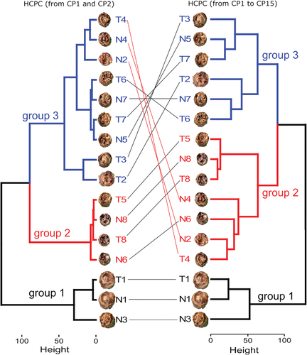
Both dendrograms were divided into three groups. Group 1, represented by the black line, consisted of the most expanded and lightest samples. Group 2 (red line), contained smaller and dark samples. Group 3 included intermediate samples in terms of expansion and color. The HC using all 15 PCs showed the best clustering, which was aligned with the human visual classification.

Based on the results of this study, we recommend using PCA followed by HCPC to achieve a classification using all PCs that represent 100% of the total variance of the phenomena.

3.2. Optimization of the computer requirements

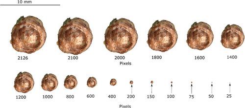
In order to implement these procedures on any computer, we conducted the same analyses (PCA and HCPC) with images that were resized from the original ones. The images were resized to various dimensions: 2126, 2100, 2000, 1800, 1600, 1400, 1200, 1000, 800, 600, 400, 200, 150, 100, 75, 50 and 25 pixels. Both color (Figure 6) and grayscale images were used in this process.

Figure 6. An example of the image reduction from the original size (2126 pixels).

The percentage of variance explained for the PCs derived from the images of different sizes remained relatively consistent, as shown in Figure 7. This trend was observed for both color and grayscale images (Figures 1a and 7b), respectively. Interestingly, the distribution of the PCs and HCPC were similar to that of the original size. This indicates image size reduction was effective until 75 pixels.

Figure 7. Percentage of the variance explained from the 15 PCs obtained applying the PCA technique for different image sizes (2126, 2100, 2000, 1800, 1600, 1400, 1200, 1000, 800, 600, 400, 200, 150, 100, 75, 50 and 25 pixels) using (a) color images and (b) grayscale images.

In terms of memory (RAM) required to store the images in the R program, Figure 8a shows that the original set of 16 color images occupied 1728 Mb. However, this declined as the images gradually decreased to 200 pixels. Beyond this threshold, the memory requirement was relatively constant. On the other hand, as expected, grayscale images required significantly less memory compared to color images. For instance, the grayscale image with 2126 pixels occupied 579.2 Mb, approximately one-third of the memory used by color images.

Figure 8. Computer memory requirements (a) to allocate the images, and (b) to carry out the PCA analysis. All calculations were performed using different image sizes (2126, 2100, 2000, 1800, 1600, 1400, 1200, 1000, 800, 600, 400, 200, 150, 100, 75, 50, and 25 pixels) using color and grayscale images.

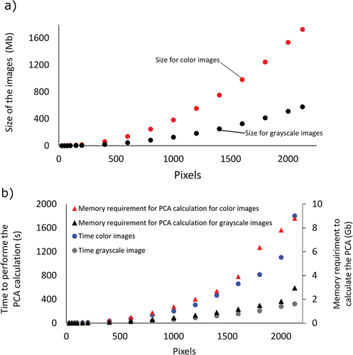
The times required to perform PCA using original images (2126 × 2126 pixels) were 1803.15 s and 323.90 s (~6 times faster) for color and grayscale respectively (Figure 8b). This means that grayscale images were approximately six times faster than color images. Furthermore, the processing time for color images decreased drastically until 1000 pixels, where it took only 203.00 s. Grayscale images also took less processing time with the size image reduction.

In addition to processing time, the amount of RAM needed to perform the calculations was also studied (Figure 7b). Color images required a greater amount of RAM, e.g. the original 2126-pixel images needing 8.8 Gb for PCA processing. In contrast, grayscale images only required approximately one-third of that amount, with 2.95 Gb being sufficient. Both color and grayscale images had lower RAM requirements with smaller the images. Thus, the use of grayscale images proved to be more advantageous in terms of computational requirements, including RAM allocation for the images, processing time, and RAM needed for PCA calculations.

3.3. Limitations of the method and feature approach

The method proposed here to group images by their similarities consisted of image size reduction and application of the statistical techniques PCA following by HCPC. This method proved to be fast and simple, allowing studies to go beyond simply describing the images and applying statistical tools. Otherwise, the numerical values of the pixels in the images will be affected, leading to inaccurate results. In future research, it would be beneficial to address this weakness.

4. Conclusion

The methods Principal Component Analysis (PCA) and Hierarchical Clustering of Principal Components (HCPC) were suitable for the study of images and could group treatments with visual similarities resulting from the extrusion of different sorghum levels (two genotypes) with coffee and two moisture levels.

By the application of these two simple multivariate statistical techniques, it was possible to determine groups based on calculations from the images instead of just visual observation. The clusterization using all PCs produced the best classification, which coincided with human visual classification. Hence, this is an easy method to classify images, with the additional advantage of low computational requirement.

Reducing the size of images resulted in the same spatial distribution in PCA and HCPC. The percentages of explained variance for all PCs was similar to the original size (2126 pixels) down to 75 pixels. The image size reduction also decreased the computational requirements and the time required to perform PCA.

There are numerous applications to image analysis using this method. For example, it can be used to classify yogurt with different levels of fruit pulp, evaluate soluble powders for beverages produced by different techniques, and the study the impact of high hydrostatic pressure on meat, among other possibilities.

Disclosure statement

No potential conflict of interest was reported by the author(s).

Additional information

Funding

This work was supported by FAPERJ grant no. E-26/204.328/2021 to Davy W.H. CH.

References

- Arboleda, E. R. (2019). Comparing performances of data mining algorithms for classification of green coffee beans. International Journal of Engineering and Advanced Technology, 8(5), 1563–1567. https://www.researchgate.net/profile/Edwin-Arboleda/publication/335104787_Comparing_Performances_of_Data_Mining_Algorithms_for_Classification_of_Green_Coffee_Beans/links/5d4fa54a299bf1995b759db0/Comparing-Performances-of-Data-Mining-Algorithms-for-Classification-of-Green-Coffee-Beans.pdf
- Bai, F., Fan, M., Yang, H., & Dong, L. (2021). Image segmentation method for coal particle size distribution analysis. Particuology, 56, 163–170. https://doi.org/10.1016/j.partic.2020.10.002
- Bajwa, I. S., Naweed, M., Asif, M. N., & Hyder, S. (2009). Feature based image classification by using principal component analysis. ICGST International Journal on Graphics, Vision and Image Processing (GVIP), 9(II), 11–17.
- Bargshady, G., Zhou, X., Deo, R. C., Soar, J., Whittaker, F., & Wang, H. (2020). Enhanced deep learning algorithm development to detect pain intensity from facial expression images. Expert Systems with Applications, 149, 113305. https://doi.org/10.1016/j.eswa.2020.113305
- Bossard, L., Guillaumin, M., & Van Gool, L. (2014). Food-101–mining discriminative components with random forests. In European conference on computer vision, Zurich, Switzerland.
- Brosnan, T., & Sun, D.-W. (2002). Inspection and grading of agricultural and food products by computer vision systems—a review. Computers and Electronics in Agriculture, 36(2), 193–213. https://doi.org/10.1016/S0168-1699(02)00101-1
- Charrad, M., Ghazzali, N., Boiteux, V., & Niknafs, A. (2014). NbClust an R package for determining the relevant number of clusters in a data set. Journal of Statistical Software, 61(6). https://doi.org/10.18637/jss.v061.i06
- Chávez, D. W. H., Ascheri, J. L. R., Carvalho, C. W. P., Godoy, R. L. O., & Pacheco, S. (2017). Sorghum and roasted coffee blends as a novel extruded product: Bioactive compounds and antioxidant capacity. Journal of Functional Foods, 29, 93–103. https://doi.org/10.1016/j.jff.2016.12.012
- Chen, J., Zhu, B., Chong-Wah, N., Chua, T. S., & Jiang, Y. G. (2021). A study of multi-task and region-wise deep learning for food ingredient recognition. IEEE Transactions on Image Processing, 30, 1514–1526. https://doi.org/10.1109/TIP.2020.3045639
- dos Santos, T. B., da Silva Freire Neto, R., Collantes, N. F., Chávez, D. W. H., Queiroz, V. A. V., & de Carvalho, C. W. P. (2022). Exploring starches from varied sorghum genotypes compared to commercial maize starch. Journal of Food Process Engineering, e14251. https://doi.org/10.1111/jfpe.14251
- Ferreira, F. S., Sampaio, G. R., Keller, L. M., Sawaya, A. C. H. F., Chávez, D. W. H., Torres, E. A. F. S., & Saldanha, T. (2017). Impact of air frying on cholesterol and fatty acids oxidation in sardines: Protective effects of aromatic herbs. Journal of Food Science, 82(12), 2823–2831. https://doi.org/10.1111/1750-3841.13967
- Han, W., Li, J., Wang, S., Zhang, X., Dong, Y., Fan, R., Zhang, X., & Wang, L. (2022). Geological remote sensing interpretation using deep learning feature and an adaptive multisource data fusion network. IEEE Transactions on Geoscience and Remote Sensing, 60, 1–14. https://doi.org/10.1109/TGRS.2022.3183080
- Igathinathane, C., & Ulusoy, U. (2016). Machine vision methods based particle size distribution of ball- and gyro-milled lignite and hard coal. Powder Technology, 297, 71–80. https://doi.org/10.1016/j.powtec.2016.03.032
- Kakani, V., Nguyen, V. H., Kumar, B. P., Kim, H., & Pasupuleti, V. R. (2020). A critical review on computer vision and artificial intelligence in food industry. Journal of Agriculture and Food Research, 2, 100033. https://doi.org/10.1016/j.jafr.2020.100033
- León-Roque, N., Abderrahim, M., Nuñez-Alejos, L., Arribas, S. M., & Condezo-Hoyos, L. (2016). Prediction of fermentation index of cocoa beans (Theobroma cacao L.) based on color measurement and artificial neural networks. Talanta, 161, 31–39. https://doi.org/10.1016/j.talanta.2016.08.022
- León-Roque, N., Aguilar-Tuesta, S., Quispe-Neyra, J., Mamani-Navarro, W., Alfaro-Cruz, S., & Condezo-Hoyos, L. (2019). A green analytical assay for the quantitation of the total saponins in quinoa (Chenopodium quinoa Willd.) based on macro lens-coupled smartphone. Talanta, 204, 576–585. https://doi.org/10.1016/j.talanta.2019.06.014
- Mingoti, S. A. (2005). Análise de dados através de métodos de estatística multivariada: uma abordagem aplicada. Editora UFMG.
- Ontoum, S., Khemanantakul, T., Sroison, P., Triyason, T., & Watanapa, B. J. (2022). Coffee roast intelligence.
- Reddy, V. H., Kumari, S., Muralidharan, V., Gigoo, K., & Thakare, B. S. (2019, May 17-18). Food recognition and Calorie measurement using image processing and convolutional neural network. In 2019 4th international conference on recent trends on electronics. Bangalore, India: Information, Communication & Technology (RTEICT).
- Rencher, A. C., & Schimek, M. (2002). Methods of multivariate analysis. Computational Statistics, 12(4), 422–422.
- Tharwat, A. (2016). Principal component analysis-a tutorial. International Journal of Applied Pattern Recognition, 3(3), 197–240. https://doi.org/10.1504/IJAPR.2016.079733
- Unal, Y., Taspinar, Y. S., Cinar, I., Kursun, R., & Koklu, M. (2022). Application of pre-trained deep convolutional neural networks for coffee beans species detection. Food Analytical Methods, 15(12), 3232–3243. https://doi.org/10.1007/s12161-022-02362-8
- Zhang, J., Li, C., Rahaman, M. M., Yao, Y., Ma, P., Zhang, J., Zhao, X., Jiang, T., & Grzegorzek, M. (2022). A comprehensive review of image analysis methods for microorganism counting: From classical image processing to deep learning approaches. Artificial Intelligence Review, 55(4), 2875–2944. https://doi.org/10.1007/s10462-021-10082-4
- Zhu, L., Spachos, P., Pensini, E., & Plataniotis, K. N. (2021). Deep learning and machine vision for food processing: A survey. Current Research in Food Science, 4, 233–249. https://doi.org/10.1016/j.crfs.2021.03.009