The Value of “Green” in Resale Residential Real Estate: Premium by Neighborhood Value Quintile, Homestead Status and Year

Abstract

This paper evaluates about 146,000 home sales from the Multiple Listing Service (MLS) of Bexar County (San Antonio), Texas, from January 2009 to April 2019 to measure the extent that a home’s selling price reflects a Green premium which is identified in the MLS. We exclude new houses from this analysis. For the span of our data, we find a 4.2% increase in the sale price of Green homes, holding other features constant. When evaluated by Area (approximate selling price quintile), we find premiums of 6.9%, 5.7%, 1.2%, 3.5%, and 5.3% by order of increasing neighborhood value quintile. When assessing Homestead versus Non-Aomestead homes, we find a premium of 2.8% for Homesteads and 6.4% for Non-Homesteads. Considering the time trend, we found the premium starting under 3% in 2009 and increasing to a little over 5% where it remained for three years and decreased to about 4% in 2014 where it remained through the end of the data in 2019.

Keywords:

• Hedonic regression analysis
• homestead
• value of green

Introduction

The value which Green features add to real estate is an ongoing area of study both for its own sake and because real estate is long-lived and a large user of energy and water. Houses with Green features may be both more comfortable and exhibit lower operating costs through energy or water efficiency. Increased insulation and multi glazed windows, for example, both increase energy efficiency, will make a home quieter and have less cycling of the heating and air conditioning (HVAC). Water-conserving landscapes may also reduce landscape maintenance time, as well as water bills. Living with a lower carbon footprint, or a Greener lifestyle may add intrinsic benefits to an owner that are not easily measured directly through energy and water saving, or less maintenance time or more home comfort. All these effects can add Green value to a home. In the fall of 2008, the San Antonio Board of Realtors^® Multiple Listing Service (SABOR MLS) added fields for listing agents to specify Green features, Green certification, and energy efficiency measures. If one or more notations were in these fields, for this paper, we set a Green indicator variable to the value one to analyze its effect on the sale price.

Literature Review

We conceptualize the literature as follows: (1) Is green important to real estate? (2) Do people indicate a willingness to pay for green in real estate? (3) How large is the premium for green features in residential real estate? Turning first to the matter of is it important, Ciochetti and McGowan (2010) summarize information from the U.S. Energy Information Administration that shows the largest user of energy in the U.S. is buildings at 41% of total consumption. They also show that the square footage of residential real estate far exceeds that of commercial buildings, and although they use less energy per square foot, in total, they consume the most energy. Sewalk and Throupe (2014) examine the costs in Denver to bring existing homes up to current energy efficiency standards and find the costs exceed the projected benefits. They also find, however, that adding insulation and using energy-efficient appliances and lighting when replacing the current items is cost-effective.

Considering the second question of whether people are willing to pay a premium, Goodwin (2011) studied the demand for Green amenities and determined that buyers of new homes are more interested in Green amenities than those purchasing resales. She also found buyers under age 40 and buyers with incomes over $100,000 were less interested in Green features. Levinson (2016) questions why residential building energy codes never save the amount of energy that the codes predict. He states, “Plus, new and old buildings might use similar amounts of energy today because residents of efficient houses respond to the lowered cost of lighting, air conditioning, and heating by using more: the so-called “rebound” effect. In that case, the codes may make homeowners warmer in winter and cooler in summer but not save as much energy as promised.” This result does not mean owners do not value the Green improvements. Owners may make improvements on existing structures that could exceed requirements. Those who prefer to keep their homes very warm in winter and very cool in summer may use much energy and value Green improvements highly as the financial consequences of their comfort is dampened.

Exploring the answer to the third question is the crux of this paper—“How is Green valued in the residential single family market?” This is an essential question for residential real estate appraisers, real estate agents, and developers. One approach to addressing this question, when there are direct dollar savings, is to take the present value of these savings as an estimate of the increased value. Adomatis (2010), for example, outlines this approach in a residential context. She follows this up with a more comprehensive paper describing a more extensive set of Green improvements (Adomatis, 2012). This study, however, like a number of previous studies, seeks a direct measure of the increase in sales price from green features. Table 1 summarizes eight papers that have directly addressed this question. This table notes the paper, the location and study objective, the data sample, and the green premium that is measured. Green premiums were measured in the 2.5-5.9% for most of these papers.

Table 1. Summary of recent studies of the green sales premium in residential real estate.

Author	Location/concern	Sample	Value of Green
Bloom et al. (2011)	Fort Collins CO Value of Energy Star Rating	“Newer Homes” sold between 1999 and 2005: 150 Energy Star homes, 150 other homes. Dependent variable was Sales price per sqft.	Energy Star homes sold for $8.66 more per sqft. (Average Price not provided so could not convert to percent)
Aroul & Hansz (2011)	Clovis, CA Value of dual pane windows	Mostly existing homes sales during 2008–2010. N = 3704 with almost 40% of sample having dual pane windows.	3% higher resale value for homes with dual pane windows
Aroul & Hansz (2012)	Frisco, and McKinney, TX (Dallas-Ft. Worth MSA) Value of Green building program implemented in Frisco	Frisco required new plats after 2001 to implement green building program, while similar city McKinney did not. N = 14,055 with approximately half in each city with 48% sales being green. New to 8 year old houses with average age of 3.3 years.	Mandatory green adds 3 - 5% increased selling price depending on sample used. Optional green investments value was lower (0.2–1.1%)
Dastrup et al. (2012)	San Diego and Sacramento, CA Value of Solar System	Data from Jan 1997-Dec 2010. San Diego 329 sales with solar system and 364,663 sales without. Sacramento 265 sales with and 90,686 sales without.	San Diego: 3.6% gain in sale price (predicted $22,554 amount). Sacramento 4% gain
Cadena & Thomson (2015)	San Antonio, TX Value of green features	New and used homes sold during Oct 2008–Sep 2013. N = 66,000 sales with about 50% percent green.	5.9% overall green premium.
Pride et al. (2017)	Anchorage, AK Value of energy efficient upgrades	Used Homes: N = 2,791 repeat sales during 2008–2015, for which 220 participated in the energy efficiency program between sales	4.2% premium for energy improvement program
Aroul & Rodriguez (2017)	Frisco TX, (part of Dallas Forth Worth MSA) Value of Green building designation	Green Building program required if platted after 2001. N = 25,272 sales from Jan 2002-Dec 2009, with 44% of sales designated Green	No premium first 2 years, then increasing to 2.5% for 2007–2009. Overall premium 2.27%
Ma & Narwold (2019)	San Diego, CA Value of orientation to the sun	Evaluated homes by directional siting of house (8 categories of the 4 cardinal and 4 intercardinal directions). N = 26,749 in full sample. N = 241 for custom homes on lots larger than ½ acre.	Results depend on sample used. No gain found for lower valued (bottom 72%) of sales. Gains up to a12.8% premium for Southeast orientation for custom houses on large lots.
This study	San Antonio, TX Value of green features in residential resale	Resale homes sold from Jan 2009 to May 2019. N = 146,000, 35% of sample noted green.	4.2% green premium overall

Research Questions and Hypotheses

The papers noted in Table 1 address the value green brings to residential real estate. Ma and Narwold (2019) found that to detect a premium for the value of house orientation they had to limit their sample to higher valued houses, using the sense that for tract houses on small lots, orientation is not an important concern to purchasers. They found the largest values when they restricted their results to custom houses on large lots. We propose a much simpler approach that addresses a related question—is the value of green dependent on the average house value in the neighborhood the house is sited in?

Our second extension to existing research is to determine whether the value of green depends on whether sale if by owner occupant or not. To our knowledge this question has not been addressed in previous research. Our third extension follows Aroul and Rodriguez (2017) in addressing whether green values change over time. Our first extension of Aroul and Rodriguez is to pick up, time wise, where they leave off and to continue to a more recent date. We have a longer time horizon to address this question. We also address whether the Green Area effect and Green Homestead effect is stable over time. In summary this paper addresses whether the green premium varies among neighborhood value quintiles (Area), varies by homestead status at time of sale, or varies over time. We do not have strong priors regarding any of these research questions and thus our research hypotheses are general.

Hypothesis 1. The Green premium is the same (percentwise) among value stratified neighborhoods.

Hypothesis 1A: The Green premium is not the same (percentwise) among value stratified neighborhoods.

One could conjecture that in lower priced neighborhoods incomes are constrained so that anything that lowers housing costs (such as energy efficiency) will be highly valued and capitalized into the selling price of the house. For high priced neighborhoods, costs savings could be less than important the psychic benefits from living a greener lifestyle for those who have the means and choose to own houses with green features. It is also possible that for house purchasers for whom green is important, their actions will create a green premium that is similar across neighbor value. To test this hypothesis, we segment the MLS neighborhoods into approximate value quintiles (Areas) to determine whether the premium varies by Area.

Hypothesis 2: Green premium does not vary by the ownership status of the house being purchased.

Hypothesis 2A: Green premium varies by the ownership status of the house being purchased.

Home purchasers may not be aware of the ownership status when purchasing, but the ownership may affect the combination of features the house offers which may affect the green premium. We evaluate this hypothesis by determining the homestead status of the house at the time of sale and evaluating the premium for Homestead versus Non-Homestead status.

Hypothesis 3: Green value is constant over time.

Hypothesis 3A: Green value is not constant over time.

Although recognizing green value is not new, our data starts in 2009 when green may have been coming into its own. Aroul and Rodriguez (2017) end their data in 2009 and showed an increasing trend over time that was leveling off by the end of their data. While the green premium cannot increase indefinitely it could fluctuate over time. Also, just prior to 2009 is when the MLS used in our study added the new green fields to the database, so there may be a period for real estate agents to become familiar with the new fields and to employ them when listing a house for sale. This could affect our results in the early period. An additional possibility is that green may be more, or perhaps less, important in a flat real estate market, as was observed after the great real estate recession brought on by the subprime mortgage crisis. As markets returned to full health a wider spectrum of houses may be on the market which could affect the value of green. Another possibility is that green could be somewhat of a fad, and have some short lived value, or it could show some shorter term excitement (high value) before settling in at a long term value. Overall we remain agnostic as to what the analysis will show. To test for any time trend, we run annual regressions on the data to determine whether the value of green changes over time. We also run regressions on Area and Homestead status over time to determine whether Green premiums related to these measures are constant over time.

Data

Our data is primarily drawn from the San Antonio Board of Realtors^® Multiple Listing Service (SABOR MLS). This provides the sale price, date of sale, the time on market, and associated information about the house and other potentially relevant information regarding the sale, such as source of financing. Three new fields were introduced into this data set in October of 2008, and it is from these new fields we extract our green identifier. These new fields are labelled “Green Designations,” “Green Features,” and “Energy Efficient Features.” Using earlier data, Cadena and Thomson (2015) evaluated these fields and found that parsing this data into one “Green” identifier provide the most consistent result. We follow this approach and if there is an entry into any of these fields we set the Green identifier to one. Cadena and Thomson reported that almost 97% of new homes exhibit Green features; thus, we exclude new homes from the analysis presented here. Given that distressed properties may not fully reflect the values of typical transactions, we also removed short sales and foreclosure sales from this analysis.

To investigate the green premium for homes designated as the owner’s principal residence at their time of sale compared to other homes (primarily rental units) we required a second data source. In the State of Texas, a homeowner may declare their primary residence a homestead.

There are no specific qualifications for the general homestead exemption other than the owner has an ownership interest in the property and uses the property as the owner’s principal residence. However, an applicant is required to state the applicant does not claim an exemption on another residence homestead inside or outside of Texas.¹

Homestead status adds legal protections to the property that non-homesteads do not enjoy. More important for most homeowners, however, is that if they declare homestead status to the local appraisal district, they receive some mandated property tax relief. The amount of relief in taxes varies by taxing jurisdiction, as the dollar amount of an exemption may vary for a school district, city, or other taxing authority. In Bexar County, the annual property tax savings will typically be in the $200–400 range per year. In times of rapidly increasing property values, declared homesteads are limited to an annual increase in taxable value of 10%, which may provide further property tax relief due to the homestead declaration. In addition, homeowners over 65 or disabled qualify for additional property tax relief. These financial benefits provide a strong incentive for homeowners to declare their primary residence as a homestead. To aid in this process, a notice is sent with the property tax appraisal to new owners informing them that, if they qualify, they may apply for the homestead exemption.

Non-homestead declared houses generally fall into one of three categories: (1) Rental Property, (2) Second Home Property, or (3) Owner-occupied principal residence that did not apply for the homestead exemption. Because of the adverse financial consequences of (3), we expect few properties that qualify for the homestead exemption would fail to apply for it². We assume most non-homestead homes are rental properties, and this to be especially true in the low and moderate house price areas where the localized economic profile may prevent a high proportion of homeowners.

We were able to purchase Bexar County Appraisal District data for the period of our analysis that allows us to determine the homestead status of each property on January 1 of each year. For every sale, we were able to cross-reference its homestead status using this data and merge this into our home sale data set.

We examined our data for nonsensical values and other coding errors and removed these observations from our data. Extreme outliers in terms of house price or size, are not cogent to this analysis and were also eliminated. Table 2 presents the descriptive statistics for our data. House prices in our dataset range from $20,000 to $2,000,000 with an average selling price of $207,000; size ranges from 300 to 12,000 square feet with an average size of 2,100 square feet; and age ranges from two to 143 years with an average age of 27 years. Because some new homes are completed near the end of the year and sold the next, they are computed (Age = Year Sold – Year Built) to be 1-year-old when they are in fact new; thus, we start our analysis using home computed to be at least 2 years old. Overall, in our data, 35% of sales are designated Green and 55% are Homesteads. The average time on market (TOM) is 73 days (0.199 years). We present many covariates that describe the house such as size, age, number of bathrooms, garage spaces, indicator for single story and whether or not it has a swimming pool. We provide further information about the house including exterior cladding, style, type of roof, HVAC, flooring, and foundation. Also included is other information related to the transaction such as whether the house had a recent rehab, needs tender loving care, was vacant or leased, whether it was part of a required home owner association, whether it was broker or agent owned, and how the sale was financed. For attributes described via several indicators such as flooring, HVAC, or financing, the most common indicator is not reported and its effect will be part of the regression intercept.

Table 2. Variable names and descriptive statistics (N = 145,983).

Variable name	Mean	StDev	Min	Max
Sale Price	206,710	135,958	10,000	2,000,000
Log(Sale Price)	12.075	0.573	9.210	14.509
Green	0.347	0.476	0.000	1.000
Green-Area1	0.021	0.145	0.000	1.000
Green-Area2	0.097	0.295	0.000	1.000
Green-Area3	0.079	0.270	0.000	1.000
Green-Area4	0.089	0.285	0.000	1.000
Green-Area5	0.061	0.239	0.000	1.000
Green-HomeStd	0.232	0.422	0.000	1.000
Green-NotHomeStd	0.116	0.320	0.000	1.000
GrnArea1-HS	0.011	0.104	0.000	1.000
GrnArea1-NotHS	0.011	0.102	0.000	1.000
GrnArea2-HS	0.060	0.238	0.000	1.000
GrnArea2-NotHS	0.036	0.186	0.000	1.000
GrnArea3-HS	0.053	0.223	0.000	1.000
GrnArea3-NotHS	0.026	0.161	0.000	1.000
GrnArea4-HS	0.065	0.247	0.000	1.000
GrnArea4-NotHS	0.024	0.153	0.000	1.000
GrnArea5-HS	0.042	0.202	0.000	1.000
GrnArea5-NotHS	0.019	0.135	0.000	1.000
Time On Mkt (Yr)	0.199	0.201	0.003	1.052
Homestead	0.554	0.497	0.000	1.000
SqFt (1000)	2.103	0.822	0.300	12.000
Total Baths	2.556	0.860	1.000	10.000
Garages	2.074	1.183	0.000	9.000
Age (Years)	26.627	21.617	2.000	146.000
One Story	0.547	0.498	0.000	1.000
Swim Pool	0.096	0.294	0.000	1.000
Exterior Aluminum	0.004	0.059	0.000	1.000
Exterior Asbestos	0.047	0.211	0.000	1.000
Exterior Masonry	0.309	0.462	0.000	1.000
Exterior Siding	0.244	0.430	0.000	1.000
Exterior Stone	0.092	0.289	0.000	1.000
Exterior Stucco	0.075	0.263	0.000	1.000
Exterior Vinyl	0.026	0.160	0.000	1.000
Exterior Wood	0.127	0.333	0.000	1.000
Style Historic	0.018	0.134	0.000	1.000
Style Mediterranean	0.016	0.126	0.000	1.000
Style Ranch	0.047	0.211	0.000	1.000
Style Split Level	0.012	0.108	0.000	1.000
Style Traditional	0.243	0.429	0.000	1.000
Style Colonial	0.003	0.056	0.000	1.000
Style Contemporary	0.102	0.303	0.000	1.000
Roof Metal	0.024	0.154	0.000	1.000
Roof Other	0.011	0.103	0.000	1.000
Roof Tile	0.026	0.158	0.000	1.000
HVAC No AC	0.021	0.144	0.000	1.000
HVAC Window AC	0.026	0.159	0.000	1.000
HVAC Zoned	0.025	0.155	0.000	1.000
Floor Carpet	0.781	0.413	0.000	1.000
Floor Ceramic	0.713	0.453	0.000	1.000
Floor Laminate	0.077	0.266	0.000	1.000
Floor Linoleum	0.098	0.297	0.000	1.000
Floor Marble	0.009	0.093	0.000	1.000
Floor Parquet	0.005	0.068	0.000	1.000
Floor Stained Concrete	0.002	0.047	0.000	1.000
Floor Slate	0.003	0.053	0.000	1.000
Floor Saltillo Tile	0.033	0.179	0.000	1.000
Floor Vinyl	0.073	0.261	0.000	1.000
Floor Wood	0.123	0.328	0.000	1.000
Foundation Pier-Beam	0.068	0.251	0.000	1.000
Recent Rehab	0.149	0.356	0.000	1.000
Needs TLC	0.023	0.150	0.000	1.000
Vacant	0.405	0.491	0.000	1.000
Currently Leased	0.034	0.180	0.000	1.000
HOA Mandatory	0.580	0.493	0.000	1.000
Broker Agent Owned	0.058	0.234	0.000	1.000
Financed Cash	0.176	0.380	0.000	1.000
Financed FHA	0.259	0.438	0.000	1.000
Financed Other	0.014	0.119	0.000	1.000
Financed VA	0.162	0.369	0.000	1.000

After the dependent variable (Log(Sale Price), Variables are organized as follows: Green Indicator Variable; Green Indicator interacted with Area; Green Indicator interacted with Homestead, Green Indicator interacted with Area and Homestead; Time on Market; Homestead Indicator; basic house characteristics; extended set of physical house characteristics (exterior cladding, style, flooring, etc.); condition variables (recent rehab or needs tender loving care); additional information regarding occupancy status; and how the sale was financed. Not presented are Monthly Indicator Variables.

To study whether green has the same value across neighborhoods, we grouped the 49 MLS recognized neighborhoods by ranking their average sales price and then created approximate quintiles based on the average sale price, which we refer to as Areas. Because we wanted to retain as many observations as possible in each area we did not employ any formal clustering analysis, but instead used the straightforward procedure of grouping neighborhoods by average selling price. Table 3 presents some descriptive data about these areas illustrating there remains a large range of sale prices, but the mean and median are distinct among areas. We also see that green is more common in the higher valued Areas (though this paper addresses its value rather than its frequency) and that homestead homes are also more common in the higher value areas. The average sale price, by approximate quintile is: Area1=$115,000; Area2=$151,000; Area3=$184,000; Area4=$272,000; and Area5=$345,000. While this table shows both homestead and green frequency, it does not show their interaction. While Green is 35% of all data, Green is present for 26% of Non-Homesteads and 42% of Homesteads.

Table 3. Summary information for approximate value quintile areas.

		House Sale Price
Area	MLS Area ID	N	Average	Median	Minimum	Maximum	StDev	Pct Green (%)	Pct HS (%)
1	700, 2200, 1200, 2100, 1900, 2300, 2302, 800 , 2003, 2304, 1700	2,5827	114,599	110,000	10,000	740,000	57,228	18	38
2	1500,2004, 1600, 200, 300	3,7012	150,904	147,000	15,000	1,230,000	51,498	31	53
3	2301, 2001, 2900, 2002, 2303, 103, 400, 100, 1400, 101, 900	3,0382	184,083	170,000	20,000	1,900,000	91,538	34	56
4	1100, 104, 102, 3100, 105, 1802, 1804, 500, 600, 1001, 1000	2,9887	272,172	244,000	12,000	1,960,000	133,347	46	66
5	1803, 1801, 1005, 1300, 1002, 1006, 2800, 2705, 1004, 1003	2,2916	345,093	305,000	20,000	2,000,000	188,425	47	64

Area 1 are lowest valued neighborhoods and Area 5 are highest. In addition to information on Sale Price, the Percent of Sales that were indicated as Green, and the Percent of Sales which were Homesteads is also reported.

Methods

Valuation of residential properties and the features that add or subtract to their value is an ongoing topic of interest in real estate. Following an influential early paper on hedonic valuation by Rosen (1974), a hedonic approach to valuation has taken hold in real estate. Rosen (2002) in his section on interpreting the implicit value of characteristics, states “The hedonic regression method regresses product prices on product characteristics…. In land and housing markets, site and structure prices are regressed on house attributes (size, architectural style, and age) and on-site characteristics…”) Malpezzi (2003) and Chin and Chau (2003) review hedonic house pricing studies and summarize their structure and their applications to locational, structural, and neighborhood factors that influence housing values. Herath and Maier (2010) reviewed 471 papers that address hedonic price models for real estate and housing studies. They note that 178 of these consider neighborhood factors and a further 16 consider property characteristics. Dastrup et al. (2012) note, “In reality, homes are differentiated products that differ along many dimensions. No home has a ‘twin.’” Hedonic pricing models were employed for most of the literature previously noted where the value of Green characteristics was estimated.

We employ a series of standard hedonic pricing models similar to those used other in real estate valuation research. Some of our models disaggregate our data by year. Our model uses the semi-log form: (1) $$\mathrm{Ln}{\left(\text{Sale Price}\right)}_{\mathrm{i}}=f ({\mathrm{G}}_{\mathrm{i}},\mathrm{ }{\mathrm{A}}_{\mathrm{i}},\mathrm{ }{\mathrm{H}}_{\mathrm{i}},\mathrm{ }{\mathrm{CV}}_{\mathrm{i}},\mathrm{ }{\mathrm{M}}_{\mathrm{i}})$$(1) where: Ln(Sale Price)_i is the natural log of the House Sale Price; G_i is a Green indicator value; A_i is a vector of Area neighborhood value quintile indicators (Areas); H_i is an indicator of homestead status. CV_i is a vector of control variables frequently used in hedonic real estate studies. M_i is a vector of monthly indicator variables to capture time trend in value.

As is common in such models, we use the Log of Sales price, rather than Sales price as the dependent variable. By using the log of house price, we can interpret indicator variable coefficients as the percentage effect on sales prices; thus, the results apply across a spectrum of home prices. If a Green coefficient is 0.05, it means when the green feature is present, the house will sell for about 5% more. We estimate our models using Ordinary Least Squares regression.

Because Green features may be part of several features common to high -quality houses, we constructed an extensive set of control variables to prevent the Green indicators from simply indicating a highly valued house. If we simply compare the average price of houses with some type of Green feature to the average price of those without, we find the Green homes sell for approximately 27% more than houses without Green features ($248,000 v. $186,000). Green homes are larger (2340 square feet v. 1980) and newer (21.3 years v. 29.5 years), which in part describes their higher sale value. This quick check illustrates the need to have a complete set of covariates to isolate the Green effect from other desirable features a house may exhibit.

There has been some discussion regarding hedonic model specification. Pride et al. (2017) note that the hedonic framework has been criticized. They state that Chin and Chau (2003) note they are often misspecified by either including irrelevant variables or omitting relevant variables. Hedonic models will not include everything that may affect house value, so a reasonable question is whether this leads one astray in making inferences. Butler (1982) states,

The purpose of this paper is to fill part of that gap by examining briefly the theoretical and empirical parameters of an ‘approximately correct specification,’ and to present some evidence that approximate correctness can be achieved with significantly fewer characteristics than is generally supposed… . Given that the arguments of the hedonic function must be limited to housing characteristics, the natural next question is: which housing characteristics? In principle, all characteristics relevant to the determination of market price-i.e., those that both yield utility to residents and are costly to produce- should be included. In practice, this cannot be done because the number of such characteristics is unmanageably large. Data on many of these are either unavailable or of exceedingly poor quality.

Butler estimates a hedonic model with four covariates, and another that adds six additional covariates for which three are not statistically significant. He then analyses the modeled pricing errors with both models and concludes that either model works well. Butler does not try to make inferences about how accurate the assessment of the effect of each of the covariates is—which is what we wish to do in this study. In other words, the purpose of this study is not to determine whether we accurately predict selling price overall, but in estimating an accurate measure of the Green premium.

We examine whether the inclusion of a large number of housing characteristics matter for accurately estimating the Green premium. We first employ a “Basic” model to estimate the Green premium, and then estimate with our full model that includes many more covariates. We provide results that demonstrate that without a deeper level of control variables, the value to Green could be substantially overestimated.

Two other potential concerns are considered here. One is that Green, to the extent it is a desirable feature may be highly correlated with other desirable features leading to imprecise measures of the Green effect. A way to detect whether this correlation is a problem is through the Variance Inflation Factor (VIF). The VIF’s are reported along with the parameter estimates and they are low for our green estimates in all models presented (never higher than 1.9) so collinearity is not deemed a concern for the reported results.

A second concern is that Green is also known to affect time on market (TOM); thus, time on market should be controlled for in our models. When possible, this would be corrected via a 2-stage approach. We estimated a time on market model and used it to create a predicted time on market to use as a covariate in our models. The VIF was above 160 for this variable when it was included in our estimated model; therefore, we include the actual time on market as a covariate and results presented in Tables 4 and 5 show its VIF is low (less than 1.7).

Table 4. Ordinary least squares regression results summary for basic model.

Panel A: Green as single indicator variable
	ParamEst	StdErr	t-val	Pval	VIF	95% Confidence
Intercept	10.842	0.014	768.710	<.0001	0.000	10.815–10.870
Green	0.082	0.002	52.780	<.0001	1.098	0.079–0.085
Area1	−0.365	0.002	−154.500	<.0001	1.622	−0.369 to −0.360
Area2	−0.136	0.002	−64.840	<.0001	1.677	−0.141 to −0.132
Area4	0.119	0.002	51.920	<.0001	1.709	0.114–0.123
Area5	0.230	0.003	91.090	<.0001	1.688	0.225–0.235
TOM	−0.010	0.004	−2.620	0.009	1.157	−0.017 to −0.002
Homestead	0.060	0.001	40.180	<.0001	1.099	0.057–0.063
SqFt (1000)	0.360	0.002	222.260	<.0001	3.543	0.357–0.363
Total Baths	0.095	0.002	59.490	<.0001	3.762	0.092–0.098
Garages	0.009	0.001	15.060	<.0001	1.048	0.008–0.010
Age	0.000	0.000	−6.720	<.0001	1.405	0.000–0.000
One Story	0.156	0.002	80.310	<.0001	1.875	0.152–0.160
Swim Pool	0.121	0.003	47.040	<.0001	1.152	0.116–0.126
Panel B: Green Indicators separated by value quintile Area
Green-Area1	0.169	0.005	33.210	<.0001	1.084	0.159–0.179
Green-Area2	0.105	0.003	39.530	<.0001	1.229	0.100–0.110
Green-Area3	0.048	0.003	16.290	<.0001	1.254	0.042–0.053
Green-Area4	0.058	0.003	19.600	<.0001	1.407	0.052–0.063
Green-Area5	0.079	0.004	21.590	<.0001	1.533	0.072–0.086
Panel C: Green Indicators separated by Homestead status
Green-HomeStd	0.055	0.002	28.220	<.0001	1.369	0.051–0.059
Green-NotHomeStd	0.125	0.002	50.930	<.0001	1.236	0.120–0.130
Homestead	0.083	0.002	45.980	<.0001	1.599	0.079–0.086

Dependent Variable Log of Sale Price. N = 145,983. All models below Adjusted R-square = 0.778. Monthly Indictor variables not displayed.

Table 5. Ordinary least squares regression results summary for full model.

	ParamEst	StdErr	t-val	Pval	VIF	95% Confidence
Panel A: Green as single indicator variable. Adjusted Rsquare = 0.8425.
Intercept	10.992	0.012	889.320	<.0001	0.000	10.967–11.016
Green	0.042	0.001	31.670	<.0001	1.164	0.039–0.044
Area1	−0.273	0.002	−135.41	<.0001	1.731	−0.277 to −0.269
Area2	−0.112	0.002	−63.950	<.0001	1.719	−0.116 to −0.109
Area4	0.111	0.002	58.180	<.0001	1.743	0.107–0.115
Area5	0.200	0.002	93.930	<.0001	1.770	0.196–0.205
TOM	−0.026	0.003	−8.330	<.0001	1.169	−0.032 to −0.020
Homestead	0.031	0.001	24.170	<.0001	1.225	0.029–0.034
SqFt (1000)	0.317	0.001	227.730	<.0001	3.853	0.315–0.320
Total Baths	0.062	0.001	46.350	<.0001	3.882	0.059–0.065
Garages	0.007	0.001	13.750	<.0001	1.052	0.006–0.008
Age	0.000	0.000	3.600	0.000	3.900	0.000–0.000
One Story	0.126	0.002	75.260	<.0001	2.029	0.122–0.129
Swim Pool	0.101	0.002	46.580	<.0001	1.183	0.096–0.105
Exterior Aluminum	−0.142	0.010	−14.230	<.0001	1.017	−0.161 to −0.122
Exterior Asbestos	−0.098	0.003	−31.820	<.0001	1.254	−0.105 to −0.092
Exterior Masonry	0.021	0.002	13.280	<.0001	1.549	0.018–0.024
Exterior Siding	−0.043	0.002	−27.600	<.0001	1.309	−0.046 to −0.040
Exterior Stone	0.023	0.002	10.540	<.0001	1.129	0.018–0.027
Exterior Stucco	0.058	0.002	23.220	<.0001	1.261	0.053–0.063
Exterior Vinyl	−0.071	0.004	−19.030	<.0001	1.042	−0.078 to −0.064
Exterior Wood	−0.058	0.002	−28.710	<.0001	1.312	−0.062 to −0.054
Style Historic	0.244	0.005	49.340	<.0001	1.293	0.234–0.253
Style Mediterranean	0.059	0.005	11.200	<.0001	1.284	0.049–0.069
Style Ranch	0.052	0.003	17.750	<.0001	1.105	0.046–0.057
Style Split Level	0.070	0.005	12.740	<.0001	1.025	0.059–0.081
Style Traditional	0.016	0.001	11.020	<.0001	1.143	0.013–0.019
Style Colonial	0.105	0.011	9.980	<.0001	1.010	0.084–0.125
Style Contemporary	0.020	0.002	9.840	<.0001	1.096	0.016–0.024
Roof Metal	0.153	0.004	38.870	<.0001	1.082	0.145–0.160
Roof Other	0.043	0.006	7.390	<.0001	1.020	0.031–0.054
Roof Tile	0.142	0.004	33.310	<.0001	1.322	0.133–0.150
HVAC No AC	−0.544	0.005	−120.47	<.0001	1.246	−0.552 to −0.535
HVAC Window AC	−0.290	0.004	−71.250	<.0001	1.222	−0.297 to −0.282
HVAC Zoned	0.028	0.004	7.220	<.0001	1.072	0.020–0.036
Floor Carpet	0.031	0.002	15.070	<.0001	2.067	0.027–0.035
Floor Ceramic	0.055	0.002	24.960	<.0001	2.924	0.051–0.059
Floor Laminate	0.027	0.003	9.990	<.0001	1.565	0.022–0.033
Floor Linoleum	−0.063	0.003	−23.420	<.0001	1.878	−0.068 to −0.058
Floor Marble	0.123	0.007	18.820	<.0001	1.081	0.110–0.136
Floor Parquet	0.046	0.009	5.290	<.0001	1.028	0.029–0.063
Floor Stain Concrete	0.119	0.013	9.410	<.0001	1.052	0.094–0.144
Floor Slate	0.131	0.011	11.690	<.0001	1.024	0.109–0.152
Floor Saltillo Tile	0.099	0.004	25.940	<.0001	1.361	0.091–0.106
Floor Vinyl	−0.050	0.003	−17.470	<.0001	1.610	−0.055 to −0.044
Floor Wood	0.110	0.002	44.340	<.0001	1.946	0.105–0.115
Fndation Pier Beam	0.086	0.003	27.110	<.0001	1.859	0.080–0.092
Recent Rehab	0.078	0.002	44.470	<.0001	1.137	0.074–0.081
Needs TLC	−0.069	0.004	−17.450	<.0001	1.046	−0.077 to −0.061
Vacant	−0.056	0.001	−42.080	<.0001	1.241	−0.058 to −0.053
Current Leased	−0.044	0.003	−13.120	<.0001	1.059	−0.050 to −0.037
HOA Mandatory	0.037	0.002	20.490	<.0001	2.389	0.034–0.041
Broker Agent Owned	0.022	0.003	8.660	<.0001	1.038	0.017–0.027
Financed Cash	−0.168	0.002	−94.460	<.0001	1.346	−0.172 to −0.165
Financed FHA	−0.029	0.002	−18.210	<.0001	1.386	−0.032 to −0.025
Financed Other	−0.062	0.005	−12.450	<.0001	1.034	−0.072 to −0.052
Financed VA	−0.013	0.002	−7.320	<.0001	1.237	−0.016 to −0.009
Panel B: Green indicators separated by value quintile Area. Adjusted Rsquare = 0.8487
GreenArea1	0.069	0.004	16.250	<.0001	1.100	0.060–0.077
GreenArea2	0.057	0.002	25.660	<.0001	1.260	0.053–0.061
GreenArea3	0.012	0.002	4.910	<.0001	1.278	0.007–0.017
GreenArea4	0.035	0.002	14.440	<.0001	1.432	0.031–0.040
GreenArea5	0.053	0.003	17.470	<.0001	1.553	0.047–0.059
Panel C: Green indicators separated by Homestead status. Adjusted Rsquare = 0.8487
Green-HS	0.028	0.002	17.140	<.0001	1.417	0.025–0.031
Green-NotHS	0.064	0.002	31.050	<.0001	1.276	0.060–0.068
Homestead	0.043	0.002	27.890	<.0001	1.739	0.040–0.046
Panel D: Green Premium for Indicators Variables separated by Area and Homestead status. Adjusted Rsquare = 0.8491 (Grn: Green; HS: Homestead; NotHS: Not Homestead)
GrnArea1-HS	0.050	0.006	8.32	<.0001	1.130	0.038–0.061
GrnArea1-NotHS	0.081	0.006	13.68	<.0001	1.086	0.070–0.093
GrnArea2-HS	0.044	0.003	15.37	<.0001	1.382	0.039–0.050
GrnArea2-NotHS	0.071	0.003	20.68	<.0001	1.203	0.064–0.078
GrnArea3-HS	0.003	0.003	1.05	0.294	1.371	−0.003–0.009
GrnArea3-NotHS	0.028	0.004	6.87	<.0001	1.234	0.020–0.036
GrnArea4-HS	0.029	0.003	9.83	<.0001	1.535	0.023–0.034
GrnArea4-NotHS	0.052	0.004	11.64	<.0001	1.359	0.043–0.060
GrnArea5-HS	0.039	0.004	10.50	<.0001	1.666	0.032–0.046
GrnArea5-NotHS	0.088	0.005	16.89	<.0001	1.452	0.078–0.098
Area1-HS	0.066	0.003	21.42	<.0001	1.775	0.060–0.072
Area2-HS	0.043	0.003	16.04	<.0001	2.477	0.038–0.048
Area3-HS	0.035	0.003	11.85	<.0001	2.708	0.029–0.041
Area4-HS	0.039	0.003	11.78	<.0001	3.802	0.033–0.046
Area5-HS	0.018	0.004	4.70	<.0001	4.010	0.011–0.026

Dependent Variable Log of Sale Price. N = 145,983. Monthly Indictor variables not displayed.

Results

Thirty-five percent of our sales exhibit the Green indicator. Looking more closely, we find (Figure 1) that in our first year of data, about 23% of sales had a Green indicator. This presence increased through 2015 when it reached 38% of sales before dropping to about 34% of sales. It may be that it took a few years for real estate agents to take advantage of the Green fields in the MLS, leading to the increase in Green identified houses after the early data period. Our data shows the average age of home sales increasing over the decade. Our data also shows that older houses are less likely to be Green. The combination of these facts may explain the small downward trend in Green in more recent years.

Figure 1. Proportion of sales with Green Indicator by year. Panel A. All Areas. Panel B. By Area.

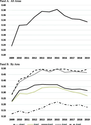
Figure 1, Panel B, disaggregates the annual data by neighborhood value quintile (Area). We note here that the median age of sale is highest in Area1 (44 years) and shows lower values for the other quintiles (24, 27, 20, 23 years). We have already noted that Green is more common in newer homes. The lowest valued quintile (Area 1) shows the lowest proportion of Green sales—starting at about 12% and increasing through 2015 after which it levels at about 20% of sales. Area2 and Area3 start about 22%, increase to about 35% and then fall to about 30%. Area4 and Area5 start out about 30% and increase to about 50% by 2013 where they remain.

We begin our hedonic regression analysis with a set of house characteristics commonly used in such models, plus neighborhood value quintile indicators, and month of sale indicator variables (Basic Model). Table 4 shows that for this model with the full 145,983 observations, the Green coefficient is 0.082 (p < 0.0001), and the Adjusted R-square is 0.778, demonstrating this model explains much of the variation in sale price. TOM is a statistically significant variable (homes that sell quicker sell for more), as are all of the included covariates. An innovation in this paper is to evaluate the homestead effect for green, so it is useful to note that the Homestead parameter estimate is 0.06 demonstrating that Homestead houses sell for more than Non-Homesteads. The highest variance inflation factors (VIF) are for house size and number of bathrooms. It is reasonable to expect that larger houses will have more bathrooms. We computed the correlation between these two variables as 81%. Our goal in this paper is not to separate the influence of square feet versus number of bathrooms so the somewhat higher variance inflation for these variables is not a concern for this paper.

To begin assessing our first hypothesis, that is, to determine whether the green effect is constant by neighborhood value quintile, we interact the Area variables with the Green variable to create five green by area variables and rerun our regression including these in place of the single Green variable. These results, presented as Panel B Table 4, shows Green is most valuable in the lowest valued neighborhoods (near 17%) and lowest in the middle quintile area (about 5%). The other Area quintiles show a Green premium of about 6-11%.

To address our second hypothesis, the value of green by homestead status, we run a model that interacts the Green indicator with homestead status. Table 4, Panel C estimates that Non-Homesteads show a Green effect of 12.5% while Homesteads show a 5.5% green premium. This Green-Homestead premium is in addition to the estimated 8.3% premium noted for a Homestead. These results give us our initial conclusions that green is valuable, that green varies by value quintile, and that green varies by homestead status.

As shown in Table 2, we have a large set of housing attributes we can incorporate to better specify the determinants of house prices. Table 5 presents the regression results which includes our complete set of covariates (Full Model) using the complete time span of the data. The increase in Rsquare for the Full Model demonstrates increased explanatory power (Adjusted Rsquare = 0.849 vs 0.778 for the Basic Model). These result shows the direction and magnitude the additional covariates housing attributes contribute to value (monthly indicator variables are not included in the table). Comparing the parameter estimates of the Full Model to the Basic Model we see the Full Model dampens the effect of the covariates of the basic model—in other words, each covariate in the Basic Model seems to be pulling more than its true weight as measured in the Full Model. Two variables that have large dampening in the Full Model are Green and Homestead—both of which fall by half. Examining the confidence intervals for the green measures for the corresponding Basic and Full model we observe they do not overlap. An exception to this dampening is TOM - the TOM effect is accentuated (from −0.010 to −0.026) in the Full Model. Given that many desirable factors may be correlated with the desirable Green feature we examine its VIF and see that it remains low (1.098 in the basic model vs. 1.164 in the full model) indicating that collinearity does not appear a problem in estimating the green parameter using the Full Model. Given that adding covariates has reduced the measured Green premium, we surmise that the Green covariate was measuring, in addition to the Green premium, a premium for other desirable factors correlated with green. All results from this point forward refer to the Full Model.

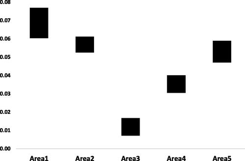
Our first hypothesis addresses whether the green affect varies by neighborhood. To test we ran the Full Model with each neighborhood interacted with the Green indicator to determine if there is a neighborhood green effect. Table 5 Panel B presents the regression results for these results. The Green premium is highest in the lowest value quintile (Area1) at almost 7%. The effect is not monotonic by value quintile. The rank order is; Area1 (6.9%), Area2 (5.7%), Area5 (5.3%), Area4 (3.5%), Area3 (1.2%). Examining the Confidence Intervals, we see that Area1 and Area2 are not statistically different and Area 2 and Area 5 are not statistically different. Area3 and Area4 are statistically different than the other Areas. To visualize the area effect, Figure 2 plots the confidence intervals by Area. Overall we can conclude that the green effect is highest in Area1, Area2, and Area5 and weaker in Area4 and weakest in Area3. If graphed, the coefficients show a U shape with lower values in the middling value quintiles. We reject our null hypothesis that there is no difference in Green premium by Area as there are non-overlapping confidence intervals as illustrated on Figure 2.

Figure 2. 95% Confidence Intervals for Green Premium by Area from Table 5 Panel B.

Our second hypothesis regards whether the green premium depends on homestead status. We interact the Green indicator with Homestead to create two variables to capture green effect by homestead status. The results, presented in Table 5 Panel C show a show that Non-Homestead homes have a much higher Green premium, 6.4%, while Green Homesteads show the lower 2.8% figure. Examining the confidence intervals shows this is a statistically significant difference which leads us to reject our null hypothesis that there is no difference by ownership status. We can only conjecture the reason for this strong result. Sellers of Non-Homestead properties may choose to distinguish their properties versus other Non-Homestead properties through their green investment, knowing green is less common in Non-Homestead properties.

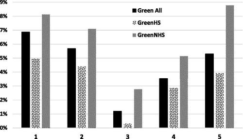
A logical extension to the area and homestead effect is to see whether the homestead effect has a similar affect across areas. For this we interact Homestead, Area, and Green to split the green indicator into 10 categories. We add control variables of homestead by area to better evaluate the green effect by area by homestead. Table 5 Panel D presents the results. Turning first to Area1, we find Non-Homesteads have a higher green coefficient (8.1%) than for Homesteads (5.0%). This result confirms the large green premium for Area1 and that Non-Homesteads have the larger premium. The confidence intervals for these estimates do not overlap demonstrating a statistically significant difference by homestead status. Moving to Area2 we find a premium of 7.1% for Non-Homestead and 4.4% for Homesteads. Once again the confidence intervals do not overlap showing there is a statistically significant green premium for Area2 by homestead status. For Area3, Non-Homesteads show a 2.8% Green premium, while the premium for Homesteads at 0.3% is not statistically different from zero. Their confidence intervals do not overlap. This is the only disaggregation thus far that finds no green premium. For Area4 and Area5 the results tell the same story that Non-Homesteads have a statistically larger Green premium than Homesteads. To visualize these results, Figure 3 plots the Green Premiums by area for all data, and disaggregated by Homestead status. The U shape is observed for all specifications across area.

Figure 3. Green Premium by Area by Homestead Status. Regression Coefficients from Table 5 Panel B and Panel D.

Our third hypothesis was to examine whether the Green premium was constant over time. One reason we do so is that market conditions may have changed over the period, or consumer demand for Green attributes may have changed. To demonstrate the change in market conditions over time, Figure 4 plots the monthly indicator variables that are not reported in Table 5 Panel A. The results reflect the relatively mild Texas effect of the great recession followed by robust recovery beginning in 2013 and continuing through the remainder of the data period. To evaluate a time trend in Green valuation, we ran a series of three regressions, for each of our eleven data years and report Green measures of interest in Table 6. The first regression uses a single Green indicator variable. Table 6, Panels A - K shows the results by year. In all cases the Green variable is statistically significant, though the estimated coefficient varies over time. From Table 6 we see the Green premium rose from less 3% in 2009 to about 5% for the 2011–2013 period, which roughly corresponds with the period where house prices did not rise. To quickly visualize this change over time, the 95% Confidence Intervals for the Green premium are plotted on Figure 5. Our point estimate for all years, 0.042, would pass through all of these confidence intervals, except for 2009 when it would be above the confidence interval, and for 2012 where it would be below the confidence interval. If we consider the confidence interval for all years combined of 0.039–0.045 we note it would touch the annual confidence intervals for all years except for 2009. So we must accept the Hypothesis 3 in that there is not a statistically significant time trend after 2009. For the years after 2014 the Green Premium remained about 4% and the confidence interval is quite stable through the beginning of 2019, where our data ends.

Figure 4. Monthly Indicator Variables for Regression Model reported in Table 5.

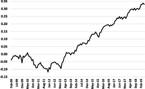
Figure 5. Confidence Intervals for Green Premium by Year. Confidence Interval Regression Results from Table 6, Panels A–K.

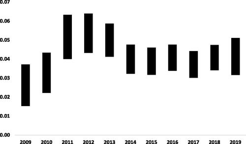
Table 6. Ordinary least squares regression results summary for full model by year.

	ParamEst	StdErr	t-val	Pval	VIF	95% Confidence	AdjR^2
Panel A: Year = 2009. N=8102
Green	0.026	0.006	4.68	<.0001	1.102	0.015–0.037	0.847
GreenArea1	0.067	0.021	3.12	0.002	1.142	0.025–0.109	0.847
GreenArea2	0.016	0.012	1.37	0.169	1.164	−0.007–0.039
GreenArea3	0.023	0.010	2.41	0.016	1.176	0.004–0.042
GreenArea4	0.003	0.010	0.33	0.745	1.249	−0.017–0.024
GreenArea5	0.066	0.013	5.22	<.0001	1.226	0.041–0.091
GreenHomeStd	0.016	0.007	2.40	0.017	1.222	0.003–0.029	0.847
GreenNotHomeStd	0.050	0.010	5.03	<.0001	1.155	0.031–0.070
Homestead	0.046	0.006	7.88	<.0001	1.564	0.034–0.057
Panel B: Year = 2010. N = 8129
Green	0.033	0.005	6.08	<.0001	1.150	0.022–0.043	0.863
GreenArea1	0.059	0.019	3.03	0.002	1.186	0.021–0.097	0.864
GreenArea2	0.042	0.010	4.22	<.0001	1.323	0.023–0.062
GreenArea3	0.030	0.011	2.85	0.004	1.371	0.009–0.051
GreenArea4	−0.002	0.009	−0.24	0.812	1.426	−0.021–0.016
GreenArea5	0.073	0.012	5.95	<.0001	1.399	0.049–0.097
GreenHomeStd	0.013	0.006	2.08	0.037	1.338	0.001–0.026	0.864
GreenNotHomeStd	0.074	0.009	8.06	<.0001	1.244	0.056–0.092
Homestead	0.046	0.006	7.27	<.0001	1.737	0.033–0.058
Panel C: Year = 2011. N = 9,247
Green	0.052	0.006	8.72	<.0001	1.185	0.040–0.063	0.860
GreenArea1	0.138	0.019	7.31	<.0001	1.152	0.101–0.175	0.860
GreenArea2	0.063	0.012	5.47	<.0001	1.348	0.041–0.086
GreenArea3	0.039	0.011	3.41	0.001	1.404	0.017–0.061
GreenArea4	0.045	0.011	3.91	<.0001	1.590	0.022–0.067
GreenArea5	0.022	0.013	1.71	0.087	1.649	−0.003–0.047
GreenHomeStd	0.026	0.007	3.62	0.000	1.404	0.012–0.040	0.860
GreenNotHomeStd	0.098	0.010	10.28	<.0001	1.240	0.079–0.117
Homestead	0.062	0.007	9.21	<.0001	1.724	0.049–0.075
Panel D: Year = 2012. N = 11,541
Green	0.054	0.005	10.15	<.0001	1.198	0.043–0.064	0.856
GreenArea1	0.099	0.013	7.77	<.0001	1.137	0.074–0.124	0.857
GreenArea2	0.078	0.011	7.26	<.0001	1.298	0.057–0.099
GreenArea3	0.032	0.010	3.30	0.001	1.389	0.013–0.051
GreenArea4	0.034	0.009	3.63	0.000	1.483	0.016–0.053
GreenArea5	0.046	0.012	3.95	<.0001	1.598	0.023–0.068
GreenHomeStd	0.035	0.006	5.40	<.0001	1.460	0.022–0.047	0.857
GreenNotHomeStd	0.088	0.009	10.33	<.0001	1.265	0.071–0.105
Homestead	0.050	0.006	8.06	<.0001	1.783	0.038–0.062
Panel E: Year = 2013. N = 14,093
Green	0.050	0.004	11.19	<.0001	1.187	0.041–0.059	0.857
GreenArea1	0.126	0.013	9.75	<.0001	1.195	0.101–0.151	0.857
GreenArea2	0.045	0.008	5.75	<.0001	1.343	0.029–0.060
GreenArea3	0.029	0.008	3.44	0.001	1.319	0.013–0.046
GreenArea4	0.039	0.008	4.92	<.0001	1.522	0.024–0.055
GreenArea5	0.055	0.010	5.48	<.0001	1.567	0.036–0.075
GreenHomeStd	0.030	0.006	5.46	<.0001	1.476	0.019–0.041	0.857
GreenNotHomeStd	0.083	0.007	11.85	<.0001	1.307	0.069–0.097
Homestead	0.062	0.005	11.50	<.0001	1.834	0.052–0.073
Panel F: Year = 2014. N = 15,357
Green	0.040	0.004	10.20	<.0001	1.157	0.032–0.048	0.859
GreenArea1	0.094	0.014	6.84	<.0001	1.143	0.067–0.121	0.859
GreenArea2	0.048	0.006	7.83	<.0001	1.305	0.036–0.061
GreenArea3	0.004	0.007	0.54	0.586	1.276	−0.010–0.018
GreenArea4	0.036	0.007	4.86	<.0001	1.381	0.021–0.050
GreenArea5	0.060	0.009	6.46	<.0001	1.539	0.042–0.078
GreenHomeStd	0.025	0.005	4.98	<.0001	1.457	0.015–0.034	0.859
GreenNotHomeStd	0.063	0.006	10.50	<.0001	1.300	0.051–0.075
Homestead	0.045	0.005	9.52	<.0001	1.821	0.036–0.055
Panel G: Year = 2015. N = 16,984
Green	0.039	0.004	10.74	<.0001	1.158	0.032–0.046	0.852
GreenArea1	0.065	0.010	6.53	<.0001	1.092	0.046–0.085	0.852
GreenArea2	0.062	0.006	9.98	<.0001	1.290	0.050–0.074
GreenArea3	0.007	0.007	1.09	0.275	1.348	−0.006–0.020
GreenArea4	0.052	0.007	7.15	<.0001	1.558	0.038–0.067
GreenArea5	0.015	0.008	1.84	0.066	1.831	−0.001–0.032
GreenHomeStd	0.028	0.005	6.05	<.0001	1.455	0.019–0.036	0.852
GreenNotHomeStd	0.056	0.006	10.10	<.0001	1.333	0.045–0.067
Homestead	0.034	0.004	7.73	<.0001	1.826	0.026–0.043
Panel H: Year = 2016. N = 17,716
Green	0.041	0.004	11.61	<.0001	1.155	0.034–0.048	0.845
GreenArea1	0.022	0.014	1.54	0.124	1.068	−0.006–0.049	0.845
GreenArea2	0.069	0.006	12.20	<.0001	1.292	0.058–0.080
GreenArea3	0.012	0.007	1.69	0.092	1.349	−0.002–0.026
GreenArea4	0.036	0.007	5.04	<.0001	1.656	0.022–0.050
GreenArea5	0.031	0.008	3.77	0.000	1.881	0.015–0.047
GreenHomeStd	0.031	0.004	6.90	<.0001	1.431	0.022–0.039	0.845
GreenNotHomeStd	0.056	0.005	10.42	<.0001	1.295	0.045–0.066
Homestead	0.035	0.004	8.31	<.0001	1.751	0.026–0.043
Panel I: Year = 2017. N = 17,000
Green	0.037	0.004	10.38	<.0001	1.170	0.030–0.044	0.834
GreenArea1	0.047	0.013	3.67	0.000	1.097	0.022–0.072	0.835
GreenArea2	0.048	0.005	8.92	<.0001	1.228	0.037–0.058
GreenArea3	−0.016	0.007	−2.40	0.016	1.240	−0.028 to −0.003
GreenArea4	0.058	0.007	8.45	<.0001	1.370	0.044–0.071
GreenArea5	0.062	0.009	6.96	<.0001	1.566	0.045–0.080
GreenHomeStd	0.030	0.004	6.61	<.0001	1.419	0.021–0.038	0.834
GreenNotHomeStd	0.049	0.006	8.90	<.0001	1.280	0.039–0.060
Homestead	0.042	0.004	10.12	<.0001	1.718	0.034–0.050
Panel J: Year = 2018. N = 19,192
Green	0.041	0.003	12.07	<.0001	1.170	0.034–0.047	0.827
GreenArea1	0.052	0.011	4.51	<.0001	1.097	0.029–0.074	0.827
GreenArea2	0.052	0.006	9.35	<.0001	1.255	0.041–0.062
GreenArea3	0.018	0.006	2.85	0.004	1.289	0.005–0.030
GreenArea4	0.026	0.006	4.19	<.0001	1.399	0.014–0.038
GreenArea5	0.071	0.008	9.18	<.0001	1.461	0.056–0.086
GreenHomeStd	0.030	0.004	7.20	<.0001	1.411	0.022–0.039	0.827
GreenNotHomeStd	0.057	0.005	10.95	<.0001	1.290	0.047–0.067
Homestead	0.031	0.004	7.97	<.0001	1.700	0.023–0.039
Panel K: Year = 2019 (Partial Year). N = 8,622
Green	0.041	0.005	8.36	<.0001	1.202	0.032–0.051	0.836
GreenArea1	0.073	0.017	4.27	<.0001	1.088	0.040–0.107	0.837
GreenArea2	0.044	0.008	5.80	<.0001	1.206	0.029–0.059
GreenArea3	0.008	0.010	0.83	0.407	1.227	−0.011–0.027
GreenArea4	0.028	0.008	3.40	0.001	1.471	0.012–0.044
GreenArea5	0.113	0.013	8.69	<.0001	1.358	0.087–0.138
GreenHomeStd	0.027	0.007	4.12	<.0001	1.500	0.014–0.040	0.837
GreenNotHomeStd	0.058	0.007	8.29	<.0001	1.271	0.044–0.072
Homestead	0.027	0.006	4.72	<.0001	1.770	0.016–0.038

Dependent Variable Log of Sale Price. Only covariates of interest displayed.

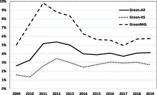
Figure 6, in addition to the point estimate for Green premium each year, also plots the results interacting Green with Homestead to determine whether the homestead effect is similar over time. This figure plots the GreenHomeStd and GreenNotHomeStd regression coefficients presented in Table 6, Panels A–K. The trend result is the same each year—Non-Homesteads have a higher Green Premium. Examining the confidence intervals by year, we find this difference is statistically significant in every year.

Figure 6. Green Premium by Year by Homestead Status. Regression Coefficients from Table 6, Panels A–K.

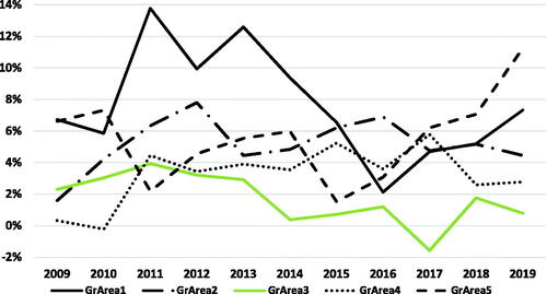
Finally, we address whether the Green premium difference by Area remain constant over time. The regression coefficients are presented in Table 6 Panels A–K. There are numerous regression coefficients presented in this table so we plot the coefficients to more easily assess their stability over time. Figure 7 presents this result. A cursory look at Figure 7 shows the Green by Area affect does change over time as the coefficients do not rise and fall in unison over time. Some outcomes can be gleaned from studying the plot and the table. Area1 showed the highest Green Premium for the combined data. Disaggregating it by year shows that there were 5 of the years where its premium was highest (2011, 2012, 2013, 2014, 2015), but only 2 years where it was statistically higher (2011, 2013) than all other Areas. Area3, which showed the lowest Green premium for the entire data set showed the lowest Green premiums from 2012 through the end of the data, but this result was not statistically different from other Areas. With the exception of 2018, it did not show a statistically positive coefficient after 2013. And, for 2017 it presented the only statistically negative coefficient in our analysis. Area4, which showed the second smallest green premium using the entire data, shows a coefficient not statistically different from zero for the first two years, and then seems to settle to about 4%. Overall there is substantial variation in the Green premium by Area result when disaggregated by year.

Figure 7. Green Premium by Year by Area. Regression Coefficients from Table 6, Panels A–K.

Conclusions

Houses with Green characteristics include energy and water savings, enhanced comfort, and potentially increase an owner’s sense of environmental responsibility—all of which should add value to a home. The analysis presented here measures a statistically significant increase in the sale price for properties with Green characteristics. For resale properties, with just over a decade worth of data, we find Green property sells at a 4.2% premium to otherwise identical properties.

Our goal in this paper was to use our extensive database to more deeply probe the value of Green. In particular, we address the Green premium by Area (approximate neighborhood value quintiles), homestead status, and time trend. When we disaggregate by Area, we find that the lowest value neighborhoods showed the greatest value premium from Green (almost 7%), and the median value neighborhoods provided the lowest premium (about 1.2%). Other neighborhoods provide a Green premium in the 3.5–5.7% range. When we disaggregate the result between Homestead and Non-Homestead, we find that Non-Homestead homes have a larger Green premium of 6.4% versus the 2.8% Green premium of Homestead homes. When we disaggregate the Green premium by Area and Homestead, the estimated Green Premium for Homestead homes in the middle value neighborhoods is not statistically different than zero.

We find that at the beginning of our data period (2009) the Green premium was 2.6%. It rose as high as 5.4% in 2012 and then settled on a value of about 4% from 2014 through the end of our data period. While the point estimates varied by year, the confidence intervals for most years overlapped so we cannot reject the null hypothesis that the Green premium was stable after 2009. When we evaluated the Green premium by year for Homestead and Non-Homestead homes, the Non-Homestead homes showed a statistically significant higher premium over Homestead homes in every year. When we examined the Area effect by year, we found the results were unstable on a year to year basis. Overall, we find a significant and enduring Green premium in resale residential real estate that we estimated at 4.2% of sales price over our entire data.

While this paper has extended the literature on the value of green in residential real estate, it has limitations. The data is from South Texas so the results may be more applicable to warmer climates than colder ones. The novel analysis here, including effect of value quintiles and ownership status, would benefit from confirmation in other locations and datasets. This paper notes how the model specification and depth of data affects the magnitude of the measured green effect. Should covariates that were unavailable in our data be correlated with the green variable it is possible that our green measures lack precision. The Variance Inflation Factors for our green estimates are all below 2.5 which indicates that collinearity with our covariates are not unduly affecting our estimated green measures.

Notes

1 Texas Comptroller of Public Accounts Publication #96-1740 February 2018.

2 For some high-end properties, a homeowner, for privacy reasons, could chose to the hold the home in an entity that does not qualify for homestead. In such cases presumably the owner believes that privacy is more valuable than the property tax savings and other protections.

References

- Adomatis, S. K. (2010). Valuing high performance houses. The Appraisal Journal, 78, 195–201.
- Adomatis, S. K. (2012). Describing the green house made easy. The Appraisal Journal, 80 (Winter), 21–29.
- Aroul, R. R., & Hansz, J. A. (2011). The role of dual-pane windows and improvement age explaining residential property values. Journal of Sustainable Real Estate, 3(1), 142–161. https://doi.org/https://doi.org/10.1080/10835547.2011.12091822
- Aroul, R. R., & Hansz, J. A. (2012). The value of “green”: Evidence from the first mandatory residential green building program. Journal of Real Estate Research, 34(1), 27. 49. https://doi.org/https://doi.org/10.1080/10835547.2012.12091327
- Aroul, R. R., & Rodriguez, M. (2017). The increasing value of green for residential real estate. Journal of Sustainable Real Estate, 9(1), 112–130. https://doi.org/https://doi.org/10.1080/10835547.2017.12091894
- Bloom, B. C., Nobe, M. C., & Nobe, M. D. (2011). Valuing green home designs: A study of ENERGY STAR® homes. Journal of Sustainable Real Estate, 3(1), 109–126. https://doi.org/https://doi.org/10.1080/10835547.2011.12091818
- Butler, R. V. (1982). The specification of hedonic indexes for urban housing. Land Economics, 58, 94–108. https://doi.org/https://doi.org/10.2307/3146079
- Cadena, A., & Thomson, T. A. (2015). An empirical assessment of the value of green in residential real estate. The Appraisal Journal, Winter, 83, 32–40.
- Chin, T. L., & Chau, K. W. (2003). A critical review of literature on the hedonic price model. International Journal for Housing and Its Applications, 27(2), 145–165.
- Ciochetti, B. A., & McGowan, M. D. (2010). Energy efficiency improvements: Do they pay? Journal of Sustainable Real Estate, 2(1), 305–333. https://doi.org/https://doi.org/10.1080/10835547.2010.12091807
- Dastrup, S. R., Zivin, D. C., & Kahn, M. E. (2012). Understanding the solar home price premium: Electricity generation and “green” social status. European Economic Review, 56(5), 961–973. https://doi.org/https://doi.org/10.1016/j.euroecorev.2012.02.006
- Goodwin, K. R. (2011). The demand for green amenities. Journal of Sustainable Real Estate, 3(1), 27–41. https://doi.org/https://doi.org/10.1080/10835547.2011.12091827
- Herath, S. K., & Maier, G. (2010). The hedonic price method in real estate and housing market research. A reviewq of the literature. In Institute for regional development and environment (pp. 1–21). University of Economics and Business.
- Levinson, A. (2016). How much energy do building energy codes save? Evidence from california houses. American Economic Review, 106(10), 2867–2894. https://doi.org/https://doi.org/10.1257/aer.20150102
- Ma, A., & Narwold, A. (2019). Which way is up? Orientation and residential property values. Journal of Sustainable Real Estate, 11(1), 40–59. https://doi.org/https://doi.org/10.22300/1949-8276.11.1.40
- Malpezzi, S. (2003). Hedonic pricing models: A selective and applied review. In T. O’Sullivan, K. Gibb, & M. A. Malden (Ed.), Housing economics and public policy (pp. 7–89). Blackwell Science.
- Pride, D. J., Little, J. M., & Mueller-Stoffels, M. (2017). The value of energy efficiency in the anchorage residential property market. Journal of Sustainable Real Estate, 9(1), 172–194. https://doi.org/https://doi.org/10.1080/10835547.2017.12091897
- Rosen, S. (1974). Hedonic prices and implicit markets: Product differentiation in pure competition. Journal of Political Economy, 82(1), 34–55. https://doi.org/https://doi.org/10.1086/260169
- Rosen, S. (2002). Markets and diversity. American Economic Review, 92(1), 1–15. https://doi.org/https://doi.org/10.1257/000282802760015577
- Sewalk, S., & Throupe, R. (2014). The fesibility of reducing greenhouse gas emissions in residential buildings. Journal of Sustainable Real Estate, 5(1), 35–65.