Piping erosion safety assessment of flood defences founded over sewer pipes

Abstract

Piping erosion is one of the major causes of failure of flood defences. The occurrence of this failure mechanism is difficult to predict and it can be triggered during a flood event. The inclusion of hard structures under flood defences will change the probability of occurrence of this erosion process. The present study aimed at understanding the effect of an embedded sewer pipe under the flood defence foundation in its safety assessment for piping erosion failure. This was done by setting a probabilistic analysis framework based on emulation of finite element models of porous media flow and the fictitious permeability approach. The effects of size and location of the sewer pipe were evaluated via a deterministic safety factor approach. Afterwards, emulators of the most safe and unsafe models were trained and used for probabilistic assessments. The results showed that the embedment of a sewer pipe in the flood defence foundation has a significant effect on its safety. The magnitude of the effect is highly dependent on the size and location of the sewer pipe. Furthermore, the foundation permeability uncertainty shows a conditional effect with respect to the sewer pipe size and location.

Keywords:

• piping erosion
• flood defence
• failure
• sewer pipe
• artificial neural networks
• emulators

1. Introduction

Piping erosion is a deterioration process that threatens flood defences by compromising their structural stability during a flood event. This failure consists in the progression of erosion ‘channels’ underneath the flood defence granular foundation due to water movement. It is originated from the head difference between the water body and the protected side when the water level rises. Recently, large interest has emerged in the modelling, prediction and uncertainty assessment of this failure mechanism. More specifically, in the probabilistic estimation of the occurrence of this kind of failure (Hoffmans, 2014). The inclusion of an embedded structure located underneath the flood defence will change the groundwater flow patterns and consequently will have an effect in the piping erosion failure prediction and uncertainty as well. Flood risk managers and urban planners are inclining towards solutions such as multifunctional flood defences (Van Loon-Steensma & Vellinga, 2014; Van Veelen, Voorendt, & Van der Zwet, 2015) given climate change and demographic explosion in urban areas. If so, the combination of flood defence strategies and additional embedded infrastructure such as sewer pipes will become an option instead of an exception.

Probabilistic assessment of structural deterioration processes (failure mechanisms) consists in the propagation of variable uncertainties through a model which is later used to assess the probability of occurrence of an event. For the particular case of piping erosion and sewer pipes, the model used for the uncertainty propagation should be capable of predicting whether the piping erosion progresses or not. At the same time, it should include the effects of the additional structure on the groundwater flow.

The most relevant modelling approaches for piping erosion were grouped into three categories based on the type of representation of the process (Wang, Fu, Jie, Dong, & Hu, 2014). The first category is composed of models which represent the piping zone as a less impermeable soil. They consider the pore pressure distribution in the whole foundation during the modelling process. The application of this kind of models has been found in three different piping erosion studies (Bersan, Jommi, Koelewijn, & Simonini, 2013; Jianhua, 1998; Vandenboer, Van Beek, & Bezuijen, 2014). The second category consists of models that are capable of representing the mixture of water and soil flow inside the progressing channel. This is done by combining the numerical solution of the Darcy (fully saturated) or Darcy–Brinkman’s (partially saturated) equations for the porous media domain with the Navier–Stokes equations for the purely water domain. At the same time, particles are modelled individually based on a particle tracing trajectory numerical solution. Such methods are quite detailed and allow to describe the erosion progression in time, but are computationally demanding given the individual particle modelling. Examples of these models (El Shamy & Aydin, 2008; Lominé, Scholtès, Sibille, & Poullain, 2013) show promising results as well. The third category includes the models (Lachouette, Golay, & Bonelli, 2008; Sellmeijer & Koenders, 1991; Zhou, Jie, & Li, 2012) where soils are divided into phases with different erosion models which are governed by different physic laws. The numerical model used in the present study for uncertainty propagation corresponds to the first category.

The uncertainty in the water levels and the soil characteristic values will highly influence the safety assessment of piping failure (Sellmeijer, López de la Cruz, van Beek, & Knoeff, 2011). For the particular case in which a sewer pipe is embedded in the foundation, the combined effects from the earlier mentioned uncertainties plus the ‘atypical’ behaviour in the groundwater flow due to the inclusion of the hard structure will make safety assessment even less accurate. Then, the probabilistic methods become a more suitable type of assessment as they can include the most relevant uncertainties for the system. To our knowledge, there is no available literature that presents the probabilistic effect on piping erosion originated from the presence of hard structures embedded in the foundation of the flood defence. The only study found which included structural embedment (Wang et al., 2014) recreated the progression of piping erosion in time with a cut-off wall under a flood defence. The drawback of this method is its demanding numerical solution which requires an iterative process that makes it computationally expensive and unreliable for probabilistic safety assessments. Note that the propagation of the variables uncertainty implies large amount of simulations which in some cases may be computationally unfeasible.

In reliability science, it is common practice to use model simplifications, which only determines the state of the system based on the most relevant ‘state variables’ instead of modelling the physical process. These models are represented in the form of ‘limit state functions’. These functions represent the difference between the resistance (R) of the structure against a failure mechanism and its solicitation load (S). These types of models are more suitable for probabilistic safety assessment as they are easier to evaluate (reduced computational burden) and can be built based on more complex numerical solutions if required. In the case of piping erosion failure, several notable examples of limit state equations are commonly used for either levee or large dam safety assessment. (Bligh, 1910; Lane, 1935; Ojha, Singh, & Adrian, 2008; Sellmeijer et al., 2011; Terzaghi, Peck, and Mesri (1996)). These models do not allow to explicitly include the effects of embedded structures in the groundwater flow. Hence, the uncertainty of their application in safety assessments increases when embedded structures are present underneath.

The present study aimed at developing a methodology that allows to understand and quantify the effect on the safety assessment of piping erosion derived from placing a hard structure underneath a flood defence. As a realistic example, we use the embedment of a sewer pipe inside a granular foundation of a dike. The models used in the present study for performing the different assessments are based on the results obtained from the IJkdijk real-scale experiment for piping erosion (Koelewijn et al., 2014). In order to do that, three main research questions were formulated for assessing the safety of the flood defence:

(1)	How can we model the process of piping erosion while including an embedded sewer pipe and the soil uncertainties at the same time ?
(2)	What are the effects of the sewer pipe characteristics such as size and location in the flood defence safety ?
(3)	What are the effects of the water loads and soil uncertainty in the safety assessment of a flood defence with a sewer pipe embedded in its foundation?

The present paper explains the methodology used for solving these three research questions. First, the IJkdijk experiment is explained in Section 2. Afterwards, the steps of the methodology used for building the FEM models for the deterministic and probabilistic assessments are explained in Section 3. This part allows to solve the research question 1. The data and stochastic distributions (parametric uncertainties) used for building the model emulators and performing both (deterministic and probabilistic) safety assessments are presented in Section 4. The results of both safety assessments are presented in Section 5 which are used to solve the second and third research questions. Finally, the conclusions of the study are compiled in Section 6.

2. Ijkdijk full-scale experiment

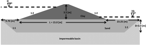
Full-scale experiments for levee failures were performed as part of the ‘IJkdijk’ Dutch research project (initiated in the year 2005). The project (Koelewijn et al., 2014; Van Beek, Knoeff, & Sellmeijer, 2011) aimed at testing monitoring techniques and improving the knowledge on geotechnical failure mechanisms of flood defences in real-scale structures. For the case of piping erosion, the experiment consisted in monitoring the erosion process inside the foundation of a real-scale flood defence due to an incremental water load, until achieving the complete failure process. Four tests were performed in flood defences built with the exact same cross section as the one shown in Figure 1. Each of the four experiments was composed of an impermeable levee founded in a different type of sand.

Figure 1. IJkdijk cross section for piping erosion test (not in scale).

For the present study, the experiment number 3 performed in 2009 was selected as there was no clogging of the erosion channel during the test. The measured characteristics and results from the experiment (Koelewijn et al., 2014) are shown in Table 1.

Table 1. IJkdijk experiment 3 parameters and results.

Parameter	Value	Unit
Aquifer permeability (k)	1.07e−11	(m^2)
Representative grain diameter (d70)	180.0	(μm)
Potential seepage length (L)	15.0	(m)
Aquifer depth thickness (D)	3.0	(m)
Critical head difference to failure (Hc)	2.1	(m)

3. Method

In short the method consists in building and calibrating a detailed finite element model (FEM) of a conventional flood defence based on the measured conditions from the ‘IJkdijk’ piping real-scale experiment presented in Section 2. The grain equilibrium concept for piping erosion (Sellmeijer, 1988) was used for building all FEM models built in this study. To simplify the numerical solution, a fictitious permeability equivalence was implemented (Bersan et al., 2013). The most important aspects for calibrating this model are the erosion channel average size and shape. To our knowledge there is no literature available for predefining these characteristics of the erosion channel in a model. Hence the first part of the study consisted in a sensitivity analysis of this parameter for determining the best choice based on the IJkdijk experimental results. After defining the size and shape of the erosion channel, the aquifer depth and permeability influence in the erosion capacity were also studied in this analysis. The rest of the parameters were available from the reports of the experiment. This calibration and validation procedure corresponds to the first part of the study.

The second part of the study consisted in modifying the initial model by including an embedded sewer pipe. This process is repeated several times for different sizes and locations of the embedded structure in order to assess its effect in the safety factor of the structure. This part corresponds to the ‘deterministic’ safety assessment of the structure.

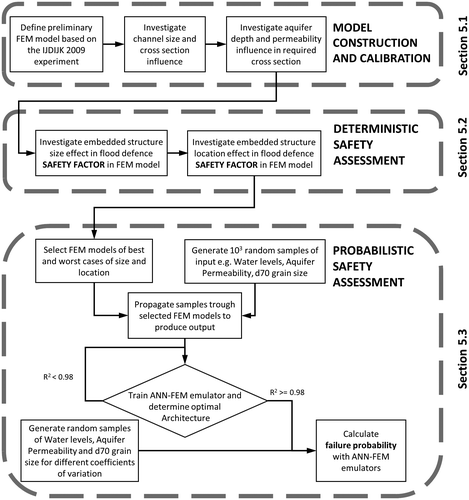
For the third part of the present study, the most safe and unsafe configurations found in the deterministic assessment are selected for further analysis. For each of these cases, an artificial neural network (ANN) emulator was built (referred as surrogate models in Chojaczyk, Teixeira, Neves, Cardoso, & Guedes Soares, 2015). This was done by generating training data from the original FEM models. These models were later used for failure probability estimation. This analysis corresponds to the probabilistic safety assessment. The order of the steps taken for each section is presented in the methodology flow chart of Figure 2.

Figure 2. Methodology flow chart.

3.1. Piping erosion model

The numerical solution for the present study corresponds to a multiphase piping erosion type of model. Two different configurations of FEM models were built for the present study for the safety assessment as presented in Figure 3.

Figure 3. IJkdijk cross section and boundary conditions of FEM models with and without embedded sewer pipe.

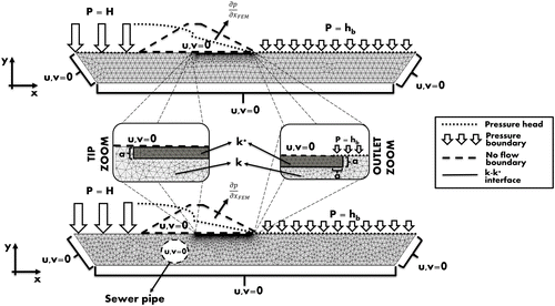
The first model corresponds to the case of a flood defence with no sewer pipe embedded in the foundation aquifer. The second model includes an embedded sewer pipe (a hollow circle boundary with no inflow or outflow in any direction) inside the foundation aquifer. Later the size and location of the sewer pipe is changed and a new model is produced. All models were built based on the ‘IJkdijk’ experimental flood defence dimensions presented in (Koelewijn et al., 2014). Both have the same external boundary condition definition. The boundaries with pressure distributions allow water inflow towards the porous media whereas the ones with null velocity component represent the absence of inflow as presented in Figure 3.

According to Sellmeijer’s conceptual model (Sellmeijer, 1988), the equilibrium condition of piping erosion is defined by the horizontal pressure gradient exerted inside the erosion channel and the rolling resistance of grains. This condition is represented by a two forces limit equilibrium assumption. According to experimental findings (Sellmeijer & Koenders, 1991), it is assumed that this equilibrium condition becomes critical once the erosion channel has progressed until approximately the midpoint of the flood defence. If the pressure gradient becomes larger than the rolling resistance at this particular point, the erosion progression will continue indistinctively from the loading conditions of the structure until the failure of the flood defence foundation. This condition is predefined in the FEM model by the inclusion of the erosion channel until the exact midpoint, as it can be observed in Figure 3. The thick dashed line represents the impermeable flood defence body.

3.1.1. Load term (S)

The pressure gradient inside the predefined erosion channel (Figure 3) is the only required output from the model for assessing the occurrence of the piping erosion failure. Both FEM models are solved for a steady state condition of the system. This choice is correct for systems where the ‘limit state’ condition does not include any time dependencies as the one presented in this study. Hence, the flow inside the porous media can be solved by the steady state Darcy’s law (Equation 1(1) ):(1)

The equation is used to estimate the flow velocity (u) of the water through the porous medium as a function of the soil permeability (k) and the hydraulic gradient (∇H). In terms of the flow inside the erosion channel, the Navier–Stokes equations would be the most correct approach. However, the solution of the combined equation system (Darcy and Navier–Stokes) becomes difficult as the boundary conditions of both models are dependent on each other. If so, the solution of the model becomes an iterative process until both boundary conditions are satisfied. This process is computationally demanding when a large number of simulations are required as in the case of probabilistic assessment.

The fictitious permeability method (also referred as continuum solution for fracture flow (Bear & Verruijt, 1987; Chen, Gunzburger, Hu, Wang, & Woodruff, 2012; Liedl, Sauter, Hückinghaus, Clemens, & Teutsch, 2003; Samardzioska & Popov, 2005)) allows to avoid the boundary iteration by assuming that the erosion channel is filled with a porous material of high permeability value (k^*). Hence all domains (aquifer and erosion channel) can be solved with Equation 1(1) only. A comparison study (Bersan et al., 2013) of piping modelling concluded that no major implications are derived from this assumption when compared to the complete solution of the Navier–Stokes and Darcy–Brinkman numerical solution for two and three dimensions. Similar approaches were used in the study (Wang et al., 2014; Zhou et al., 2012) that included the sheet pile effect. The simplification derived from the Darcy–Weisbach equation (Mott, Noor, & Aziz, 2006) for the head loss pressure gradient ) inside a closed conduit of hydraulic diameter (D_h) is presented in Equation 2(2) :(2)

In the present study, the resistance of flow assumed to be only significant in the x direction given the relation of height versus length of the erosion channel. Hence, the permeability coefficient inside the foundation is assumed to be the same in x and y directions. Based on the deduction presented in the work of Muzychka and Yovanovich (2009), The flow friction factor (f) can be written as a function of the Reynolds number (Re) and a β_fi factor which depends on the cross section shape (Equation 3(3) ):(3)

Additionally, the Reynolds number of a close conduit is expressed in terms of the hydraulic diameter and the fluid characteristics (density (ρ) and dynamic viscosity (μ)) as:(4)

When substituting Equations 3(3) and 4(4) in Equation 2(2) , the velocity (u) inside a pipe can be expressed in terms of Darcyan flow as:(5)

Assuming that the flow velocity and pressure gradients are equivalent inside a pipe filled with water that flows in a laminar regime, it can be concluded that the required fictitious permeability (k^*) in Equation 1(1) can be written as:(6)

The β_fi coefficient for fully laminar developed flow is dependent on the cross section shape (Muzychka & Yovanovich, 2009). Different coefficients are presented in Appendix A for each type of geometrical cross section. If a vertical segment was added to the erosion channel, the resistance in the y direction should also be included in the model (Wang et al., 2014).

The most relevant and updated piping erosion modelling literature (Bersan et al., 2013; Lachouette et al., 2008; Sellmeijer & Koenders, 1991; Van Esch, Sellmeijer, & Stolle, 2013; Vandenboer et al., 2014; Wang et al., 2014; Zhou et al., 2012) assumes a prior knowledge of the size and/or shape of the erosion channel. For the fictitious permeability solution, the channel geometry becomes great source of uncertainty as there is no literature that recommends how to predetermine it. Hence, five different cross section geometries presented in Appendix A were tested in different sizes, in order to calibrate the model and suggest a tentative choice for other modellers. Note that the calibration of this parameter also depends on the soil parameters which are assumed as the most relevant by Sellmeijer. Hence in this study, the size of the channel was denoted in terms of the variable n_g which allows to express the erosion channel in terms of the representative grain size (d₇₀) and the erosion channel height (a) included in Sellmeijer model.(7)

The findings and remarks about erosion channel height based on Sellmeijer model (Van Beek, Vandenboer, & Bezuijen, 2014; Van Esch et al., 2013) were also expressed in terms of n_g and were used for the validation of the present 2D modelling. The values of a and β_fi obtained for experimental conditions of the ‘IJkdijk’ (Koelewijn et al., 2014) were used for building the finite element models indistinct if they included the additional structure or not. Hence, the only difference is that the former ones represent the embedded structure as a closed boundary condition in which neither inflow nor outflow occurs (u,v = 0, figure 3).

3.1.2. Resistance term (R): two forces equilibrium

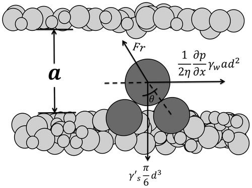
Once the pressures inside the aquifer and the erosion channel are known, it is required to check if the resultant inner pressure gradients are high enough so that the grains can be eroded. This can be estimated based on the equilibrium of forces acting on a single grain (Figure 4). The contact area of the grain is expressed as a function of the White’s (η = .25) sand packing coefficient (White, 1940) and the representative particle diameter (d).

Figure 4. Two forces grain equilibrium model inside the erosion channel.

Solving the system in equilibrium of forces (Van Esch et al., 2013), it is possible to conclude that:

(8)

In reality, the representative d₇₀ grain size can be correlated to the aquifer permeability variable included in the load term (S). This correlation can be induced during the sampling process of both d₇₀ and k. Despite the fact that this correlation effect can have a significant impact in the probabilistic assessment of piping erosion (Aguilar-López, Warmink, Schielen, & Hulscher, 2016), it is out of the scope of this study and therefore it is not considered.

3.2. Sellmeijer limit state recalibrated equation

Due to the complexity of the numerical model, Sellmeijer developed a complementary limit state equation (Sellmeijer & Koenders, 1991) from curve fitting for design purposes of conventional flood defences. In 2011, this equation was modified and calibrated (Sellmeijer et al., 2011) based on the two forces approach explained previously in Section 3.1. The equation was recalibrated again with additional experimental correction factors via multivariate analysis as presented by Van Beek in (Van Beek, 2015). These results differ significantly from the theoretical modelling results for extreme values. Hence, the 2011 equation (Sellmeijer et al., 2011) is selected for validation of the obtained failure probabilities from the emulators as it is more reliable for stochastic modelling. The equation is presented in Appendix B.

3.3. Deterministic safety assessment

The main output of the FEM model is the resultant pressure gradient inside the erosion channel for a specific set of boundary conditions and soil characteristics (e.g. permeability, aquifer depth, specific weight, etc.). This pressure gradient represents the solicitation (S) or ‘load’ of the system. The resistance (R) of grains to roll can be also expressed as a critical pressure gradient as explained in Section 3.1. In reliability studies, the ratio between the resistance term (R) and the load (S) is commonly referred as the safety factor (Elishakoff, 2012). For the present study, the safety factor (SF) for piping erosion is defined as:(9)

The exact definition of the safety factor is extensively discussed (Elishakoff, 2012) for the cases where (R) and (S) are defined as deterministic, probabilistic or a combination of both. For the second part of the study, both terms are assumed as deterministic. The resistance term is defined by the critical pressure gradient which represents the threshold pressure value required for the grains to roll. This value is derived from the two forces limit state equilibrium concept (Section 3.1). The safe condition is defined by SF > 1 and conversely unsafe if SF ≤ 1.

3.4. Probabilistic safety assessment

When the model parameters are expressed as uncertainties in the form of random variables, their load (S) and resistance (R) can be expressed as uncertainties as well. This representation is more convenient for assessing the safety state of the structure in a probabilistic manner. However, the safety state is now defined by the safety margin instead of the safety factor. This notation form allows to include the cases where the solicitation is equal to zero. This kind of notation is referred to as limit state function and its general form is expressed as:(10)

In which X and Y are vectors of random variables used as inputs of R and S models in each model ith model run. In order to estimate P(Z < 0) from the resultant Z distribution, a large number of model runs are required in order to ensure that the extreme events located in the tail of the distribution are also generated. Normally these events correspond to the failure state. Such procedure becomes computationally unfeasible when FEM models are to be used for propagating uncertainties due to the computational burden. In those cases, first- and second-order reliability methods (FORM and SORM; Low, 2014) become a more attractive choice as they require a significantly lower number of models runs of the FEM’s when compared to a Monte Carlo reliability method. The problem with FORM and SORM methods is that prior knowledge of the failure functions is required in order to linearise them. This requirement makes both methods difficult to implement if no prior knowledge of the functions is available. This is the case for porous media flows with large heterogeneities. Therefore, an ANN emulation methodology (Chojaczyk et al., 2015) was implemented for replicating the FEM numerical solution for the probabilistic analysis. Emulating (metamodeling or also known as surrogate modelling) is a common practice in reliability studies where high precision approximations of an original model are required for calculating large amounts of simulations with low computational costs (Bucher & Most, 2008; Forrester, Sobester, & Keane, 2008; Li, Chen, Lu, & Zhou, 2011; Lü & Low, 2011; Schoefs, Le, & Lanata, 2013; Shamekhi & Tannant, 2015; Zhang, Chen, Huang, & Luo, 2015). Such models consist in propagating different input combinations through a complex model such as an FEM to produce a significant amount of input-output data-sets. These are later used for building an approximation of the original model. The multilayer perceptron ANN algorithm was selected as it has proven to be successful in approximating non-linear behaviour of different type of structures (Cho, 2009; Chojaczyk et al., 2015; Kaunda, 2015; Kingston, Rajabalinejad, Gouldby, & Van Gelder, 2011; Yazdi & Salehi Neyshabouri, 2014). For the case of piping erosion based on Sellmeijer conceptual model, a robust network was trained (Sellmeijer, 2006) for cases where no additional structure was embedded. This method proved to be sufficiently accurate for predicting the critical head, but the training set was quite large (16807 samples) and based on the Mseep software numerical solution (Sellmeijer, 1988) which requires an iterative method for solving the boundary conditions as mentioned previously. The fictitious permeability method presented in the present study allows to implement the method in any FEM groundwater software that allows fine meshing generation inside the potential erosion channel. For the present study, the emulator (denoted by Ω) is defined as an approximation function of the original FEM model as follows:(11)

where H corresponds to the water level in the river side of the flood defence, h_b corresponds to the water level in the hinterside and k corresponds to the permeability value of the aquifer foundation. These two inputs were selected as the only stochastic parameters for the emulators as they account for most of the model variability (Sellmeijer et al., 2011).

These inputs are also propagated as uncertainties in the original FEM model. After propagating the samples through the FEM and training the emulators, the limit state functions can be defined as:(12) (13)

Note that the FEM model calculates the pressure gradient as a function of the head difference whereas the emulator is trained based on the total water load height (H). The critical pressure gradient also has a stochastic nature as it is a function of the d₇₀ stochastic variable. Note that this function is independent of the Ω function.

4. Data

4.1. Stochastic distributions of input variables

For the probabilistic assessment, the parameters presented in Table 1 become stochastic random variables. Their statistical distributions and coefficient of variation (CV) were extracted from the study of Schweckendiek, Vrouwenvelder, and Calle (2014) as presented in Table 2. The IJkdijk experiment does not represent any specific site and therefore there were no hydraulic boundary conditions associated to this structure. The IJkdijk experiment has a 3.5 m height as shown in Figure 1. Based on the future safety standards of the Netherlands, the lowest safety value for this kind of structures correspond to a 100 years return period. In practice, it is recommended to have at least .5 m of freeboard for riverine dikes. Therefore, the boundary condition for the water levels (H) is fitted arbitrarily to a Gumbel distribution with two fitting parameters (a, b, Table 2) for a 100 years return period corresponding to a 3 m water level.

Table 2. Prior distributions of random variables for FEM models and Sellmeijer limit state equation.

Variable	Unit	Distributed	Mean	CV	λ
k	(m^2)	Log-normal	1.07e−11	1.0	1.5
d70	(μm)	Log-normal	180	.15	1.5
L	(m)	Constant	15	–	–
D	(m)	Constant	*	–	*
H	(m)	Gumbel	a = 1.569	b = .311	1.5
Additional parameters required for Sellmeijer 2011 (Appendix B)
η	(–)	Constant	.25	–	–
γsand	(kN/m^3)	Constant	26.5	–	–
γwater	(kN/m^3)	Constant	9.81	–	–
θ	(deg)	Constant	37	–	–
mp	(–)	Log-normal	1	.12	–
hb	(m)	Constant	.1	–	–
bimp	(m)	Constant	0	–	–

^* In order to study the influence of the aquifer depth, four different aquifer models were tested with depths of 3, 5, 8, 30 m.

4.2. FEM emulator training data-set

Ten thousand variable samples were generated randomly following the statistical distributions presented in Table 2. Afterwards, they were propagated through the original FEM. This number of samples ensures that the expected standard error in the Monte Carlo simulation remains close to 1%. Finally, input and output sets constitute the basis for training and validating the neural networks. It is possible that after training these models, the new generated samples used for the future probabilistic analysis are sampled outside the training data-set. If so, the emulators will have to extrapolate for those combinations of inputs and consequently large errors may be induced. To avoid this kind of errors, the initial training random samples were generated maintaining the mean value of the original models but increasing their ‘spreading’. In other words, the original CV from the distributions presented in Table 2 were modified. This was done by multiplying the CV values by an amplification factor (λ, Table 2) before generating the training data samples used as input in the FEMS. This ensures that the model is trained for values located further in the tail which reduce the chances of extrapolation.

5. Results and discussions

5.1. Optimal erosion channel shape and size

According to Sellmeijer conceptual model (Sellmeijer, 1988), the groundwater parameters that contribute most to the inflow of the erosion channel are the aquifer depth and the aquifer permeability. In that order of ideas, the erosion channel geometry and its inner pressure loss will also have a significant effect on the amount of inner inflow. For this reason, the influence in the progression capacity from these three parameters was tested for their implementation in the models used for the safety assessment.

5.1.1. Erosion channel cross section shape

The hydraulic gradients inside the erosion channel for the different cross section sizes were estimated as presented in Figure 5. The critical head value (H_c) obtained during the IJkdijk experiment (Table 1) was used for all models as a fixed boundary condition. The grain number coefficient n_g (Equation 7(7) ) allows to calculate both the exerted inner pressure gradient and the critical one (2 forces dashed line, Figure 5) in terms of the erosion channel height. The intersection between the two lines defines the maximum channel height threshold required for building sufficient pressure inside the channel to drag the representative sand particle.

Figure 5. Required erosion channel height (in terms of n_g), for different cross section geometries.

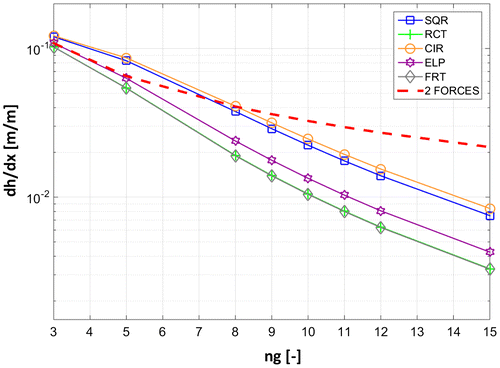
Channels with larger diameters will not generate sufficient inner pressure gradients for dragging the grains towards the outlet. For the case of the circular cross section, a n_g= 8.2 grains is obtained which is close to the 10 grain approximate size reported in the modelling study (Van Esch et al., 2013) and very close when compared to the one obtained in a latest experimental study (Van Beek et al., 2014).

Other cross section geometries such as the square and elliptical present lower thresholds whereas the rectangular and fracture ones present no eroding capacity at all for any given channel height. The results in terms of height of the erosion channel are consistent with the literature experimental findings. In the case of the width size, there is no agreement between the different authors (Bersan et al., 2013; Van Beek et al., 2011; Vandenboer et al., 2014; Wang et al., 2014; Zhou et al., 2012). For the present study, a single 2D erosion channel with constant circular cross section was assumed. The results from the study by Van Beek et al. (2014) showed that when the cross section size was represented as an average value for the whole length, the width/depth ratio tends to be closer to the unity for one of the experiments (width/depth = 3.5 mm/3.2 mm) and 2.5 times (width/depth = 8.4 mm/3.3 mm) for a second experiment. From the previous mentioned studies and the results presented in Figure 5, the fracture flow approach can be discarded for modelling piping erosion. Note that piping erosion is a three-dimensional process which includes an erratic meandering progression, multiple derivation of secondary channels and non-uniform cross section. Hence, the measured pressure loss inside the channel of an experimental set-up is greater than the one obtained in a two-dimensional model with a cross section that is significantly wider with respect to its depth. The fictitious permeability approach allows to compensate for this additional pressure loss by producing a narrower cross section with a width depth ratio closer to 1. This statement agrees with the results obtained for the circular and square sections of the present study. In addition, the results presented in Van Beek et al. (2014) for FEM modelling showed that an equivalent conductivity value of .5 m/s (the conductivity can be estimated as a function of the soil permeability and fluid properties as explained in the note of Appendix B) inside the erosion channel gave the best fit for representing the experimental data. For the present study, the resultant equivalent fictitious conductivity of the circular cross section with a height of 8.2 n_g is .49 m/s whereas for the square cross section is .54 m/s. Based on these results, a circular cross section with an n_g coefficient of 8.2 is chosen. All models are built with this same geometry except for the ones studied in Sections 5.3.4 and 5.3.5 where the n_g (channel height) was modified as a function of the aquifer depths given the results presented in Section 5.1.3. Nevertheless, the results show that a square section can be implemented as well.

5.1.2. Aquifer permeability effect on the cross section size

Several permeability values were tested between .01 and 100 times corresponding to highly impermeable and highly permeable soils (Bear & Verruijt, 1987). The permeability value of the aquifer foundation from the IJkdijk experiment corresponds to a fine sand of good permeability. Figure 6 shows that for very low permeability values (representative of very fine sands), the system will not be able to build a sufficiently high-pressure gradient inside the erosion channel so that the grain particle can be dragged.

Figure 6. Required erosion channel height (in terms of n_g), for different aquifer permeability (k) values.

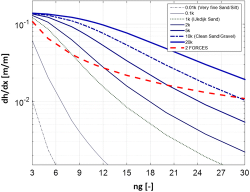
For the IJkdijk case (high permeability aquifers of clean sand) and larger d₇₀ grains (10 times k in Figure 6), the results agree with the reported experimental findings (Van Esch et al., 2013) which stated that values of n_g = 10 grains in experimental set-up and n_g = 30 grains in field surveys for coarser sands where observed. Based on these results it is concluded that the aquifer permeability has a very large influence in the eroding capacity and therefore it should be represented as a random variable instead of a calibration value for the probabilistic assessment.

5.1.3. Aquifer depth effect on the cross section size

Four different aquifer depths were tested (3, 5, 8 and 30 m). The results showed that from 3 to 8 m depth, the variation of the required erosion height fluctuated between 8 and 10 grains (Figure 7).

Figure 7. Required erosion channel height (in terms of n_g), for different aquifer depths.

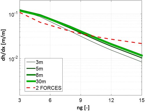
For thicker aquifers (D > 8 m), there is no additional depth-related effect observed as the pressure gradient lines are overlapping. Therefore, the range of variation of this parameter can be bounded. Hence, this characteristic was not represented as a stochastic parameter in the probabilistic safety assessment. Instead, several aquifer depths with their correspondent erosion channel height were tested.

5.2. Deterministic safety assessment for structural embedment

Three different commercial size sewer pipes were selected for this analysis. Diameters of .8, 1.0 and 1.2 m were selected assuming that such sizes will have a significant effect in the flow paths inside the aquifer. In terms of the sewer pipe position, eight locations in the horizontal direction and three in the vertical location were modelled. Their corresponding safety factor value was obtained based on Equation 9(9) . In Figure 8, the obtained safety factor values are written in the exact location corresponding to the centre of the assessed sewer pipe. For the most critical and favourable locations, the perimeter of the sewer pipe is plotted with a dashed line while preserving the scale. The erosion channel is represented by a thicker dashed line along the bottom of the flood defence.

Figure 8. Safety factor as a function of location for (a) 0.5 m diameter, (b) 0.8 m diameter, (c) 1.0 m diameter, (d) 1.2 m diameter.

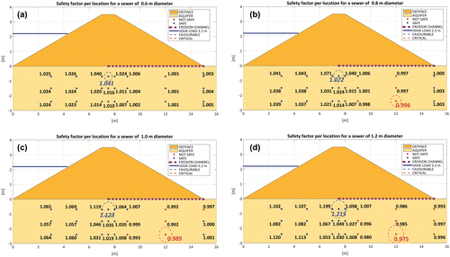
From the obtained results five main observations can be highlighted. The first observation is that for all studied diameters, the highest safety factors were obtained for the shallow locations. In other words, the safest location for all studied diameters will always be located in the most upper location between the aquifer and the bottom of the flood defence.

The second observation is that the increase in diameter is proportional to the increase in safety factor. The highest safety factor (1.215) for all the four different diameters was obtained for the largest pipe diameter (1.2 m). The explanation for this result is the diversion of the incoming flow in two separated portions. One portion of the flow is heading upwards in the direction of the erosion channel whereas the other one is flowing downwards to the bottom of the sewer pipe. After this last portion flows all the way along the perimeter of the sewer pipe, it will try to flow again upwards. In consequence, a higher pressure loss will occur resulting in a lower pressure gradient inside the erosion channel in comparison to the case where no sewer pipe is embedded.

The third observation is that regardless of the diameter of the sewer pipe, the safest condition will always be found when the sewer pipe is located exactly in the midsection of the flood defence, just below the tip of the erosion channel. This can be explained based on the resultant soil filled gap located between the sewer pipe and the impermeable base of the flood defence. This gap determines the amount of flow going directly towards the tip of the erosion channel. This means that the diversion effect is not only a function of the size of the sewer pipe but also of the amount of space left in between the impermeable ‘roof’ and the hard structure. If this space is equal to zero, the embedded structure will work in the same manner as a cut-off wall.

The fourth observation is that there is always a positive effect in terms of safety no matter the size of the sewer pipe, if located anywhere in front of the tip of the erosion channel. The inclusion of a discontinuity before the tip of the erosion channel will always work as an obstacle (energy loss) for the water flowing towards it.

The last observation is that if the sewer pipe is located behind the tip of the erosion channel, it can also have negative effects, especially when located near the bottom of the aquifer (for the IJkdijk case). This corresponds to the critical cases indicated with dashed line pipes with safety factor values lower than 1. This observation is explained by the fact that the IJkdijk flood defence was founded over a shallow aquifer on top of an impermeable basin. In case a large diameter pipe is embedded in the bottom of such a small aquifer, it can also redirect the lower flow upwards in the direction of the erosion channel. Hence, the pressure gradient inside the erosion channel will increase augmenting the erosion capacity. From this it can be concluded that the relative depth of the aquifer with respect to the structure vertical dimension can have an important effect in the flood defence safety as well.

Based on these five observations, it is recommended to locate future sewer pipes (if possible) in the zone in front of the erosion channel tip towards the river side of the flood defence while trying to reduce the ‘gap’ between the bottom of the flood defence and the sewer pipe as much as possible. The size of this gap determines the amount of flow that goes directly towards the erosion channel tip and bottom. If the gap is completely closed, the whole system (flood defence and sewer pipe) will behave similarly to the case where a cut-off wall is present. Analogously, the vertical dimension of the embedded structure is equivalent to the cut-off wall depth. As a final remark, it is important to note that the locations considered unsafe are described by safety factors which are very close to 1 whereas for the safe conditions, the change in safety factor can be as much as 20%. Therefore, there is not sufficient evidence to state that sewer pipes have a negative effect in the piping erosion progression.

5.3. Probabilistic safety assessment

The main goal of probabilistic safety assessment is to determine the likelihood of undesired events which in our case correspond to the progression of the piping erosion failure mechanism. The emulation method, validation, the interpolation and extrapolation capacity of the constructed emulators are presented next which allow to estimate their accuracy and performance for predicting the occurrence of the failure mechanism. The different scenarios are constructed for variations of the aquifer depth, pipe location and permeability uncertainty to understand their combined effect in the failure probability.

5.3.1. FEM emulation method

ANNs used as Ω functions in the present study were trained to predict the pressure gradient inside the erosion channel. The optimal ANN architecture (Chojaczyk et al., 2015) is defined by the combination of number of samples (N) and the number of hidden neurons (HN). Different ANN architectures were tested to find the optimal one that corresponds to the combination which requires less samples and less number of HN while still achieving high performance. By performance it is referred to as the criteria in which the accuracy of the prediction of the model is evaluated. In our case, the selected performance indicator is the coefficient of determination (R²) which indicates the proportion of the variance from the dependent variable(s) that is explained from the independent variables in a function or model. The emulators were trained for 100, 400, 1000, 2500 and 10,000 samples given that their expected standard error from a Monte Carlo simulation is 10, 5, 3.2, 2 and 1%, respectively. The set of N samples were randomly splitted allocating 70% for training and 30% for validating for all architectures. The performance results for the different architectures are presented in Figure 9.

Figure 9. ANN emulator architectures R².

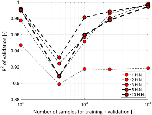
The results show that the 400 samples architecture has the highest difficulty in reproducing the results of the FEM (Figure 9), whereas the 100 samples architecture performs better. This contradiction is expected for the case where highly non-linear processes are being captured as more data represents more information but also more scattering in the data-sets. In that case, an increase in the H.N. is useful as long as the increase does not imply overfitting of the model. Hence, overfitting was checked by comparing the error obtained between training a validation for each architecture (Piotrowski & Napiorkowski, 2013). If the error obtained for the training set is very high (high predictive capacity) and significantly different than the error obtained during validation, it means that the model is overfitted (low generalisation capacity).

For the ANN model of non-embedded structure, the architecture that requires less training input and less hidden neurons is composed by 5 hidden neurons and 1000 samples. This configuration achieves the highest R² (.982). A value of .98 for the R² is high for general model validation, but for the case of emulator training, such a high value is desirable given the fact that it is always possible to afford additional training data.

5.3.2. FEM emulator probabilistic validation

The Sellmeijer 2011 limit state equation (Appendix B) was used for validating the FEM model and emulator limit state functions without embedded sewer pipe. The resulting pdfs (Figure 10) for the three different limit state functions were built based on the 10,000 initially generated input data-set.

Figure 10. (a) PDF of Z for the Sellmeijer revised equation (Thick black line), FEM (Thin blue line) and Emulator (Dashed line). (b) CDF of Z for the Sellmeijer revised equation (Thick black line), FEM (Thin blue line) and Emulator (Dashed line).

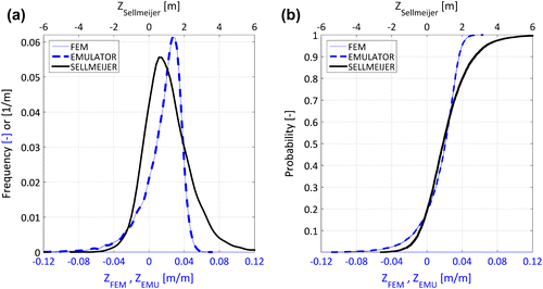
The probability functions for the three models are presented in Figure 10(b) with two different horizontal axis. Note that the Sellmeijer limit state is expressed in different units with respect to the FEM and Emulator distributions. The Emulator and FEM are expressed in terms of pressure gradients inside the erosion channel whereas the Sellmeijer limit state function is expressed terms of total head difference. The distribution generated with the Sellmeijer limit state function presents a Gaussian type of shape whereas the emulator and FEM distributions present a negatively skewed distribution. On one hand, the Sellmeijer limit state equation calculates the residual strength in terms of the total head. On the other hand, the FEM and the emulator calculate the limit state as the residual resistance in terms of pressure gradients (m/m) inside the erosion channel. However, they are still comparable as the general form of the limit state equations allows to define the failure threshold (Z ≤ 0) no matter the limit state function. In other words, the failure probability is defined for all models by the exact same point where the resistance is equal to or less than the load. In Figure 10(b), it can be observed how the three functions intersect in two common points including the failure threshold (Z ≤ 0). The corresponding probabilities of failure value from FEM, emulator and Sellmeijer are equal to .189, .186 and .193, respectively. Consequently, it is concluded that the emulator can be used for failure probability estimation as for the case of non-structural embedment is producing very close values of failure probability when compared to the revised Sellmeijer limit state equation.

5.3.3. FEM emulator interpolation and extrapolation capacity

The emulators were trained for distributions modified by the (λ) as explained in Section 4.2. However, the interpolation and extrapolation capacity from the emulator was tested. The tests consisted in calculating the probability of failure for different CV for the three main parameters assumed as stochastic. For each parameter test, one single variable was sampled for different CV values while fixing the other two as constant with mean value presented in Table 2. The results are presented in Figure 11.

Figure 11. Failure probabilities as a function of the main random variables with different CV.

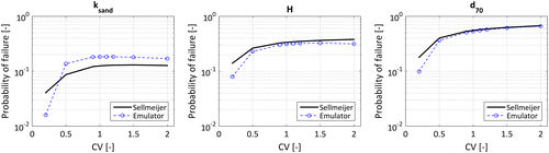
In terms of extrapolation the emulator performs very well for large CV. For less spreaded distributions of the parameters, the emulator results in larger difference in the estimated failure probabilities with respect to Sellmeijer function. In particular for the case of the sand permeability where the Sellmeijer limit state gives a failure probability of .0406 whereas the emulator results in .16. After comparing the change in failure probability for three main parameters, it can be concluded that the sand permeability is the one that accounts for the largest variability (change by order of magnitude for smallest and largest CV) in the estimated failure probability for both Sellmeijer and the emulator. Hence, the emulator will only be implemented for CVs between .5 and 1.5.

5.3.4. FEM emulation with structural embedment

In the previous section, it was shown that the two forces equilibrium concept and the Darcy flow with fictitious permeability model are consistent with the Sellmeijer limit state equation (Appendix B) when representing the no-embedment case. It is assumed that the inclusion of an embedded structure is equivalent to a change in the aquifer permeability and flow pattern behaviour but the failure concept still holds. Hence, the same emulation methodology was used for the cases where structural embedment is present.

Twelve different ANN emulators were trained based on 10,000 samples propagated through their original FEM models. Each FEM model corresponds to one of the three selected aquifer depths (D). For 9 of the 12 cases, a sewer pipe of 1.2 m is used in different locations. The three remaining ones correspond to the case where no structure is embedded. A cover of 30 cm below the flood defence at a burial depth of 1.5 m to the bottom of the pipe was chosen. All models were trained with 70% of the training data and validated with the remaining 30% with a fixed N set of 1000 samples. Therefore, the results presented in Table 3 correspond to the average R² value obtained after training each emulator a 100 times. Note that the size of the erosion channel (n_g) is varied as a function of the aquifer depths based on the results presented in Section 5.1.3.

Table 3. Validation results of emulators (Ω) versus FEM output as a function of different number of hidden layers (H.L.).

						R^2 validation value for vs.
Sewer pipe	X (m)	Y (m)	GAP (m)	D (m)	ng (–)	1 H.L.	2 H.L.	3 H.L.	4 H.L.	5 H.L.
NO	–	–	.3	3	8.2	.914	.986	.992	.996	.998
YES	0	−.9	.3	3	8.2	.915	.986	.994	.997	.996
YES	7.5	−.9	.3	3	8.2	.916	.978	.993	.996	.998
YES	15	−.9	.3	3	8.2	.915	.978	.994	.996	.998
NO	–	–	.3	5	9.4	.918	.982	.993	.990	.997
YES	0	−.9	.3	5	9.4	.919	.985	.992	.996	.997
YES	7.5	−.9	.3	5	9.4	.921	.980	.995	.996	.997
YES	15	−.9	.3	5	9.4	.919	.982	.995	.997	.997
NO	–	–	.3	8	10	.920	.986	.993	.996	.996
YES	0	−.9	.3	8	10	.919	.974	.991	.996	.996
YES	7.5	−.9	.3	8	10	.922	.976	.993	.997	.997
YES	15	−.9	.3	8	10	.920	.976	.995	.997	.997

Table 3 shows that in average, three hidden nodes represent the most optimal architecture in general while satisfying R²≥ .98. We found that it is possible to obtain high predictive capacity with only 1000 training samples for both embedded and non-embedded cases reducing the computational burden significantly.

5.3.5. Reliability index (β) for structural embedment

The safety of each flood defence was quantified based on the Hasofer-Lind reliability index (β) (Tichý, 1988) instead of the failure probability. A higher β index represents a safer structure. This index is equivalent to the reduced standardised variable that corresponds to the structure failure probability in the standardised normal distribution. To quantify the combined effect of the embedded sewer pipe and the permeability uncertainty, the defence safety was assessed for different CVs for the 12 trained emulators (Table 3) as presented in Figure 12.

Figure 12. β indexes for different aquifer depths and permeability CVs.

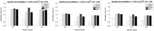
These results show how locating the sewer pipe in the midsection will always be safer than in the other two locations, despite the heterogeneity (CV of permeability) of the soil. Furthermore, the marginal effect (difference between no sewer pipe and with sewer pipe) increases with the increment in aquifer depth. For aquifers equal of deeper than 8 m, the increment in β index with respect to the case of no embedded sewer pipe will be very similar despite the location of the sewer pipe. These results show that the aquifer depth has a significant influence on the safety of the structure and consequently the assumption of representing it as a deterministic value might change the assessment. Yet, the effect is only relevant until a certain depth and therefore the random distribution should be bounded based on the results presented in Section 5.1.3.

All three assessments for locations with sewer pipes show that the inclusion of the hard structure inside the foundation will always improve the safety with respect to the case of non-structural embedment no matter the degree of heterogeneity of the soil permeability. This result differs with the conclusion obtained from the deterministic location in Section 5.2, where it was observed that most structures located in the hinterside resulted in unsafer situations. This difference can be explained due to the fact that once the permeability factor becomes a random variable, the changes in the inner pressures of the aquifer are not equally affected by the embed sewer pipe. This cannot be observed under deterministic conditions. Additionally, the uncertainty in the aquifer permeability is the one that has the highest impact in the variability of the resultant failure probability.

In case of a less heterogeneous soil represented by a CV of .5, the maximum difference in β indexes is obtained for an aquifer of 5 m. In this case, the non-sewer embedment results in a β index of .978 whereas the one with the sewer pipe located in the middle results in a β index of 1.28. If compared to the cases where the pipe is located in front and in the back of the tip of the erosion channel, the effect is less significant but still positive as both produce a β index of 1.16. Note that the results of this analysis reflect low beta indexes or in other words in very ‘Unsafe’ situations.

In a more robust piping erosion assessment, the total failure probability is conditional to the failure mechanisms of heave and/or uplift (Schweckendiek et al., 2014). As a consequence, the resultant safety β index will be higher (safer structure) as the probability of the total failure mechanism is conditional on the occurrence of the other two failure mechanisms. In the Netherlands, flood defences are designed for β indexes of 3 and above depending on the associated flood risk (López De La Cruz, Calle, & Schweckendiek, 2011). In those cases, the failure probabilities will be located more towards the left tail of the Z reliability PDF and consequently higher beta indexes are expected. If so, it is expected that the difference in safety between the case of embedment and non-embedment will be more significant than the ones encountered in this study.

6. Conclusions

A limit state piping erosion FEM modelling methodology has been developed and validated against the obtained results from the same conditions evaluated in the Sellmeijer 2011 limit state equation (Appendix B). This methodology allows to include the effect on safety originated from sewer pipes under flood defences. The methodology was implemented for both deterministic and probabilistic safety assessments which allowed to answer the three main research questions. The main and general conclusion of the present study is that the presence of sewer pipes under flood defences has a significant effect on the safety of the flood defence in terms of piping erosion. This conclusion holds for both deterministic and probabilistic safety assessments. The results also indicate that it can even have beneficiary effects in terms of safety depending on the location and relative size with respect to the aquifer depth. For the three research questions it can be stated that:

(1)	The fictitious permeability approach for FEM modelling proves to be a reliable method for assessing piping erosion in steady state conditions. A value of 8.2 times of the d70 particle size diameter for the average erosion channel height was obtained based on the experimental conditions for the IJkdijk experiment. This value agrees with other experimental findings and it is recommended as an initial guess for implementing the fictitious permeability approach for limit state piping erosion modelling. We also showed that assuming an average cross section which is significantly wider in respect to its height gives poor results for 2D modelling of piping erosion. This last conclusion is in agreement with the results presented in other earlier studies about piping erosion cross section (Van Beek et al., 2014).
(2)	The sewer pipe size and location play an important role in the safety of the flood defence for piping erosion. Both will change the flow patterns and magnitudes inside the aquifer and consequently the exerted pressure gradient inside the erosion channel will be affected as well. In particular if located after the middle of the flood defence towards the river side. The results for the deterministic assessment show that the most important geometrical aspect for the flood defence safety is the originated gap between the embedded structure and the flood defence base. This gap will determine the portion of flow which will go directly towards the erosion channel. The remaining portion will be forced to go downwards under the structure. In that sense, the size of the structure defines the additional energy loss in the aquifer. In a complementary way, it can also be concluded that for the case of deeply embedded structures, no matter their size or location there is almost no effect in the piping erosion inner pressure as the gap becomes too big and there will be no flow diversion.
(3)	In terms of the probabilistic assessments, it is also shown that the uncertainties associated to the sand permeability and water load have a significant effect in the safety (β index) of the flood defence with the sewer pipe located underneath. The consideration of the soil heterogeneity and water probabilistic distribution influences the increase or reduction of the inner pressure gradient of the erosion channel. This change is relative to the one originated by the embedded structure size and location. Emulation of FEM models proved to be a feasible approach for assessing this kind of complex structures. It was also proven that the method produces the same probabilistic result for non-structural embedment when compared to the revised Sellmeijer limit state equation (Appendix A). For realistic values such as the ones measured for the IJkdijk experiment, the structural embedment proved to have significant effects for the commercial sewer pipe diameters used in this study.

Disclosure statement

No potential conflict of interest was reported by the authors.

Funding

This research is supported by the Dutch Technology Foundation STW, which is part of the Netherlands Organisation for Scientific Research (NWO), and which is partly funded by the Ministry of Economic Affairs.

Acknowledgements

The authors would like to thank STW foundation, Raymond Van der Meij from the Dike Safety department of Deltares, the Integral and sustainable design of Multi-functional flood defences programme and the anonymous reviewers whose comments greatly improved the quality and clarity of the present manuscript.

Appendix A. Friction loss coefficients (β_fi) for different cross sections

Table A1. Different cross section parameters used for fictitious permeability calculation with their corresponding β_fi (Bersan et al., 2013; Muzychka & Yovanovich, 2009).

Table

Channel Cross section	b/a	Dh	βfi
Square	1	a	56.92
Rectangular	16		85.58
Circular	1	a	64.00
Ellipsoid	16		76.77
Fracture	∞	2a	96.00

Appendix B. Sellmeijer limit state function 2011

In 2011, the original equation was modified and calibrated (Sellmeijer et al., 2011) based on the two forces approach explained previously in Section 3.2. The updated expressions are presented in Equations (B1(B1) )–(B5(B5) ) as:(B1) (B2) (B3) (B4) (B5)

Table B1. Sellmeijer 2011 revised equation nomenclature.

Table

Zp	(–)	Residual resistance (Limit State)
ƞ	(kN/m^3)	White’s sand packing coefficient (.25)
γ’s	(kN/m^3)	Unitary weight of submerged sand particles
γw	(deg)	Unitary weight of water
θ	(m)	Bedding angle of sand grains
d70	(m)	70 per cent quintile value grain size distribution of sand layer
d70 m	(m^2/s)	Calibration reference value (2.08 × 10^−4 m)
ν	(m/s)	Kinematic viscosity of water at 20 °C
K	(m/s^2)	Hydraulic conductivity of sand
g	(m)	Gravitational acceleration (9.81 m/s^2)
D	(–)	Average thickness of sand aquifer
mp	(m)	Modelling uncertainty factor
Hc	(–)	Critical hydraulic head difference
FR	(–)	Resistance factor
FS	(–)	Scale factor
FG	(m)	Geometric factor
Hc	(m)	Critical PE resistance head
L	(m)	Seepage length from entrance point to sand boil water exit
H	(m)	Water level in the riverside of the flood defence
hb	(m)	Water level at hinterside outflow point
bimp	(m)	Impermeable layer thickness at the sand boil exit point

Note: the product of the hydraulic conductivity of soil and kinematic viscosity from the same fluid at the same temperature divided by the gravitational acceleration is equivalent to the intrinsic permeability k (m²) (noted as lower case k).

References

- Aguilar-López, J. P., Warmink, J. J., Schielen, R. M. J., & Hulscher, S. J. M. H. (2016). Soil stochastic parameter correlation impact in the piping erosion failure estimation of riverine flood defences. Structural Safety, 60, 117–129. doi:10.1016/j.strusafe.2016.01.004
- Bear, J., & Verruijt, A. (1987). Modeling groundwater flow and pollution (Vol. 2). Dordrecht: Springer Science & Business Media.10.1007/978-94-009-3379-8
- Bersan, S., Jommi, C., Koelewijn, A., & Simonini, P. (2013). Applicability of the fracture flow interface to the analysis of piping in granular material. COMSOL Conference 2013, Rotterdam.
- Bligh, W. (1910). Dams, barrages and weirs on porous foundations. Engineering News, 64, 708–710.
- Bucher, C., & Most, T. (2008). A comparison of approximate response functions in structural reliability analysis. Probabilistic Engineering Mechanics, 23, 154–163. doi:10.1016/j.probengmech.2007.12.022
- Chen, N., Gunzburger, M., Hu, B., Wang, X., & Woodruff, C. (2012). Calibrating the exchange coefficient in the modified coupled continuum pipe-flow model for flows in karst aquifers. Journal of Hydrology, 414–415, 294–301. doi:10.1016/j.jhydrol.2011.11.001
- Cho, S. E. (2009). Probabilistic stability analyses of slopes using the ANN-based response surface. Computers and Geotechnics, 36, 787–797. doi:10.1016/j.compgeo.2009.01.003
- Chojaczyk, A. A., Teixeira, A. P., Neves, L. C., Cardoso, J. B., & Guedes Soares, C. (2015). Review and application of artificial neural networks models in reliability analysis of steel structures. Structural Safety, 52, Part A, 78–89. doi:10.1016/j.strusafe.2014.09.00210.1016/j.strusafe.2014.09.002
- El Shamy, U., & Aydin, F. (2008). Multiscale modeling of flood-induced piping in river levees. Journal of Geotechnical and Geoenvironmental Engineering, 134, 1385–1398.10.1061/(ASCE)1090-0241(2008)134:9(1385)
- Elishakoff, I. (2012). Safety factors and reliability: Friends or foes? Dordrecht: Springer Science & Business Media.
- Forrester, A., Sobester, A., & Keane, A. (2008). Engineering design via surrogate modelling: A practical guide. West Sussex: Wiley.10.1002/9780470770801
- Hoffmans, G. J. C. M. (2014). An overview of piping models. 7th International Conference on Scour and Erosion, Perth, Australia.
- Jianhua, Y. (1998). FE modelling of seepage in embankment soils with piping zone. Chinese Journal of rock mechanics and engineering, 17, 679–689.
- Kaunda, R. B. (2015). A neural network assessment tool for estimating the potential for backward erosion in internal erosion studies. Computers and Geotechnics, 69, 1–6. doi:10.1016/j.compgeo.2015.04.010
- Kingston, G. B., Rajabalinejad, M., Gouldby, Ben P.;Van Gelder, P. H. (2011). Computational intelligence methods for the efficient reliability analysis of complex flood defence structures. Structural Safety, 33, 64–73. doi:10.1016/j.strusafe.2010.08.002
- Koelewijn, A., De Vries, G., Van Lottum, H., Förster, U., Van Beek, V. M., & Bezuijen, A. (2014). Full-scale testing of piping prevention measures: Three tests at the IJkdijk. Proceedings of the Physical Modeling in Geotechnics, 2, 891–897.10.1201/b16200
- Lachouette, D., Golay, F., & Bonelli, S. (2008). One-dimensional modeling of piping flow erosion. Comptes Rendus Mécanique, 336, 731–736. doi:10.1016/j.crme.2008.06.007
- Lane, E. W. (1935). Security from under-seepage-masonry dams on earth foundations. Transactions of the American Society of Civil Engineers, 100, 1235–1272.
- Li, D., Chen, Y., Lu, W., & Zhou, C. (2011). Stochastic response surface method for reliability analysis of rock slopes involving correlated non-normal variables. Computers and Geotechnics, 38, 58–68. doi:10.1016/j.compgeo.2010.10.006
- Liedl, R., Sauter, M., Hückinghaus, D., Clemens, T., & Teutsch, G. (2003). Simulation of the development of karst aquifers using a coupled continuum pipe flow model. Water Resources Research, 39(3), n/a–n/a. doi:10.1029/2001WR001206
- Lominé, F., Scholtès, L., Sibille, L., & Poullain, P. (2013). Modeling of fluid–solid interaction in granular media with coupled lattice Boltzmann/discrete element methods: Application to piping erosion. International Journal for Numerical and Analytical Methods in Geomechanics, 37, 577–596.10.1002/nag.v37.6
- López De La Cruz, J., Calle, E., & Schweckendiek, T. (2011, June 2–3). Calibration of piping assessment models in the Netherlands. Proceedings of the 3rd International Symposium on Geotechnical Safety and Risk, ISGSR 2011. Bundesanstalt für Wasserbau, Munich, Germany.
- Low, B. K. (2014). FORM, SORM, and spatial modeling in geotechnical engineering. Structural Safety, 49, 56–64. doi:10.1016/j.strusafe.2013.08.008
- Lü, Q., & Low, B. K. (2011). Probabilistic analysis of underground rock excavations using response surface method and SORM. Computers and Geotechnics, 38, 1008–1021. doi:10.1016/j.compgeo.2011.07.003
- Mott, R. L., Noor, F. M., & Aziz, A. A. (2006). Applied fluid mechanics. Singapore: Pearson Prentice Hall.
- Muzychka, Y., & Yovanovich, M. (2009). Pressure drop in laminar developing flow in noncircular ducts: A scaling and modeling approach. Journal of Fluids Engineering, 131, 111105-1–111105-11.10.1115/1.4000377
- Ojha, C. S. P., Singh, V. P., & Adrian, D. D. (2008). Assessment of the role of slit as a safety valve in failure of levees. International Journal of Sediment Research, 23, 361–375. doi:10.1016/S1001-6279(09)60007-X
- Piotrowski, A. P., & Napiorkowski, J. J. (2013). A comparison of methods to avoid overfitting in neural networks training in the case of catchment runoff modelling. Journal of Hydrology, 476, 97–111. doi:10.1016/j.jhydrol.2012.10.019
- Samardzioska, T., & Popov, V. (2005). Numerical comparison of the equivalent continuum, non-homogeneous and dual porosity models for flow and transport in fractured porous media. Advances in Water Resources, 28, 235–255. doi:10.1016/j.advwatres.2004.11.002
- Schoefs, F., Le, K. T., & Lanata, F. (2013). Surface response meta-models for the assessment of embankment frictional angle stochastic properties from monitoring data: An application to harbour structures. Computers and Geotechnics, 53, 122–132. doi:10.1016/j.compgeo.2013.05.005
- Schweckendiek, T., Vrouwenvelder, A. C. W. M., & Calle, E. O. F. (2014). Updating piping reliability with field performance observations. Structural Safety, 47, 13–23. doi:10.1016/j.strusafe.2013.10.002
- Sellmeijer, J., López de la Cruz, J. L., van Beek, V. M., & Knoeff, H. (2011). Fine-tuning of the backward erosion piping model through small-scale, medium-scale and IJkdijk experiments. European Journal of Environmental and Civil Engineering, 15, 1139–1154. doi:10.1080/19648189.2011.9714845
- Sellmeijer, J. (1988). On the mechanism of piping under impervious structures. TU Delft, Delft University of Technology, Delft..
- Sellmeijer, J. (2006). Numerical computation of seepage erosion below dams (piping). In G. H. Gouda (Ed.), Third International Conference on Scour and Erosion 2006 (pp. 596–601). Amsterdam, The Netherlands: CUR Bouwn & Infra.
- Sellmeijer, J., & Koenders, M. A. (1991). A mathematical model for piping. Applied Mathematical Modelling, 15, 646–651. doi:10.1016/S0307-904X(09)81011-1
- Shamekhi, E., & Tannant, D. D. (2015). Probabilistic assessment of rock slope stability using response surfaces determined from finite element models of geometric realizations. Computers and Geotechnics, 69, 70–81. doi:10.1016/j.compgeo.2015.04.014
- Terzaghi, K., Peck, R. B., & Mesri, G. (1996). Soil mechanics in engineering practice. New York: Wiley.
- Tichý, M. (1988). On the reliability measure. Structural Safety, 5, 227–232. doi:10.1016/0167-4730(88)90011-2
- Van Beek, V. M. (2015). Backward erosion piping: Initiation and progression (PhD dissertation). TU Delft, Delft University of Technology, Delft.
- Van Beek, V. M., Vandenboer, K., & Bezuijen, A. (2014, December 2–4). Influence of sand type on pipe development in small-and medium-scale experiments. Scour and Erosion: Proceedings of the 7th International Conference on Scour and Erosion (pp. 111). Perth, Australia: CRC Press.10.1201/b17703
- Van Beek, V. M., Knoeff, H., & Sellmeijer, H. (2011). Observations on the process of backward erosion piping in small-, medium- and full-scale experiments. European Journal of Environmental and Civil Engineering, 15, 1115–1137. doi:10.1080/19648189.2011.9714844
- Van Esch, J., Sellmeijer, J., & Stolle, D. (2013). Modeling transient groundwater flow and piping under dikes and dams. 3rd International Symposium on Computational Geomechanics (ComGeo III). Krakow: International Centre for Computational Engineering.
- Van Loon-Steensma, J. M., & Vellinga, P. (2014). Robust, multifunctional flood defenses in the Dutch rural riverine area. Natural Hazards and Earth System Science, 14, 1085–1098. doi:10.5194/nhess-14-1085-2014
- Van Veelen, P., Voorendt, M., & Van der Zwet, C. (2015). Design challenges of multifunctional flood defences. A comparative approach to assess spatial and structural integration. Research in Urbanism Series, 3, 275–292
- Vandenboer, K., Van Beek, V. M., & Bezuijen, A. (2014). 3D finite element method (FEM) simulation of groundwater flow during backward erosion piping. Frontiers of Structural and Civil Engineering, 8, 160–166. doi:10.1007/s11709-014-0257-7
- Wang, D.-Y., Fu, X.-D., Jie, Y.-X., Dong, W.-J., & Hu, D. (2014). Simulation of pipe progression in a levee foundation with coupled seepage and pipe flow domains. Soils and Foundations, 54, 974–984.10.1016/j.sandf.2014.09.003
- White, C. M. (1940). The equilibrium of grains on the bed of a stream. Proceedings of the Royal Society of London. Series A, Mathematical and Physical Sciences, 174, 322–338. doi:10.2307/97393
- Yazdi, J., & Salehi Neyshabouri, S. A. A. (2014). Adaptive surrogate modeling for optimization of flood control detention dams. Environmental Modelling & Software, 61, 106–120. doi:10.1016/j.envsoft.2014.07.007
- Zhang, J., Chen, H. Z., Huang, H. W., & Luo, Z. (2015). Efficient response surface method for practical geotechnical reliability analysis. Computers and Geotechnics, 69, 496–505. doi:10.1016/j.compgeo.2015.06.010
- Zhou, X.-J., Jie, Y.-X., & Li, G.-X. (2012). Numerical simulation of the developing course of piping. Computers and Geotechnics, 44, 104–108. doi:10.1016/j.compgeo.2012.03.010