Influence of drag closures and inlet conditions on bubble dynamics and flow behavior inside a bubble column

ABSTRACT

In this paper, the hydrodynamics of a bubble column is investigated numerically using the discrete bubble model, which tracks the dispersed bubbles individually in a liquid column. The discrete bubble model is combined with the volume of fluid approach to account for a proper free surface boundary condition at the liquid–gas interface. This improves describing the backflow region, which takes place close to the wall region. The numerical simulation is conducted by means of the open source computational fluid dynamics library OpenFOAM®. In order to validate the numerical model, experimental results of a bubble column are used. The numerical prediction shows an overall good agreement compared to the experimental data. The effect of injection conditions and the influence of the drag closures on bubble dynamics are investigated in the current paper. Here, the significant effect of injection boundary conditions on bubble dynamics and flow velocity in the studied cavity is revealed. Moreover, the impact of the choice of the drag closure on the liquid velocity field and on bubble behavior is indicated by comparing three drag closures derived from former studies.

KEYWORDS:

• Bubble column
• drag closures
• discrete bubble model
• OpenFOAM®
• Volume of Fluid

1. Introduction

Bubbly multiphase flows are frequently encountered in many applications. For instance, they can be found in multiphase reactors with the aim of enhancing the mixing of different elements in the chemical industry or in metallurgy. Despite simple geometry of these configurations, the bubbles within the reactors exhibit a complex dynamic which is determined by the momentum exchange between the bubbles and liquid (Shah, Kelkar, Godbole, & Deckwer, 1982).

Computational fluid dynamics (CFD) models play a significant role in order to understand the dynamics of the bubble columns in these processes in detail. One approach is the macro-scale two-fluids model (Euler–Euler), which treats both phases as continua (Pan, Dudukovic, & Chang, 1999; Renze, Buffo, & Marchisio, 2014; Sokolichin & Eigenberge, 1999). This approach is typically employed to simulate industrial scale flow. Another approach is the meso-scale discrete bubble model (DBM) (Delnoij, Kuipers, & Swaaij, 1999; Delnoij, Lammers, Kuipers, & Swaaij, 1997). Here, the phases are treated separately. In this model, the bubbles are tracked as individual point particles by their equation of motion including drag, lift, buoyancy and other forces acting on the moving bubble. Unresolved effects such as bluff bodies that flow past the bubble are captured by suitable empirical parameters. The interaction between the phases is considered through a term that appears in the momentum equation. Furthermore, transient bubble deformation is not taken into account. In the DBM model, bubble break-up and coalescence can be treated individually. The DBM model can be considered as a transition between the macro-scale Euler–Euler model and the fully resolved DNS simulation. In the DNS simulation, the fully resolved deformation of bubble shape can be taken into account, for instance, by means of the immersed boundary method (Schwarz & Fröhlich, 2013). The disadvantage of a DNS simulation is the high computational effort, especially in the case of a larger computational domain. For more details about modeling of multi-phase flows, the reader is referred to Yeoh and Jiyuan (2009), and Tryggvason, Scardovelli, and Zaleski (2011).

Extensive experimental studies have been carried out in order to derive drag closures for moving bubbles in a liquid, which can be used in numerical investigations (Ishii & Zuber, 1979; Simonnet, Gentric, Olmos, & Midoux, 2007; Tomiyama, Kataoka, Zun, & Sakaguchi, 1998). Tomiyama et al. (1998) conducted a single bubble experiment to derive a drag coefficient in terms of the Eötvös number Eo = gΔρd_b²/σ_f and the Reynolds number Re_b = |u_f-u_b|d_b/υ_f. The developed closure is derived for the ranges of 10⁻² < Eo < 10³ and 10⁻³ < Re_b < 10⁵. Other experiments have investigated bubble swarms ascending through a cavity filled with water (Ishii & Zuber, 1979; Simonnet et al., 2007). Ishii and Zuber (1979) developed correlations to estimate the drag coefficient of a bubble ascending in a bubble swarm. The application range of this model is not mentioned explicitly. However, it is expected to be valid approximately for Re_b < 10⁴ and Eo < 10⁶. Here, the derived correlations take into account the bubble shape (spherical, ellipsoidal or cap). The effect of bubble diameter, relative velocity and local void fraction on the bubble dynamics is shown in a paper conducted by Simonnet et al. (2007). In this paper, the derived correlation is assumed to work well for Re_b < 8 x10⁴ and Eo < 10⁶.

Other drag closures have been obtained by means of numerical investigation (Dijkhuizen, Roghair, van Sint Annaland, & Kuipers, 2010; Roghair et al., 2011; Sankaranarayanan, Shan, Kevrekidis, & Sundaresan, 1999; Sankaranarayanan, Shan, Kevrekidis, & Sundaresan, 2002). Dijkhuizen et al. (2010) used an improved front tracking model in order to study the drag force acting on an isolated single bubble ascending in an initially quiescent liquid. They proposed to combine Re_b and Eo dependent parts of the drag closure to cover the transition from spherical to deformed bubbles. Using the improved front tracking model with direct numerical simulation (DNS), Roghair et al. (2011) developed a correction function depending on Eo and the local void fraction α_loc to account for bubble swarm effects. The derived function is valid for 1 < Eo < 4 and 150 < Re_b < 1200. Other drag closures of bubble rising in a stagnant liquid as well as a better description of bubble dynamics can be found in Clift, Grace, and Weber (2005).

Many attempts have been made to study bubble swarms ascending in a stagnant liquid, either using the DBM model (Besbes, Hajem, Ben Aissia, Champagne, & Jay, 2015; Jain, Kuipers, & Deen, 2014; Lau, Bai, Deen, & Kuipers, 2014; Lau, Roghair, Deen, van Sint Annaland, & Kuipers, 2011; Sommerfield, Bourloutski, & Bröder, 2003) or the Euler–Euler approach (Deen, Solberg, & Hjertager, 2001; Ma, Lucas, Ziegenhein, Fröhlich, & Deen, 2015; Masood & Delgado, 2014; Zhang, Deen, & Kuipers, 2006; Ziegenhein, Rzehak, & Lucas, 2015; Ziegenhein, Rzehak, Krepper, & Lucas, 2013). Masood and Delgado (2014) used the Euler–Euler approach to describe the dynamics of bubbles rising in a cavity. The authors compared three drag closures derived in previous works conducted by Ishii and Zuber (1979), Schiller and Naumann (1935), Grace, Wairegi, and Nguyen (1976). It was found that the drag closure derived in Ishii and Zuber (1979) was able to predict the flow velocity better than the other considered drag closures. A paper conducted by Pourtousi, Sahu, and Ganesan (2014) reviewed previous works using the Euler–Euler approach to show the significant effect of interfacial forces and turbulence models on gas–liquid velocity in a bubble column. Here, it is mentioned that using drag closure as the only interfacial model is not enough to describe the bubble plume oscillations as observed in the experiment.

The DBM model was used in the literature to investigate many applications. For instance, this model was employed in steelmaking to study bubbly flow in the metallurgical processes (Chatterjee & Chattopadhyay, 2015; Chatterjee & Chattopadhyay, 2016; Chattopadhyay & Guthrie, 2011). Additionally, the DBM model was used to investigate some applications in the field of chemical and process engineering (Greifzu, Kratzsch, Forgber, Lindner, & Schwarze, 2016; Shalaby, Wozniak, & Günter, 2008; Movahedirad, Ghafari, & Dehkordi, 2012; Van der Hoef, van Sint Annaland, Deen, & Kuipers, 2008).

Most of the previous numerical investigations were achieved either by means of commercial CFD packages or by means of in-house developed codes. Moreover, drag closures used in most of the previous works did not consider the bubble swarm effect, which influences bubble dynamics considerably. In addition, the previous papers did not account for the effect of the inlet boundary conditions on the bubble dynamics and on the flow behavior in a bubble column.

Therefore, the main goal of the present paper is to introduce a DBM model implemented in the open source computational fluid dynamics library OpenFOAM® to describe the hydrodynamics of a bubble column. The Volume of Fluid approach (VOF) is combined with the DBM model to account for a proper free surface boundary condition at the liquid–gas interface. This can enhance describing the recirculation region, which takes place close to the walls in the bubble column. The present paper shows the considerable effect of the inlet boundary condition on bubble dynamics and flow behavior in the bubble column. In order to consider the bubble swarm effects, a recent drag correlation proposed by Roghair et al. (2011) is included in the numerical model to consider bubble swarm effects. Furthermore, the latter drag closure is compared with other common drag closures. The numerical results are validated by means of the particle image velocimetry (PIV) measurement conducted by Deen et al. (2001).

2. Governing equation

2.1. Fluid phase

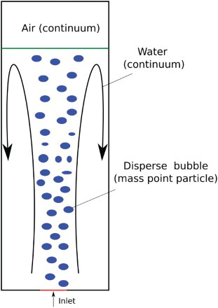
In the DBM model, the continuous phase of the bubble column is described in a Eulerian framework. The fluid phase is denoted by subscript [f] in the following equations. The fluid phase can be either the continuous gas (g) above the liquid column or liquid phase (l) in the column, which are separated by a resolved phase interface. A schematic sketch is presented in Figure 1 to illustrate the numerical model considered here. In the present study, the delayed detached eddy simulation (DDES) model is used to describe the turbulent fluid motion (Spalart et al., 2006). The main principle of this model is that the Spalart–Allmaras turbulence model is adopted in the wall vicinity, while large-eddy simulation (LES) is applied in the bulk of the flow. Therefore, filtered LES momentum and mass conservation equations are adopted in the core region, whereas unsteady Reynolds-Averaged Navier-Stokes (URANS) equations are employed in the boundary layer. Theses equations are expressed as: (1) $\mathrm{\nabla }\cdot {\underset{\_}{u}}_f=0$(1) (2) $\frac{\mathrm{\partial }{\underset{\_}{u}}_f}{\mathrm{\partial }t}+({\underset{\_}{u}}_f\cdot \mathrm{\nabla }){\underset{\_}{u}}_f=-\frac{1}{{\rho }_f}\mathrm{\nabla }p+\mathrm{\nabla }\cdot ({\nu }_f\mathrm{\nabla }{\underset{\_}{u}}_f+{\underset{\_}{\underset{\_}{\tau }}}^{\mathrm{model}})+{\underset{\_}{F}}_{\sigma }+\underset{\_}{M}.$(2) Here, u_f and p are the Reynolds-averaged (URANS) or filtered (LES) velocity and pressure of the fluid, respectively. υ_f is the kinematic viscosity and ρ_f is the density of the liquid. F_σ is the surface tension force following from the VOF approach, which is adopted to capture the free surface behavior. M accounts for the coupling term, which is responsible for momentum transfer between the continuous and disperse phase. τ^model denotes the subgrid stress tensor for the LES mode or the Reynolds stress tensor for the URANS mode.

Figure 1. Schematic sketch of the numerical model to show the phases considered in the present work.

2.2. Bubble phase

In the DBM model, each bubble is tracked as a mass point in a Lagrangian way. Here, the surface of the bubbles and their deformation are not explicitly simulated. The bubble motion is calculated from a force balance for a bubble: (3) $m_b\frac{\mathrm{d}{\underset{\_}{u}}_b}{\mathrm{d}t}={\underset{\_}{F}}_{\mathrm{tot}}={\underset{\_}{F}}_G+{\underset{\_}{F}}_B+{\underset{\_}{F}}_D+{\underset{\_}{F}}_{VM}+{\underset{\_}{F}}_L+{\underset{\_}{F}}_p.$(3) Here, F_G and F_B are the gravitational and the buoyancy forces, respectively. F_VM is the virtual mass force, which is caused by the accelerated motion of the bubble. F_L denotes the lift force. F_p represents the pressure gradient force. F_D is the drag force exerted by the liquid on the bubble. After estimating the force acting on each bubble i present in a cell of the computational grid, the coupling term is computed as follows: (4) $\underset{\_}{M}=-\frac{1}{V_{\mathrm{cell}}}\sum _{\mathrm{\forall }i}{\underset{\_}{F}}_{{\mathrm{tot}}_i},$(4) where V_cell is the volume of the computational cell.

2.2.1. Buoyancy force and gravitational force

The buoyancy force F_B and the gravitational force F_G are calculated in OpenFOAM® using the following equation: (5) ${\underset{\_}{F}}_B+{{\underset{\_}{F}}_G}_{=}\frac{({\rho }_b-{\rho }_f)\pi d_b^3}{6}\underset{\_}{g}.$(5)

2.2.2. Drag force

The drag force arises from the form drag and friction drag due to pressure distribution around the bubble and shear stress. It is calculated by: (6) ${\underset{\_}{F}}_D=-\frac{1}{8}{C}_D{\rho }_f\pi d_b\left|{\underset{\_}{u}}_b-{\underset{\_}{u}}_f\right|({\underset{\_}{u}}_b-{\underset{\_}{u}}_f).$(6) In the present study, the drag coefficient C_D is calculated by using three closures. The first drag closure is derived experimentally from Tomiyama et al. (1998) (drag model 1) in terms of Eo and Re_b and is addressed as follows: (7) $\begin{array}{rl}{C}_D^1& =max\left\{min\left[\frac{24}{R{e}_b}\left(1+0.15R{e}_b^{0.687}\right),\frac{48}{R{e}_b}\right],\right.\\ & \left.\frac{8}{3}\frac{Eo}{Eo+4}\right\}.\end{array}$(7) The second drag closure is developed by Ishii and Zuber (1979) (drag model 2) and depends on the bubble shape. It is formulated as follows: (8) $C_D^2=max\left\{\frac{24}{{Re}_b}(1+0.15R{e}_b^{0.687}),min\left[\frac{4}{3}\sqrt{2Eo},\frac{8}{3}\right]\right\}.$(8) The third drag closure is developed by Roghair et al. (2011) (drag model 3) in order to account for the effect of bubble swarms. This is achieved by including a correction function depending on Eo and the local void fraction α_loc: (9) $\frac{C_D^3}{C_{D,\mathrm{\infty }}(1-{\alpha }_{loc})}=f(Eo,{\alpha }_{loc})=1+\left(\frac{18}{Eo}\right){\alpha }_{loc}.$(9) α_loc is estimated instantaneously during the simulation for each computational cell.

C_D,∞ is the drag closure of single bubble calculated as follows: (10) $C_{D,\mathrm{\infty }}=\sqrt{C_D{\left(R{e}_b\right)}^2+C_D{\left(Eo\right)}^2}.$(10) Here, $C_D\left(R{e}_b\right)$ and $C_D\left(Eo\right)$ are computed according to Mei, Klausner, and Lawrence (1994): (11) $C_D\left(R{e}_b\right)=\frac{16}{R{e}_b}\left(1+\frac{2}{1+16/R{e}_b+3.315/\sqrt{R{e}_b}}\right)$(11) (12) $C_D\left(Eo\right)=\frac{4Eo}{Eo+9.5}.$(12)

2.2.3. Lift force

The lift force acts on a rising bubble due to the shear or vorticity in the continuous phase around the bubble. This force was firstly introduced by Zun (1980), who gives the following estimation: (13) ${\underset{\_}{F}}_L=-C_L{\rho }_f{V}_b({\underset{\_}{u}}_b-{\underset{\_}{u}}_f)\times (\mathrm{\nabla }\times {\underset{\_}{u}}_f).$(13) In the case of the spherical bubble, the lift coefficient C_L is positive. Therefore, the lift force acts in the direction of decreasing liquid velocity. Numerical (Ervin & Tryggvason, 1997) and experimental investigation (Tomiyama, Tamai, Zun, & Hosokawa, 2002) showed that the lift force sign can be changed due to a substantial deformation of the bubble. The lift force coefficient C_L is deduced from an experiment conducted by Tomiyama et al. (2002) and is determined as follows:

(14) $\begin{array}{rl}& C_L=\left\{\begin{array}{ll}min\{0.2888+\tanh (0.121R{e}_b),f(E{o}_d\left)\right\};& E{o}_d<4\\ f\left(E{o}_d\right);& 4<E{o}_d<10\\ -0.27;& E{o}_d>10\end{array}\right.\\ & \mathrm{With}E{o}_d=Eo/E^{2/3}\mathrm{and}E=(1+0.163E{o}^{0.757}{)}^{-1}\\ & f\left(E{o}_{\mathrm{d}}\right)=0.00105E{o}_{\mathrm{d}}^3-0.0159E{o}_{\mathrm{d}}^2-0.0204E{o}_{\mathrm{d}}+\mathrm{0.474.}\end{array}.$(14)

2.2.4. Virtual mass force

In the bubbly flow, the virtual mass force originates from an accelerated motion of the bubble. It can be considered as an additional resistance to the accelerated bubble motion (Jakobsen, Sannaes, Grevskott, & Svendsen, 1997). Furthermore, the virtual mass force can be responsible to stabilize the simulation (Smith, 1998). It can be calculated as follows: (15) ${\underset{\_}{F}}_{VM}=-{\rho }_f{V}_b{C}_{VM}\left(\frac{\mathrm{D}{\underset{\_}{u}}_b}{\mathrm{D}t}-\frac{\mathrm{D}{\underset{\_}{u}}_f}{\mathrm{D}t}\right).$(15) Here, the virtual mass coefficient C_VM is set to be 0.5.

2.2.5. Pressure gradient force

The pressure gradient force F_p acting on a bubble rising in the bubble column due to the dynamic pressure gradient is computed in OpenFOAM® by using the following expression: (16) ${\underset{\_}{F}}_p=-{\rho }_f{V}_b\frac{\mathrm{D}{\underset{\_}{u}}_f}{\mathrm{D}t}.$(16)

2.2.6. Bubble removal

In reality, a bubble reaching the free surface disappears. Therefore, bubbles are removed in the simulation as well, once the center of mass of the bubble reaches the free surface (volume fraction α = 0.5). This may lead to an underestimation in the turbulence fluctuations in the region close to the free surface, which arises in reality due to bubble collapse. Owing to the fact that the bubbles are considered as point particles, details of the interaction between the bubbles and the free surface are not taken into account.

3. Volume of Fluid approach

As mentioned previously, the VOF approach is applied to define a proper free surface boundary condition at the gas–liquid interface, while the free surface of the disperse bubbles is not simulated by the VOF approach. In this approach, the surface tension is considered as an additional body force F_σ in the momentum equation (2). Furthermore, an additional equation is required to describe the volume fraction conservation, which is written as follows (Hirt & Nichols, 1981; Shirani, Jafari, & Ashgriz, 2006): (17) $\frac{\mathrm{\partial }\alpha }{\mathrm{\partial }t}+\mathrm{\nabla }\cdot \left(\alpha {\underset{\_}{u}}_f\right)+\mathrm{\nabla }\cdot \left({\underset{\_}{u}}_r\alpha \right(1-\alpha \left)\right)=0.$(17) The volume fraction α is expressed as follows: $\alpha =\left\{\begin{array}{ll}0;& \mathrm{gas}\\ 0<\alpha <1;& \text{at the interface between liquid and gas}\\ 1;& \text{liquid}\end{array}\right.$

The interface between continuous liquid (l) and continuous gas (g) is represented by α = 0.5. This value of α is typically used in literature to detect the interface between two phases (Klostermann, Schaake, & Schwarze, 2013). Fluid properties φ = {ρ_f, υ_f} at the phase interface are determined as follows: (18) $\phi =\alpha {\phi }_{\mathrm{l}}+(1-\alpha ){\phi }_{\mathrm{g}}.$(18) The last term on the left-hand side in Equation (17) is responsible for the surface compression term, and u_r denotes the relative velocity. At the phase interface (0 < α < 1), the surface compression term acts in order to limit the smearing at the phase interface. In spite of using this approach, it is mentioned in Klostermann et al. (2013) that the smearing of the interface remains over 4–5 cells. For more details about the surface compression and the VOF approach, the reader is referred to Klostermann et al. (2013), Deshpande, Anumolu, and Trujillo (2012) and Wörner (2012).

The main scope of using the VOF approach is to enhance describing the backflow region taking place close to the walls. The advantage of using the VOF approach against the degassing boundary condition is explained in Miao, Lucas, Ren, Eckert, and Gerbeth (2013).

4. Simulation setup

As mentioned previously, the experiment done by Deen, Hjertager, and Solberg (2000) is used to validate the numerical model implemented in OpenFOAM®. The bubble column consists of a square box (B × W =0.15 × 0.15 m²) filled with water up to H = 0.45 m (see, Figure 2). An air gap is created over the water level in order to consider the free surface behavior by means of VOF. Air bubbles are injected through a square sparger (D × D = 0.037 × 0.037 m²) containing 49 holes with a diameter of 1 mm. The sparger is situated at the column bottom.

Figure 2. Sketch of the bubble column investigated experimentally by Deen et al. (2000) with the dimensions B = W = 0.15 m, H = 0.45 m, H_T = 0.5 and D = 0.037 m; Lines L1 and L2 are located in the mid-plane at a height of 252 mm and 352 mm, respectively.

As given in the experiment, the superficial air velocity in the bubble column is 4.9 mm/s, resulting in a gas flow rate of 2.25 cm³/s per hole, which is kept constant over the sparger during the simulation.

A slip wall boundary condition is applied at the bubble column outlet (upper wall) for the liquid phase, while other walls are considered to be no-slip walls. The turbulent viscosity in the wall vicinity is computed by using the wall function. The computational domain consists of 81,000 cells with a cell size of 5 mm. This grid resolution was typically used in previous numerical studies.

In the present work, the occurrence of bubble coalescence and bubble breakup are neglected because they are avoided in the experiment by adding salt to the water (Deen et al., 2000). Moreover, the bubble diameter does not change because of the hydrostatic pressure during the simulation. Therefore, it is assumed that the bubble diameter does not change, while the bubble ascends in the cavity.

The simulation period of the studied cases is 1,000 s. The time step is fixed on Δt = 10⁻³s for the calculation of the flow field and the bubble motion. This time step corresponds to a courant number of 0.1. The instantaneous numerical data of each simulation are averaged over 960 s. Table 1 lists the discretisation and interpolation schemes used in OpenFOAM®. Second order Gauss LUST unlimitedGrad scheme is adopted to discretise the convection term. Gauss linear denotes the second order central differencing scheme. Gauss vanLeer presents the second order van-Leer-TVD (total variation diminishing) scheme. Gauss interfaceCompression represents the surface compression approach illustrated previously. For the temporal discretisation, the second order backward differencing scheme is adopted.

Table 1. Overview of boundary conditions of liquid phase and numerical schemes used in OpenFOAM.

Term	Schema
$\mathrm{\partial }/\mathrm{\partial }\mathrm{t}$	backward
$\mathrm{\nabla }{\underset{\_}{\mathrm{u}}}_{\mathrm{f}}$	Gauss linear
$\mathrm{\nabla }\mathrm{p}$	Gauss linear
$\mathrm{\nabla }\cdot \left({\rho }_{\mathrm{f}}\mathrm{\varnothing }{\underset{\_}{\mathrm{u}}}_{\mathrm{f}}\right)$	Gauss LUST unlimitedGrad 1
$\mathrm{\nabla }\cdot \left(\mathrm{\varnothing }\alpha \right)$	Gauss vanLeer
$\mathrm{\nabla }\cdot \left({\phi }_{\mathrm{rb}}\alpha \right)$	Gauss interfaceCompression

5. Results and discussion

5.1. Impact of drag model

The purpose of the conducted simulations is to compare the effect of previously explained drag closures (see equations (6), (7) and (8)). Moreover, the present results are compared with two recent numerical studies. The numerical results are evaluated over lines L1 and L2, which are situated at a height of 252 mm and 352 mm in the mid-plane (see, Figure 2), respectively. In this subsection, the boundary conditions for the dispersed phase are as follows: the bubbles are injected with a diameter of d_b = 4 mm. That is determined to be the mean diameter in the experiment. The bubbles are injected with a rate of n_b = 68 bubbles/s corresponding to a mass flow rate of ${\dot{m}}_{\mathrm{h}}=2.25{\mathrm{cm}}^3/\mathrm{s}$ per hole. The bubbles are initialized with zero velocity (u_b = 0 m/s) at the sparger.

5.1.1. Bubble distribution

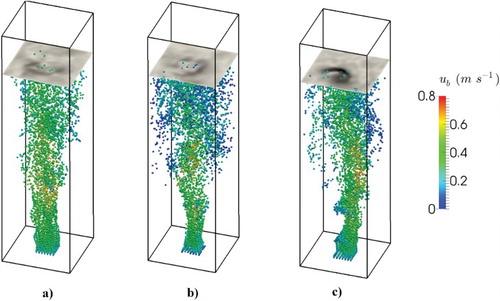
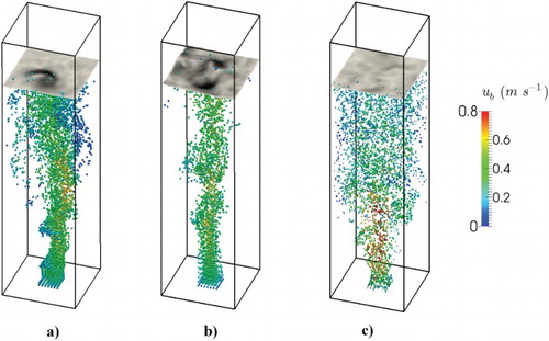
Figure 3 shows an instantaneous 3D view of bubble distribution over the investigated bubble column for the adopted drag closures. Here, it can be seen that the bubbles spread over the column for all cases, especially in the upper part of the bubble column. It is observed that the bubbles spread more in the case of drag model 2 (see, Figure 3). The bubble spread is illustrated later using the normalized bubble number concentration. Moreover, it can be seen that the bubbles exhibit lower velocity in the near-wall region. This finding is attributed to the fact that the bubbles frequently enter the downward flow regions close to the walls. This leads to a reduction in velocity of rising bubbles. As the bubbles reach the center of the bubble column, an increase in bubble rising velocity is observed.

Figure 3. Instantaneous 3D view of bubble distribution over the bubble column for the studied cases: (a) drag model 1, (b) drag model 2, (c) drag model 3.

The bubble spread in terms of the normalized bubble number concentration over line L2 is shown in Figure 4. Here, it can be seen that a nearly symmetric distribution profile is obtained in the case of drag models 1 and 3, whereas a slight asymmetric profile is observed by using drag model 2. Furthermore, it is indicated that drag model 2 yields more bubble spread in comparison with the other models. The probability that the bubbles move to the near-wall region is much higher than in the other models. Unfortunately, this quantity is not compared with experimental data because it is not provided by the experiment.

Figure 4. Bubble distribution in terms of the normalized bubble number concentration over line L2 (see Figure 2).

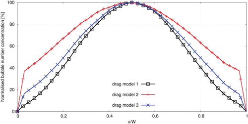
The numerical results are plotted only over line L2 because the effect of the drag model on bubble spread can be observed better in the upper part of the bubble column than in the lower part.

5.1.2. Mean velocity of liquid and bubbles

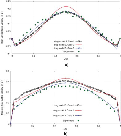
The averaged vertical velocity profile of both phases in the simulations and the experiment is compared with that obtained from the experiment in Figure 5 over line L1. Again, the present study shows a nearly symmetric profile in the case of drag models 1 and 3. On the contrary, a slightly asymmetrical profile is obtained by choosing drag model 2 in spite of the long averaging time. The maximal velocity of the liquid phase does not occur in the center of the column. Comparing the numerical and the experimental results, it can be seen that the liquid velocity is predicted well by the simulation for all drag models (see Figure 5). The maximal liquid velocity obtained from the simulation matches well with the experimental one in the case of drag model 3. On the other hand, drag model 1 overestimates the maximal velocity slightly, while it is underestimated in the case of drag model 2. Furthermore, it is obvious that the downward flow region taking place close to the walls can be determined well with the help of simulation for all used drag models. The long-term average of the simulations with drag model 1 and 3 are in line with the results from other studies used the Euler–Euler (Ma et al., 2015) and the Euler–Lagrange (Jain et al., 2014). On the contrary, the long-term average of the simulation with drag model 2 gives an asymmetrical profile with a lower maximum velocity. Additionally, none of the shown numerical results are able to resolve the profile from the experiment in full agreement.

Figure 5. Comparison between the simulated and experimental vertical velocity profile of liquid (a) and gas (b) over line L1 (see Figure 2).

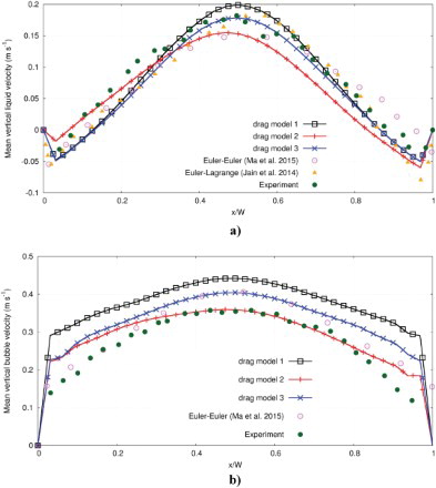
A comparison between the simulated and the experimental velocity of the bubbles over line L1 is depicted in Figure 5. Drag models 1 and 3 provide a symmetrical profile. Despite the relatively long averaging time, an asymmetric profile is achieved by drag model 2. The simulations show a noticeable deviation from the experiment for all cases. However, it can be observed that the profile slope in the case of drag models 1 and 3 agrees well with the slope of the experimental profile. Furthermore, it is clear that the velocity in the case of drag model 2 is lower compared to that obtained from other models. Drag model 2 can capture the maximal velocity detected experimentally. A comparison with the Euler–Euler simulation performed by Ma et al. (2015) shows that the vertical velocity of the bubbles is not captured in full agreement by the Euler–Euler simulation as well. The vertical velocity profiles of bubbles resulting from our simulations are not compared with the Euler–Lagrange simulation performed by Jain et al. (2014) because the authors did not provide these profiles in their paper.

5.1.3. Mean velocity fluctuations of liquid

A comparison between the simulated and experimental liquid velocity fluctuation over L1 is shown in Figure 6. The numerical vertical liquid velocity fluctuations are presented in Figure 6. Here, a comparison between the Euler–Euler (Ma et al., 2015) and Euler–Lagrange (Jain et al., 2014) simulation is depicted. It can be seen here that the Euler–Euler simulation best fits the experiment. The current simulation results show deviation compared to the experimental results. We assume that this deviation is due to our model, where the total turbulence fluctuations are not solved completely. Comparing the current numerical results, it can be seen that drag model 2 predicts higher fluctuations in the region close to the wall.

Figure 6. Comparison between the time-averaged simulated and experimental profiles of the liquid velocity fluctuations over line L1 (see Figure 2): (a) horizontal fluctuation, (b) vertical fluctuation.

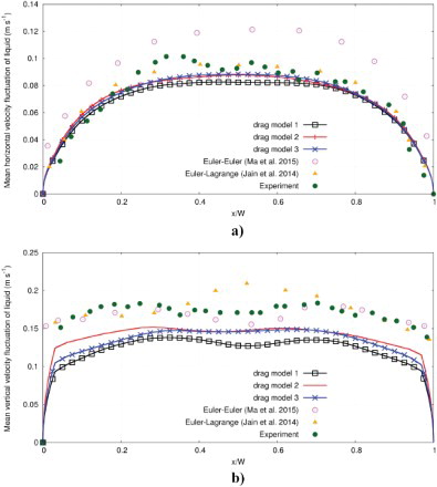
Comparing the horizontal liquid velocity fluctuation detected numerically and experimentally, a good agreement is obtained, especially in the region close to the wall (see Figure 6). Furthermore, the used drag models provide approximately a symmetric profile. On the other hand, the experiment exhibits an asymmetrical profile, which could be caused by a systematic error taking place in the experiment or by the different bubble injection conditions at the sparger. The Euler–Lagrange simulation conducted by Jain et al. (2014) predicts the horizontal fluctuations of the liquid velocity well, while the horizontal fluctuation of liquid velocity is overestimated in the Euler–Euler simulation to some extent as done by Ma et al. (2015). This is caused, according to the authors, by the high ratio of the modeled horizontal fluctuations to the total horizontal fluctuations.

5.2. Impact of injection conditions

The effects of inhomogeneous inflow conditions of the dispersed bubbles on the results are investigated in this section. Since no information about such inhomogeneous conditions is given in Deen et al. (2000), arbitrary inflow conditions are chosen here to show the effect of these conditions on the flow behavior and on bubble dynamics.

5.2.1. Impact of initial bubble velocity

The influence of injection conditions of the bubbles introduced at the sparger on the bubble dynamics and on the flow in the cavity is investigated. Therefore, the initial bubble velocity at the sparger is varied and has different values u_b = 0, 0.2, 0.3, 0.4 m/s. These values of velocity are chosen because it can be observed from the experiment that the mean vertical velocity of bubbles lies in this range (see Figure 5). Here, the bubbles are injected with a rate of n_b = 68 per hole, and drag model 3 is adopted.

Figure 7 shows that the initial velocity slightly influences the liquid velocity. Surprisingly, it is found that the maximal vertical velocity of the liquid in the case of u_b = 0.2 m/s is lower than the maximal vertical velocity in the other cases.

Figure 7. Comparison between the simulated and experimental vertical velocity profile of liquid (a) and gas (b) over line L1 (see Figure 2) to illustrate the effect of the initial velocity of the injected bubble.

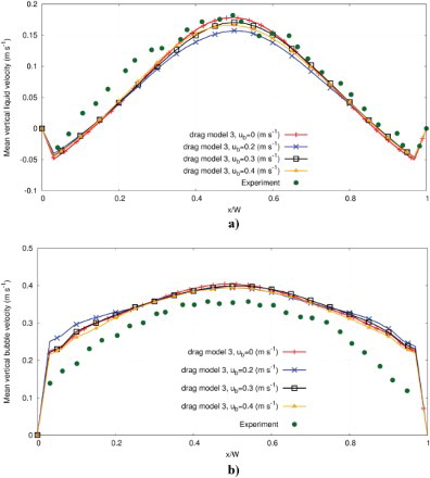
In Figure 7, it is indicated that the vertical velocity profile of bubbles is not considerably affected by the initial bubble velocity. The slope of the velocity profiles is nearly similar and unaffected by varying the initial bubble velocity as well. A slight difference is observed only in the region close to the wall.

5.2.2. Impact of bubble size distribution and bubble injection rate

The effect of bubble size distribution over the holes of the sparger and the effect of the different bubble injection rate n_b are studied. In the first case considered here, it is assumed that the bubbles are injected from each hole at the same time, and have a constant diameter of d_b = 4 mm. In this case, the bubbles are injected with n_b = 68 bubble/s (${\dot{m}}_{\mathrm{h}}$ = 2.25 cm³/s) from each hole. This case is described as Case 1 in the following paragraphs. This case is the same case studied in section 5.1. In Case 2, the bubble diameter, d_b, is kept constant, while the bubbles are injected with different n_b. Here, the bubbles are injected with a rate of n_b = 168 bubbles/s from the central sparger hole. n_b decreases by a factor of 2 to get a value of 22 bubbles/s at the outer holes. The total mass flow rate ${\dot{m}}_t$ over the sparger in Case 2 is nearly equal to ${\dot{m}}_t$ in Case 1. The distribution of n_b for Case 2 is depicted in Figure 8. In Case 3, a bubble size distribution is prescribed over the sparger. It is assumed here that the bubbles are injected with a maximal diameter (d_p = 6 mm) from the central hole of the sparger. The diameter of the injected bubbles decreases exponentially to have the minimal value at the hole at the sparger corner. The diameter distribution for Case 3 is shown in Figure 8. This diameter distribution is chosen in order to ensure that the bubble diameter in the cavity has approximately the mean bubble diameter in the experiment (d_b = 4 mm). In order to keep the mass flow rate per hole ${\dot{m}}_{\mathrm{h}}$ constant over the sparger equal to Case 1, n_b is calculated for each hole by: (19) $n_b=\frac{6{\dot{m}}_h}{\rho \pi d_b^3}.$(19) The drag model derived in Roghair et al. (2011) (drag model 3) is used in the previously considered cases. Moreover, the bubbles are initialized with u_b = 0 m/s.

Figure 8. Illustration of the different injection condition: colored circles represent the injection holes position, (a) different bubble injection rate n_b for each hole used in Case 2, (b) diameter distribution of the injected bubbles for each hole in Case 3.

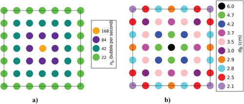
Figure 9 presents an instantaneous 3D view of the bubbles rising in the cavity. It is clear that bubble size distribution and the bubble injection rate at the sparger have a considerable impact on bubble dynamics and on bubble distribution. The bubbles spread well in Case 1 and Case 3, while the bubbles often ascend in the core region of the cavity during the simulation. The different distributions of the bubbles in these cases are attributed to the fact that the interaction between bubbles and liquid in the region close to the inlet differs between the cases. This influences the bubble distribution in the whole domain.

Figure 9. Instantaneous 3D view of bubble distribution over the bubble column for the studied cases to show the effect of the injection condition: (a) Case 1, (b) Case 2, (c) Case 3.

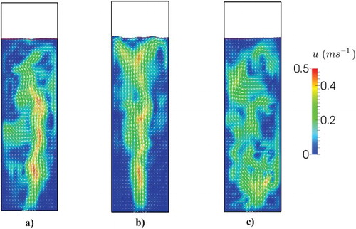
The instantaneous flow field in a mid-plane for the studied cases is shown in Figure 10. It is clear that the liquid is accelerated mainly in the core region in Case 2, especially close to the sparger region. This finding is attributed to the reason that the bubbles often stay in the core region as previously shown. On the contrary, the flow is well mixed and accelerated in the other cases, particularly in Case 3. This can be explained by the fact that the polydisperse bubbles are more dynamic and spread well in this case. Moreover, it can be seen that the fluid jet in the inlet region is not clear in comparison with Case 1 and Case 2 due to the strong mixing of the liquid in the inlet region. Moreover, the flow is dominated by many small vortices in Case 3.

Figure 10. Instantaneous snapshots of the velocity flow field for different inlet conditions: Case 1, (b) Case 2, (c) Case 3.

The significant considerable effect of the inlet condition on the time-averaged liquid and gas velocity can be seen in Figure 11. Here, it is seen that the liquid is further accelerated by the bubbles in the core region in Case 2. The maximal velocity of liquid in Case 1 and Case 3 is equal. Moreover, the velocity profile of the liquid in Case 3 matches better with the experiment.

Figure 11 Comparison between the simulated and experimental vertical velocity profile of liquid (a) and gas (b) over line L1 (see, Figure 2) to illustrate the effect of the initial velocity of the injected bubble.

Furthermore, it is observed that the velocity profiles of bubbles have different shapes (see Figure 11) due to the different bubble distribution and the different injection conditions in the studied cases. The velocity profile of bubbles in Case 3 agrees well with the experiment, practically in the side region. However, a slight overestimation of the maximal bubble velocity in Case 3 is still observed in the core region.

6. Conclusion

In the present work, the discrete bubble model (DBM) combined with the volume of fluid approach (VOF) is employed to study the hydrodynamics of a bubble column. A comparison between three drag models is indicated in the current study. These drag models are derived in Tomiyama et al. (1998), Ishii and Zuber (1979) and Roghair et al. (2011). Moreover, the present numerical results are compared with two recent studies.

It is shown that the choice of the drag closure plays a significant role for predicting the bubble dynamics and the corresponding flow behavior in the cavity. Moreover, it is seen that the consideration of the bubble swarm effect by using the Roghair drag closure enhances the flow velocity being further described.

Additionally, it is found that the bubble injection rate and bubble size distribution influence the bubbles ascending in the cavity. Moreover, they affect the flow behavior and the mean velocity profiles of both the liquid and the bubbles.

In summary, we must conclude that the actual formulation of the Euler–Lagrange model for dispersed bubbly two-phase flow still has to be improved. The implementation of the most recent drag closure models has an influence on the quality of the simulation results, but there are still some marked differences between numerically and experimentally obtained mean flow profiles.

Moreover, the definition of the more precise benchmark experiments with exact information about boundary conditions or measurement errors is also important for the proper validation of the numerical models.

In the future, possible refined models could be included in the numerical model, e.g. for bubble-induced turbulence or lift force and more precise treatment of bubble swarm effects. Additionally, a new experiment with well-defined injection conditions will be prepared for further validation of the numerical model. In this context, a grid convergence study should be performed in order to see if the results are affected by the resolution of the mesh.

Table

Symbols used
$C_D$	[-]	drag coefficient
${\mathrm{C}}_{\mathrm{D},\mathrm{\infty }}$	[-]	single bubble drag coefficient
$C_L$	[-]	lift coefficient
$C_{VM}$	[-]	virtual mass coefficient
$d_b$	[m]	bubble diameter
$Eo$	[-]	Eötvös number
$F_B$	[N ]	buoyancy force
$F_D$	[N ]	drag force
$F_G$	[N ]	gravity force
$F_L$	[N ]	lift force
$F_p$	[N ]	pressure gradient force
$F_{tot}$	[N ]	total force acting on bubble
$F_{VM}$	[N ]	virtual mass force
$F_{\sigma }$	[N m^−3]	surface tension force
g	[m s^−2]	gravitational acceleration
$M$	[N m^−3]	momentum transfer term
$p$	[N m^−2]	pressure
${Re}_b$	[-]	bubble Reynolds number
$u_f$	[m s^−1]	fluid velocity
$u_b$	[m s^−1]	bubble velocity
$u_r$	[m s^−1]	relative velocity
$V_b$	[m^3]	bubble volume
Greek symbols
$\alpha$	[-]	volume fraction in VOF
${\alpha }_{loc}$	[-]	local volume gas fraction
$\phi$	[-]	liquid property
${\nu }_{\mathrm{L}}$	[m^2 s^−1]	liquid kinematic viscosity
${\rho }_{\mathrm{L}}$	[kg m^−3]	liquid density
${\tau }^{\mathrm{model}}$	[N m^−2]	Subgrid/Reynolds stress tensor
Subscripts
B		buoyancy
$\mathrm{b}$		bubble
$\mathrm{d}$		drag
$\mathrm{f}$		fluid
G		Gravity
$\mathrm{g}$		continuous gas
$\mathrm{L}$		lift
$\mathrm{loc}$		local
$\mathrm{p}$		pressure
$\mathrm{VM}$		virtual mass

Acknowledgements

The authors would like to thank the German Science Foundation (DFG) for supporting the scientific work in terms of the Collaborative Research Centre “Multi-Functional Filters for Metal Melt Filtration-A Contribute towards Zero Defect Materials” (CRC 920 B06). Moreover, the authors acknowledge the Helmholtz Association of German Research Centers e.V. in form of the LIMTECH Alliance for supporting this research.

Disclosure statement

No potential conflict of interest was reported by the authors.

References

- Besbes, S., Hajem, M. E., Ben Aissia, H., Champagne, J. Y., & Jay, J. (2015). PIV measurements and Eulerian–Lagrangian simulations of the unsteady gas–liquid flow in a needle sparger rectangular bubble column. Chemical Engineering Science, 126, 560–572. doi: 10.1016/j.ces.2014.12.046
- Chatterjee, S., & Chattopadhyay, k. (2015). Formation of slag eye in an inert gas shrouded Tundish. ISIJ International, 55(7), 1416–1424. doi: 10.2355/isijinternational.55.1416
- Chatterjee, S., & Chattopadhyay, k. (2016). Physical modeling of slag ‘Eye’in an inert gas-shrouded Tundish using dimensional analysis. Metallurgical and Materials Transactions, 47(1), 508–521. doi: 10.1007/s11663-015-0512-x
- Chattopadhyay, K., & Guthrie, R. (2011). Considerations in using the discrete phase model. steel research international, 82(11), 1287–1289. doi: 10.1002/srin.201000214
- Clift, R., Grace, J. R., & Weber, M. E. (2005). Bubbles, drops, and particles. New York: Courier Corporation.
- Deen, N., Hjertager, B. H., & Solberg, T. (2000). Comparison of PIV and LDA measurement methods applied to the gas liquid flow in a bubble column. Proceedings of the 10th International Symposium on Applications of Laser Techniques to Fluid Mechanics, Lisbon, Portugal.
- Deen, N. G., Solberg, T., & Hjertager, B. H. (2001). Large eddy simulation of the gas–liquid flow in a square cross-sectioned bubble column. Chemical Engineering Science, 56(21), 6341–6349. doi: 10.1016/S0009-2509(01)00249-4
- Delnoij, E., Kuipers, J., & Swaaij, W. v. (1999). A three-demensional CFD model for gas-liquid bubble columns. Chemical Engineering Science, 54(13–14), 2217–2226. doi: 10.1016/S0009-2509(98)00362-5
- Delnoij, E., Lammers, F., Kuipers, J., & Swaaij, W. v. (1997). Dynamic simulation of dispersed gas-liquid two-phase flow using a discrete bubble model. Chemical Engineering Science, 52(9), 1429–1458. doi: 10.1016/S0009-2509(96)00515-5
- Deshpande, S., Anumolu, L., & Trujillo, M. (2012). Evaluating the performance of the two-phase flow solver interFoam. Computational Science & Discovery, 5(1), 14–16. doi: 10.1088/1749-4699/5/1/014016
- Dijkhuizen, W., Roghair, I., van Sint Annaland, M., & Kuipers, J. (2010). DNS of gas bubbles behaviour using an improved 3D front tracking model-drag force on isolated bubbles and comparison with experiments. Chemical Engineering Science, 65(4), 1415–1426. doi: 10.1016/j.ces.2009.10.021
- Ervin, E., & Tryggvason, G. (1997). The rise of bubbles in a vertical shear flow. Journal of Fluid Engineering, 119(2), 443–449. doi: 10.1115/1.2819153
- Grace, J., Wairegi, T., & Nguyen, T. (1976). Shapes and velocities of single drops and bubbles moving freely through immiscible liquids. Transactions of the Institution of Chemical Engineers, 54(3), 167–173.
- Greifzu, F., Kratzsch, C., Forgber, T., Lindner, F., & Schwarze, R. (2016). Assessment of particle-tracking models for dispersed particle-laden flows implemented in OpenFOAM and ANSYS FLUENT. Engineering Applications of Computational Fluid Mechanics, 10(1), 30–43. doi: 10.1080/19942060.2015.1104266
- Hirt, C., & Nichols, B. (1981). Volume of Fluid (VOF) method for the dynamics of free boundaries. Journal of Computational Physics, 39(1), 201–225. doi: 10.1016/0021-9991(81)90145-5
- Ishii, M., & Zuber, N. (1979). Drag coefficient and relative velocity in bubbly, droplet or particulate flows. AIChE Journal, 25(5), 843–855. doi: 10.1002/aic.690250513
- Jain, D., Kuipers, J., & Deen, N. (2014). Numerical study of coalescence and breakup in a bubble column using a hybrid volume of fluid and discrete bubble model approach. Chemical Engineering Science, 119, 134–146. doi: 10.1016/j.ces.2014.08.026
- Jakobsen, H., Sannaes, B., Grevskott, S., & Svendsen, H. (1997). Modeling of vertical bubble driven flows. Industrial and Engineering Chemistry Research, 36(10), 4052–4074. doi: 10.1021/ie970276o
- Klostermann, J., Schaake, K., & Schwarze, R. (2013). Numerical simulation of a single rising bubble by VOF with surface compression. International Journal for Numerical Methods in Fluids, 71(8), 960–982. doi: 10.1002/fld.3692
- Lau, Y. M., Bai, W., Deen, N. G., & Kuipers, J. (2014). Numerical study of bubble break-up in bubbly flows using a deterministic Euler–Lagrange framework. Chemical Engineering Science, 108, 9–22. doi: 10.1016/j.ces.2013.12.034
- Lau, Y. M., Roghair, I., Deen, N. G., van Sint Annaland, M., & Kuipers, J. A. (2011). Numerical investigation of the drag closure for bubbles in bubble swarms. Chemical Engineering Science, 66(14), 3309–3316. doi: 10.1016/j.ces.2011.01.053
- Ma, T., Lucas, D., Ziegenhein, T., Fröhlich, J., & Deen, N. G. (2015). Scale-adaptive simulation of a square cross-sectional bubble column. Chemical Engineering Science, 131, 101–108. doi: 10.1016/j.ces.2015.03.047
- Masood, R., & Delgado, A. (2014). Numerical investigation of the interphase forces and turbulence closure in 3D square bubble columns. Chemical Engineering Science, 108, 154–168. doi: 10.1016/j.ces.2014.01.004
- Mei, R., Klausner, J. F., & Lawrence, C. J. (1994). A note on the history force on a spherical bubble at finite Reynolds number. Physics of Fluids, 6, 418–420. doi: 10.1063/1.868039
- Miao, X., Lucas, D., Ren, Z., Eckert, S., & Gerbeth, G. (2013). Numerical modeling of bubble-driven liquid metal flows with external static magnetic field. International Journal of Multiphase Flow, 48, 32–45. doi: 10.1016/j.ijmultiphaseflow.2012.07.014
- Movahedirad, S., Ghafari, M., & Dehkordi, A. M. (2012). Discrete bubble model for prediction of bubble behavior in 3D fluidized beds. Chemical Engineering & Technology, 35(5), 929–936. doi: 10.1002/ceat.201100383
- Pan, Y., Dudukovic, M. P., & Chang, M. (1999). simulation of bubbly flow in bubble columns. Chemical Engineering Science, 54(13), 2481–2489. doi: 10.1016/S0009-2509(98)00453-9
- Pourtousi, M., Sahu, J., & Ganesan, P. (2014). Effect of interfacial forces and turbulence models on predicting flow pattern inside the bubble column. Chemical Engineering and Processing, 75, 38–47. doi: 10.1016/j.cep.2013.11.001
- Renze, P., Buffo, A., & Marchisio, D. (2014). Simulation of coalescence, breakup, and mass transfer in polydisperse multiphase flows. Chemie Ingenieur Technik, 86(7), 1088–1098. doi: 10.1002/cite.201400004
- Roghair, I., Lau, Y., Deen, N., Slagter, W., Baltussen, V. S., & Kuipers, J. (2011). On the drag force of bubbles in bubble swarms at intermediate and high Reynolds numbers. Chemical Engineering Science, 66(14), 3204–3211. doi: 10.1016/j.ces.2011.02.030
- Sankaranarayanan, K., Shan, X., Kevrekidis, I. G., & Sundaresan, S. (1999). Bubble flow simulations with the lattice Boltzmann method. Chemical Engineering Science, 54(21), 4817–4823.
- Sankaranarayanan, K., Shan, X., Kevrekidis, I. G., & Sundaresan, S. (2002). Analysis of drag and virtual mass forces in bubbly suspensions using an implicit formulation of the Lattice Boltzmann Method. Journal of Fluid Mechanics, 452, 61–96. doi: 10.1017/S0022112001006619
- Schiller, L., & Naumann, Z. (1935). A drag coefficient correlation. Verein Deutscher Ingenieure, 77(318), 51.
- Schwarz, S., & Fröhlich, J. (2013). Simulation of a bubble chain in a container of high aspect ratio exposed to a magnetic. The European Physical Journal Special Topics, 220(1), 195–205. doi: 10.1140/epjst/e2013-01807-2
- Shah, Y., Kelkar, B., Godbole, S., & Deckwer, W. (1982). Design parameters estimation for bubble column reactors. AIChE Journal, 28, 353–379. doi: 10.1002/aic.690280302
- Shalaby, H., Wozniak, k., & Gönter, W. (2008). Numerical calculation of particle-laden cyclone separator flow using LES. Engineering Applications of Computational Fluid Mechanics, 2(4), 382–392. doi: 10.1080/19942060.2008.11015238
- Shirani, E., Jafari, A., & Ashgriz, N. (2006). Turbulence models for flows with free surfaces and interfaces. AIAA Journal, 44, 1454–1462. doi: 10.2514/1.16647
- Simonnet, M. C., Gentric, C., Olmos, E., & Midoux, N. (2007). Experimental determination of the drag coefficient in a swarm of bubbles. Chemical Engineering Science, 62(3), 858–866. doi: 10.1016/j.ces.2006.10.012
- Smith, B. L. (1998). On the modelling of bubble plumes in a liquid pool. Applied Mathematical Modelling, 22(10), 773–797. doi: 10.1016/S0307-904X(98)10023-9
- Sokolichin, A., & Eigenberge, G. (1999). Applicability of the standard k-e turbulence model to the dynamic simulation of bubble columns: Part I. detailed numerical simulation. Chemical Engineering Science, 54(13), 2273–2284. doi: 10.1016/S0009-2509(98)00420-5
- Sommerfield, M., Bourloutski, E., & Bröder, D. (2003). Euler/Lagrange calculations of bubbly flows with consideration of bubble coalescence. The Canadian Journal of Chemical Engineering, 81(3–4), 508–518. doi: 10.1002/cjce.5450810324
- Spalart, P. R., Deck, S., Shur, M. L., Squires, K., Strelets, M. k., & Travin, A. (2006). A new version of detached-eddy simulation, resistant to ambiguous grid densities. Theoretical and Computational Fluid Dynamics, 20, 181–195. doi: 10.1007/s00162-006-0015-0
- Tomiyama, A., Kataoka, I., Zun, I., & Sakaguchi, T. (1998). Drag coefficients of single bubbles under normal and micro gravity conditions. JSME International Journal Series B Fluids and Thermal Engineering, 41, 472–479. doi: 10.1299/jsmeb.41.472
- Tomiyama, A., Tamai, H., Zun, I., & Hosokawa, S. (2002). Transverse migration of single bubbles in simple shear flows. Chemical Engineering Science, 57(11), 1849–1858. doi: 10.1016/S0009-2509(02)00085-4
- Tryggvason, G., Scardovelli, R., & Zaleski, S. (2011). Direct numerical simulations of gas–liquid multiphase flows. Cambridge: Cambridge University Press.
- Van der Hoef, M., van Sint Annaland, M., Deen, N., & Kuipers, J. (2008). Numerical simulation of dense gas-solid fluidized beds: A multiscale modeling strategy. Annual Review of Fluid Mechanics, 40, 47–70. doi: 10.1146/annurev.fluid.40.111406.102130
- Wörner, M. (2012). Numerical modeling of multiphase flows in microfluidics and micro process engineering: A review of methods and applications. Microfluidics and Nanofluidics, 12(6), 841–886. doi: 10.1007/s10404-012-0940-8
- Yeoh, G., & Jiyuan, T. (2009). Computational techniques for multiphase flows. Butterworth-Heinemann: Elsevier.
- Zhang, D., Deen, N., & Kuipers, J. (2006). Numerical simulation of the dynamic flow behavior in a bubble column: A study of closures for turbulence and interface forces. Chemical Engineering Science, 61(23), 7593–7608. doi: 10.1016/j.ces.2006.08.053
- Ziegenhein, T., Rzehak, R., & Lucas, D. (2015). Transient simulation for large scale flow in bubble columns. Chemical Engineering Science, 122, 1–13. doi: 10.1016/j.ces.2014.09.022
- Ziegenhein, T., Rzehak, R., Krepper, E., & Lucas, D. (2013). Numerical simulation of polydispersed flow in bubble columns with the inhomogeneous multi-size-group model. Chemie Ingenieur Technik, 85(7), 1080–1091. doi: 10.1002/cite.201200223
- Zun, I. (1980). The transverse migration of bubbles influenced by walls in vertical bubbly flow. International Journal of Multiphase Flow, 6(6), 583–588. doi: 10.1016/0301-9322(80)90053-1