Body-fin interference on the Magnus effect of spinning projectile in supersonic flows

ABSTRACT

The numerical simulations of flow over a spinning finned projectile at angles of attack ranging from $4^{\circ }$ to ${30.3}^{\circ }$ in supersonic conditions were carried out to investigate the flow mechanism of the Magnus effect. The finite volume method, a dual-time stepping method, and a $\gamma -\mathrm{R}{\mathrm{e}}_{\theta }$ transition model were combined to solve the Reynolds-averaged Navier-Stokes (RANS) equations. The validation of temporal resolution, grid independence, and turbulence models were conducted for the accuracy of the numerical method. The numerical results were in certain agreement with archival experimental data. A comparison of the transient lateral force and time-averaged Magnus force between the body of finned projectile and the nonfinned body, the projectile fin and single fin was given. The key lies in the analysis of the reasons for the production of the Magnus force. The simulation provided a profound insight into the flow structure and revealed the following. The fin leading edge shock contributes to the unsteady interference on body lateral force, while the time-averaged body Magnus force is similar to that of the nonfinned body. At $\alpha ={30.3}^{\circ }$, the shielding effect of body on crossflow weakens the time-averaged body Magnus force induced by asymmetrical flow separation, the magnitude of which is reduced to the value at $\alpha =8^{\circ }$. The leeward separation vortices and the resistance on wingroot flow are responsible for the nonlinear interference of the projectile body on fin Magnus force at different angles of attack. When the low pressure region of the vortex core is equivalent to the size and position of fin, leeward separation vortices contribute more the time-averaged Magnus force and induce high frequency variation to the transient fin lateral force.

KEYWORDS:

• Spinning projectile
• Magnus effect
• numerical simulation
• body-fin interference
• frequency analysis

1. Introduction

Many projectiles spin around their longitudinal axis during flight for advantages such as obtaining stability through the gyroscopic effect, eliminating or decreasing adverse effects caused by eccentricity, and simplifying the control system. However, spin can induce asymmetrical flow field about the angle of attack plane, causing a lateral force perpendicular to the angle of attack plane and a yawing moment, which are responsible for the trajectory dispersion. This special characteristic induced by spin is referred to as the Magnus effect. Although Magnus force is only 1/100 to 1/10 of normal force, the combination of lateral force and longitudinal force can induce the coning motion of the projectile, which significantly influences the projectile dynamic stability. For example, divergent coning motion was observed for 1/3 of the total 60 flight tests for the American Tomahawk sounding rocket (Curry & Uselton, 1967; Sturek et al., 1978). Predicting the Magnus effect accurately and investigating its flow mechanism are what researches have been longing for.

During the past few decades, the Magnus effect of nonfinned projectile has been studied by many researchers (Despirito & Plostins, 2007; Fletcher, 1972; Klatt, Hruschka, & Leopold, 2012, 2014; Nietubicz & Opalka, 1980; Silton, 2005; Simon, Deck, Guillen, Merlen, & Cayzac, 2009). The previous work indicates that the boundary layer distortion is the main source of the Magnus effect at small angles of attack, and that the asymmetrical flow separation on the projectile surface directly influences the Magnus effect at large angles of attack. The configuration of a nonfinned projectile is relatively simple and the Magnus effect induced by spin has quasi-steady characteristic. Thus, the Magnus effect of a nonfinned projectile in supersonic flows can be calculated using steady algorithm with the addition of a moving surface boundary condition, and good results are obtained compared with experimental data. Different from the quasi-steady Magnus effect of nonfinned projectile, the lateral force and yawing moment of finned projectile change with time and have obvious unsteady characteristics (Cayzac, Carette, Denis, & Guillen, 2011).

Essentially, the lateral force of a spinning finned projectile is composed of two parts: one for the asymmetrical configuration at different rolling angles, and the other for the additive effect induced by spin, which is called the Magnus effect. For an initial configuration symmetrical about angle of attack plane, within a rotation period, the transient lateral force of the former term can be considerable while the time-averaged effect is zero; meanwhile, the transient lateral force of the latter term is small while the time-averaged Magnus force is nonzero. Therefore, the transient force perpendicular to the angle of attack plane at different rolling angles is referred to as the lateral force, and its time-averaged value is referred to as the Magnus force.

Earlier studies on the Magnus effect over a spinning finned projectile were usually carried out using theoretical and experimental methods. Platou (1965) pointed out that the aerodynamic load on the leeward fin was reduced at nonzero angles of attack, causing an opposite Magnus force on the fins compared with that on the body. The research of Benton (1962) indicated that Magnus moment could be produced by canted fins in supersonic flows. The predicted values obtained from the Magnus moment coefficient derivative formula given by Benton (1964) were in good agreement with experimental data at high Mach numbers, while large errors occurred when Mach number was lower than 1.4 due to body-fin interference. The influence of separation vortices on the fin Magnus force was studied by Oberkampf and Nicolaides (1971) using potential flow theory. The Magnus force and moment of finned projectile with control surfaces in subsonic and transonic velocities were investigated by Seginer and Rosenwasser (1986) through experiment, and the change in the direction of the Magnus effect was discovered. Theoretical methods are usually used for single aerodynamic component, such as single fin and nonfinned body, and it is hard to describe the interference and three-dimensional effect between aerodynamic components. Moreover, wind tunnel tests measure the aerodynamic characteristics of the whole projectile, while the relationships between unsteady flow structures and aerodynamic characteristics are difficult to determine.

(Despirito & Plostins, 2007; Fletcher, 1972; Klatt et al., 2012, 2014; Nietubicz & Opalka, 1980; Silton, 2005; Simon et al., 2009).

With the development of computational technology, computational fluid dynamics (CFD) methods, such as steady and unsteady simulations, RANS simulations based on different turbulence models, and direct numerical simulations, are frequently used to predict total aerodynamic coefficients, dynamic derivatives, and complex flow phenomena (Hu, Li, Han, Steve, & Xu, 2016; Seyfert & Krumbein, 2012; Zhang, Wang, Liang, & Liu, 2015). So far, the numerical investigations on the Magnus effect of spinning finned projectile are slight. Researches of the Magnus effect at small angles of attack ($\alpha <{4.2}^{\circ }$) were carried out by Pechier, Guillen, and Cayzac (2001). The results showed that the fin Magnus force was dominant and had opposite direction to the body Magnus force. The total aerodynamic coefficients and dynamic derivatives of finned projectile were computed in supersonic flows from 0 to 90 degrees angle of attack by Bhagwandin using $k-\epsilon$ turbulence model (2012). The former study had certain limitations because the interference between the body and the fin was relatively small at small angles of attack and flow separation was not taken into consideration. The latter was concentrated on the computation of aerodynamic coefficients while the insight of flow field structures was not involved in. Dealing the complete three-dimensional (3D) unsteady RANS equations is computationally expensive, thus, it is necessary to choose the appropriate computational methods and turbulence models. In a word, the aforementioned studies neither include the comparison of the Magnus effect of a spinning finned projectile using different turbulence models, nor the analysis of the corresponding flow structures and the distribution characteristics of lateral force.

In this paper, to the authors’ knowledge, the $\gamma -\mathrm{R}{\mathrm{e}}_{\theta }$ transition model and different fully turbulence models were used for the first time to calculate the aerodynamic characteristics and simulate the flow field structure over spinning finned projectile in supersonic flows at angles of attack from $4^{\circ }$ to ${30.3}^{\circ }$. Better results were obtained by the $\gamma -\mathrm{R}{\mathrm{e}}_{\theta }$ transition model compared with experimental data. A comparison of the transient lateral force and the time-averaged Magnus force between the body of finned projectile and the nonfinned body, the projectile fin and single fin was made to analyze the interference between the aerodynamic components. The key lies in the reveal of physical origins, such as fin leading edge shock and leeward separation vortices, for the production of Magnus force. The profound insight of the relationship between aerodynamic characteristics and flow structure can provide guidance for the design of projectile configuration and control system.

2. Numerical approach

2.1. Governing equations and turbulence models

The integral form of the three-dimensional Navier-Stokes equations was used as governing equations for fluid flow, which is combined with dual-time stepping method:

(1) $\begin{array}{rl}& \frac{\mathrm{\partial }}{\mathrm{\partial }t}{\int }_V\mathbf{\text{W}}\mathrm{d}V+\mathrm{\Gamma }\frac{\mathrm{\partial }}{\mathrm{\partial }\epsilon }{\int }_V\mathbf{\text{Q}}\mathrm{d}V+\oint [\mathbf{\text{F}}-\mathbf{\text{G}}]\cdot \mathrm{d}\mathbf{\text{A}}\\ & ={\int }_V\mathbf{\text{H}}\mathrm{d}V\end{array}$(1) (2) $\begin{array}{rl}\mathbf{\text{W}}& =\left\{\begin{array}{c}\rho \\ \rho u\\ \rho v\\ \rho w\\ \rho E\end{array}\right\},\mathbf{\text{Q}}=\left\{\begin{array}{c}p\\ u\\ v\\ w\\ T\end{array}\right\},\mathbf{\text{F}}=\left\{\begin{array}{c}\rho \mathit{v}\\ \rho \mathit{v}u+p\mathit{i}\\ \rho \mathit{v}v+p\mathit{j}\\ \rho \mathit{v}w+p\mathit{k}\\ \rho \mathit{v}E+p\mathit{v}\end{array}\right\},\\ \mathbf{\text{G}}& =\left\{\begin{array}{c}0\\ {\tau }_{xi}\\ {\tau }_{yi}\\ {\tau }_{zi}\\ {\tau }_{ij}{v}_j+f\end{array}\right\}\end{array}$(2) where H, F, and G denote the source, convection, and viscous term, respectively. V is control volumn. $\mathit{v}$ denotes the velocity vector, and variables u, v, and w are the velocity components in x, y, and z direction, respectively. $\rho$, P, and T are density, pressure, and temperature, respectively. $\epsilon$ is pseudo-time in the time-marching procedure, and $\mathrm{\Gamma }$ is the preconditioning matrix. In the equations above, E, $\tau$, and f are used to represent total energy per unit mass, the viscous stress tensor, and the heat flux, respectively. Meanwhile, E can be expressed as: (3) $E=h+\frac{V^2}{2}-\frac{P}{\rho }$(3) where h is enthalpy, and V is velocity magnitude. Moreover, the ideal gas state equation is necessary for a closed system: (4) $P=\rho RT$(4) where R is gas constant and $R=287\mathrm{J}/(\mathrm{kg}\cdot \mathrm{K})$. For the dependence of viscosity on temperature, Sutherland’s law was used: (5) $\mu ={\mu }_0{\left(\frac{T}{T_0}\right)}^{\frac{3}{2}}\frac{T_0+S}{T+S}$(5) where $T_0=275\mathrm{K}$, ${\mu }_0=1.71\times {10}^5\mathrm{kg}\cdot {\mathrm{m}}^{-1}$, and S = 110 K.

For turbulent flows, a Reynolds-averaged form of these equations were used, and the above equations were solved using an implicit solver based on the finite volume method. The second order upwind scheme was used for spatial discretization. The dual-time stepping method consists of a physical time step describing the model motion and an inner time step used to converge the RANS equations (DeRango & Zingg, 1997; Pandya, Venkateswaran, & Pulliam, 2003). At each physical time step, the flow variables are determined by the flow state at the previous time step and the inner pseudo-time iteration.

A steady state simulation without spin was first carried out to get converged flow field, which was then used as an initial state for unsteady simulation to rapidly and stably obtain converged results. The solution was regarded converged when the flow residuals dropped at least three orders of magnitude and the aerodynamic coefficients varied within 0.1%. Temporal and grid resolution studies were conducted for the accuracy of the numerical method. Meanwhile, the results obtained from different turbulence models, including Spalart-Allmaras (Spalart & Allmaras, 1992), $k-\epsilon$ (Shih, Liou, Shabbir, Yang, & Zhu, 1995), $k-\omega$ (Menter, 1994), and $\gamma -\mathrm{R}{\mathrm{e}}_{\theta }$ (Menter et al., 2004a, 2004b) transition model, were compared. The $\gamma -\mathrm{R}{\mathrm{e}}_{\theta }$ transition model, combining the robustness and accuracy of the $k-\omega$ model at the near wall region, the freestream independence of the $k-\epsilon$ at far field, and the transport equations of intermittency and transition, was expected to capture effectively the boundary layer flow and complex flow phenomenon.

The influence of different flow structures on the aerodynamic characteristics of vehicles is reflected by the wall surface pressure and shear stress. From the view of numerical calculation, the pressure perpendicular to and the viscous force tangential to the projectile surface can be obtained after solving the Reynolds-averaged Navier-Stokes equations. Projecting all forces towards the z axis direction (perpendicular to the angle of attack plane), and then integrating the values at all surface girds together, the projectile total lateral force can be obtained. Similarly, the lateral force of the projectile body and fin can be calculated by integrating the force at body surface grids and fin surface grids, respectively. However, the contribution of viscous force on the lateral/Magnus force is usually 1/100 to 1/10 compared with that of pressure, only the pressure term is chosen for detailed analysis in this paper.

2.2. Computational model and conditions

The Air Force Modified Basic Finner Projectile (AFF) was used for numerical simulations, and its configuration and dimension are shown in Figure 1. The diameter of the projectile body is d = 45.72 mm (1-caliber). The projectile consists of a 2.5-cal. ogive nose, a 7.5-cal. cylinder body, and four symmetrical uncanted fins. The moment reference point is 5-cal. from the nose vertex. The reference length and area are L_ref = 0.04572 m and S_ref = 0.00164 m², respectively. The experimental conditions were Mach number Ma = 2.5, Reynolds number based on model diameter $\mathrm{R}{\mathrm{e}}_d=2.6\times {10}^5$, total pressure $P_0=61360\mathrm{Pa}$, total temperature $T_0=311\mathrm{K}$, angle of attack $\alpha ={4.0}^{\circ }\sim {30.3}^{\circ }$, and non-dimensional spin rate $\overline{\omega }=\omega d/\left(2V_{\mathrm{\infty }}\right)=0.025$. The corresponding freestream conditions were $P_{\mathrm{\infty }}=3624.5\mathrm{Pa}$, $T_{\mathrm{\infty }}=137.66\mathrm{K}$, ${\rho }_{\mathrm{\infty }}=0.092\mathrm{kg}/{\mathrm{m}}^3$, $V_{\mathrm{\infty }}=588\mathrm{m}/\mathrm{s}$, and spin rate $\omega =642\mathrm{rad}/\mathrm{s}$.

Figure 1. Model configuration and dimension.

2.3. Computational grid and boundary conditions

A 3D structured hexahedral mesh is shown in Figure 2. The Magnus effect is closely related to the near wall flow. Therefore, the viscous sublayer should be adequately resolved and the height of the first layer gird was set to $5\times {10}^{-6}\mathrm{m}$, ensuring that non-dimensional wall distance $y^{+}\le 1$. The stretching ratio of the first 15 grid layers was kept to 1.1. The far field was located two times the projectile length away from the projectile nose and the circumferential body. The outlet boundary was located a projectile length downstream from the base, allowing shocks to leave without reflecting at the boundary and contaminating the flow field. The projectile surface was set to no-slip, adiabatic, and stationary wall condition. To exclude the influence of grid on the results, three sets of mesh were generated for the grid resolution study. The specific grid parameters around the projectile surface are shown in Table 1. The coordinate system, fixed and do not spin with the projectile, is shown in Figure 2. The projectile was experiencing a counterclockwise spin about its longitudinal axis from the view of the projectile base.

Figure 2. Computational grid.

Table 1. Computational grid parameters.

	Coarse	Medium	Fine
Axial (body)	210	265	340
Spanwise	36	46	56
Circumferential	120	156	196
Total (Mil.)	3.96	7.38	11.27

3. Validation of numerical approach

3.1. Temporal resolution

The computational conditions at $\alpha ={20.2}^{\circ }$ and $\overline{\omega }=0.025$ were used for a time step independence study. The medium grid and the $\gamma -\mathrm{R}{\mathrm{e}}_{\theta }$ transition model were used to exclude the influence of grid and transition model. 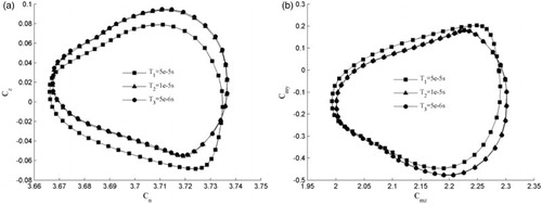Three physical time steps were set to $T_1=5\times {10}^{-5}\mathrm{s}$, $T_2=1\times {10}^{-5}\mathrm{s}$, and $T_3=5\times {10}^{-6}\mathrm{s}$, and the corresponding spin angles were 1.839°, 0.368°, and 0.184°. The inner iteration step was set to 20 (Bhagwandin, 2012). Figure 3 shows the aerodynamic coefficients obtained within a spin cycle using different time steps. C_n and C_z are normal force coefficient and lateral (Magnus) force coefficient, respectively. C_n = F_n/qS_ref, where F_n is the force pointing to y axis direction, and q is dynamic pressure ($q=\rho V_{\mathrm{\infty }}^2/2$). Similarly, C_z = F_z/qS_ref, where F_z is the force pointing to z axis direction. C_mz and C_my are pitching moment coefficient and yawing (Magnus) moment coefficient, respectively. Here, C_mz = M_mz/qS_refL_ref and C_my = M_my /qS_refL_ref. It can be seen that the time-averaged values of normal force and pitching moment are similar at different time steps, with relative differences being less than 0.5%. However, the Magnus force and moment coefficients are small quantities, and the results obtained using T₁ have an obvious gap compared with those obtained using T₂ and T₃. The results obtained using T₂ and T₃ are in good agreement, so the temporal resolution can be ensured using T₂.

Figure 3. Aerodynamic coefficients within a spin cycle under different time steps for (a) Normal and lateral force and (b) Pitching and yawing moment.

3.2. Grid independence

A grid independence study was carried out using the $\gamma -\mathrm{R}{\mathrm{e}}_{\theta }$ transition model and the three types of grid aforementioned. The computational conditions were $\alpha ={20.2}^{\circ }$, T₂ = $T_2=1\times {10}^{-5}$s, and $\overline{\omega }=0.025$. Table 2 gives the relative difference of aerodynamic coefficients using different grids. The results of normal force and pitching moment from different grids are similar, with relative differences being less than 0.5%. The relative difference in the time-averaged values of the Magnus force coefficient among different grids is within 8%. Therefore, the coarse mesh was considered to accurately and effectively simulate the presented problem.

Table 2. Relative difference of aerodynamic coefficients.

Difference (%)	Cn	Cz	Cmz	Cmy
Coarse-Medium	−0.06	4.02	−0.26	1.78
Coarse-Fine	−0.10	7.25	−0.29	0.28
Medium-Fine	−0.04	3.11	−0.03	−1.47

3.3. Choice of turbulence model

The variations of time-averaged Magnus force and moment coefficients with angle of attack obtained by different turbulence models are shown in Figure 4 ($\overline{\omega }=0.025$). The numerical results were compared with the archival experimental data obtained by Arnold Engineering and Development Center (AEDC) at Arnold Air Force Base (Jenke, 1976). The results from the $\gamma -\mathrm{R}{\mathrm{e}}_{\theta }$ transition model are the nearest to experimental data at $\alpha ={12.6}^{\circ }$ and $\alpha ={20.2}^{\circ }$. The boundary layer trip was not used in the experiment, so it can be deduced that the transition from laminar to turbulent flow has important effect on the Magnus effect.

Figure 4. Variation of time-averaged Magnus coefficients with angle of attack for (a) Magnus force and (b) Magnus moment.

Although a small gap lies between experimental data and the $\gamma -\mathrm{R}{\mathrm{e}}_{\theta }$ model results, their variation tendencies with angle of attack are in good agreement. In Figure 4(a), the results of other turbulence models at $\alpha ={12.6}^{\circ }$ are negative, except for that of the $\gamma -\mathrm{R}{\mathrm{e}}_{\theta }$ model. The time-averaged Magnus force of finned projectile is positive, that is, the force direction points to the positive direction of z axis, which is quite the opposite compared with the nonfinned projectile. Meanwhile, the computed normal force and pitching moment coefficients obtained by $\gamma -\mathrm{R}{\mathrm{e}}_{\theta }$ transition model match well with experimental data, with relative differences being less than 5%. It can be concluded that the flow over spinning finned projectile under supersonic conditions within certain angles of attack can be effectively and reliably simulated using the coarse mesh, the time step T₂ = $T_2=1\times {10}^{-5}\mathrm{s}$s, and the $\gamma -\mathrm{R}{\mathrm{e}}_{\theta }$ transition model.

The magnitudes of axial force and normal force are larger compared with that of lateral force. Similarly, the comparison between the CFD results and experimental data is made. The time-averaged axial and normal forces obtained by $\gamma -\mathrm{R}{\mathrm{e}}_{\theta }$ transition model at different angles of attack are shown in Figure 5. The three curves in the figure indicate the non-spin result, the time-averaged spin result ($\overline{\omega }=0.004$), and the experimental spin data, respectively. It can be seen that the relative differences between the results of spin and non-spin conditions are within 5%. Meanwhile, the calculated values are in good agreement with the experimental values. In conclusion, spin has little effect on the axial force and normal force.

Figure 5. Time-averaged coefficients at different angles of attack for (a) axial force and (b) normal force.

4. Results and discussion

4.1. Time-averaged forces at different Mach numbers

The time-averaged axial, normal, and lateral force coefficients at different Mach numbers and angles of attack are shown in Figure 6. Axial force increases first and then decreases with Mach number, reaching the maximum values at transonic speeds. This is similar to normal force. The variation amplitude of axial force at different Mach numbers is obvious, while similar values are observed at different angles of attack. The case for normal force is quite the opposite. As for lateral force, its values turn from negative to positive as Mach number increases, reaching the maximum absolute values at transonic speeds. The calculated values are in good agreement with the experimental data in supersonic conditions, while the situation in subsonic condition is not satisfied. Despirito and Plostins (2007) calculated the Magnus effect of a nonfinned projectile in subsonic speeds using hybrid RANS/LES method, and the results were improved to some extent. Therefore, the flow structure analysis about the Magnus effect is carried out only for Ma = 2.5 hereinafter.

Figure 6. Time-averaged coefficients for (a) axial force, (b) normal force, and (c) lateral force.

4.2. Transient lateral force and time-averaged Magnus force at angles of attack

Figure 7 shows the variation of lateral force and yawing moment coefficients with rolling angle $\varphi$ at different angles of attack. The curves in Figure 7 change periodically with rolling angle and their variation periods are the same as the fin number. As angle of attack increases, the absolute values of time-averaged Magnus force and moment coefficients increase. However, the transient amplitude increases first and then decreases, reaching a maximum value at $\alpha ={12.6}^{\circ }$. The direction of transient lateral force changes with rolling angle except when $\alpha ={30.3}^{\circ }$. Next, the lateral force coefficient of the finned projectile is divided into two components, the body and the fins, such as C_z-body and C_z-Fins.

Figure 7. Variation of coefficients with rolling angle for (a) lateral force and (b) yawing moment.

The variations of the body and the fins lateral force coefficients at different angles of attack are given in Figure 8. In Figure 8(a), the body lateral force presents periodical change with rolling angle due to the fin interference, which is no longer similar to the quasi-steady lateral force of the nonfinned projectile. The variation period within a rotation cycle is the same as the fin number. However, different from Figure 7(a), the amplitude of the body lateral force increases with angle of attack, and the direction changes only when $\alpha ={20.2}^{\circ }$ and $\alpha ={30.3}^{\circ }$. In turn, the fins' lateral force can be influenced by the projectile body. In Figure 8(b), the periodical variation of fins lateral force is mainly caused by the fin effective angle of attack at different rolling angles, and the body interference also influences its magnitude. It can be seen that the body and fins lateral force reach the extreme values simultaneously.

Figure 8. Variation of lateral force coefficient with rolling angle for (a) body and (b) fins.

The fins of AFF model are uniformly distributed in circumferential direction, and the force acted on each fin has the same variation tendency with only a phase difference of $\pi /2$. Fin 1, initially located in the positive y direction, is chosen for detailed analysis. Figure 9 shows the variation of Fin 1 lateral force with rolling angle. It can be seen that the amplitude of the curve increases with angle of attack. Besides, the oscillation number of curves also increases when $\alpha \ge {12.6}^{\circ }$, for example when $\varphi \in (0^{\circ },{90}^{\circ })$ and $\varphi \in ({270}^{\circ },{360}^{\circ })$.

Figure 9. Variation of Fin 1 lateral force with rolling angle.

Figure 10 presents the time-averaged Magnus force coefficients of body and Fin 1, which are separately compared with that of the nonfinned projectile and the single fin. In Figure 10(a), although the transient flow field structures around the body can be influenced by the fin, the time-averaged body Magnus force is hardly affected. The relative difference between the time-averaged body Magnus force and that of the nonfinned projectile is less than 10%. Moreover, the body Magnus force increases first and then decreases with angle of attack. Klatt et al. (2014) proposed that the generation and distortion of the secondary vortices are responsible for this phenomenon. However, the angle of attack was limited in 16°, and the rapid decrease of the Magnus force at large angle of attack was not explained. In Figure 10(b), the Fin 1 Magnus force is obviously larger than that of the single fin, that is, the interference of the body enhances the Fin 1 Magnus force and this effect increases with angle of attack. Here, at small and medium angle of attack, the magnitude of the fin Magnus force is equivalent to that of the body, and the total Magnus effect is not obvious. With the increase of angle of attack, the contribution of the fin on total Magnus force is becoming dominant.

Figure 10. Time-averaged Magnus force coefficient for (a) body vs. nonfinned projectile and (b) Fin 1 vs. single fin.

4.3. Fluctuation of body and fin transient lateral force

According to the characteristics of disturbance propagation in supersonic flow, it is known that the influence of disturbance on the flow field is limited in the Mach cone, that is, the influence of the fins on the body is limited to the body near the fins. The moment at $\varphi ={24.2}^{\circ }$, $\varphi ={64.7}^{\circ }$, and $\varphi ={88.6}^{\circ }$ in Figure 8(a) is chosen for analysis, which correspond to the negative, positive, and zero lateral force state, respectively. The transient fins interference on the body is analyzed by comparing the circumferential surface pressure distribution of the nonfinned projectile with that of the finned projectile. Figure 11 is a schematic of the profile at x/L = 0.962 when $\varphi ={24.2}^{\circ }$, where x is the projectile longitudinal coordinate and L is the projectile length. The different parts of the body and the fins are named separately.

Figure 11. Schematic of the profile at x/L = 0.962 when $\alpha ={24.2}^{\circ }$.

Figure 12 gives the circumferential surface pressure distribution of the nonfinned and the finned projectile in z direction at x/L = 0.962. In the figures, $\xi$ means circumferential position, C_p means pressure coefficient (C_p = P/$P_{\mathrm{\infty }}$), and the superscript z means the projection of C_p in z direction. For the nonfinned projectile, the pressure distribution is continuous. In Figure 12(a), the circumferential pressure distribution of the finned projectile, although interrupted near Fin 2 and Fin 4, is relatively consistent with that of the nonfinned projectile. With the increase of angle of attack, the crossflow velocity increases. In Figure 12(b), the interference of fins on body strengthens and the gap of pressure distribution around the fins increases. Meanwhile, taking the $\varphi ={24.2}^{\circ }$ case for example, the difference of circumferential pressure distribution at different body sections is obvious, and jump exists around $\xi ={135}^{\circ }$ and $\xi ={280}^{\circ }$. Detailed investigation is conducted through the flow field structure analysis.

Figure 12. Circumferential pressure coefficient distribution in z direction at x/L = 0.962 for (a) $\alpha ={4.0}^{\circ }$ and (b) $\alpha ={20.2}^{\circ }$.

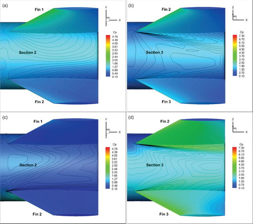
The pressure coefficient contours of body and fins at $\varphi ={24.2}^{\circ }$ is shown in Figure 13. From Figure 13(a) and (c), it can be seen that the pressure coefficient at small angle of attack is obviously higher than the case at large angle of attack, which is mainly caused by the resistance of fins on crossflow. Section 2 is not influenced by fin leading edge shock, and the corresponding curves in Figure 12(a) are relatively smooth. From Figure 13(b) and (d), it can be seen that the pressure coefficient at $\alpha ={4.0}^{\circ }$ is lower than that at $\alpha ={20.2}^{\circ }$. Moreover, the pressure distribution is influenced by fin leading edge shock, and this is the reason for the curve jump around $\xi ={135}^{\circ }$ in Figure 12(b). No additional influence is produced by the shock interference.

Figure 13. Pressure coefficient contours of body and fins at $\alpha ={24.2}^{\circ }$ for (a) $\alpha ={4.0}^{\circ }$ Section 2, (b) $\alpha ={4.0}^{\circ }$ Section 3, (c) $\alpha ={20.2}^{\circ }$ Section 2, and (d) $\alpha ={20.2}^{\circ }$ Section 3.

The body and fin transient lateral forces reach the extreme values simultaneously according to Figure 8. The maximum fin lateral force state (Figure 11) was chosen to analyze the body interference on fin. The Fin 1 pressure distribution was compared with that of the single fin. The fin spanwise distribution of pressure difference between windward and leeward in z direction at x/L = 0.962 is shown in Figure 14. As can be seen from Figure 14(a), for the single fin, the surface pressure difference in z direction increases with angle of attack and shows large variation at midspan due to wingroot effect; for Fin 1, the surface pressure difference in z direction shows no regular variation with angle of attack, and even points to the opposite direction at $\alpha ={12.6}^{\circ }$. The gap between the pressure difference of single fin and Fin 1 increases with angle of attack, and pressure drop exists near the wingtip except for the case at $\alpha ={12.6}^{\circ }$. In Figure 14(b), the contribution of pressure difference on the fin lateral force and its gap increases with angle of attack. The pressure difference of Fin 2 is higher than that of the single fin, and the wingtip pressure drop also exists. In general, the influence of body on fin lateral force is slight at a small angle of attack. With the increase of angle of attack, the interference of projectile body induces an opposite lateral force on the leeward fin and increases the lateral force on the windward fin.

Figure 14. Spanwise pressure difference in z direction at x/L = 0.962 for (a) Fin1 vs. single fin and (b) Fin2 vs. single fin.

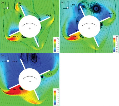
Figure 15 shows the pressure contours and streamlines at x/L = 0.962 at three angles of attack. With the increase of angle of attack, the windward pressure increases and the leeward pressure decreases. Meanwhile, the leeward separation phenomenon becomes obvious and the separation vortices shift towards positive y direction. The variation of pressure distribution of Fin 1 in Figure 14(a) shows no regular change with angle of attack because of the dramatic variation of leeward flow field structure. When $\alpha ={4.0}^{\circ }$, the flow separation is weak and has little influence on Fin 1. When $\alpha ={12.6}^{\circ }$, Fin 1 enters the left separation vortex, and the windward pressure is lower than the leeward pressure, causing the shift in lateral force direction. When $\alpha ={30.3}^{\circ }$, the leeward separation vortices shift towards positive y direction and the influence of their low-pressure center on Fin 1 decreases. For Fin 2, due to the resistance of body on the wingroot flow, the pressure difference between windward and leeward is higher compared with that of the single fin. Flow curls upward from windward to leeward due to the addition of crossflow velocity and spin rate, thus developing the wingtip vortex and weakening the fin lateral force slightly. However, for Fin 4, no wingtip vortex develops because of the counteraction between crossflow velocity and spin rate.

Figure 15. Pressure contours and streamlines at x/L = 0.962 for (a) $\alpha ={4.0}^{\circ }$, (b) $\alpha ={12.6}^{\circ }$, and (c) $\alpha ={30.3}^{\circ }$.

The flow field structure shown in Figure 15 is used to analyze the reason for the increase of the oscillation number in Figure 9, which is mainly reflected at $\varphi \in (0^{\circ },{90}^{\circ })$ and $\varphi \in ({270}^{\circ },{360}^{\circ })$. The reason is that the fin comes across the leeward wake vortices. The first set of the extreme values corresponds to the motion of the fin crossing the left separation vortex. The second set of the extreme values, also the maximum and the minimum values, indicates that the fin experiences peak forces in windward and is free of leeward separation vortices. The case for the fin’s crossing the right vortex is similar to that for the left vortex.

4.4. Decrease of body Magnus force at large angle of attack

Figure 16 illustrates the distribution of time-averaged Magnus force coefficient along projectile longitudinal axis. It can be seen that the results of the nonfinned projectile and that of the body of finned projectile are similar. When $\alpha \le {12.6}^{\circ }$, the local Magnus force increases with angle of attack and mainly acts on the afterbody. When $\alpha ={30.3}^{\circ }$, the distribution of Magnus force at the afterbody shifts dramatically, which is close to the case at $\alpha =4^{\circ }$.

Figure 16. Distribution of time-averaged body Magnus force coefficient along x axis.

The profile at x/L = 0.656 in Figure 16 is chosen for flow structure analysis. Figure 17 presents the density contours and streamlines at x/L = 0.656 under different angles of attack. The pattern of flow separation changes with angle of attack. Asymmetrical effect is not obvious due to the low dimensionless spin rate. For the left-side body, flow separation occurs earlier than the right-side body because the crossflow cannot overcome the viscous drag produced by the spinning wall. For the right-side body, separation point shifts along y axis due to the compensation of spinning wall on the adverse pressure gradient. When $\alpha ={4.0}^{\circ }$, the right-side separated flow reattached, and the separation effect is not obvious. When $\alpha ={12.6}^{\circ }$, the secondary vortices form because of the interaction between the leeward separated vortices and the near wall separated flow. When $\alpha ={30.3}^{\circ }$, the crossflow velocity increases and the separation points on both sides shift to the leeward. Moreover, the near wall vortices in Figure 17(b) merge with each other, and the projectile leeward becomes low pressure state.

Figure 17. Density contours and streamlines at x/L = 0.656 for (a) $\alpha ={4.0}^{\circ }$, (b) $\alpha ={12.6}^{\circ }$, and (c) $\alpha ={30.3}^{\circ }$.

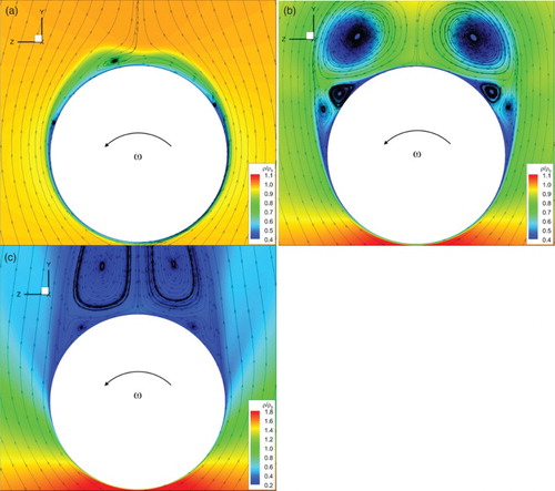
Figure 18 shows the z direction pressure difference between the right and left side bodies at x/L = 0.656. When $\alpha ={12.6}^{\circ }$, the secondary vortices induce positive contribution to the Magnus force around $\xi ={30}^{\circ }$ and $\xi ={60}^{\circ }$, however, the asymmetrical flow separation around $\xi ={100}^{\circ }$ has a more significant negative influence on the Magnus force. When $\alpha ={30.3}^{\circ }$, the leeward body is in low pressure state, thus weakening the contribution of asymmetrical flow separation on the Magnus force.

Figure 18. Distribution of circumferential pressure difference in z direction at x/L = 0.656.

4.5. Nonlinear interference of body on fin Magnus force

The fin lateral force can be obtained by projecting the normal force predicted by the effective angle of attack in z direction. The effective angle of attack ${\alpha }_e$ at $\varphi =\pm {90}^{\circ }$ can be expressed as (6) ${\alpha }_e=\alpha \pm \omega y/V_{\mathrm{\infty }}$(6) the former on the right is angle of attack, and the latter is additional angle of attack produced by spin. Now, the fin normal force reaches the extreme values.

The fin normal force is written as (7) $\begin{array}{rl}{F}_n& ={\int }_{d/2}^{d}q{C^{\mathrm{\prime }}}_{n\alpha }{\alpha }_{e}c\left(y\right)\mathrm{d}y\\ & =q{C^{\mathrm{\prime }}}_{n\alpha }(0.00104\alpha \pm 3.44\times {10}^{-5}\omega /V_{\mathrm{\infty }})\end{array}$(7) where c means the wing chord length, $c\left(y\right)=C-(y-d/2)/\tan \theta$, and the leading edge sweepback angle $\theta ={36.9}^{\circ }$. According to the rectangular fin normal force coefficient derivative formula proposed by Harmon (1949), $C_{n\alpha }=4(1-0.5AB)/B$, where A is fin aspect ratio, and $B=(\mathrm{M}{\mathrm{a}}^2-1{)}^{1/2}$, $C_{n\alpha }=0.7811$ is obtained by choosing the centroid chord length. Therefore, the dimensionless lateral force coefficient can be written as (8) $C_z=-\cos \left(\varphi \right)(0.7771\alpha \sin (\varphi )+0.0257\omega /V_{\mathrm{\infty }})\left(8\right)$(8)

Figure 19 illustrates the single fin Magnus force coefficient and the curves obtained by Equation (8) at different angles of attack. The time-averaged values of Equation (8) are zero because the influence of body and vortices is not taken into consideration. At $\alpha =8^{\circ }$, the two curves are close to each other, and their time-averaged values are approximate to zero. Certain gap exists between the two curves due to the flow separation, wingtip, and wingroot effect at $\alpha ={20.2}^{\circ }$. Predicting the transient fin lateral force through effective angle of attack is meaningful to some extent, however, the asymmetrical time-averaged effect induced by 3D unsteady flow phenomena cannot be explained.

Subtracting the single fin lateral force coefficient (Figure 19) from the Fin 1 lateral force coefficient (Figure 9), and then dividing by the maximum value of curves in Figure 9, we obtain the difference of lateral force between Fin 1 and single fin at different angles of attack, as shown in Figure 20(a). Except for the case at $\alpha ={4.0}^{\circ }$, the influence of body interference on the fin lateral force is positive when $\varphi \in (0^{\circ },{180}^{\circ })$ and is negative when $\varphi \in ({180}^{\circ },{360}^{\circ })$. Hence, the interference of body increases the fin lateral force when the crossflow velocity and spin rate have opposite directions, vice versa. Moreover, the contribution of body interference takes up about 20–40% when $\varphi \in ({90}^{\circ },{270}^{\circ })$, which shows no obvious change at different angles of attack. When $\varphi \in (0^{\circ },{90}^{\circ })$ and $\varphi \in ({270}^{\circ },{360}^{\circ })$, the contribution of body interference on fin lateral force is approximately 20% at $\alpha ={4.0}^{\circ }$ and $\alpha ={8.0}^{\circ }$, the former is negative and the latter is positive. The contribution of body interference comes to the maximum value at $\alpha ={12.6}^{\circ }$, taking up about 80%. This proportion decreases with further increase of angle of attack.

Figure 19. Single fin lateral force coefficients and curves of Equation (8).

Figure 20. Contribution of body interference on fin for (a) lateral force within a cycle and (b) net contribution on Magnus force.

To eliminate the lateral force caused by asymmetrical configuration at different rolling angles, the data at $\varphi \in (0^{\circ },{180}^{\circ })$ and $\varphi \in ({360}^{\circ },{180}^{\circ })$ in Figure 20(a) were added, and the net contribution of body interference on fin Magnus force was obtained, as shown in Figure 20(b). When $\varphi \in (0^{\circ },{60}^{\circ })$, the contribution of leeward vortices increases rapidly first and then decreases slightly with angle of attack. At $\alpha ={12.6}^{\circ }$, the contribution on fin Magnus force becomes the most significant, for the low pressure region of vortex core and the fin position are equivalent, as can be seen in Figure 15. Also, the separation vortices influence the direction of fin Magnus force at $\varphi =0^{\circ }$. When the fin moves to $\varphi \in ({90}^{\circ },{180}^{\circ })$, the net contribution of body interference on fin is more obvious and increases with angle of attack. This is due to the resistance of body on wingroot flow, and the wingroot becomes high pressure region. Therefore, a nonlinear increment between the time-averaged Magnus force of Fin 1 and single fin is induced.

4.6. Variation frequency of lateral force

The body lateral force presents periodic variation due to the fin interference. The Fourier series were used to fit the curves in Figure 8(a) for frequency analysis, (9) $C_z=A_0+\sum _n{A}_n\sin (n\omega t+{\theta }_n)$(9) where, $A_0$ represents the time-averaged body Magnus force coefficient, $A_n$ and ${\theta }_n$ are the corresponding Fourier coefficients and phase, respectively. Least-squares fitting was used to obtain the Fourier coefficient at different angles of attack. The body lateral force coefficient can be expressed using the second order Fourier series, that is, the body lateral force consists of $4\omega$ and $8\omega$ components. $A_4$ corresponding to $4\omega$ component increases rapidly when $\alpha >{12.6}^{\circ }$, while $A_8$ corresponding to $8\omega$ component changes little and is close to zero. R-square describes the correlation between the response values and the predicted response values, and is defined as the ratio of the sum of squares of the regression and the sum of squares about the mean. The value of R-square is between 0 and 1, with values closer to 1 indicating better fits (Bhagwandin, 2012). The R-square values at angles of attack are bigger than 0.995, indicating that the curve fitting is accurate.

As for the fin, the Fourier coefficients and R-square at different angles of attack are obtained by fitting the curves in Figure 8(b) using Equation (9). In Figure 21(a), the single fin lateral force coefficient consists of $1\omega$ to $4\omega$ components. The corresponding amplitudes A₂ and A₃ show more obvious variation than A₁ and A₄. In Figure 21(b), the Fin 1 lateral force coefficient includes $1\omega$ to $8\omega$ components. The corresponding amplitudes A₁ to A₃ increase with angle of attack, and A₄ to A₈ increase first and then decrease. The first three order Fourier coefficients are dominant, namely, the first three order variation frequencies are dominant, especially for $2\omega$. The R-square values are all bigger than 0.999, indicating that the curve fitting using eight order Fourier series is accurate. It can be seen that high order variation frequency of the fin lateral force is induced by the body interference.

Figure 21. Fourier coefficients and R-square for projectile fin lateral force coefficient for (a) Single fin and (b) Fin 1.

The amount of body interference can be obtained by subtracting the Fourier coefficients in Figure 21(a) from that in Figure 21(b). The contribution of the body interference on the time-averaged fin Magnus force reaches 90%. The body interference has little effect on A₁ at small angle of attack, while A₁ doubles at large angle of attack. The contribution on A₂ is approximately 40% at small angle of attack and decreases as angle of attack increases, which takes up only 10% at $\alpha ={30.3}^{\circ }$. The contribution on A₃ and A₄ exceeds 80%. In general, the contribution of the body interference is dominant to the fin lateral force, and this may provide guidance to the aerodynamic modeling. However, the influence of different flow phenomena on the variation frequency of fin lateral force is usually coupled and may not easy to analyze separately.

5. Conclusions

Based on the RANS equations, combining a dual-time stepping method and different turbulence models, the Magnus effect of a finned projectile in supersonic flows was investigated through numerical simulation. A comparison of the transient lateral force and time-averaged Magnus force between the body of finned projectile and the nonfinned body, the projectile fin and single fin was made. The key point lies in the analysis of the influence of transient flow structures on the time-averaged body and fin Magnus force. Finally, the frequency characteristics of the lateral force induced by the body-fin interference were analyzed using Fourier series.

Conclusions are drawn as follows. The interference of fin on body Magnus force is relatively simple. The transient lateral force of body of finned projectile changes periodically with rolling angle due to the interference of fin leading edge shock, while the time-averaged Magnus force of body of a finned projectile is similar to that of the nonfinned body. At $\alpha ={30.3}^{\circ }$, the leeward projectile surface becomes a low pressure region due to the shielding effect of the body on crossflow, thus weakening the influence of asymmetrical flow separation and leeward vortices on the time-averaged Magnus force, the magnitude of which is reduced to the value at $\alpha =8^{\circ }$.On the other hand, the interference of the body on fin Magnus force mainly reflects as the impact of leeward separation vortices on fin and the resistance of the body on wingroot flow, which are responsible for the nonlinear interference at different angles of attack. When the low pressure region of the vortex core is equivalent to the size and position of fin, leeward separation vortices contribute more to the fin Magnus force and induce high frequency variation ($5\omega \sim 8\omega$) to the fin transient lateral force. For the fin located at the body windward, flow behind the fin leading edge shock is resisted by the body near wingroot, causing an obvious positive effect on the fin Magnus force as angle of attack increases. Therefore, compared with single fin, the interference of the body on fin induces a nonlinear increment of fin Magnus force with angle of attack.

From the results of the $\gamma -\mathrm{R}{\mathrm{e}}_{\theta }$ transition model, it can be seen that the transition from laminar to turbulent flow has certain influence on the accuracy of the Magnus effect of spinning projectile at small and medium angles of attack. Further studies can be made to compare the difference among transition and other turbulence models on flow field structures and aerodynamic characteristics. Moreover, the computation of the Magnus effect of nonfinned and finned projectile at subsonic and transonic speeds still have difficulties, the time-averaged values are much smaller than the experimental values. On one hand, the accuracy of experimental values should be taken into account because of the obvious dispersion. On the other hand, the research of Despirito and Plostins (2007) indicated that the results from detached eddy simulation were better than those of other turbulence models, thus, further improvement on the models should be made. Actually, the projectile tails are usually canted to keep certain spin rate through a self-induced rolling movement, and some projectiles with large slenderness ratio are equipped with deflected canards to improve accuracy. As a result, the configuration symmetry about angle of attack plane is no longer satisfied, and the characteristics and the mechanism of the Magnus effect are much more complicated and worth investigating.

Disclosure statement

No potential conflict of interest was reported by the authors.

Additional information

Funding

This research is supported by the National Natural Science Foundation of China [grant no 11372040].

References

- Benton, E. R. (1962). Wing-Tail interference as a cause of “Magnus” effects on a finned missile. Journal of the Aerospace Sciences, 29, 1358–1367. doi: 10.2514/8.9813
- Benton, E. R. (1964). Supersonic Magnus effect on a finned missile. AIAA Journal, 2, 153–155. doi: 10.2514/3.2252
- Bhagwandin, V. A. (2012, June). Numerical prediction of roll damping and Magnus dynamic derivatives for finned projectiles at angle of attack. 30th AIAA applied aerodynamics conference, New Orleans, LA.
- Cayzac, R., Carette, E., Denis, P., & Guillen, P. (2011). Magnus effect: Physical origins and numerical prediction. Journal of Applied Mechanics, 78, 051005-1–051005-7. doi: 10.1115/1.4004330
- Curry, W. H., & Uselton, J. C. (1967, February–March). Some comments on the aerodynamic characteristics of the Tomahawk sounding rocket. Sounding rocket vehicle technology specialist conference, Williamsburg, VA.
- DeRango, S., & Zingg, D. W. (1997). Improvements to a dual-time-stepping method for computing unsteady flows. AIAA Journal, 35, 1548–1550. doi: 10.2514/2.7485
- Despirito, J., & Plostins, P. (2007, August). CFD prediction of M910 projectile aerodynamics: Unsteady wake effect on Magnus moment. AIAA atmospheric flight mechanics conference and exhibit, Hilton Head, SC.
- Fletcher, C. A. J. (1972). Negative magnus forces in the critical reynolds number regime. Journal of Aircraft, 9, 826–834. doi: 10.2514/3.44343
- Harmon, S. M. (1949). Stability derivatives at supersonic speeds of thin rectangular wings with diagonals ahead of tip Mach lines (NACA Technical Report 925). Langley Field, VA: Langley Aeronautical Lab.
- Hu, P., Li, Y. L., Han, Y., Steve, C. S., & Xu, X. Y. (2016). Numerical simulations of the mean wind speeds and turbulence intensities over simplified gorges using the SST k-omega turbulence model. Engineering Applications of Computational Fluid Mechanics, 10, 361–374. doi: 10.1080/19942060.2016.1169947
- Jenke, L. M. (1976). Experimental roll-damping, Magnus, and static-stability characteristics of two slender missile configurations at high angles of attack (0 to 90 deg) and Mach Numbers 0.2 through 2.5 (AEDC-TR-76-58). Springfield, VA: National Technical Information Service.
- Klatt, D., Hruschka, R., & Leopold, F. (2012, June). Numerical and experimental investigation of the Magnus effect in supersonic flows. 30th AIAA applied aerodynamics conference, New Orleans, LA.
- Klatt, D., Hruschka, R., & Leopold, F. (2014). Investigation of the Magnus effect of a generic projectile at Mach 3 Up to 16 degrees angle of attack. Journal of Applied Mechanics, 80, 031603-1–031603-9. doi: 10.1115/1.4023434
- Menter, F. R. (1994). Two-Equation Eddy-viscosity turbulence models for engineering applications. AIAA Journal, 32, 1598–1605. doi: 10.2514/3.12149
- Menter, F. R., Langtry, R. B., Likki, S. R., Suzen, Y. B., Huang, P. G., & Volker, S. (2004a). A correlation-based transition model using local variables—Part I: Model formulation. Journal of Turbomachinery, 128, 413–422. doi: 10.1115/1.2184352
- Menter, F. R., Langtry, R. B., Likki, S. R., Suzen, Y. B., Huang, P. G., & Volker, S. (2004b). A correlation-based transition model using local variables, Part 2 – test cases and industrial applications. Journal of Turbomachinery, 128, 423–434. doi: 10.1115/1.2184353
- Nietubicz, C. J., & Opalka, K. O. (1980). Supersonic wind tunnel measurements of static and Magnus aerodynamic coefficients for projectile shapes with Tangent and Secant Ogive Noses (Memorandum Report ARBRL-MR-02991). Aberdeen Proving Ground, ME: Ballistic Research Laboratory.
- Oberkampf, W. L., & Nicolaides, J. D. (1971). Aerodynamics of finned missiles at high angle of attack. AIAA Journal, 9, 2378–2384. doi: 10.2514/3.50043
- Pandya, S. A., Venkateswaran, S., & Pulliam, T. H. (2003, January). Implementation of preconditioned dual-time procedures in overflow. 41st aerospace science meeting and exhibit, Reno, NV.
- Pechier, M., Guillen, P., & Cayzac, R. (2001). Magnus effect over finned projectiles. Journal of Spacecraft and Rockets, 38, 542–549. doi: 10.2514/2.3714
- Platou, A. S. (1965). Magnus characteristics of finned and nonfinned projectiles. AIAA Journal, 3, 83–90. doi: 10.2514/3.2791
- Seginer, A., & Rosenwasser, I. (1986). Magnus effects on spinning transonic finned missiles. Journal of Spacecraft and Rockets, 23, 31–38. doi: 10.2514/3.25080
- Seyfert, C., & Krumbein, A. (2012, January). Correlation-based transition transport modeling for three-dimensional aerodynamic configurations. 50th AIAA aerospace sciences meeting, Nashville, TN.
- Shih, T. -H., Liou, W. W., Shabbir, A., Yang, Z. G., & Zhu, J. (1995). A New k−ε Eddy viscosity model for high Reynolds number turbulence flows. Computers & Fluids, 24, 227–238. doi: 10.1016/0045-7930(94)00032-T
- Silton, S. I. (2005). Navier-Stokes computations for a spinning projectile from subsonic to supersonic speeds. Journal of Spacecraft and Rockets, 42, 223–231. doi: 10.2514/1.4175
- Simon, F., Deck, S., Guillen, P., Merlen, A., & Cayzac, R. (2009). Numerical simulation of Magnus force control for projectiles configurations. Computers & Fluids, 38, 965–968. doi: 10.1016/j.compfluid.2008.09.006
- Spalart, P. R., & Allmaras, S. R. (1992, January). A one-equation turbulence model for aerodynamic flows. 30th aerospace sciences meeting & exhibit, Reno, NV.
- Sturek, W. B., Dwyer, H., Kayser, L., Nietubicz, J., Reklis, P., & Opalka, O. (1978). Computations of Magnus effects for a yawed, spinning body of revolution. AIAA Journal, 16, 687–692. doi: 10.2514/3.7566
- Zhang, J. X., Wang, X. K., Liang, D. F., & Liu, H. (2015). Application of detached-eddy simulation to free surface flow over dunes. Engineering Applications of Computational Fluid Mechanics, 9, 556–566. doi: 10.1080/19942060.2015.1092269