Macroscopic particle method for channel flow over porous bed

ABSTRACT

This paper presents a new macroscopic mesh-free particle method in which Darcy’s and Forchheimer’s terms are introduced into the governing equation to ensure the capacity of the particle method in simulating laminar and turbulent porous medium flows. A developed interfacial condition and inflow boundary condition are implemented in the macroscopic particle method to improve the stability of the Particle-based model. The comparisons of channel flow over and within porous bed among the present method, previous mesh-based method, and experimental data show that the macroscopic particle method is capable of simulating flows in both the clear flow region and porous flow region. Finally, two cases of flow over a rigid box and a cylinder lying on porous bed are simulated, and the numerical results are in good agreement with the measured data. The analysis and comparisons indicate that the newly developed particle-based method is reliable and has been successfully extended to macroscopic porous medium simulation.

KEYWORDS:

• particle method
• channel flow
• porous bed
• macroscopic model
• boundary conditions

1. Introduction

Previously, most researchers have paid attention to channel flow over impermeable bed. Coefficients such as Manning’s roughness coefficient n or roughness height k_s (Yen, 1991; Zarrati, Tamai, & Jin, 2005) are required to represent the channel bed roughness in numerical studies (Delft3D WL & delft hydraulics, 2001; Fluent Inc, 1998). However, these kinds of coefficients do not work satisfactorily for certain types of channel flows such as channel flow over porous bed (Miglio, Quarteroni, & Saleri, 2003; Trussell & Chang, 1999). For channel flow over porous bed, the interactions between the clear flow region and the porous flow region will affect the flow behavior (Chan, Huang, Leu, & Lai, 2007; Li, 1990; Steinberger & Hondzo, 1999) and lead to the transfer of velocity and momentum near the interface (Nakamura & Stefan, 1994; Prinos, Sofialidis, & Keramaris, 2003). In experimental studies, the porous flow region is usually ignored because the water flow characteristics inside the porous bed are difficult to measure. Meanwhile, in numerical studies, researchers have suggested using a slip boundary condition near the porous bed for simplicity so that the channel flow over porous bed can be easily simulated by ignoring the porous flow region (Sahraoui & Kaviany, 1992; Svensson & Rahm, 1991). However, for detailed numerical studies, a proper description of water flow inside the porous bed should be developed to investigate the flow characteristics in both the clear flow and porous flow regions (Chen & Chiew, 2004; Manes, Pokrajac, McEwan, & Nikora, 2009; Nikora et al., 2007; Nikora, Goring, McEwan, & Griffiths, 2001; Prinos et al., 2003; Rudraiah, 1985).

Most numerical studies of channel flow over porous bed are based on mesh-based methods. Therefore, tracking the free surface becomes troublesome, and the porous medium formula has to be adopted into the mesh-based form in these methods (Beavers & Joseph, 1967; Chan et al., 2007; Prinos et al., 2003; Silva & de Lemos, 2003). Various numerical approaches such as SHM (Surface Height Method), MAC (Marker-and-Cell Method), and VOF (Volume-of-Fluid Method) (Hirt & Nichols, 1981) are developed to deal with the free surface in mesh-based methods, all of which require additional procedures (Harlow & Welch, 1965; Hirt & Nichols, 1981). In this study, a particle-based method will be introduced in the simulation of channel flow over porous bed to take advantage of movable particles instead of fixed grids during the simulation (Jiang, Oliveira, & Sousa, 2007; Liu & Liu, 2003).

The present study emphasizes the development of a mesh-free particle-based macroscopic-scale model in a Lagrangian system. Earlier research indicated that Darcy’s equation is empirically derived to describe the macroscopic characteristics of flow in porous medium (Alazmi & Vafai, 2001; Lage, 1998; Pokrajac & Manes, 2009; Pokrajac, Manes, & McEwan, 2007; Whitaker, 1986; Zeng & Grigg, 2006), which established a relationship between mean porous flow velocity and the pressure gradient in the porous medium. There are several researches using a mesh-free particle method to include the Darcy velocity in the source term in the flow equation to study the interface of fluid and porous structures using SPH model (Gui, Dong, Shao, & Chen, 2015; Pahar & Dhar, 2016) and describe the wetting phenomena on the pore scale (Kunz et al., 2016). As the velocity increases, Darcy’s law will overestimate the porous velocity (Chan et al., 2007; Ochoa-Tapia & Whitaker, 1995; Pedras & de Lemos, 2001). Therefore, an extended Forchheimer’s term has to be adopted to represent the flow characteristics in porous medium for turbulent porous flows (Lage, 1998; Leu, Chan, Tu, Jia, & Wang, 2009; Neale & Nader, 1974). In this study, both Darcy’s and Forchheimer’s terms are included in the governing equation to represent the flow characteristics. Though it is not difficult to include Darcy's term and Forchheimer's term into the particle method is not difficult, the interface between clear flow region and porous flow region in particle-based method is problematic, which is quite different from traditional mesh-based methods. Additionally, most previous particle-method-based studies are conducted in closed systems such as simple dam break or wave interactions with porous media without considering inflow and outflow boundary conditions (Shao, 2010), which are important in channel flow simulation (Federico, 2010). Moreover, previous studies paid attention to the water surface and wave profiles without detailed velocity comparisons, which becomes the focus of this study. Hereafter, a simple interfacial condition in the particle method will be modified on the basis of previous studies and a developed inflow and outflow boundary condition will also be applied to enhance the capacity of the particle method in dealing with channel flow over porous bed simulation. The developed particle-based macroscopic model will first be verified and then applied to various kinds of channel flow over and within porous bed cases.

2. Macroscopic moving particle semi-implicit method

2.1. Governing equations

A fully Lagrangian-based particle method MPS (Moving Particle Semi-implicit) is introduced in this study to investigate open channel flow over porous bed numerically (Koshizuka & Oka, 1996). Considering the open channel flow over porous bed, the governing equations of the macroscopic model in clear flow region and porous flow region are slightly different, two additional terms are included in the model which represents the porous flow region. The governing equations are given as (Prinos et al., 2003; Shao, 2010):

In clear flow region, (1) (2) where ρ is the density of the fluid, p is the pressure, ν is the kinematic viscosity, and g is the gravity, represents the velocity vector. The Cartesian coordinate system is used in this study. The turbulence is not considered in Eq. (2), similar approaches have been executed by Shao (2010), as also indicated by Fu and Jin (2013) that in MPS simulation of steady state open channel flow, turbulence model will not significantly affect the simulation results; however, for the turbulent flow cases simulated in this study, the turbulent shear stress is calculated by a simple turbulence model (Fu & Jin, 2013; Nazari, Jin, & Shakibaeinia, 2012). It is also observed in this study that the turbulence model did not show significant effects in the MPS simulation results for the steady state flow.

In the porous flow region, (3) (4)

In the porous flow region, u_p is the discharge velocity, equals to the seepage velocity divided by the porosity, which is physically understood as a spatially averaged quantity, and is also known as superficial velocity u_p = Q/A where Q is the volume flow rate of the phase and A is the cross section area of the porous medium (Huang, Chang, & Hwung, 2003; Prinos et al., 2003; Shao, 2010). The turbulence effect inside the porous media is also neglected in Eq. (4) (Huang et al., 2003; Shao, 2010), in which φ is the porosity, K is the permeability of the porous medium, C_F is the Forchheimer’s coefficient. The porosity φ is defined as: (5) where V_void is the volume of the void-space and V_total is the total volume of material. With considering the porosity of the porous media, the Forchhemer’s coefficient C_F in governing equation can be calculated as (Fumoto, Liu, Sano, & Huang, 2012; Jambhekar, 2011): (6) where K is the permeability of the porous media, d₅₀ is the mass-median-diameter, which is considered to be the average particle diameter by mass.

On the right hand side of Eq. (4), the forth term and fifth term are known as Darcy’s term and Forchheimer’s term, which are used to represent the porous resistance. During the simulation, porosity φ = 1 and the permeability K = ∞ are assigned to fluid particles in the clear flow region and porosity φ and permeability K are kept as constants in the porous flow region (Chan et al., 2007).

2.2. Moving particle semi-implicit discretization

Compared to the traditional mesh-based method, grids are replaced by particles as simulation elements in MPS method and all the fluid properties are assigned to those particles so that the fluid flow can be simulated using them. The stability and convergence of MPS method have been studied thoroughly in previous studies (Colagrossi & Landrini, 2003; Kondo & Koshizuka, 2011; Souto-Iglesias, Macià, González, & Cercos-Pita, 2013). The discretization of the governing equations in MPS method also differs from the traditional mesh-based method (Koshizuka & Oka, 1996; Koshizuka, Tamako, & Oka, 1995; Shakibaeinia & Jin, 2010). For a specific particle i, the interpolation of variables is established as: (7) where ψ is the general scalar or vector and W(r_i,r_j) is the kernel function, which is used to represent the spatial relationship between particles in MPS method (Koshizuka et al., 1995). The kernel function W(r_i,r_j) is the mimic function of the Dirac delta function. In this study, it is given as (Shakibaeinia & Jin, 2010): (8) where r_i, r_j are the position factors of the target particle, which represents the particle position during the simulation, i and the vicinity particles j, R_a is the radius of the interaction area around the target particle i, which is usually called the search radius.

Several important parameters including particle number density n_i and the density of the fluid ρ_i of the specific particle i in MPS method are given as: (9) (10) where m is the mass of the particles, V is the unit volume, which cam be estimated using the search radius R_a during the simulation. The gradients and Laplacians in Eqs (1) and (2) are also calculated in the MPS formula based on the kernel function and are given as: (11) (12) where d is the dimension of the simulation domain and n₀ is the initial particle number density (Gotoh, Shibahara, & Sakai, 2001; Koshizuka & Oka, 1996). With the above equations, the macroscopic porous medium equations are successfully discretized in MPS method.

2.3. Effective parameters

Considering channel flow over porous bed, several hydraulic parameters are usually introduced to represent the flow condition. Previous researches indicated some important parameters that are effective in either experimental study or numerical simulation of channel flow over porous bed cases. The Reynolds number is usually introduced in fluid flow simulation to quantify the relative effects of inertial forces to viscous forces. When considering the channel flow over porous bed cases, two types of Reynolds number are introduced in this study to differentiate the flow fields in clear flow region or in porous flow region. Basically for the clear channel flow, Reynolds number R_ef = ρdu_f/μ, where R_ef is the clear flow Reynolds number, ρ is the fluid density, d is the characteristic length in clear flow region, u_f is the mean clear flow velocity, R_ef < 500 is laminar and R_ef > 1000 is turbulent (Zippe & Graf, 1983). While in porous flow region, the porous flow Reynolds number is defined as R_ep = ρd_cu_p/μ, where R_ep is the porous flow Reynolds number, ρ is the fluid density, d_c is the characteristic length in porous media, which is considered as the average porous medium space, u_p is the mean porous flow velocity. For the porous flow region, the threshold value of the porous flow Reynolds number (Breugem, Boersma, & Uittenbogaard, 2006) is R_ep < 10 for laminar porous flow and R_ep > 10 for turbulent porous flow.

3. Boundary condition

3.1. Solid boundary condition

In this study, a simple but efficient bounce solid boundary condition (Monaghan & Gingold, 1983) is introduced. Two steps are applied to represent the bounce boundary condition. First, three layers of ghost particles are placed beyond the solid boundary to overcome the deficiency of the particle number density near the solid boundary since the search radius R_a is three times the initial particle distance D_L. In addition, the fluid particles will bounce back to the simulation domain when they approach the solid boundary (Monaghan & Gingold, 1983). The bounce solid boundary condition has been successfully used in several cases simulated using MPS method such as the dam break (Koshizuka & Oka, 1996), simple channel flow (Shakibaeinia & Jin, 2010), and hydraulic jump problems (Nazari et al., 2012).

3.2. Inflow and outflow boundary condition

Most of the previous studies on MPS method are for closed system simulations, and thus, the inflow and outflow boundaries are usually ignored. However, they are important in channel flow simulation, and only a few studies have focused on the definition of inflow and outflow boundaries in MPS method. In this study, a developed recycle boundary condition is applied. The original recycle boundary condition shows good results in simple channel flow simulation (Shakibaeinia & Jin, 2010). The original recycle boundary condition injects storage particles into the simulation domain at a certain time step and sets the fluid particles which moved out of the simulation domain as storage particles; therefore, the particles can be recycled during the simulation. However, the original recycle boundary will lead numerical instability near the inflow area when considering both clear flow and porous flow simulation in MPS method, hence, a newly-modified recycle boundary condition is utilized in this study. Figure 1 shows the recycle boundary condition applied in MPS method.

Figure 1. Inflow and outflow boundary condition (a) Original recycle boundary condition, (b) Developed recycle boundary condition (c) Bounce solid boundary condition.

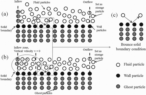
The original recycle boundary condition has disadvantages due to the fact that the velocities of the clear flow region and porous region are quite different and the newly added fluid particles usually introduce velocity fluctuations near the inflow zone. Therefore, a developed recycle boundary condition is utilized in this study to overcome this problem. As shown in Figure 1b, a stabilized inflow zone has been set up near the inflow boundary, in which the injection of storage particles is based on the distance between the first layer of ghost particles beyond the domain and the closest fluid particles in the inflow zone in which the vertical velocity is removed from these fluid particles. The injection of fluid particles is different from the original recycle boundary condition which injects fluid particles based on simulation time. If the distance is more than the particle distance D_L, one fluid particle will be added into the simulation domain. Thus, the free surface becomes more stable near the inflow boundary compared to the original recycle boundary condition in MPS method.

3.3. Interfacial condition

The interfacial condition is crucial during the simulation in this study. The interfacial condition used in numerical methods of channel flow over porous bed represents the effects from the porous flow region; some of the previous numerical studies introduced a slip velocity as the interfacial condition for simplicity, another widely used interfacial boundary condition is jump stress condition, which has also been successfully utilized in mesh-based methods (Deresiewicz & Skalak, 1963; Ochoa-Tapia & Whitaker, 1995; Pedras & de Lemos, 2001; Vollmera, Ramos, Daebel, & Kuhn, 2002). However, the interfacial condition defined in this study for the channel flow over porous bed simulation is different from these used in mesh-based methods as shown in Figure 2.

Figure 2. Interfacial boundary and velocity in MPS method.

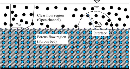
The flow velocity in clear flow region is usually much greater than the flow velocity in the porous flow region. Therefore, the value of the interfacial velocity u_int between these two regions is difficult to determine. In mesh-based methods, with the help of computational grids, the interfacial velocity can be calculated in terms of its position on the interface grid by averaging the velocities of nearby grids. Traditionally, variable grid scales are used for different flow regions in order to increase the simulation efficiency, and an additional equation near the interface is required to calculate the momentum transfer. Mesh-free particle method does not need special treatment for the momentum transfer near the interface since water particles can move freely between the clear flow region and porous flow region. However, the interfacial velocity cannot be determined easily in mesh-free particle methods. Hereafter, a background-grid-based interfacial condition will be implemented to represent the interfacial velocity and shear stress. This method is successfully implemented to simulate the interaction between a solitary wave and a submerged wave breaker (Huang et al., 2003) and is also successfully used in simulating solitary wave interaction with porous media by the SPH (Smoothed Particle Hydrodynamics) method (Shao 2010). To utilize this interfacial condition, background grids are configured at the same level of the interface, and the spatial interval of the background grids equals the particle distance D_L. The interfacial flow velocity, pressure, and shear stress are calculated on the interfacial grids by averaging the corresponding flow characteristics of the neighbor particles. Figure 2 shows the interfacial condition used in MPS method. The red dots on the interface line are the interfacial grids. The characteristics such as flow velocity and pressure are easy to calculate for interfacial grid nodes using kernel function. Basically, the interfacial velocity is calculated only at the virtual interfacial grid nodes and assigned to the particles close to the specific grid node. When assigning the interfacial velocity to the nearby fluid particles, only these particles, either in the clear flow region or porous flow region, which are close to the interface within the particle distance D_L will be involved. The interface background grid line shown in Figure 2 is a virtual grid line, which does not participate in the calculation of fluid flow during the simulation. Thus, this interfacial condition does not change the inherent characteristics of the particle method.

The interfacial velocity and stress are calculated based on the continuous interfacial condition which is given as (Huang et al., 2003; Shao, 2010): (13) (14) (15) (16) where the subscript f denotes the clear flow region and the subscript p denotes the porous flow region. The above equations show that the streamwise velocity u, the vertical velocity v, the normal stress and shear stress in the clear flow region and porous flow region are the same at the interface. The interfacial velocity is first calculated based on the clear flow velocity and porous flow velocity of those particles near the interface and assigned to the interfacial background grid, the normal stress and shear stress are then calculated for the nearby particles, the interfacial velocity u_int is then assigned to the particles inside the search area around the corresponding background grid.

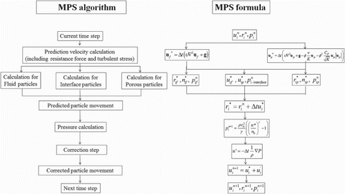
In this study, a forward differentiation is introduced for the time splitting, and a simple prediction-correction algorithm is used in a single time step, which is quite similar with the prediction-correction approach used in mesh-based method. The interfacial velocity, pressure, and shear stress calculations use the characteristics calculated from the prediction step (Press, Teukolsky, Vetterling, & Flannery, 2007), and the calculated characteristics are then utilized in the correction step. The revised MPS simulation algorithm is shown in Figure 3, in which the superscript asterisk (*) denotes the prediction parameters, the superscript apostrophe denotes the correction parameters, and the superscript ‘n’ denotes the current simulation time step.

Figure 3. Revised prediction-correction MPS algorithm.

4. Channel flow over porous bed

4.1. Testing case: laminar channel flow over porous bed

As the simplest flow pattern in channel flow over porous bed, the laminar flow over and within porous bed is applied. The Forchheimer’s term in Eq. (4) (the last term in equation 2) does not play an important role in this case study since the porous velocity is quite small, so the Darcy’s term, then, governs the porous flow in this case study.

The analytical solution of the laminar channel flow over porous bed is derived by Poulikakos and Kazmierczak (1987) and is given as:

For the clear flow region, (17)

For the porous flow region, (18) where h_f is the clear flow region depth, y is the vertical distance to the interface level, H is the total channel depth including both in the clear flow region and porous flow region, Da is the Darcy number, Da = K/H², K is the permeability, and A = (H²/μ)(ρgS₀) is the reference velocity, where S₀ is the channel bed slope.

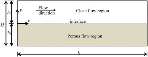
The flow conditions used in the MPS simulation are the same as the numerical case of Prinos et al. (2003). The numerical configuration is similar as shown in Figure 4. The total depth of the simulation domain H = 0.105 m, the depth of the clear flow region h_f = 0.05 m, the depth of the porous flow region h_p = 0.055 m, simulation time step dt = 0.001 s, the shear velocity U* = 2.232 × 10⁻⁴ m/s, bed slope S₀ = 1.021 × 10⁻⁷, porosity φ = 0.44, permeability K = 5.55 × 10⁻⁷ m², and ρgS₀ = 0.001 N/m³. In this study, the channel length is selected as L = 6 m. The fluid flow velocity in the clear flow region is u_f = 8.6 × 10⁻⁴ m/s. Therefore, the R_ef is kept at 42.76 to ensure laminar flow conditions during simulation, and the porous Reynolds number R_ep is kept at 0.012 to ensure the Darcy flow regime (Pedras & de Lemos, 2001). Additionally, the Froude number in this case equals 0.0019 due to u_fmax = 0.00133 m/s and h_f = 0.05 m is used.

Figure 4. Description of MPS computational domain.

Prinos et al. (2003) provided both a microscopic numerical model and analytical solution for laminar channel flow over porous bed. Their microscopic model reproduced a detailed porous medium structure using a very fine grid size of 10⁻⁵ m. However, a particle size of D_L = 0.005 m is used in the macroscopic MPS modeling. The comparison among present macroscopic MPS model, Prinos’ microscopic model, and the analytical solution is shown in Figure 5.

Figure 5. Streamwise velocity comparison of laminar flow over porous bed.

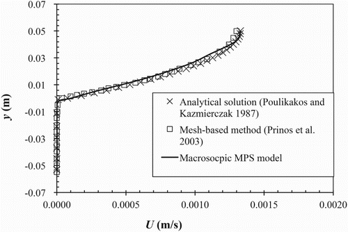
From the streamwise velocity comparison shown in Figure 5, both Prinos’ microscopic method and the present macroscopic MPS model are in very good agreement with the analytical solution. Indeed, under laminar flow conditions, the streamwise velocity is too small to show significant velocity discrepancies. The present MPS model overpredicts the interfacial velocity and surface velocity but underpredicts the velocity along the vertical section compared to the analytical solution, while the traditional mesh-based method also provides a good velocity profile near the interface and free surface. The present model shows acceptable results compared to both the numerical results from mesh-based method and the analytical solution under the same flow conditions.

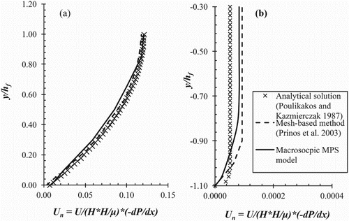
The detailed dimensionless velocity comparison shown in Figure 6 includes two flow regions. In the clear flow region, both the results obtained from the MPS model and Prinos’ numerical model are close to the analytical solution. In the porous flow region, the MPS model shows a closer result to the analytical solution compared to Prinos’ model, although both of these numerical models overestimate the porous velocity during the simulation and show some discrepancies, especially near the channel bottom. From the comparison shown in Figure 6, with the additional term introduced in governing equation, MPS method successfully simulated the laminar flow over porous bed with only minor discrepancies.

Figure 6. Detailed dimensionless velocity comparison (a) clear flow region (b) porous flow region.

4.2. Testing case: turbulent channel flow over porous bed

The second case study is to solve turbulent channel flow over porous bed. The Forchheimer’s term in Eq. (4) is important in porous flow simulation since the porous Reynolds number R_ep is kept at 218 in this case to ensure the Forchheimer flow regime (Pedras & de Lemos, 2001). Hence, the Darcy’s term is not sufficient to represent the flow pattern adequately in high porous velocity simulation, therefore, the Darcy-Forchheimer terms are both used in the momentum equation for the porous flow simulation in this case study.

In this application, the parameters such as the total depth H, clear flow depth h_f, and porous flow depth h_p and simulation time step dt are similar to those parameters in the laminar flow case. Therefore, the particle distance D_L is also the same as the laminar flow case. The porosity equals 0.83, the permeability equals 4.1 × 10⁻⁴ m², and the channel bed slope equals 2.004 × 10⁻³, which make the driven force ρgS₀ equals to 19.62 N/m³. The Reynolds number R_ef equals 1.2 × 10⁴ in this case, and the Froude number equals 0.44 in this case due to u_fmax = 0.305 m/s and h_f = 0.05 m are obtained. Prinos et al. (2003) also provided a mesh-based numerical method to simulate turbulent channel flow over porous bed on the basis of an experimental study. Therefore, comparisons are made among measured data, Prinos’ mesh-based model, and the macroscopic MPS model, as shown in Figure 7.

Figure 7. Streamwise velocity comparison of turbulent channel flow over porous bed.

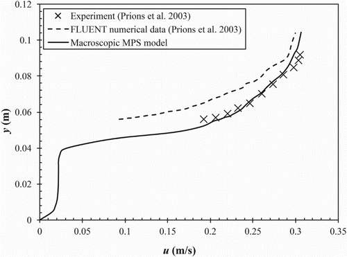
Actually, the instantaneous simulation results of MPS method depends on the particle size as indicated by previous research (Fu & Jin, 2014), using a fine particle size will give more accurate instantaneous simulation results but will lead to a much longer simulation time, and vice versa. In this study, considering both the simulation accuracy and efficiency, proper particle size is selected for each simulation case, and a 10 s time-averaging is applied to obtain MPS results.

In Figure 7, 10 s time-averaged is applied to MPS results, which still show some fluctuations since the particle’s movement is more violent compared to the laminar flow case. However, the results obtained from the MPS method are in good agreement with the measured data. The traditional mesh-based method underestimates the velocity along the whole comparison section. Both the interfacial velocity and free surface velocity obtained from the MPS model are better than those in the mesh-based method. Indeed, these two numerical methods both show discrepancies from the measured data. However, since it is more difficult to reproduce the interfacial condition than the free surface condition in numerical studies, the discrepancies are larger near the interface but smaller near the water surface in the results obtained by both numerical methods. Regretfully, the velocity measurements in the porous flow region are not available in this case study. Therefore, the comparison of porous flow velocity cannot be provided. However, the macroscopic MPS model ensures similar flow behavior under turbulent flow conditions in clear flow region, which has seldom been considered and simulated in particle methods before. Thus, this particle-based method is capable of dealing with both laminar and turbulent flow over porous bed.

4.3. Comparison of MPS and DNS of channel flow over porous media

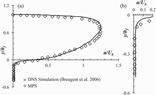
A simple simulation case is conducted first to test the newly-developed MPS method, the present simulation results are compared to previous DNS (Direct Numerical Simulation) studies by Breugem et al. (2006) as shown in Figure 4.

The channel L is 0.3 m, h_f = h_p = 0.03 m (Breugem et al., 2006), porosity of the porous bed  = 0.95, and simulation time step dt = 0.00125 s.

As shown in Figure 8, the 10 s time-averaged simulated results from MPS predict the velocity profile well in both the clear flow region and porous flow region, although some discrepancies and numerical instabilities are found in the MPS result, the MPS results are smaller than the DNS simulation below y/h_f = 0.6 and greater than DNS simulation results above y/h_f = 0.6. The simulated velocity profile shows a slightly different interfacial velocity and smaller velocity profile above y/h_f = 0.6 due to the effects from the top wall of which the MPS method introduced a simple bounce boundary condition to represent the solid top wall. In the porous flow region, the MPS method actually slightly underpredicts the porous velocity by about 20% compared to the DNS simulation data, which may be due to the fact that a macroscopic model is used for simulating the porous medium flow in this study and leads to the discrepancies in porous velocity comparison. However, the mesh-free particle-based macroscopic MPS method show close simulation results compared to previous DNS simulation and confirms its capability in predicting the channel flow over porous bed phenomenon.

Figure 8. Dimensionless mean-streamwise-velocity comparison (a) Both clear flow region and porous flow region, (b) Enlarged porous flow region.

5. Channel flow over object lying on porous bed

5.1. Channel flow over a rigid box

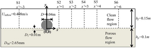
From the discussions in the previous sections, the capacity of the macroscopic MPS model in simulating channel flow over permeable bed has been confirmed. Hereafter, a two-dimensional channel flow over a rigid box placed on permeable bed is considered based on previous experimental study by Suga, Tominaga, Mori, & Kaneda (2013). Both the effects of the solid box and the permeable bed are considered in this simulation case to show the capability of the MPS method in reproducing the fluid flow of two-dimensional channel flow over an obstacle placed on a permeable bed. Although the velocity profiles in the porous medium are not available, the effects from the permeable bed are represented by the channel bed velocity which is not equal to zero compared to the impermeable bed. Additionally, several simulation cases of the channel flow over a rigid box placed on permeable bed regarding different clear flow Reynolds numbers are conducted and the simulated clear flow velocity profiles at different sections are compared with experimental data.

The numerical setup is similar to the experimental setup (Figure 9) in which h_f = h_p = 0.03 m. The channel length L = 2 m in MPS simulation which is 4 m in the experiment in order to reduce the total particle number and improve the simulation efficiency. The simulation time step dt = 0.002 s. A square rigid box with height h = 0.015 m is placed on the porous bed in the middle of the simulation domain. The porosity and permeability of the porous bed are set the same as in the experiment. Two groups of the porosity and permeability are considered in this study, which are φ = 0.82 and K = 0.02 mm² for simulation group A and φ = 0.80 and K = 0.087 mm² for simulation group B.

Figure 9. Configuration of channel flow over a rigid box on porous bed.

The comparison between experimental and time-averaged MPS results are shown in Figures 10 to 14. The origin of the simulation domain located at the right toe of the rigid box. Two typical clear Reynolds numbers, R_ef = 1000 and R_ef = 10000, have been tested in different groups. Hence, in total four sets of simulations are conducted with different porous bed characteristics and clear flow Reynolds numbers. Moreover, five comparison sections S1 to S5, located before, above and behind the rigid box, are selected to compare the mean streamwise velocity. The locations of the sections and the origin of the simulation domain are also shown in the configuration figure (Figure 9).

Figure 10. Streamwise velocity comparison. Group A, R_ef = 1000.

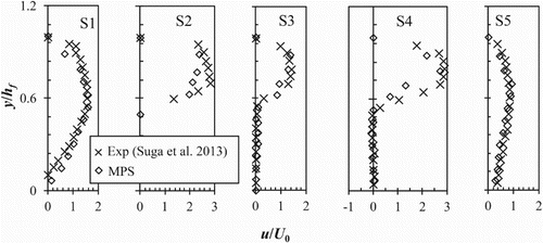
Figure 11. Streamwise velocity comparison. Group A, R_ef = 10000.

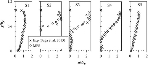
Figure 12. Streamwise velocity comparison. Group B, R_ef = 1000.

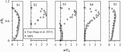
Figure 13. Streamwise velocity comparison. Group B, R_ef = 10000.

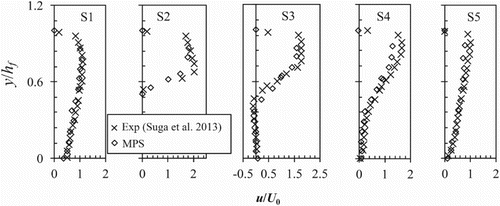
Figure 14. Configuration of open channel flow over a cylinder on porous bed.

As shown in the figures of streamwise velocity comparison, the velocity profiles in the clear flow region agree well with experimental data in all the figures for different simulation setups considering different clear flow Reynolds numbers and porous bed permeability, although discrepancies are obtained with the increasing of clear flow Reynolds number.

At S1 (x/h = −2), the simulated velocity profiles show good agreement with experimental data in all the simulation cases although minor discrepancies are obtained near the top of the simulation domain due to the fact that in MPS simulation the bounce boundary condition is applied as the solid boundary condition on the top of the channel flow. At S2 (x/h = −0.5), the velocity profile above the rigid box still shows discrepancies near the rigid box and the top wall while the velocity profile between the rigid box and the top wall show close results between MPS results and experimental data. For S3 (x/h = 0.5) and S4 (x/h = 2.0), the velocity profiles reveal the scour behind the rigid box. Due to the effects from the porous bed, the simulated velocity profiles from S3 to S4 show discrepancies especially in Group A in which the lower permeability lead to an unstable and fluctuating interface during the simulation. Thus, the MPS results show differences near the interface compare to experimental data for Group A cases. However, the scouring is clearly reproduced in MPS results due to the fact that the recovery of the velocity from S3 to S4 is obtained in the present study. Additionally, at S5 (x/h = 8.0) the velocity profiles obtained from MPS model and experiment again matched well since the location of S5 is away from the rigid box and the clear flow velocity in MPS result behaves similar to channel flow as indicated by Suga et al. (2013).

5.2. Open channel flow over a cylinder

From the discussions in the previous sections, the capacity of the macroscopic MPS model in simulating open channel flow over porous bed has been confirmed. Dey, Sarkar, Bose, Tait, and Castro-orgaz (2011) measured the wake flows behind a cylinder placed on porous bed. Their measured velocity profile shows the characteristics of flow over a cylinder on porous bed, although the water flow inside the porous bed is not investigated. Their measurements provided the velocity profiles in the clear flow region, and interfacial velocities are also available. Therefore, it is selected as an additional simulation case to test the model. The experimental configuration is shown in Figure 14.

In the experiment, the gravel size of the porous bed is given as D₅₀ = 2.65 mm. Since the porosity φ and permeability K are required in Eq. (4), it is necessary to establish a relationship between the porous gravel size D₅₀ and the porosity as well as the permeability. Wu and Wang (2006) developed an empirical equation given as: (19)

For a simple porous medium, there is an inherent relationship among the porosity φ, permeability K, and the medium gravel size D₅₀ if these values are not given by experiment. They can be calculated by the equation given as (Fumoto et al., 2012): (20)

In the present MPS simulation, the length of the domain L is 4 m and the cylinder is placed horizontally in the middle of the simulation domain. The diameter of the cylinder is D = 0.04 m, and one quarter of the cylinder, D₂ = 0.01 m, is immersed in the porous bed. The initial particle distance D_L = 0.005 m, a total of 42880 particles is assigned to the flow domain, and simulation time step dt in this case is 0.0016 s. The inflow velocity u_inflow = 0.408 m/s from the experiment is also used as the inflow velocity in the MPS simulation. The porosity φ = 0.30 and permeability K = 3.69 × 10⁻⁹ m² are estimated from Eq. (19) and Eq. (20), respectively.

The streamwise velocity of six sections are selected for comparison as shown in Figure 15, where x’ = x/D, x is the horizontal distance measured from the center of the cylinder, and D is the diameter of the cylinder.

Figure 15. Velocity comparisons between experimental data and Macroscopic MPS model.

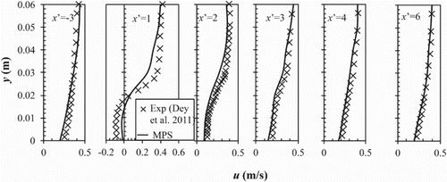
As shown in Figure 15, the velocity profile along the vertical section is close to the measured data at different comparison sections, and the interactions between clear flow and porous flow regions lead to a high interfacial velocity. In Figure 15, S1 is located upstream of the cylinder, and the velocity profile at S1 is quite similar to the open channel flow over porous bed case, which also represents the approaching velocity.

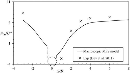
The comparison of normalized interfacial velocity (interfacial velocity u_int / shear velocity U*) near the channel bed obtained from the MPS model and measurements are shown in Figure 16 for sections S1 to S6 (x′ = −3 to x′ = 6). The interfacial velocity at S1 equals approximately 0.2 m/s, which is close to but slightly smaller than the measured data. S2 (x′ = 1) through S5 (x′ = 4) reveal the velocity variations as well as the wake flow zone behind the cylinder. At S2, wake flow velocity appears and the interfacial velocity is quite small since S2 is located right behind the cylinder. S3 (x′ = 2) to S5 are the wake zones in which the velocity profile begins to recover from S2. S6 (x′ = 6) located far from the cylinder, and the velocity profile at S6 is quite similar to S1; the MPS results, again, show good agreement with the measured data. The discrepancies give rise to the estimated porosity and permeability from Eq. (19) and Eq. (20) enhance the effects from the porous bed and reduce the interfacial velocity. However, both the MPS results and measured data show a decreasing interfacial velocity before the cylinder and an increasing interfacial velocity behind the cylinder, which also confirms the effects of the cylinder in this case. The interfacial velocity obtained by the MPS model demonstrates the strong capability of the macroscopic MPS model for representing the interface between the porous flow region and the clear flow region, which has been neglected in most of the previous studies.

Figure 16. Dimensionless interfacial velocity comparison.

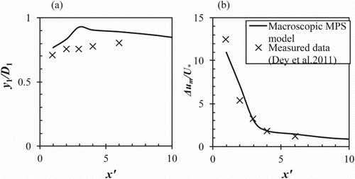
Figure 17 shows the similarity of the velocity defect at different comparison sections where D₁ is the height of the cylinder above the porous bed, Δu is the velocity defect, and Δu = U(y)-u(y) where U(y) is the approach velocity and u(y) is the streamwise velocity at vertical location y, Δu_m is the maximum velocity defect at x′, and y₁ is the vertical location where half of the maximum velocity defect occurs. The velocity defects varied rapidly among different sections because of the existence of the cylinder. Velocity defects will be larger at the sections closer to the cylinder, the results obtained from the MPS method show the same tendency as the measured data, although velocity fluctuates during the calculation. The MPS results shown in Figure 17a indicate that the location of half of the maximum velocity defect in MPS is slightly at variance with the measured data, which might be due to the fact that the approaching velocity and the velocity profile in the MPS results both slightly differ from the measured data. Figure 17b shows that the calculated Δu_m/U* in different sections of x′ are similar to the measured data. It also reveals the similarity of the flow behavior in the wake zone behind the cylinder between the numerical results and measured data from x′ = 0 to x′ = 10.

Figure 17. Dimensionless comparison (a) location of velocity defect, (b) variations of peak velocity defect.

6. Conclusion

In this study, a macroscopic MPS model is developed to investigate channel flow over porous bed. With this Lagrangian approach, the flow behavior near the free surface is easy to obtain in the current MPS model, the simulation of flow behavior between clear flow and porous flow regions is given more attention in this study. Both Darcy’s and Forchheimer’s terms are introduced in the simulation for channel flow over porous bed. A modified inflow boundary condition and an interfacial condition are successfully implemented. The particle-based method has then been extended to the porous medium flow simulation. The comparisons among experimental data, analytical solution, numerical results from traditional mesh-based method, and the present model show that the macroscopic MPS method is good at simulating both the clear flow region and porous flow region. Additionally, channel flow over a rigid box on porous bed case is simulated. Various comparisons of velocity profiles between MPS results and measured data at different sections indicate that the present MPS model predicts well in the interfacial velocity and the wake zone behind the rigid box while the effects from interfacial velocity near the channel bed are also represented well in the new macroscopic MPS model.

With all the simulations and comparisons, the developed macroscopic MPS method has proven a reasonable tool in porous medium flow simulation. This macroscopic MPS model is valuable in the areas of beach erosion and inundation or mud flow simulation, in which both the free surface and porous medium flow play important roles. Moreover, this developed macroscopic MPS method can be used to study variable porosity and permeability in porous media. Microscopic porous flow simulation, multiphase flow simulation, and interfacial flow simulation will also be possible by using the particle methods on the basis of the development of more efficient macroscopic MPS model in the future.

Notations

CF	=	Forchheimer’s coefficient
d	=	Number of space dimensions
dc	=	Characteristic length (m)
DL	=	Initial Particle distance in MPS method (m)
Da	=	Darcy’s number = K/H2
D50	=	Medium diameter of gravel (m)
f	=	Body force
Frf	=	Clear flow region Froude number
g	=	Gravitational acceleration (ms−2)
H	=	Water depth (m)
hf	=	Clear flow depth (m)
hp	=	Porous flow depth (m)
K	=	Permeability (m2)
ks	=	Roughness height (m)
i	=	Specific target particle
j	=	Neighbor particle
L	=	Length of the channel (m)
n0	=	Initial particle number density (-)
n*	=	Calculated particle number density (-)
r	=	Particle position vector (m)
Ra	=	Particle searching radius (m)
Ref	=	Clear flow region Reynolds number
Rep	=	Porous flow region Reynolds number
S0	=	Channel bed slope
t	=	Time (s)
U*	=	Shear velocity (ms−1)
Un	=	Dimensionless streamwise velocity component
u	=	Components of velocity vector in x direction (ms−1)
u	=	Velocity vector (ms−1)
uinflow	=	Inflow velocity (ms−1)
uint	=	Interfacial velocity (ms−1)
uf	=	Clear flow region velocity (ms−1)
ufmax	=	Maximum clear flow region velocity (ms−1)
up	=	Porous flow velocity (ms−1)
x, y	=	Cartesian components (m)
x′	=	Dimensionless Cartesian components
ρ	=	Fluid density (kgm−3)
μ	=	Dynamic viscosity (kgm−1s−1)
ν	=	Kinematic viscosity (m2s−1)
φ	=	Porosity
Ψ	=	General factor or scalar

Disclosure Statement

No potential conflict of interest was reported by the authors.

Additional information

Funding

This research was supported in part by the Natural Sciences and Engineering Research Council of Canada (109585-2012).

References

- Alazmi, B., & Vafai, K. (2001). Analysis of fluid flow and heat transfer interfacial conditions between a porous medium and a fluid layer. International Journal of Heat and Mass Transfer, 44, 1735–1749. doi: 10.1016/S0017-9310(00)00217-9
- Beavers, G. S., & Joseph, D. D. (1967). Boundary conditions at a naturally permeable wall. Journal of Fluid Mechanics, 30, 197–207. doi: 10.1017/S0022112067001375
- Breugem, W. P., Boersma, B. J., & Uittenbogaard, R. E. (2006). The influence of wall permeability on turbulent channel flow. Journal of Fluid Mechanics, 562, 35–72. doi: 10.1017/S0022112006000887
- Chan, H. C., Huang, W. C., Leu, J. M., & Lai, C. J. (2007). Macroscopic modeling of turbulent flow over a porous medium. International Journal of Heat and Fluid Flow, 28, 1157–1166. doi: 10.1016/j.ijheatfluidflow.2006.10.005
- Chen, X., & Chiew, Y. (2004). Velocity distribution of turbulent open-channel flow with bed suction. Journal of Hydraulic Engineering, 130, 140–148. doi: 10.1061/(ASCE)0733-9429(2004)130:2(140)
- Colagrossi, A., & Landrini, M. (2003). Numerical simulation of interfacial flows by smoothed particle hydrodynamics. Journal of Computational Physics, 191(2), 448–475. doi: 10.1016/S0021-9991(03)00324-3
- Delft3D WL|delft hydraulics. (2001). User manual Delft3D-FLOW, Delft3D-WAQ and Delft3D-PART. Delft: WL|delft hydraulics.
- Deresiewicz, H., & Skalak, R. (1963). On uniqueness in dynamic poroelasticity. Bulletin of the Seismological Society of America, 53, 783–788.
- Dey, S., Sarkar, S., Bose, S. K., Tait, S., & Castro-orgaz, O. (2011). Wall-Wake flows downstream of a sphere placed on a plane rough wall. Journal of Hydraulic Engineering, 137(10), 2005–2010. doi: 10.1061/(ASCE)HY.1943-7900.0000441
- Federico, I. (2010). Simulating open-channel flows and advective diffusion phenomena through SPH model ( Phd thesis). Università della Calabria.
- Fluent Inc. (1998). Fluent user’s guide, version 5.0. New Hampshire: Fluent Inc.
- Fu, L., & Jin, Y.-C. (2013). A mesh-free method boundary condition technique in open channel flow simulation. Journal of Hydraulic Research, 51(2), 174–185. doi: 10.1080/00221686.2012.745455
- Fu, L., & Jin, Y.-C. (2014). Simulating velocity distribution of dam breaks with the particle method. Journal of Hydraulic Engineering, 140(10), 1–10. doi: 10.1061/(ASCE)HY.1943-7900.0000915
- Fumoto, Y., Liu, R., Sano, Y., & Huang, X. (2012). A three-dimensional numerical model for determining the pressure drops in porous media consisting of obstacles of different sizes. The Open Transport Phenomena Journal, 4, 1–8. doi: 10.2174/1877729501204010001
- Gotoh, H., Shibahara, T., & Sakai, T. (2001). Sub-particle-scale turbulence model for the MPS method—Lagrangian flow model for hydraulic engineering. Computational Fluid Dynamics Journal, 9(4), 339–347.
- Gui, Q., Dong, P., Shao, S., & Chen, Y. (2015). Incompressible SPH simulation of wave interaction with porous structure. Ocean Engineering, 110(A), 126–139. doi: 10.1016/j.oceaneng.2015.10.013
- Harlow, F. H., & Welch, J. E. (1965). Numerical calculation of time-dependent viscous incompressible flow of fluid with free surface. Physics of Fluids, 8, 2182–2189. doi: 10.1063/1.1761178
- Hirt, C. W., & Nichols, B. D. (1981). Volume of fluid (VOF) method for the dynamics of free boundaries. Journal of Computational Physics, 39(1), 201–225. doi: 10.1016/0021-9991(81)90145-5
- Huang, C.-J., Chang, H.-H., & Hwung, H.-H. (2003). Structural permeability effects on the interaction of a solitary wave and a submerged breakwater. Coastal Engineering, 49, 1–24. doi: 10.1016/S0378-3839(03)00034-6
- Jambhekar, V. A. (2011). Forchheimer porous-media flow models – numerical investigation and comparison with experimental data (Master’s thesis). Universität Stuttgart.
- Jiang, F., Oliveira, M. S. A., & Sousa, A. C. M. (2007). Mesoscale SPH modeling of fluid flow in isotropic porous media. Computer Physics Communications, 176(7), 471–480. doi: 10.1016/j.cpc.2006.12.003
- Kondo, M., & Koshizuka, S. (2011). Improvement of stability in moving particle semi-implicit method. International Journal for Numerical Methods in Fluids, 65(6), 638–654. doi: 10.1002/fld.2207
- Koshizuka, S., & Oka, Y. (1996). Moving-particle semi-implicit method for fragmentation of incompressible fluid. Nuclear Science and Engineering, 123, 421–434.
- Koshizuka, S., Tamako, H., & Oka, Y. (1995). A particle method for incompressible viscous flow with fluid fragmentation. Computational Fluid Dynamics Journal, 4, 29–46.
- Kunz, P., Zarikos, I. M., Karadimitriou, N. K., Huber, M., Nieken, U., & Hassanizadeh, S. M., (2016). Study of multi-phase flow in porous media: Comparison of SPH simulations with micro-model experiments. Transport in Porous Media, 114(2), 581–600. doi: 10.1007/s11242-015-0599-1
- Lage, J. L. (1998). The fundamental theory of flow through permeable media: From Darcy to turbulence. In D. B. Ingham and I. Pop (Eds.), Transport phenomena in porous media (pp. 1–30). Oxford, UK: Elsevier Science.
- Leu, J. M., Chan, H. C., Tu, L.-F., Jia, Y., & Wang, S. Y. (2009). Velocity distribution of non-darcy flow in a porous medium. Journal of Mechanics, 25(1), 49–58. doi: 10.1017/S1727719100003592
- Li, B. (1990). Characteristics of flow in rough channels with permeable bed. Proceedings of 7th congress APD-IAHR, Chinese Association for Hydraulic Research, Beijing, 1–7.
- Liu, G. R., & Liu, M. B. (2003). Smoothed particle hydrodynamics a Meshfree particle method. New Jersey, USA: World Scientific Publishing Company.
- Manes, C., Pokrajac, D., McEwan, I., & Nikora, V. (2009). Turbulence structure of open channel flows over permeable and impermeable beds: A comparative study. Physics of Fluids, 21, 207. doi: 10.1063/1.3276292
- Miglio, E., Quarteroni, A., & Saleri, F. (2003). Coupling of free surface and groundwater flows. Computers & Fluids, 32, 73–83. doi: 10.1016/S0045-7930(01)00102-5
- Monaghan, J. J., & Gingold, R. A. (1983). Shock simulation by the particle method SPH. Journal of Computational Physics, 52, 374–389. doi: 10.1016/0021-9991(83)90036-0
- Nakamura, Y., & Stefan, H. G. (1994). Effect of flow velocity on sediment oxygen demand: Theory. Journal of Hydraulic Engineering, 120(5), 996–1016.
- Nazari, F., Jin, Y.-C., & Shakibaeinia, A. (2012). Numerical analysis of jet and submerged hydraulic jump using moving particle semi-implicit method. Canadian Journal of Civil Engineering, 39(5), 495–505. doi: 10.1139/l2012-023
- Neale, G., & Nader, W. (1974). Practical significance of Brinkman’s extension of Darcy’s law: Coupled parallel flows within a channel and a bounding porous medium. The Canadian Journal of Chemical Engineering, 52, 475–478. doi: 10.1002/cjce.5450520407
- Nikora, V. I., Goring, D. G., McEwan, I., & Griffiths, G. (2001). Spatially averaged open-channel flow over rough Bed. Journal of Hydraulic Engineering, 127(2), 123–133. doi: 10.1061/(ASCE)0733-9429(2001)127:2(123)
- Nikora, V. I., McEwan, I., McLean, S., Coleman, S., Pokrajac, D., & Walters, R. (2007). Double-averaging concept for rough-bed open-channel and overland flows: Theoretical back-ground. Journal of Hydraulic Engineering, 133(8), 873–883. doi: 10.1061/(ASCE)0733-9429(2007)133:8(873)
- Ochoa-Tapia, J. A., & Whitaker, S. (1995). Momentum transfer at the boundary between a porous medium and a homogeneous fluid—I. Theoretical development. International Journal of Heat and Mass Transfer, 38, 2635–2646. doi: 10.1016/0017-9310(94)00346-W
- Pahar, G., & Dhar, A. (2016). Modeling free-surface flow in porous media with modified incompressible SPH. Engineering Analysis with Boundary Elements, 68, 75–85. doi: 10.1016/j.enganabound.2016.04.001
- Pedras, M. H. J., & de Lemos, M. J. S. (2001). Macroscopic turbulence modeling for incompressible flow through undeformable porous media. International Journal of Heat and Mass Transfer, 44(6), 1081–1093. doi: 10.1016/S0017-9310(00)00202-7
- Pokrajac, D., & Manes, C. (2009) Velocity measurements of a free-surface turbulent flow penetrating a porous medium composed of uniform-size spheres, Transport in Porous Media, 78(3), 367–383. doi: 10.1007/s11242-009-9339-8
- Pokrajac, D., Manes, C., & McEwan, I. (2007). Peculiar mean velocity profiles within a porous bed of an open channel. Physics of Fluids, 19, 098–109. doi: 10.1063/1.2780193
- Poulikakos, D., & Kazmierczak, M. (1987). Forced convection in a duct partially filled with a porous material. Journal of Heat Transfer, 109, 653–662. doi: 10.1115/1.3248138
- Press, W. H., Teukolsky, S. A., Vetterling, W. T., & Flannery, B. P. (2007). Section 17.6. Multistep, multivalue, and predictor-corrector methods. Numerical recipes: The art of scientific computing (3rd ed.). New York: Cambridge University Press. ISBN 978-0-521-88068-8.
- Prinos, P., Sofialidis, D., & Keramaris, E. (2003). Turbulent flow over and within a porous Bed. Journal of Hydraulic Engineering, 129(9), 720–733. doi: 10.1061/(ASCE)0733-9429(2003)129:9(720)
- Rudraiah, N. (1985). Coupled parallel flows in a channel and a bounding porous medium of finite thickness. Journal of Fluids Engineering, 107, 322–329. doi: 10.1115/1.3242486
- Sahraoui, M., & Kaviany, M. (1992). Slip and no-slip velocity bound-ary conditions at interface of porous, plain media. International Journal of Heat and Mass Transfer, 35, 927–943. doi: 10.1016/0017-9310(92)90258-T
- Shakibaeinia, A, & Jin, Y. C. (2010). A weakly compressible MPS method for modeling of open-boundary free-surface flow. International Journal for Numerical Methods in Fluids, 63, 1208–1232.
- Shao, S. (2010). Incompressible SPH flow model for wave interactions with porous media. Coastal Engineering, 57(3), 304–316. doi: 10.1016/j.coastaleng.2009.10.012
- Silva, R. A., & de Lemos, M. J. S. (2003). Numerical analysis of the stress jump interface condition for laminar flow over a porous layer. Numerical Heat Transfer, Part A: Applications, 43(6), 603–617. doi: 10.1080/10407780307351
- Souto-Iglesias, A., Macià, F., González, L. M., & Cercos-Pita, J. L. (2013). On the consistency of MPS. Computer Physics Communications, 184(3), 732–745. doi: 10.1016/j.cpc.2012.11.009
- Steinberger, N., & Hondzo, M. (1999). Diffusional mass transfer at sediment-water interface. Journal of Environmental Engineering, 125(2), 192–200. doi: 10.1061/(ASCE)0733-9372(1999)125:2(192)
- Suga, K., Tominaga, S., Mori, M., & Kaneda, M. (2013). Turbulence characteristics in flows over solid and porous square ribs mounted on porous walls. Flow, Turbulence and Combustion, 91(1), 19–40. doi: 10.1007/s10494-013-9452-1
- Svensson, U., & Rahm, L. (1991). Toward a mathematical model of oxygen transfer to and within bottom sediments. Journal of Geophysical Research: Oceans, 96, 2777–2783. doi: 10.1029/90JC02209
- Trussell, R. R., & Chang, M. (1999). Review of flow through porous media as applied to head loss in water filters. Journal of Environmental Engineering, 125(11), 998–1006. doi: 10.1061/(ASCE)0733-9372(1999)125:11(998)
- Vollmera, S., Ramos, F. S., Daebel, H., & Kuhn, G. (2002). Micro scale exchange processes between surface and subsurface water. Journal of Hydrology, 269, 3–10. doi: 10.1016/S0022-1694(02)00190-7
- Whitaker, S. (1986). Flow in porous media I: A theoretical derivation of Darcy’s law. Dordrecht, Holland: D. Riedel publishing company.
- Wu, W., & Wang, S. S. Y. (2006). Formulas for sediment porosity and settling velocity. Journal of Hydraulic Engineering, 132(8), 858–862. doi: 10.1061/(ASCE)0733-9429(2006)132:8(858)
- Yen, B. C. (1991). Hydraulic resistance in channels: Channel flow resistance: Centennial of manning’s formula. Littleton, CO: Water Resources Publications, 1–135.
- Zarrati, A. R., Tamai, N., & Jin, Y. C. (2005). Mathematical modeling of meandering channels with a generalized depth averaged model. Journal of Hydraulic Engineering, 131(6), 467–475. doi: 10.1061/(ASCE)0733-9429(2005)131:6(467)
- Zeng, Z., & Grigg, R. (2006). A criterion for non-Darcy flow in porous media. Transport in Porous Media, 63(1), 57–69. doi: 10.1007/s11242-005-2720-3
- Zippe, H. J., & Graf, W. H. (1983). Turbulent boundary-layer flow over permeable and non-permeable rough surfaces. Journal of Hydraulic Research, 21, 51–65. doi: 10.1080/00221688309499450